


1. Introduction
Surfactants are ‘surface-active’ molecules and/or particles that are easily adsorbed at surfaces and form monolayers (Langevin Reference Langevin2014; Manikantan & Squires Reference Manikantan and Squires2020). They are present in most multiphase systems, being either present naturally or else introduced purposefully (Levich Reference Levich1962; Stone Reference Stone1994; Soligo, Roccon & Soldati Reference Soligo, Roccon and Soldati2019; Lohse Reference Lohse2022). In bubbly flows, it has been shown that even small amounts of surfactant can cause dramatic changes to the bubble shapes (Tomiyama et al. Reference Tomiyama, Celata, Hosokawa and Yoshida2002; Tagawa, Takagi & Matsumoto Reference Tagawa, Takagi and Matsumoto2014; Hessenkemper et al. Reference Hessenkemper, Ziegenhein, Lucas and Tomiyama2021a), bubble rise velocities (Bel Fdhila & Duineveld Reference Bel Fdhila and Duineveld1996; Cuenot, Magnaudet & Spennato Reference Cuenot, Magnaudet and Spennato1997; Takagi, Ogasawara & Matsumoto Reference Takagi, Ogasawara and Matsumoto2008; Tagawa et al. Reference Tagawa, Takagi and Matsumoto2014), lateral migration (Lu, Muradoglu & Tryggvason Reference Lu, Muradoglu and Tryggvason2017; Hayashi & Tomiyama Reference Hayashi and Tomiyama2018; Ahmed et al. Reference Ahmed, Izbassarov, Lu, Tryggvason, Muradoglu and Tammisola2020; Atasi et al. Reference Atasi, Ravisankar, Legendre and Zenit2023), cluster formation (Takagi et al. Reference Takagi, Ogasawara, Fukuta and Matsumoto2009; Maeda et al. Reference Maeda, Date, Sugiyama, Takagi and Matsumoto2021; Ma et al. Reference Ma, Hessenkemper, Lucas and Bragg2023), coalescence (Verschoof et al. Reference Verschoof, Van Der Veen, Sun and Lohse2016; Lohse Reference Lohse2018; Néel & Deike Reference Néel and Deike2021) and mass transfer on the interfaces (Cuenot et al. Reference Cuenot, Magnaudet and Spennato1997; Schlüter et al. Reference Schlüter, Herres-Pawlis, Nieken, Tuttlies and Bothe2021). Some of the aforementioned effects can also occur due to the presence of salt in the liquid phase (Craig, Ninham & Pashley Reference Craig, Ninham and Pashley1993; Gvozdić et al. Reference Gvozdić, Dung, Van Gils, Bruggert, Alméras, Sun, Lohse and Huisman2019; Hori et al. Reference Hori, Bothe, Hayashi, Hosokawa and Tomiyama2020; Blaauw, Lohse & Huisman Reference Blaauw, Lohse and Huisman2023), However, the mechanisms producing these effects are different in that case.
The mechanism by which surfactants influence the velocity field in the vicinity of a gas–liquid interface was first introduced by Frumkin & Levich (Reference Frumkin and Levich1947) and Levich (Reference Levich1962), who showed that as a bubble rises in an aqueous surfactant solution, surfactant is swept off the front part of the bubble by surface convection, and accumulates in the rear region. They lower the surface tension in the rear region relative to that at the front, leading to a gradient of surface tension along the interface. This gradient creates a tangential shear stress on the bubble surface (Marangoni effect) that opposes the surface flow, causes the interface to become more rigid, and increases the drag coefficient  $C_D$. The free-slip boundary condition that occurs at a gas–liquid interface for an ideal purified system (e.g. ‘hyper-clean’ water) breaks down, and the rise speed of the contaminated bubble decreases with increasing surfactant concentration, approaching the behaviour of a rigid body for sufficient surfactant concentration.
The effect of drag coefficient increase due to the adsorption of surfactants has been studied in great detail. Readers are referred to Magnaudet & Eames (Reference Magnaudet and Eames2000), Palaparthi, Papageorgiou & Maldarelli (Reference Palaparthi, Papageorgiou and Maldarelli2006) and Takagi & Matsumoto (Reference Takagi and Matsumoto2011) for detailed reviews from the perspective of hydrodynamics, and Manikantan & Squires (Reference Manikantan and Squires2020) from the perspective of surfactant dynamics. An early study (Bachhuber & Sanford Reference Bachhuber and Sanford1974) measured the terminal velocity of small bubbles (bubble Reynolds number  $Re_p\sim O(10)$) rising in distilled water at two heights in the flow, and observed that the velocity at the lower height was in good agreement with that expected for a clean spherical bubble, while that measured at the greater height was consistent with a particle having a value of $C_D$ that corresponds to a rigid sphere. Their interesting observation reflects at least two well-known aspects of how surfactants impact bubble motion. First, water used in typical lab conditions is contaminated, possibly containing considerable amounts of surfactants that can influence the motion of bubbles. Second, it takes a finite time (which depends on the properties of the surfactants) for the surfactants to be adsorbed at the bubble surface before reaching an equilibrium state, with the implication that bubble rise velocities decrease with increasing travel distance until reaching a constant value (Durst et al. Reference Durst, Schönung, Selanger and Winter1986; Tagawa et al. Reference Tagawa, Takagi and Matsumoto2014; Hessenkemper et al. Reference Hessenkemper, Ziegenhein, Lucas and Tomiyama2021a).
The fact that the bubble rise velocity decreases in the presence of surfactants also leads to a smaller inertial force experienced by bubbles. As a result of this, for a fixed bubble size, the bubble shape is less flattened in a contaminated system than it is in a purified system, despite the fact that surface tension is reduced by surfactants.
The aforementioned modifications in bubble rise velocity, surface boundary condition and shape due to surfactants have a strong impact on the wake structure and the path instability of a rising bubble. Tagawa et al. (Reference Tagawa, Takagi and Matsumoto2014) used experiments to investigate the effect of surfactants on the path instability of an air bubble rising in quiescent water, and categorized the rising bubble trajectories as straight, helical or zigzag based on the bubble Reynolds number and surface slip condition. They observed that the trajectory of the bubble was first helical and then transitioned to a zigzag motion in Triton X-100 solution – a phenomenon never reported in purified water (Mougin & Magnaudet Reference Mougin and Magnaudet2002; Shew & Pinton Reference Shew and Pinton2006). Pesci et al. (Reference Pesci, Weiner, Marschall and Bothe2018) used numerical simulations to study the effects of soluble surfactants on the dynamics of a single spheroidal bubble rising in a large spherical domain. They found that if the surface contamination is sufficiently high, then a quasi-steady bubble velocity can be obtained over a wide range of surfactant concentrations, independent of the exact concentration value in the bulk. Furthermore, they also observed a transition from a helical to a zigzag rising bubble trajectory, as reported experimentally by Tagawa et al. (Reference Tagawa, Takagi and Matsumoto2014), but also found that the nature of the trajectory depends on both the initial surface and bulk surfactant contamination. Pesci et al. (Reference Pesci, Weiner, Marschall and Bothe2018) also looked at the vorticity dynamics in the vicinity of the bubble, and observed strong vorticity production very close to the bubble surface due to Marangoni forces, while in clean water this production is much weaker (see the vorticity distribution in figure 8 of Mougin & Magnaudet Reference Mougin and Magnaudet2006). Legendre, Lauga & Magnaudet (Reference Legendre, Lauga and Magnaudet2009) performed numerical simulations to study the two-dimensional flow past a cylinder, and investigated the influence of a generic slip boundary condition on the wake dynamics. They showed that slip markedly decreases the vorticity intensity in the wake. Mclaughlin (Reference Mclaughlin1996) and Cuenot et al. (Reference Cuenot, Magnaudet and Spennato1997) used a stagnant-cap approximation to compare the wake structure produced by contaminated bubbles and solid spheres. The former study revealed that the wake volume for contaminated bubbles is larger than for solid spheres moving at the same Reynolds number, and the latter study found that the wake length is larger for contaminated bubbles. They explained that the increase of the wake size is caused by the abrupt change to the dynamic boundary condition where the transition from a quasi-shear-free (the upper part of the bubble) to a quasi-no-slip (the rear region) condition generates strong vorticity at the interface. As a result, there is more vorticity injected into the flow for contaminated bubbles than for a rigid sphere with a uniform no-slip condition, resulting in a larger wake.
The observations summarized above were mainly for isolated bubbles in the absence of turbulence. Swarms of bubbles can, however, induce strong background turbulence, and the observations above could indicate that turbulence generated by wakes in bubble swarms could depend strongly on the degree of contamination in the fluid. Direct numerical simulations (DNS) have revealed the following properties of dilute dispersed bubbly flows. (i) The liquid velocity fluctuations are highly anisotropic, with fluctuations that are much larger in the direction of the mean bubble motion (Lu & Tryggvason Reference Lu and Tryggvason2013; Ma et al. Reference Ma, Lucas, Jakirlić and Fröhlich2020b; Ma, Lucas & Bragg Reference Ma, Lucas and Bragg2020a; du Cluzeau et al. Reference du Cluzeau, Bois, Leoni and Toutant2022; Liao & Ma Reference Liao and Ma2022). It was demonstrated recently that this strong anisotropy also exists at the small scales of bubble-induced turbulence (BIT) due to the energy being injected at the scale of the bubble (Ma et al. Reference Ma, Ott, Fröhlich and Bragg2021). (ii) The probability density functions (PDFs) of all fluctuating velocity components are non-Gaussian, with the PDF of the vertical velocity fluctuations being strongly positively skewed, while the other two directions have symmetric PDFs (Roghair et al. Reference Roghair, Mercado, Van Sint Annaland, Kuipers, Sun and Lohse2011; Riboux, Legendre & Risso Reference Riboux, Legendre and Risso2013). (iii) There is strong enhancement of the turbulent kinetic energy dissipation rate in the vicinity of the bubble surface (Santarelli, Roussel & Fröhlich Reference Santarelli, Roussel and Fröhlich2016; du Cluzeau, Bois & Toutant Reference du Cluzeau, Bois and Toutant2019). (iv) The energy spectra in either the frequency or wavenumber space exhibit a  $-3$ power-law scaling for a subrange for all the components of the fluctuating fluid velocity (Ma et al. Reference Ma, Santarelli, Ziegenhein, Lucas and Fröhlich2017; Pandey, Ramadugu & Perlekar Reference Pandey, Ramadugu and Perlekar2020; Innocenti et al. Reference Innocenti, Jaccod, Popinet and Chibbaro2021). (v) Pandey et al. (Reference Pandey, Ramadugu and Perlekar2020) and Innocenti et al. (Reference Innocenti, Jaccod, Popinet and Chibbaro2021) showed that on average, the energy transfer is from large to small scales in BIT; however, there is also evidence of an upscale transfer when considering the transfer of energy associated with particular components of the velocity field (Ma et al. Reference Ma, Ott, Fröhlich and Bragg2021). (vi) For a bubbly flow with background turbulence, the flow intermittency is increased significantly by the addition of bubbles to the flow when compared to the corresponding unladen turbulent flow with similar bulk Reynolds number (Biferale et al. Reference Biferale, Perlekar, Sbragaglia and Toschi2012; Ma et al. Reference Ma, Ott, Fröhlich and Bragg2021). Note that some of these DNS studies effectively considered contaminated bubbly flows since they used no-slip conditions on rigid bubble surfaces, while others used slip boundary conditions, and a clear understanding of exactly how the aforementioned properties of BIT depend on contaminants in the flow is not available. For further details on the relevant DNS studies, readers are referred to the recent reviews of Risso (Reference Risso2018) and Mathai, Lohse & Sun (Reference Mathai, Lohse and Sun2020).
Several experiments have also observed these properties for bubbly turbulent flows (Lance & Bataille Reference Lance and Bataille1991; Rensen, Luther & Lohse Reference Rensen, Luther and Lohse2005; Riboux, Risso & Legendre Reference Riboux, Risso and Legendre2010; Mendez-Diaz et al. Reference Mendez-Diaz, Serrano-García, Zenit and Hernández-Cordero2013; Lai & Socolofsky Reference Lai and Socolofsky2019; Salibindla et al. Reference Salibindla, Masuk, Tan and Ni2020; Masuk, Salibindla & Ni Reference Masuk, Salibindla and Ni2021; Qi et al. Reference Qi, Tan, Corbitt, Urbanik, Salibindla and Ni2022). However, in most of these experiments there will be some contamination in the liquid, and the impact of this on the results is not understood. Indeed, a systematic investigation into how contamination affects the properties of BIT is still missing, to the best of the authors’ knowledge. Therefore, in the present paper we explore systematically the effect of surfactants on the properties of BIT produced by bubble swarms, considering both single-point and two-point turbulence statistics to characterize large- and small-scale flow properties. The rest of this paper is organized as follows. In § 2, we describe the experimental set-up and the measurement techniques. We then give a brief overview regarding the effect of the surfactant on the single-bubble behaviour in the chosen solution (§ 3), followed by a presentation of the single-point statistics for the bubble swarm in § 4. Finally, the multipoint results from the experiments that give insights into the properties of the flow at different scales are divided into two parts, namely, the flow anisotropy in § 5.1, and the extreme events in § 5.2.
2. Experimental method
2.1. Experimental facility
The experimental apparatus is identical to that in Ma et al. (Reference Ma, Hessenkemper, Lucas and Bragg2022), and we therefore refer the reader to that paper for additional details; here, we summarize. Figure 1 shows a sketch of the experimental set-up, consisting of a rectangular column (depth  $50\,\mathrm {mm}$ and width $112.5\,\mathrm {mm}$) made of acrylic glass with water fill height $1100\,\mathrm {mm}$. Air bubbles are injected through $11$ spargers that are distributed homogeneously at the bottom of the column.

Figure 1. Sketch of the bubble column used in the experiments. (Note that in the actual experiment, the number of bubbles in the column is  $O(10^3)$.) The sketch is not to scale; the column depth is many times larger than the bubble diameter. The inset shows an instantaneous realization of velocity vectors over the field of view in the case LaTap (see table 1), with two in-focus bubbles recognizable by their sharp interfaces and associated wakes.
We use tap water in the present work as the base liquid, and add 1-Pentanol as an additional surfactant with varying bulk concentration  $C_\infty$ of 0, 333 and 1000 ppm. The surfactant properties and the single-bubble behaviour in these solutions will be discussed in detail in § 3.2. Note that the tap water will already be sightly contaminated prior to adding the surfactants, and the bubbles can behave differently in this tap water without surfactants compared to that in a pure water system (no surfactants; see e.g. Veldhuis, Biesheuvel & Van Wijngaarden Reference Veldhuis, Biesheuvel and Van Wijngaarden2008; Takagi & Matsumoto Reference Takagi and Matsumoto2011). For the bubble sizes considered in the present study (with $d_p>2$ mm), however, the slight contamination in the tap water does not have a significant effect on the bubble motion (Ellingsen & Risso Reference Ellingsen and Risso2001). This point was also confirmed by our previous study (Hessenkemper et al. Reference Hessenkemper, Ziegenhein, Rzehak, Lucas and Tomiyama2021b) for the bubble sizes considered here, with both the bubble rise velocity and bubble aspect ratio showing little difference between tap water and purified water systems.
We consider two different bubble sizes by using spargers with different inner diameters. For each bubble size, we maintain the same gas inlet velocity and ensure that all cases are not in the heterogeneous regime of dispersed bubbly flows. In total, we have six monodispersed cases labelled SmTap, SmPen, SmPen+, LaTap, LaPen and LaPen+ in table 1, including some basic characteristic dimensionless numbers for the bubbles. We note that the Weber number based on the liquid mean fluctuating velocity is almost two orders of magnitude smaller than the Eötvös number, indicating that the bubble deformability in the present six cases is due mainly to buoyancy rather than turbulence. Further evidence for this is provided by noting that the bubble shapes are similar to those for the single-bubble cases in § 3.2, for which the liquid turbulence is much weaker. Here, Sm/La stand for smaller/larger bubbles, and Tap/Pen/Pen+ stand for corresponding cases having 1-Pentanol concentration with  $C_\infty =0$, 333 and 1000 ppm, respectively. It should be noted that the three cases with larger bubble sizes have higher gas void fraction than the three cases with smaller bubbles. This is because in our set-up it is not possible to have the same flow rate for two different spargers while also maintaining a homogeneous gas distribution for monodispersed bubbles.
2.2. Flow imaging
2.2.1. Liquid phase
For all measurements stated below, we use a  $2.5$ megapixel CMOS camera (Imaging Solutions) equipped with a 100 mm focal length macro lens (Samyang). To measure the liquid velocity, we use particle shadow velocimetry (PSV), which is similar to planar particle image velocimetry (PIV) with the only difference being that backlight illumination together with a shallow depth of field (DoF) is used. The velocity is then determined by correlating the displacement of sharp tracer particles inside a narrow sharpness region. A detailed description of the image processing procedure used can be found in Hessenkemper & Ziegenhein (Reference Hessenkemper and Ziegenhein2018). The measurement set-up and data acquisition are similar to those in our previous work (Ma et al. Reference Ma, Hessenkemper, Lucas and Bragg2022), so only the key aspects for the liquid velocity measurements are stated in what follows.
Table 1. Selected characteristics of the six bubble swarm cases investigated. Here,  $C_\infty$ is the bulk concentration of 1-Pentanol, $\alpha$ is the averaged gas void fraction, $d_p$ is the equivalent bubble diameter, $\chi$ is the aspect ratio, $Ga\equiv \sqrt {|{\rm \pi} _\rho -1|\,gd_{p}^{3}}/\nu$ is the Galileo number, $Eo\equiv \Delta \rho \,gd_p^2/\sigma$ is the Eötvös number, $We\equiv \rho d_p{u^\ast }^2/\sigma$ is the Weber number, and $u^\ast$ is the mean fluctuating velocity. The values of $Re_p$, the bubble Reynolds number, and $C_D$, the drag coefficient, are based on $d_p$ and the slip velocity $U_r$ obtained from the experiment.

The liquid velocity measurements take place along the  $x_1$– $x_2$ symmetry plane in the centre of the depth ( $x_3$). The measurement height with $x_1 = 0.65$ m is based on the centre of the field of view (FOV) (figure 1). We use $10\,\mathrm {\mu }{\rm m}$ hollow glass spheres (Dantec) as tracer particles, with estimated Stokes number $O(10^{-3})$; they are hydrophilic and so are not adsorbed by the bubble surface. The flow section is illuminated with a 200 W LED lamp and f-stop $2.8$ is set at the camera lens to provide an effective shallow DoF ${\sim }370\,\mathrm {\mu }{\rm m}$. The captured images cover a FOV $18.8\,\mathrm {mm}\ (H_2) \times 12.5\,\mathrm {mm}\ (H_1)$, which results in pixel size $9.8\,\mathrm {\mu }{\rm m}$. For each case, 15 000 image pairs are recorded, with a time delay of approximately 0.5 s before the next image pair is acquired, providing 15 000 uncorrelated velocity fields. The comparatively large bubble shadows in the images are masked, and the corresponding areas are not considered in the following correlation step. The final interrogation window is $64 \times 64$ pixels with $50\,\%$ overlap, resulting in vector spacing 0.627 mm. Here, we use standard PIV processing steps to determine the velocity, including multipass/window refinement steps and universal outlier detection. A representative transient FOV for the case LaTap is shown in figure 1, overlaid with the resulting liquid velocity vector field. In this figure, two in-focus bubbles can be identified by their sharp interfaces and the associated wakes in the velocity vector field.
2.2.2. Gas phase
Similar to our previous work (Ma et al. Reference Ma, Hessenkemper, Lucas and Bragg2022), compared to the liquid phase we use a larger FOV  $(40\,\mathrm {mm} \times 80\,\mathrm {mm})$ for the gas phase to capture the bubble statistics in all the cases considered. For sufficient statistics,
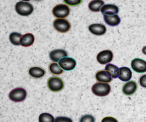
  $1500$ image pairs are evaluated at frame rate 500 f.p.s. The bubbles are detected with a novel convolutional neural network (CNN) based bubble identification algorithm, which is trained to segment bubbles in crowded situations (coloured patches in figure 2b). Furthermore, the hidden part of a partly occluded bubble is estimated with an additionally trained neural network. For this, equal numbers of radial rays are generated for the identified segments, starting from the segment centre to its boundary (green and red lines in figure 2c). Afterwards, radial rays that touch neighbouring segments (red lines in figure 2c) are corrected with the neural network in order to account for the occluded part of the bubble. These steps are illustrated in figure 2, and we refer the reader to Hessenkemper et al. (Reference Hessenkemper, Starke, Atassi, Ziegenhein and Lucas2022) for more technical detail. Here, we show in figure 3 the example images of detected bubbles with corrected outline for all the six cases. While the SmTap, LaTap and LaPen cases have mostly irregular bubble shapes associating with shape oscillations, the cases SmPen, SmPen+ and LaPen+ have fixed shapes. In all of the cases considered, bubble coalescence or breakup was extremely rare and plays a negligible role in the behaviour of the flow. This could be quantified further by computing the Hinze scale for our cases. However, computing this scale requires measuring the turbulent kinetic energy dissipation rate, and this cannot be done reliably using our current experimental set-up.

Figure 2. (a) Example image of the bubbles from a fragment in the middle of figure 3(b), identified by the area marked with white dashed line there for the LaTap case. (b–d) Three steps to reconstruct hidden bubble parts for an irregular shaped bubble: (b) segmentation mask, (c) radial distances, and (d) corrected radial distances.

Figure 3. Example images of the bubbles with fitted contours for an arbitrary instant. (a,c,e) Smaller bubbles with (a) case SmTap, (c) case SmPen and (e) case SmPen+. (b,d,f) Larger bubbles with (b) case LaTap, (d) case LaPen and (f) case LaPen+. The area enclosed by the white dashed line in (b) corresponds to the region shown in figure 2.
The bubble size is calculated using the volume-equivalent bubble diameter of a spheroid as  $d_p=(d_{maj}^2 d_{min})^{1/3}$, where $d_{maj}$ and $d_{min}$ are the lengths of the major and minor axes of the fitted ellipse, respectively. We observe that the surfactant changes the bubble shape dramatically. For the smaller bubbles with $C_\infty =1000$, the shape is close to a sphere with a small aspect ratio $\chi =d_{maj}/d_{min}=1.2$, while for the tap water case, i.e. $C_\infty =0$, we obtain $\chi =1.8$. For the larger bubbles, we also have aspect ratios in a similar range, with $\chi$ decreasing from $1.8$ to $1.3$ when going from higher to lower surfactant concentrations.
After the bubble detection, the centroids are tracked in each image pair to obtain corresponding bubble velocities. Again, a shallow DoF is used, which allows us to select only sharp bubbles in the column centre by evaluating the grey value derivative along their contour. We choose a grey value derivative threshold that provides a centre region of approximately 15 mm thickness ( $3d_p\unicode{x2013}4d_p$) in which the bubbles are evaluated. Some of the important bubble properties are listed in table 1.
It should be noted here that in the case of ellipsoidal bubbles, i.e. the tap water cases, errors in the determined size are larger due to the bubbles being tilted with respect to the camera. This error can result in a bubble size overprediction of up to  $25\,\%$ for a strongly tilted spheroidal bubble with fixed shape, which is, however, on average much lower due to the normal distribution of the orientation angle with a maximum approximately zero (Bröder & Sommerfeld Reference Bröder and Sommerfeld2007). Using the single-bubble data with two cameras (separate experiments reported in § 3.2), we estimate the overprediction of the average volume-equivalent diameter for a fixed spheroidal-shaped bubble (corresponding to case SmTap) to be approximately $4\,\%$. Due to the irregular (wobbling) bubble surfaces, the error for the larger bubbles in the LaTap case are unknown, but we expect it to be of the same order of magnitude. The error for the void fraction is approximately 5 %–8 % (Hessenkemper et al. Reference Hessenkemper, Starke, Atassi, Ziegenhein and Lucas2022), and the error of the bubble velocity is approximately $4\,\%$.
3. Surfactant properties and single-bubble behaviour
3.1. Surfactant properties
The effect of surfactants on the bubbles arises fundamentally due to their impact on the shear stress at the gas–liquid interface, and depends upon the species of surfactants along with their concentration. The variety of surfactants is huge, and our quantitative understanding of their effect on the base fluid is still in its infancy. There are also sometimes ‘untypical’ scenarios reported. Ybert & di Meglio (Reference Ybert and di Meglio1998) showed the effect of surfactant desorption, leading to a remobilization of the interface by considering bubbles contaminated with sodium dodecyl sulfate (SDS). This surfactant has a significant desorption velocity, and they found that due to the progressive remobilization of the interface, the rise velocity of the SDS-preloaded bubble increases over a large portion of its trajectory (see their figure 12), until reaching a constant value. Similar phenomena were also reported by the same authors (Ybert & di Meglio Reference Ybert and di Meglio2000) for short-chain alcohols, where they illustrated bubble rise velocities in ethanol–water solution that were almost indistinguishable from those in pure water, because of its fast desorption kinetics.
In the present study, we focus on the limit of high bubble Péclet number ( $Pe=d_p\,\|\boldsymbol {U}^G\|/D$, where $d_p$ is the bubble diameter, $\boldsymbol {U}^G$ is the averaged bubble velocity, and $D$ is the diffusion coefficient of the surfactant in the liquid), relatively low surfactant concentration compared to the critical micelle concentration (above which surfactants can spontaneously aggregate to form micelles, and the surface tension remains constant) and low rate of desorption. Under these conditions, surface convection is dominant compared to the adsorption–desorption kinetics and diffusive transport of surfactants on the bubble surface. Surfactants collect in a stagnant cap at the back end of the bubble, while the front end is stress-free and mobile. Palaparthi et al. (Reference Palaparthi, Papageorgiou and Maldarelli2006) call this the ‘stagnant cap regime’ – that most commonly realized in typical cases of bubbles moving in a contaminated solution; in this regime, the bubbles are affected significantly by the surfactant, as shown by numerical and experimental results of the rise velocity and wake structure.
In our experiments we use 1-Pentanol as the surfactant and use bulk concentrations  $C_\infty =0$, 333 and 1000 ppm for the six bubble swarm cases. Tests for a single bubble rising in the column were also conducted with concentrations up to 2000 ppm (discussed in § 3.2). Here, the main reason for choosing 1-Pentanol is that with this surfactant (and these concentrations), the bubbles adapt very quickly to the surfactants and no transitions in their motion type appear within the FOV (Tagawa et al. Reference Tagawa, Takagi and Matsumoto2014).
We measure the surface tension separately with a bubble pressure tensiometer, allowing a dynamic determination of the surface tension. For 1-Pentanol concentration 1000 ppm, using profile analysis tensiometry (Eftekhari et al. Reference Eftekhari, Schwarzenberger, Heitkam, Javadi, Bashkatov, Ata and Eckert2021) we observe a surface tension reduction  ${\sim }7\,\%$ compared to tap water. For $C_\infty =333$ ppm, the reduction is ${\sim }2.3\,\%$, which we estimate using linear interpolation (valid at these concentrations; see Cheng & Park Reference Cheng and Park2017). The Péclet number is of the order of $10^5$, indicating that the convection time scale is very small compared to the time scale of the diffusion on the bubble surface. The solubility for 1-Pentanol is 2500 mol m $^{-3}$, which is much higher than the present cases (1000 ppm ${\sim } 9.19\,{\rm mol}\,{\rm m}^{-3}$). Micelles do not form in the bulk aqueous phase, as indicated by the fact that the bubble terminal velocity remains unchanged when $C_\infty$ is increased further (i.e. no surface remobilization has occurred), to be reported later for a single bubble.
3.2. Preliminary test for single bubble
To provide reference cases later for the bubble swarms analysis, we first examine the effect of the surfactants on an isolated bubble in the same set-up by varying the concentration of 1-Pentanol  $C_\infty$ with levels 0, 333, 666, 1000, 1500 and 2000 ppm in tap water. This is a wider range than that used for the bubble swarms to check if any interface remobilization occurs at high concentration. We use a single sparger in the column centre, but vary two types of sparger sizes for each $C_\infty$, which are also used for the bubble swarm results to generate (approximately) two bubble sizes. Here, we generate single bubbles continuously by setting a small gas flow rate as we also did in our previous investigation (Hessenkemper et al. Reference Hessenkemper, Ziegenhein, Lucas and Tomiyama2021a). The low generation frequency of 1 Hz ensures a large enough distance between successive bubbles to avoid any influence from a leading bubble, but allows us to study multiple same-sized bubbles under the same conditions for better statistics.
For the evaluation of the single-bubble rising trajectory in three-dimensions, we conducted stereoscopic measurements with an additional second camera of the same type placed perpendicular with respect to the imaging direction of the first camera. The single-bubble images are also captured with frame rate 500 f.p.s., but with larger f-stop  $11$, since sharp bubble outlines at all depth positions are required. As no overlapping bubbles have to be distinguished in the single-bubble experiments, we use a conventional image processing approach here instead of the CNN-based one that is used for bubble swarms. At first, sharp edges marking the outline of the bubbles are detected with a Canny edge detector. The solid of revolution is then used to determine the volume of the bubble by half rotating the left and right halves of the bubble that is split by the vertical rotation centre of a two-dimensional bubble projection. Afterwards, the volumes of the two camera perspectives are averaged to minimize the remaining perspective errors. Further geometric properties, such as the bubble major axis, defined as the largest extent in a two-dimensional projection, and the bubble minor axis, defined as the largest extent perpendicular to the bubble major axis, are also extracted from the bubble projections (Ziegenhein & Lucas Reference Ziegenhein and Lucas2017). In comparison to the usual approach of fitting ellipses around the contour of detected bubbles, almost the same volume and semi-axis length are obtained, with only minor deviations for irregular-shaped bubbles (Ziegenhein & Lucas Reference Ziegenhein and Lucas2019). Afterwards, the centroid of the bubble projections is tracked through successive images to obtain time-resolved instantaneous bubble velocities $\tilde {\boldsymbol {u}}^G$, which can be decomposed into a ensemble-averaged part $\boldsymbol {U}^G$ and a fluctuating part $\boldsymbol {u}^G$. The same decomposition is also used for the liquid phase with $\tilde {\boldsymbol {u}}^L=\boldsymbol {U}^L+\boldsymbol {u}^L$ in later sections.
Figure 4(a) shows the bubble diameters using two types of sparger size as a function of  $C_\infty$. The bubble size is reduced slightly when adding 1-Pentanol for both types of sparger, generating smaller bubbles from 2.9 mm ( $C_\infty =0$ ppm) to 2.7 mm ( $C_\infty =1000$ ppm), and larger bubbles from 4.4 mm ( $C_\infty =0$ ppm) to 4.1 mm ( $C_\infty =1000$ ppm). This is due to the influence of the surfactants that reduce the surface tension and hence affect the bubble formation at the rigid orifice (Loubière & Hébrard Reference Loubière and Hébrard2004; Drenckhan & Saint-Jalmes Reference Drenckhan and Saint-Jalmes2015). A similar trend can also be found in table 1 for the corresponding bubble swarm cases. In contrast to bubble size, the bubble shape changes dramatically (figure 4b), with the aspect ratio reducing from $1.8$ at 0 ppm to $1.15$ at 1000 ppm for the smaller bubble, and $1.9$ at $0\,\mathrm {ppm}$ to 1.36 at $1000\,\mathrm {ppm}$ for the larger bubble. Further increasing $C_\infty$ does not change the bubble shapes for the present smaller and larger bubbles. A similar trend can be found for the averaged rise velocity $U^G_1$ for the both bubble sizes, namely, increasing 1-Pentanol concentration above 1000 ppm does not affect $U^G_1$. For both bubble sizes and for all concentrations considered, we found no increase of the rise velocity, nor any change in terms of aspect ratio above $C_\infty =1000$ ppm, hence no surface remobilization has occurred. Based on these, we assume that for both bubble sizes, a saturated contamination state (at least from the hydrodynamic perspective) is reached at the threshold $C_\infty \approx 1000$ ppm.

Figure 4. Measured single-bubble (a) size, (b) aspect ratio and (c) rise velocity in different 1-Pentanol concentrations.
We now look more in detail at the single-bubble cases with  $C_\infty =0$, $333$ and $1000$ ppm, since they have the same set of $C_\infty$ values as the swarm cases that we will discuss later. We label these cases S-SmTap, S-SmPen and S-SmPen+ for the smaller bubble, and S-LaTap, S-LaPen and S-LaPen+ for the larger bubble, respectively (where the first letter S denotes a single bubble). Figure 5(a) shows a three-dimensional view of the bubble trajectories for the three smaller bubble cases, while figure 5(b) shows a view of these trajectories from the top. The trajectories are similar to those found by Tagawa et al. (Reference Tagawa, Takagi and Matsumoto2014) for 2 mm bubbles, with helical trajectories at lower 1-Pentanol concentration (see S-SmTap and S-SmPen), and zigzag rising paths for higher concentration (S-SmPen+). These zigzag and helical motions are accompanied by oscillations in the vertical velocity $\tilde {u}^G_1$ plot of figure 5(c) (corresponding to the paths in figure 5a), i.e. the bubbles alternately speed up and slow down as they rise. As expected, the S-SmPen+ case has much higher oscillation in $\tilde {u}^G_1$, compared to the S-SmTap and S-SmPen cases. This is caused by the relatively unstable wake structure that is associated with zigzag paths, rather than the more stable one associated with the helical trajectories (Cano-Lozano et al. Reference Cano-Lozano, Martinez-Bazan, Magnaudet and Tchoufag2016). Moreover, we observe that the helical trajectories of S-SmTap and S-SmPen are not as regular as those in Tagawa et al. (Reference Tagawa, Takagi and Matsumoto2014) due to our larger bubble size ${\sim }3$ mm. This is also indicated by the vertical velocities (figure 5c), showing oscillations in S-SmTap and S-SmPen compared to the constant $\tilde {u}^G_1$ for the cases with relatively perfect helical rising paths in Tagawa et al. (Reference Tagawa, Takagi and Matsumoto2014). The characteristic diameters of the helical paths in both cases are close to 10 mm, which is similar to that found in Riboux et al. (Reference Riboux, Risso and Legendre2010) for a 2.5 mm bubble rising in tap water. This characteristic diameter is much smaller than the depth of the present column, so the side-wall effects are negligible in the experiment.

Figure 5. (a) Three-dimensional trajectories and (b) their top view, and corresponding instantaneous bubble velocities with components (c)  $\tilde {u}^G_1$, (d) $\tilde {u}^G_2$ and (e) $\tilde {u}^G_3$ over time (normalized by $\Delta t=2$ ms) of smaller single bubbles at $C_\infty =0$ ppm (S-SmTap), $C_\infty =333$ ppm (S-SmPen) and $C_\infty =1000$ ppm (S-SmPen+). All plots are from the same track of the particular case.
Another important observation from figures 5(c–e) is that the frequency of the vertical velocity is approximately twice as large as that of the horizontal velocities due to the frequency of the force oscillations in the corresponding directions (Mougin & Magnaudet Reference Mougin and Magnaudet2006). Moreover, there is a trend that with increasing  $C_\infty$, the frequency of the oscillation in velocities increases. This is in line with the observation reported in Tagawa et al. (Reference Tagawa, Takagi and Matsumoto2014) for their smaller bubbles.
In figure 6, we plot the same quantities for the three larger bubble cases. A fixed path type cannot be found for case S-LaTap. Although in figure 6(e) it shows a zigzagging trend, there are many other snapshots showing a flattened helix (not shown here). Case S-LaTap belongs to the chaotic regime due to the very large  $Re_p$ and $Eo$, while S-LaPen exhibits a flattened helical motion, and S-LaPen+ converges towards a zigzag path. Moreover, compared to the smaller bubbles, the vertical velocities (figure 6a) in all three larger bubble cases display irregular oscillations.

Figure 6. (a) Three-dimensional trajectories and (b) their top view, and corresponding instantaneous bubble velocities with components (c)  $\tilde {u}^G_1$, (d) $\tilde {u}^G_2$ and (e) $\tilde {u}^G_3$ over time (normalized by $\Delta t=2$ ms) of larger single bubbles at $C_\infty =0$ ppm (S-LaTap), $C_\infty =333$ ppm (S-LaPen) and $C_\infty =1000$ ppm (S-LaPen+). All plots are from the same track of the particular case.
4. Flow characterization for bubble swarm
Basic statistics of both phases for the considered cases are plotted in figure 7. Both the void fraction (figure 7a) and the vertical gas/liquid velocity (figure 7b) have very flat profiles, indicating statistical homogeneity of the current flow in the FOV. Even with zero bulk flow (averaged over the entire flow cross-section), we observe for almost all the cases  $U^L_1\neq 0$ along the horizontal axis of the FOV (especially for the cases SmPen+ and LaPen+), so that the relative velocity in the FOV is in general not equal to the bubble terminal rise velocity. Furthermore, due to the Marangoni effect, we find that the bubble swarms rise more slowly with increasing $C_\infty$ for both smaller and larger bubbles, consistent with our results for the corresponding single bubble in § 3.2. It is worth noting that although LaPen and LaPen+ have a similar $U^G_1$, LaPen+ has a smaller relative velocity due to the higher $U^L_1$, as indicated by its smaller bubble Reynolds number (table 1).

Figure 7. (a) Gas void fraction and (b) liquid/gas vertical velocity along the horizontal axis of the FOV.
We now turn to consider the role played by the surfactant in generating BIT. Hereafter, all average quantities refer to the liquid, so that the upper index  $L$ is dropped for simplicity. In figure 8(a), we plot the turbulent kinetic energy (TKE) $k$, calculated as
 \begin{equation} k=\tfrac{1}{2}\left ( (u_1^{rms})^2+2(u_2^{rms})^2\right ),\end{equation}
assuming that the out-of-plane velocity variance is equal to the measured horizontal component. This approximation – axisymmetry about the vertical direction – is expected for the BIT dominated flows far from the wall. Here,  $u_1^{rms}$ and $u_2^{rms}$ are the root-mean-square values of the vertical and horizontal velocity fluctuations, respectively. For both smaller and larger bubbles, surprisingly, the TKE is highest for the cases with the highest $C_\infty$, although SmPen+ and LaPen+ have the lowest $Re_p$ in the cases of smaller and larger bubbles, respectively. It is also interesting to note that TKE in the cases SmPen and LaPen does not change much compared to SmTap and LaTap, respectively, indicating that the amount of 1-Pentanol added ( $C_\infty =333$ ppm) is not enough to modify the BIT already initiated in the tap water system. However, we should keep in mind that the bubble sizes in SmPen and LaPen are slightly smaller than their corresponding tap water cases (see table 1), so that if the TKE is almost the same for the $C_\infty =0$ and $C_\infty =333$ ppm cases, then the surfactant is in fact leading to a positive contribution to the BIT generation.

Figure 8. (a) Turbulent kinetic energy along the horizontal axis of the FOV. (b) Reynolds number  $Re_{H_2}$ plotted versus large-scale anisotropy ratio $u_1^{rms}/u_2^{rms}$.
In table 2, we summarize the effect of the surfactant on three aspects that influence BIT. Aside from reducing the bubble Reynolds number, the bubble surface instability (e.g. deformation and wobbling) also reduces when increasing  $C_\infty$, and both of these reductions have a negative impact on BIT production. This suggests that the change of boundary condition induced by increasing $C_\infty$ plays the key role in causing the TKE to be enhanced by the addition of surfactants. Following our previous study (Ma et al. Reference Ma, Ott, Fröhlich and Bragg2021), we define a Reynolds number $Re_{H_2}\equiv u^\ast H_2/\nu$, indicating the range of scales in the turbulent bubbly flows. Here, $u^\ast \equiv \sqrt {(2/3)k_{{FOV}}}$, and $k_{{FOV}}$ is the TKE averaged over the FOV of the liquid phase. In figure 8(b), we depict $Re_{H_2}$ versus the large-scale anisotropy ratio $u_1^{rms}/u_2^{rms}$ (also averaged over the FOV). The figure reflects the same behaviour as the TKE, namely the case with the highest $C_\infty$ also has the largest $Re_{H_2}$ for the corresponding bubble size group. Furthermore, we find that for large scales whose fluctuating velocities are characterized by $u_1^{rms}$ and $u_2^{rms}$, the smaller bubbles produce more anisotropy in the flow than the larger bubbles, as reflected by a larger ratio $u_1^{rms}/u_2^{rms}$ for the cases SmTap, SmPen and SmPen+. This is in very close agreement with our previous study based on DNS data of bubble-laden turbulent channel flow driven by a vertical pressure gradient and with no-slip boundary conditions on the bubble surfaces (Ma et al. Reference Ma, Ott, Fröhlich and Bragg2021).
Table 2. Summary of how surfactants modify the bubble Reynolds number, boundary condition and deformability, and the impact (positive or negative) that these modifications will have on the intensity of the turbulence generated by the rising bubbles. The right-hand image in the centre column is a schematic representation of surfactant distribution on the surface of a rising bubble, and the red dashed arrows indicate the Marangoni stress.

The more important point prompted by figure 8(b) is that the large-scale anisotropy increases significantly with increasing surfactant concentration for both smaller and larger bubbles. This behaviour is due to the effect of the surfactant on both the wake structure and trajectory type of the bubbles as  $C_\infty$ changes, as was already seen for different single bubbles in figures 5 and 6. Indeed, these anisotropy results indicate that the increase of TKE due to the addition of surfactants is due mainly to the change of the bubble surface boundary properties, and not due to an increase of the lateral movement, since the results indicate that the lateral motions become weaker compared with the vertical motions as the surfactant concentration is increased. This is in contrast to the case of single buoyant or heavy particles that are rising/settling in liquids where enhanced horizontal motion was found to be the cause of increased liquid velocity fluctuations despite there being a corresponding reduction in particle Reynolds number (Veldhuis, Biesheuvel & Lohse Reference Veldhuis, Biesheuvel and Lohse2009; Horowitz & Williamson Reference Horowitz and Williamson2010; Mathai et al. Reference Mathai, Zhu, Sun and Lohse2018).
In figure 9, the PDFs of the liquid velocity fluctuations (normalized by their standard deviations) are shown for both directions. In agreement with the previous experimental results (Riboux et al. Reference Riboux, Risso and Legendre2010; Lai & Socolofsky Reference Lai and Socolofsky2019), we find that the PDFs of the vertical velocity fluctuations are strongly positively skewed for all the cases, while the PDFs of the horizontal velocities are symmetric. We also find that for the three smaller bubble cases, the PDFs become increasingly non-Gaussian in the order SmPen+, SmPen, SmTap, which corresponds to decreasing  $C_\infty$ (1-Pentanol) and $Re_{H_2}$. By contrast, for the larger bubble cases, the dependence of the PDFs on $C_\infty$ is very weak. Explanations for the observed behaviour will be considered in the next section.

Figure 9. Normalized PDFs of liquid velocity fluctuations: (a,b) the three smaller bubble cases, and (c,d) the three larger bubble cases.
5. Turbulence modification across scales
5.1. Turbulence anisotropy
The components of the second-order velocity structure function are defined as
 \begin{equation} D_2^{ij}(\boldsymbol{x},\boldsymbol{r},t)\equiv\langle \Delta u_i(\boldsymbol{x},\boldsymbol{r},t)\,\Delta u_j(\boldsymbol{x},\boldsymbol{r},t)\rangle, \end{equation}
where  $\Delta u_i(\boldsymbol {x},\boldsymbol {r},t)$ denotes the difference in the velocity at positions $\boldsymbol {x}$ and $\boldsymbol {x}+\boldsymbol {r}$ at time $t$, and $\langle {\cdot } \rangle$ denotes an ensemble average. Hereafter, we suppress the space $\boldsymbol {x}$ and time $t$ arguments since we are considering a flow that is statistically homogeneous and stationary over the FOV. The calculation of liquid velocity increments in a bubbly flow is somewhat delicate, since the liquid velocity is not defined at points occupied by a bubble. To overcome this non-continuous velocity signal challenge, the statistics of the velocity increments were computed based only on lines of grid points spanning the FOV at time instants where none of the points on the line were occupied by a bubble. A more detailed discussion of this method can be found in Ma et al. (Reference Ma, Ott, Fröhlich and Bragg2021, Reference Ma, Hessenkemper, Lucas and Bragg2022).
The PSV measurement provides access to data associated with separations along two directions, namely, the vertical separation  $\boldsymbol {r}=r_1\boldsymbol {e}_1$ ( $r_1=\|\boldsymbol {r}\|$) and the horizontal separation $\boldsymbol {r}=r_2\boldsymbol {e}_2$ ( $r_2=\|\boldsymbol {r}\|$). Hence we are able to compute the four contributions $D^L_2(r_1)=D_2^{11}(r_1)$, $D^L_2(r_2)=D_2^{22}(r_2)$, $D^T_2(r_1)=D_2^{22}(r_1)$ and $D^T_2(r_2)=D_2^{11}(r_2)$ based on the Cartesian coordinate system depicted in figure 1.
Figures 10(a) and 10(b) show the measured transverse and longitudinal second-order structure functions of the  $u_1$ component, respectively. The results show that the values of the structure functions increase in the order SmTap, SmPen, SmPen+, LaTap, LaPen, LaPen+, which corresponds to larger bubble size and higher surfactant concentration. This ordering also holds for the $u_2$ component computed (not shown). Similar to the results for the TKE, while the difference between Sm(La)Tap and Sm(La)Pen is small, $D_2^{\gamma \gamma }$ (no index summation is implied for $\gamma$) for Sm(La)Pen+ have noticeably higher values across most scales for both smaller and larger bubble sizes. The plot shows the $r^{2/3}$ scaling that would be expected for single-phase HIT according to Kolmogorov's 1941 theory (Pope Reference Pope2000). The results show that for the bubbly turbulent flows in our experiments, an extended $r^{2/3}$ scaling regime does not occur in any range of separations. At smaller separations, the structure functions exhibit behaviour consistent with a dissipation range, e.g. $D_2^{11}(r_1)\propto r_1^2$. However, our experimental resolution is not fine enough to determine whether this really does correspond to dissipation range scaling, or whether this scaling is caused by other effects in the flow (including the frequency of wake oscillations), and that the true dissipation range occurs at separations smaller than we can resolve. Moreover, since there is no inertial range in the flow, there is no way to estimate the energy dissipation rate based indirectly on the structure functions, as is often done in other contexts.

Figure 10. (a) Transverse and (b) longitudinal second-order structure functions of the  $u_1$ component, with separations along the (a) horizontal and (b) vertical directions. The black dashed lines indicate slope $r^{2/3}$.
To characterize the multiscale anisotropy associated with  $D_2^{ij}$, we plot the ratios of components $D^L_2(r_1)/D^L_2(r_2)$ and $D^T_2(r_2)/D^T_2(r_1)$ in figure 11, which would be equal to unity for an isotropic flow (Carter & Coletti Reference Carter and Coletti2017). Generally, the results show that both ratios decrease monotonically for decreasing separation. Moreover, the ratio of the transverse structure functions departs more strongly from unity than the longitudinal ones. By comparing the cases with the same bubble size, we find that generally the cases with higher surfactant concentration generate stronger anisotropy in the flow across the scales, and this trend is most obvious in the plot for $D^T_2(r_2)/D^T_2(r_1)$. This is in agreement with the results of the large-scale anisotropy in § 4.

Figure 11. Ratio of (a) longitudinal and (b) transverse structure functions in different separation directions for all the cases. The horizontal lines indicate the value unity.
Furthermore, considering the cases with the same  $C_\infty$, our results indicate that smaller bubbles generate stronger anisotropy in the flow, consistent with our previous studies (Ma et al. Reference Ma, Ott, Fröhlich and Bragg2021, Reference Ma, Hessenkemper, Lucas and Bragg2022) that considered only fully contaminated bubbles. However, the results in figure 11 show that it is not true in general that smaller bubbles generate stronger anisotropy in the flow, because it depends on the surfactant concentration. For example, figure 11 shows that LaPen+ can be more anisotropic than SmTap.
5.2. Extreme fluctuations in the flow
Having explored the role of surfactants on the flow anisotropy, we now turn to consider the effect of surfactants on extreme fluctuations of the velocity increments – a phenomenon associated with internal intermittency in single-phase turbulence (Frisch Reference Frisch1995; Sreenivasan & Antonia Reference Sreenivasan and Antonia1997). In the present bubbly flows, extreme events in the liquid phase result from the boundary of the wakes produced by the bubbles (Ma et al. Reference Ma, Hessenkemper, Lucas and Bragg2022). These contributions can be seen in figure 12, with the normalized velocity increments ( $r_2 = \Delta$, where $\Delta$ is one PSV grid) showing large values at the edge of the wakes, while the velocities are largest inside the wakes. Another possible contribution to extreme events would come from the flow in the boundary layer at the top of the rising bubble where the flow may change abruptly from being equal to the bubble surface velocity to the background bulk velocity over a thin boundary layer. For spherical bubbles with large $Re_p$ rising in a quiescent flow, the thickness of this boundary layer is $O(d_p\,Re_p^{-1/2})$ (Moore Reference Moore1963; Batchelor Reference Batchelor1967). However, we cannot resolve the velocity fluctuations in this thin boundary layer with our current experimental method (and the results discussed below should be interpreted accordingly), and further work is needed to understand how these regions might contribute to extreme fluctuations in the flow.

Figure 12. (a) Snapshot of the original velocity vector. (b) Intensity distributions of the normalized velocity increment  $|\Delta u_1(r_2=\varDelta ) |/\sigma _{\Delta u_1}$from the same instant based on the SmPen+ case. The in-focus bubbles are denoted in (a).
In figure 13, we plot the PDFs of the velocity increments for separations equal to ten PSV grids  $(r=10\varDelta =0.18H_2)$, corresponding to an ‘eddy size’ with $O(d_p)$. (The results for other separations show qualitatively similar trends and so are not shown.) First, all of the six cases show that the velocity increments have strongly non-Gaussian PDFs, just as in single-phase turbulence. Second, while the PDFs of the transverse velocity increments in figures 13(c,d) are almost symmetric, the PDFs of the longitudinal velocity increments in figures 13(a,b) are negatively skewed for the horizontal separations $r_2$. Finally, with respect to the effect of bubble size and surfactant concentration, the results show very interesting behaviours: for the smaller bubbles, both the longitudinal and transverse PDFs (figures 13a,c) become increasingly non-Gaussian in the order SmPen+, SmPen, SmTap, which corresponds to the order of decreasing $C_\infty$ of 1-Pentanol. This is consistent with our previous finding (Ma et al. Reference Ma, Hessenkemper, Lucas and Bragg2022) that the non-Gaussianity of the PDFs of the velocity increments becomes stronger as the Reynolds number (here, $Re_{H_2}$) is decreased in bubble-laden turbulent flow considered here, while the opposite occurs for single-phase turbulence (Frisch Reference Frisch1995). An explanation for why the intermittency is largest for the cases with lower surfactant concentration can be given as follows. For these three cases, the volume fraction is not large, and there are relatively few regions in the flow where turbulence is produced due to the bubble wakes, meaning that turbulence in the flow is very patchy and therefore intermittent. For the cases with higher $C_\infty$, they have larger flow Reynolds numbers accompanied by longer and wider bubble wakes. As a result, the wake regions are more space filling and hence the flow is less intermittent than the cases with lower surfactant concentration, which have shorter and narrower bubble wakes. Again, this difference compared to intermittency in single-phase turbulence can be traced back to the fact that the regions of intense small-scale velocity increments occur near the turbulent/non-turbulent interface at the boundary of the bubble wake, which is more similar to so-called external intermittency (Townsend Reference Townsend1949) than internal intermittency.

Figure 13. Normalized PDFs of the (a,b) longitudinal and (c,d) transverse velocity increments for (a,c) the three smaller bubble cases and (b,d) three larger bubble cases, with the separations along the horizontal direction ( $r_2= 10\varDelta$, where $\varDelta$ is one PSV grid).
The  $C_\infty$ dependency of the small-scale intermittency just discussed for the smaller bubbles is, however, much weaker for the larger bubbles (figures 13b,d). A potential reason for this difference is that the three larger bubble cases have volume fractions that are almost three times larger than those for the smaller bubbles, and the bubble wake volume is also much larger, with much higher turbulence intensity generated by the wakes. As a result of these properties, while there are significant regions of the flow that are almost quiescent for the smaller bubble cases, the same is not true for the larger bubbles, with turbulent activity filling a significant fraction of the flow. Due to this, the velocity difference in and outside the wake is smaller for the larger bubble cases than the smaller bubble cases, and the intermittency is less dependent on $C_\infty$ since even for the largest $C_\infty$ case, these velocity differences across the wake boundaries are already smaller. This then explains why LaTap, LaPen and LaPen+ do not show the same $C_\infty$ dependence in the PDFs as the smaller bubble cases.
While the PDF results present the effect of the surfactants on the extreme events at a fixed separation, we look at now this property across all the scales quantified by the kurtosis  $D^T_4(r_2)/(D^T_2(r_2))^2$ and $D^L_4(r_2)/(D^L_2(r_2))^2$ (figure 14). The first observation from the results in figure 14 is that all six bubble-laden cases show a similar behaviour as $r$ increases, with values of up to 30 gradually reducing as $r$ increases. However, there is still considerable deviation from the Gaussian value of 3 even at the largest scale $r_2/H_2=1$. For both the transverse and longitudinal components, the kurtosis is larger for the cases with smaller bubbles, reflecting the same trend as the PDFs of the velocity increments at the single scale $r_2=10\varDelta$ (see figures 13(a,b) or 13(c,d)). The qualitative effect of the surfactant concentration on the extreme events as quantified by the PDF results for $\Delta \boldsymbol {u}(r_2=10\varDelta )$ (figure 13) can be extended to almost all the scales. While the kurtosis decreases in the sequence SmTap, SmPen to SmPen+ across the scales of the flow, the values of the three cases with larger bubbles are very similar.

Figure 14. Normalized fourth-order (a) transverse and (b) longitudinal structure functions, corresponding to the kurtosis of the velocity increments along the horizontal direction. The horizontal lines indicate the Gaussian value of  $3$ for the kurtosis.
In table 3, we show the values of the kurtosis of  $u_1$ and $u_2$ as well as those of $\Delta u_1$ and $\Delta u_2$ at large separations in order to understand how the non-Gaussianity of the velocity increments relates to the non-Gaussianity of the velocity fluctuations observed in figure 9. Since the largest separations that we can observe are constrained by the FOV, we also compute the theoretical values of the kurtosis of $\Delta u_1$ and $\Delta u_2$ at infinite separation, assuming that the flow is homogeneous. These theoretical expressions are evaluated from the definitions of the structure functions using the fact that at infinite separations, the velocities at two points are uncorrelated. The resulting expressions are
 $$\begin{gather} \lim_{r_2/H_2\to\infty}\frac{D^T_4(r_2)}{[D^T_2(r_2)]^2}= \frac{1}{2}\,\frac{\langle u_1 ^4\rangle}{\langle u_1^2\rangle^2}+\frac{3}{2}, \end{gather}$$
 $$\begin{gather}\lim_{r_2/H_2\to\infty}\frac{D^L_4(r_2)}{[D^L_2(r_2)]^2}=\frac{1}{2}\,\frac{\langle u_2^4\rangle}{\langle u_2^2\rangle^2}+\frac{3}{2}. \end{gather}$$
If  $u_1$ and $u_2$ have Gaussian distributions, then the kurtosis of $u_1$ and $u_2$ is equal to 3, as is the kurtosis of $\Delta u_1$ and $\Delta u_2$ at $r_2/H_2\to \infty$. However, for non-Gaussian $u_1$ and $u_2$, the kurtosis values for $u_1$ and $u_2$ are not equal to those for $\Delta u_1$ and $\Delta u_2$ at $r_2/H_2\to \infty$.
Table 3. Comparison between the kurtosis of the fluctuating velocity and the kurtosis of the velocity increment at large scale. Also shown is the theoretical kurtosis of the velocity increment, which is the value the kurtosis would have at infinite separation in a homogeneous flow.

The values of the kurtosis of  $u_1$ and $u_2$ in table 3 reflect the same trend as those based on the velocity increments: the values are larger for smaller bubbles, and decrease in the sequence SmTap, SmPen to SmPen+, while the kurtosis values for LaTap, LaPen and LaPen+ are similar. The values of the kurtosis of $\Delta u_1$ and $\Delta u_2$ measured at $r_2/H_2\approx 1$ are very close to the theoretical values, indicating that our FOV is sufficiently large to capture the largest scales of the flow.
Finally, in our previous work (Ma et al. Reference Ma, Hessenkemper, Lucas and Bragg2022), we noted that the PDFs of the velocity increments at  $r_2/H_2\approx 1$ are very different from the PDFs of the velocities. This seemed surprising given the expectation that these two PDFs should converge at sufficiently large separations because the correlation of the velocity between the two points vanishes in that limit. We speculated that the lack of convergence of the PDFs was due to our FOV being too small to observe the asymptotic approach of the PDFs at sufficiently large separations. However, the results in (5.2) and (5.3) indicate that our previous expectation of the convergence of these PDFs was in fact mistaken. Indeed, a calculation of other moments shows that more generally, the moments of the velocity increments at large separations will not approach the moments of the velocities unless the velocity fluctuations are Gaussian. Hence it follows that their PDFs will also not approach unless the velocity fluctuations are Gaussian.
6. Conclusions
In this work, we have used experiments to investigate the effect of surfactants on BIT using recently developed PSV and bubble identification techniques for bubble/particle-laden flows. The experiments consider two bubble sizes, 3 and 4 mm, and three different surfactant (1-Pentanol) concentrations for each bubble size. The addition of surfactants changes the bubble shape, as well as the interface boundary condition from a quasi-free-slip condition to a no-slip condition.
To provide some reference cases, we first investigated how 1-Pentanol influences single bubbles in terms of the size of the bubbles formed in the system, the bubble aspect ratios, the bubble rise velocity and the nature of their trajectories. We find that for the two bubble sizes considered, an approximately saturated contamination state is reached at  $C_\infty \approx 1000$ ppm. The effect of the surfactant on the bubble trajectories is similar to that observed in Tagawa et al. (Reference Tagawa, Takagi and Matsumoto2014), with helical trajectories at lower 1-Pentanol concentrations and zigzag rising trajectories for higher concentration for smaller bubble cases. The effect of the surfactant was similar for the larger bubbles, although in the absence of the surfactants, the trajectories of the larger bubbles appear chaotic.
Our results for bubble swarms show that for BIT-dominated flows, the level of anisotropy is strong in general, and not negligible even at small scales in the flow, consistent with previous results. However, our results reveal that for the same bubble size, the flow anisotropy can be strongly enhanced by increasing the surfactant concentration. We also investigated extreme events in the flow by considering the normalized PDFs of the velocity increments at the scale of the bubble size. For the smaller bubbles, the PDFs become increasingly non-Gaussian when the surfactant concentration is decreased. This is consistent with our previous finding that the non-Gaussianity of the PDFs of the velocity increments becomes stronger as the Reynolds number is decreased in the bubble-laden turbulent flows considered here, the opposite of what occurs for internal intermittency for single-phase turbulence, which increases with increasing Reynolds number. However, the dependency of the non-Gaussianity of the velocity increments on the surfactant concentration is much weaker for the cases with larger bubbles. An explanation for this difference is that the larger bubble cases have much larger volume fractions compared to those for the smaller bubbles, and the bubble wake volume is also much larger, with much higher turbulence intensity generated by the wakes. Due to this, the velocity difference in and outside the wake is smaller for the larger bubble cases than the smaller bubble cases, and the intermittency is less dependent on the surfactant concentration.
While this study has focused on the impact of surfactants on the properties of the liquid turbulence in BIT, another important topic is to investigate how the surfactants impact the bubble clusters and bubble dispersion. These will be investigated in a future study.
Acknowledgements
The authors would like to acknowledge T. Ziegenhein for much technical support in the experimental method over the years. T.M. benefited from fruitful discussions on this topic with J. Fröhlich, Y. Liao, P. Shi, S. Heitkam, K. Schwarzenberger, X. Xu, Y. Tagawa and G. Katul.
Declaration of interests
The authors report no conflict of interest.
Data availability
The data that support the findings of this study are available from T.M. on request.


 Open access