


1. Introduction
Resolvent analysis (also called input/output analysis or frequency response analysis) is a powerful and popular tool for studying linear energy-amplification mechanisms within the Navier–Stokes equations. The resolvent operator is derived from the linearized Navier–Stokes equations and constitutes a transfer function between inputs and outputs of interest. It has been used to study the linear response of flows to external excitation (Trefethen et al. Reference Trefethen, Trefethen, Reddy and Driscoll1993; Farrell & Ioannou Reference Farrell and Ioannou2001; Jovanović & Bamieh Reference Jovanović and Bamieh2005; Sipp et al. Reference Sipp, Marquet, Meliga and Barbagallo2010) and to forcing from the nonlinear terms in the Navier–Stokes equations (McKeon & Sharma Reference McKeon and Sharma2010). In the latter context, the method can be derived by reorganizing the Navier–Stokes equations into terms that are linear and nonlinear with respect to perturbations to a laminar base flow or a turbulent mean flow. The singular value decomposition (SVD) of the resolvent operator associated with the linearized Navier–Stokes equations then identifies modes that are optimal in terms of their linear gain between the nonlinear terms (thought of as an input) and the perturbations to the mean (output). These optimal modes can be used to study worst-case transition scenarios for laminar flows (Monokrousos et al. Reference Monokrousos, Åkervik, Brandt and Henningson2010) and have been shown to provide a useful model of coherent structures within turbulent flows. In particular, resolvent modes provide an approximation of the space–time coherent structures educed from data using spectral proper orthogonal decomposition (Towne, Schmidt & Colonius Reference Towne, Schmidt and Colonius2018).
While there are variations in the approaches, a typical procedure for computing resolvent modes involves (i) discretization of the continuous flow problem to obtain a finite-dimensional one, (ii) representing the linearized relationship between inputs and outputs as a matrix (the resolvent operator), and (iii) finding one or more singular values/vectors of the resolvent matrix via SVD.
The computational resources required to compute resolvent modes depend critically on the number of spatial dimensions that must be numerically discretized. The linearized Navier–Stokes equations nominally contain three spatial dimensions, but the equations can be simplified by expanding the flow variables into Fourier modes in homogenous dimensions, i.e. directions in which the base flow (about which the equations are linearized) does not vary. This drastically reduces the size of the discretized operators that must be manipulated, decreasing the computational cost of the model. Methods in which all inhomogeneous dimensions are discretized are often called global methods (Theofilis Reference Theofilis2011).
Computing global resolvent modes for flows with more than one inhomogeneous direction remains a computationally intensive task (Jovanović Reference Jovanović2021). Whereas flows with one inhomogeneous direction can now be tackled on a laptop computer, high-memory workstations and large-scale clusters must be employed for flows with two and three inhomogeneous directions, respectively (Taira et al. Reference Taira, Brunton, Dawson, Rowley, Colonius, McKeon, Schmidt, Gordeyev, Theofilis and Ukeiley2017). These requirements limit the utility of global resolvent analysis for many flows of interest and mitigate some of their advantages compared with fully nonlinear numerical simulations.
Recent efforts to reduce the cost of resolvent analysis have focused on reducing the cost of computing the SVD of the resolvent operator. For example, Moarref et al. (Reference Moarref, Jovanović, Tropp, Sharma and McKeon2014) used a randomized singular value decomposition (RSVD) algorithm to compute resolvent modes for a turbulent channel flow (which has only one inhomogeneous direction) and reported that this reduced the cost of the calculations by a factor of two. Ribeiro, Yeh & Taira (Reference Ribeiro, Yeh and Taira2020) offered several improvements for the application of RSVD to resolvent analysis and achieved an order-of-magnitude speedup compared with standard SVD algorithms for a separated flow around an airfoil (which has two inhomogeneous directions). Given the reduced cost of computing the SVD, the majority of the remaining cost in their algorithm is associated with computing the action of the resolvent operator on a vector. This requires solution (inversion) of the linear system, which is typically accomplished using lower–upper (LU) decomposition. The computation rate and memory bottlenecks of this step limit the grid sizes of such solutions and/or force them to be performed in a high-performance-computing environment. Computing the action of the resolvent operator on a vector is also the limiting factor for time-stepping methods (Monokrousos et al. Reference Monokrousos, Åkervik, Brandt and Henningson2010; Farghadan et al. Reference Farghadan, Towne, Martini and Cavalieri2021; Martini et al. Reference Martini, Rodríguez, Towne and Cavalieri2021), where the dominant cost is integrating direct and adjoint linear equations in the time domain used to apply the resolvent operator and its adjoint. As typically one aims to characterize the input/output relationships over a broad range of frequencies and parameters, it is of great interest to reduce the computational burden of resolvent analysis.
In this paper we develop a method that significantly reduces the cost of computing resolvent modes for flows that include a slowly varying spatial direction, i.e. a direction in which the mean flow is inhomogeneous but changes gradually. This common class of flows includes free-shear flows like mixing layers and jets as well as wall-bounded flows with spatially developing boundary layers on gradually changing objects like a flat plate, cone, airfoil, etc. First, we show how the action of the resolvent operator on a forcing vector can be efficiently and accurately approximated for slowly varying flows using a well-posed spatial marching technique. Second, we show how this capability can be used to compute the singular modes of the resolvent operator using iterative downstream and upstream marching at significantly reduced computational cost, especially in terms of memory requirements.
Spatial marching methods are commonly applied to slowly varying flows in order to compute approximate eigenmodes or the downstream response to an initial disturbance introduced at some upstream location. The classical tool for these purposes is the parabolized stability equations (PSE), which constitute an ad hoc generalization of classical parallel-flow stability theory (Bertolotti, Herbert & Spalart Reference Bertolotti, Herbert and Spalart1992; Herbert Reference Herbert1997). The basic idea of PSE is to separate the flow variables at each frequency into a slowly varying shape function and a rapidly varying wave-like component. Inserting this ansatz into the linearized Navier–Stokes equations leads to a modified set of equations for the shape function, which can be rapidly solved via spatial integration in the slowly varying direction, leading to an approximation of the downstream response to an initial disturbance. The initial disturbance is usually chosen to be a locally parallel eigenmode, in which case the PSE solution is interpreted as a weakly non-parallel eigenmode of the flow or as the response to a localized forcing designed to generate that mode at the domain inlet.
Several authors have recently observed that for flows dominated by a single convective instability, the PSE solution appears to provide a reasonable approximation of the leading resolvent output mode, i.e. the left singular vector of the resolvent operator with the largest singular value (Beneddine et al. Reference Beneddine, Sipp, Arnault, Dandois and Lesshafft2016; Jeun, Nichols & Jovanović Reference Jeun, Nichols and Jovanović2016). However, there are several issues that limit the utility of PSE for approximating resolvent modes. First, PSE does not provide any information about the input resolvent modes or gains, both of which are critical for analysis and modelling. Second, PSE can accurately capture the influence of only a single instability mechanism. This limitation stems from the fact that, despite their name, the parabolized stability equations are, in fact, elliptic in the slowly varying direction due to the boundary value nature of the linearized Navier–Stokes equations (Li & Malik Reference Li and Malik1997). As a result, the PSE spatial integration is mathematically ill-posed, and regularization methods are required to stabilize the spatial march. Recently, Towne, Rigas & Colonius (Reference Towne, Rigas and Colonius2019) showed that these regularization methods contaminate the PSE solution, except in cases where the flow is dominated by a single instability mode at each frequency. As a result, PSE is not an appropriate tool for flows in which multiple modes are of interest, including multiple instability mechanisms, transient growth or acoustics.
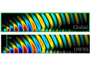
Towne & Colonius (Reference Towne and Colonius2015) introduced an alternative method for obtaining fast, approximate linear solutions for slowly varying flows that overcomes these issues by constructing well-posed spatial evolution equations that do not require detrimental PSE-like regularization. Using ideas originally developed for constructing high-order non-reflecting boundary conditions (Hagstrom & Warburton Reference Hagstrom and Warburton2004), the flow variables are decomposed into upstream- and downstream-travelling waves in the slowly varying direction. An approximate evolution equation is derived for the downstream-travelling waves, which can be solved via a well-posed spatial march. The method, which has come to be known as the one-way Navier–Stokes (OWNS) equations, has been applied to both free-shear flows such as mixing layers (Towne & Colonius Reference Towne and Colonius2013) and jets (Towne & Colonius Reference Towne and Colonius2014; Rigas et al. Reference Rigas, Schmidt, Colonius and Brès2017b) as well as wall-bounded flows (Rigas, Colonius & Beyar Reference Rigas, Colonius and Beyar2017a; Kamal et al. Reference Kamal, Rigas, Lakebrink and Colonius2020) and is typically more than an order-of-magnitude faster than global methods. A schematic comparison of global methods, PSE and OWNS is provided in figure 1. However, the original formulation of OWNS developed by Towne & Colonius (Reference Towne and Colonius2015) cannot accommodate a forcing term on the linearized flow equations. Such a forcing term is fundamental to resolvent analysis, making this formulation unsuitable for computing resolvent modes.

Figure 1. Schematic comparison of global vs spatial marching problems. Global methods discretize the full domain, while spatial marching methods integrate the equations in the downstream direction. Typically PSE prevents upstream-travelling waves from destabilizing the march by damping them using numerical dissipation created by a minimum step size restriction, which also dampens most downstream-travelling waves. Explicitly OWNS removes upstream-travelling waves and properly retains all downstream-travelling waves.
To enable efficient computation of resolvent modes using spatial marching, we introduce a new variant of OWNS that naturally accommodates a forcing term. The method is formulated in terms of a projection operator that splits the flow variables into upstream and downstream-travelling components and which can be applied to the linearized Navier–Stokes equations to obtain evolution equations for each set of waves. Importantly, the projection operator can also be used to split arbitrary forcing terms into parts which influence downstream and upstream travelling waves, enabling its use for approximating resolvent modes. We show that this framework can be extended to solve, in an iterative fashion, for the singular values and vectors of the resolvent operator at the same significantly reduced computational cost and memory overhead.
To distinguish between the two variants of OWNS, we will refer to the original formulation as OWNS-O and the new formulation as OWNS-P, in recognition of their connections with outflow boundary conditions and a projection operator, respectively. When distinguishing between the two variants is unimportant, we will drop the letters and simply refer to OWNS.
The remainder of this paper is organized as follows. In § 2 we formulate the global resolvent problem and briefly review techniques for calculating the resolvent modes. We develop and analyse the OWNS-P method in § 3, and then reformulate the problem of calculating resolvent modes using the OWNS-P framework in § 4. In § 5 we demonstrate and validate the ability of this methodology to accurately reproduce the action of the resolvent operator and global resolvent modes for three example problems: a simple acoustics problem, a turbulent Mach 1.5 jet and a laminar Mach 4.5 zero-pressure-gradient flat-plate boundary layer. While we focus on supersonic flows, the methodology is robust and efficient for all flow speeds. In § 6 we summarize the advantages and restrictions of the optimal OWNS-P framework and discuss how it can be employed to compute resolvent modes as well as other reduced-complexity models in flows for which the global approach would be intractable.
2. Resolvent analysis
2.1. Problem set-up
We begin with the compressible Navier–Stokes equations in an arbitrary coordinate system, written abstractly as
 \begin{equation} \frac{\partial q}{\partial t} = \mathcal{N}(q). \end{equation}
Equation (2.1) contains mass, momentum and energy equations, and the state vector  $q(x,y,z,t)$ contains an appropriate set of variables, e.g. velocity components and two thermodynamic variables such as density and pressure. Incompressible Navier–Stokes equations can also be easily accommodated within a global resolvent analysis. For the one-way methodology developed in § 3, the lack of a time derivative within the incompressible continuity equation changes the mathematical nature of the equations. Instead, incompressible flows can be addressed within the one-way framework by selecting a small Mach number, e.g. $0.01$, which does not lead to stiffness issues in the spatial march as it would for time stepping.
Applying the Reynolds decomposition
 \begin{equation} q(x,y,z,t) = \bar{q}(x,y,z) + q^{\prime}(x,y,z,t), \end{equation}
and moving terms that are linear and nonlinear in the fluctuation  $q^{\prime }$ to the left- and right-hand sides of the equations, respectively, leads to an equation of the form
 \begin{equation} \frac{\partial q^{\prime}}{\partial t} - \mathcal{A} q^{\prime} = f. \end{equation}
The left-hand-side of (2.3) is the linearized Navier–Stokes equations, while the right-hand-side vector  $f(x,y,z,t)$ contains all remaining nonlinear terms, which within the context of resolvent analysis are interpreted as an external forcing on the linearized equations. The linear operator $\mathcal {A}(x,y,z)$ is the Jacobian of $\mathcal {N}$ evaluated at the mean flow $\bar {q}$. We also introduce an observable
 \begin{equation} y^{\prime} = \mathcal{C} q^{\prime}, \end{equation}
that is extracted from the state vector by the output matrix  $\mathcal {C}(x,y,z)$.
2.2. Global resolvent analysis
In practice, computing resolvent modes requires numerical discretization of (2.3) in all inhomogeneous spatial directions (if the base flow is homogenous in a coordinate direction, the solution can be decomposed into Fourier modes in that direction to reduce the number of dimensions in which the linearized equations must be discretized). After discretization and incorporation of appropriate boundary conditions, (2.3) may be written as
 \begin{gather}
\frac{\partial \boldsymbol{q}_{g}^{\prime} }{\partial t} -
\boldsymbol{\mathsf{A}}_g \boldsymbol{q}^{\prime} =
\boldsymbol{\mathsf{B}}_g\boldsymbol{f}_{g},
\end{gather}
\begin{gather}
\frac{\partial \boldsymbol{q}_{g}^{\prime} }{\partial t} -
\boldsymbol{\mathsf{A}}_g \boldsymbol{q}^{\prime} =
\boldsymbol{\mathsf{B}}_g\boldsymbol{f}_{g},
\end{gather} \begin{gather}\boldsymbol{y}_{g}^{\prime} = \boldsymbol{\mathsf{C}}_g \boldsymbol{q}_{g}^\prime, \end{gather}
where  $\boldsymbol {q}_{g}^\prime$, $\boldsymbol{\mathsf{A}}_g$ and $\boldsymbol{\mathsf{C}}_g$ are the globally discretized state vector, linear operator and output matrix, respectively. We have also introduced an input matrix $\boldsymbol{\mathsf{B}}_g$ that can be used to tailor the properties of the forcing $\boldsymbol {f}_{g}$, e.g. to restrict it to certain parts of the domain. The ‘ $g$’ subscripts are used to distinguish these globally discretized variables from analogous semi-discretized variables defined later in the context of OWNS.
The relationship between the nonlinear forcing term and the observable can be expressed in the frequency domain as
 \begin{equation}
\hat{\boldsymbol{y}}_{g} = \boldsymbol{\mathsf{C}}_g
\boldsymbol{\mathsf{R}}_{g}
\boldsymbol{\mathsf{B}}_g \hat{\boldsymbol{f}}_{g},
\end{equation}
\begin{equation}
\hat{\boldsymbol{y}}_{g} = \boldsymbol{\mathsf{C}}_g
\boldsymbol{\mathsf{R}}_{g}
\boldsymbol{\mathsf{B}}_g \hat{\boldsymbol{f}}_{g},
\end{equation}
where  $\hat {\boldsymbol {y}}_{g}$ and $\hat {\boldsymbol {f}}_{g}$ are the Fourier transforms of $\boldsymbol {y}_{g}^{\prime }$ and $\boldsymbol {f}_{g}$, respectively, and
 \begin{equation} \boldsymbol{\mathsf{R}}_{g} = ( -{\rm i} \omega \boldsymbol{\mathsf{I}} - \boldsymbol{\mathsf{A}}_{g} )^{{-}1}, \end{equation}
is the global resolvent operator.
Resolvent analysis seeks the forcing and response pairs that produce the largest gain. To make this concept precise, we must define a global inner product
 \begin{equation} \langle \boldsymbol{a},\boldsymbol{b} \rangle_g = \langle \boldsymbol{a},\boldsymbol{\mathsf{W}}_e \boldsymbol{b} \rangle = \boldsymbol{a}^H \boldsymbol{\mathsf{W}}_{xyz} \boldsymbol{\mathsf{W}}_e \boldsymbol{b} = \boldsymbol{a}^H \boldsymbol{\mathsf{W}}_g \boldsymbol{b}, \end{equation}
where  $H$ represents the Hermitian transpose and $\boldsymbol{\mathsf{W}}_g$ is a positive-definite weight matrix. Here $\boldsymbol{\mathsf{W}}_g$ is constructed as $\boldsymbol{\mathsf{W}}_g = \boldsymbol{\mathsf{W}}_{xyz} \boldsymbol{\mathsf{W}}_e$, where $\boldsymbol{\mathsf{W}}_e$ is chosen so that the output represents a physical quantity of interest (e.g. energy) and $\boldsymbol{\mathsf{W}}_{xyz}$ is a diagonal positive-definite matrix of quadrature weights so that the inner product represents, up to a discretization error, the volume-integrated quantity. Inner products without any subscripts involve only quadrature weights.
The gain between the forcing and response is defined by the global Rayleigh quotient
 \begin{equation} \sigma^2_g(\omega) = \frac{ \langle \hat{\boldsymbol{y}}_{g},\hat{\boldsymbol{y}}_{g} \rangle_g }{ \langle\, \hat{\boldsymbol{f}}_{g},\hat{\boldsymbol{f}}_{g} \rangle_g } = \frac{ \hat{\boldsymbol{f}}_{g}^H \boldsymbol{\mathsf{B}}_g^H \boldsymbol{\mathsf{R}}_g^H \boldsymbol{\mathsf{C}}_g^H \boldsymbol{\mathsf{W}}_{g} \boldsymbol{\mathsf{C}}_g\boldsymbol{\mathsf{R}}_g\boldsymbol{\mathsf{B}}_g\hat{\boldsymbol{f}}_{g} }{ \hat{\boldsymbol{f}}_{g}^H \boldsymbol{\mathsf{W}}_{g} \hat{\boldsymbol{f}}_{g} }. \end{equation}
The forcing and response that maximize the gain are then sought, and solutions to this standard problem can be obtained via SVD. Owing to the weight matrix, one can either work with a generalized SVD or transform to the standard one by defining  $\hat {\boldsymbol {f}}_{gW}=\boldsymbol{\mathsf{W}}_{g}^{1/2}\hat {\boldsymbol {f}}_{g}$ and maximizing
 \begin{equation} \sigma^2_g(\omega) = \frac{ \hat{\boldsymbol{f}}_{gW}^H \boldsymbol{\mathsf{R}}_{gW}^H \boldsymbol{\mathsf{R}}_{gW} \hat{\boldsymbol{f}}_{gW} }{ \hat{\boldsymbol{f}}_{gW}^H \hat{\boldsymbol{f}}_{gW} }, \end{equation}
where  $\boldsymbol{\mathsf{R}}_{gW} = \boldsymbol{\mathsf{W}}_{g}^{1/2} \boldsymbol{\mathsf{C}}_g\boldsymbol{\mathsf{R}}_g\boldsymbol{\mathsf{B}}_g \boldsymbol{\mathsf{W}}_{g}^{-1/2}$ is a weighted form of the resolvent operator Towne et al. (Reference Towne, Schmidt and Colonius2018). Optimal gains and forcings are obtained by computing the eigenvalue decomposition of $\boldsymbol{\mathsf{R}}_{gW}^H \boldsymbol{\mathsf{R}}_{gW}$ or, equivalently, the SVD
 \begin{equation} \boldsymbol{\mathsf{R}}_{gW} = \boldsymbol{\mathsf{U}}_{gW} \boldsymbol{\varSigma}_{g} \boldsymbol{\mathsf{V}}_{gW}^{H}. \end{equation}
The singular values, which appear within the diagonal positive-semi-definite matrix  $\boldsymbol {\varSigma }_{g}$, give the square root of the optimal gains between the input and output modes contained in the columns of the matrices $\boldsymbol{\mathsf{V}}_{g} = \boldsymbol{\mathsf{W}}_{g}^{-1/2} \boldsymbol{\mathsf{V}}_{gW}$ and $\boldsymbol{\mathsf{U}}_{g} = \boldsymbol{\mathsf{W}}_{g}^{-1/2} \boldsymbol{\mathsf{U}}_{gW}$, respectively.
While the explicit construction of  $\boldsymbol{\mathsf{R}}_{g}$ can usually be avoided (Jeun et al. Reference Jeun, Nichols and Jovanović2016; Schmidt et al. Reference Schmidt, Towne, Rigas, Colonius and Brès2018; Ribeiro et al. Reference Ribeiro, Yeh and Taira2020), it is necessary to compute the action of the resolvent operator on an arbitrary forcing vector, i.e. to evaluate (2.6). Typically, a direct LU decomposition is performed to factorize $(-{\rm i} \omega \boldsymbol{\mathsf{I}} + \boldsymbol{\mathsf{A}}_{g} )$, and this step constitutes the bulk of the computational cost of resolvent analysis. In § 3 we will show how the slow variation of the mean flow present in many flows can be leveraged to efficiently and accurately approximate the action of the resolvent operator on a forcing vector using a spatial marching method. Then in § 4 we will show how this capability can be used to computer optimal forcings and responses, i.e. the singular modes of the approximate resolvent operator.
3. One-way Navier–Stokes equations – a projection approach
3.1. Identifying downstream- and upstream-travelling waves
The first critical step in developing a well-posed one-way equation is to identify parts of the solution that transfer energy in the positive and negative streamwise directions, which we call downstream-travelling and upstream-travelling, respectively. To this end, we rewrite (2.3) as
 \begin{equation} \frac{\partial q^{\prime}}{\partial t} + {\mathsf{A}} \frac{\partial q^{\prime}}{\partial x} + {\mathsf{B}} q^{\prime} + {\mathsf{C}} \frac{\partial q^{\prime}}{\partial x} + {\mathsf{D}} \frac{\partial^2 q^{\prime}}{\partial x^2} = f. \end{equation}
Here,  $x \in \mathbb {R}$ is the slowly varying direction along which we will apply spatial marching, and $y$ and $z$ are additional, transverse spatial dimensions. In (3.1) we have isolated $x$-derivative terms arising from the convective and pressure terms in the Navier–Stokes equations ( ${\mathsf{A}}({\partial }/{\partial x})$) and from streamwise viscous terms ( ${\mathsf{C}}({\partial }/{\partial x})$, ${\mathsf{D}} ({\partial ^2 }/{\partial x^2})$); the linear operator ${\mathsf{B}}$ contains all other terms in the linearized Navier–Stokes equations. While typically unimportant, the ${\mathsf{C}}({\partial }/{\partial x})$ term can arise due to compressibility or from non-Cartesian coordinate systems.
To obtain a one-way equation, we wish to work in terms of a system including only first  $x$-derivatives (Towne & Colonius Reference Towne and Colonius2015). This can be accomplished in one of several ways. The viscous terms can be parabolized by redefining the state vector to include both $q^{\prime }$ and ${\partial q^{\prime }}/{\partial x}$ and writing (3.1) as an expanded system (of twice the original size) using this new state variable (Towne Reference Towne2016; Harris & Hack Reference Harris and Hack2020), analogous to the standard approach for solving quadratic eigenvalue problems (Tisseur & Meerbergen Reference Tisseur and Meerbergen2001). Alternatively, the streamwise viscous terms can be moved to the right-hand-side of (3.1) and treated as a forcing term, which is later evaluated using the solution at the previous step in the spatial march (Kamal et al. Reference Kamal, Rigas, Lakebrink and Colonius2020). Finally, following the standard boundary-layer approximation, the streamwise viscous terms can simply be neglected. We have found this simplification to be sufficient for all flows, including both free-shear and wall-bounded flows, to which OWNS has been applied to date. Accordingly, we neglect ${\mathsf{C}}({\partial }/{\partial x})$ and ${\mathsf{D}} ({\partial ^2 }/{\partial x^2})$ in what follows.
Next, we discretize (3.1) in the transverse directions using a collocation method (such as finite differences) with  $N_{c}$ collocation points. The semi-discrete approximation of (3.1) can then be written as
 \begin{equation} \frac{\partial \boldsymbol{q}^{\prime}}{\partial t} + \boldsymbol{\mathsf{A}}(x) \frac{\partial \boldsymbol{q}^{\prime}}{\partial x} + \boldsymbol{\mathsf{B}} (x)\boldsymbol{q}^{\prime} = \boldsymbol{f}(x,t), \end{equation}
where  $\boldsymbol {q}^{\prime }(x,t), \boldsymbol {f}(x,t) \in \mathbb {C}^{N}$ and $\boldsymbol{\mathsf{A}}, \boldsymbol{\mathsf{B}} \in \mathbb {C}^{N \times N}$ are semi-discrete analogues of $q$,
$q$,  $f$,
$f$,  ${\mathsf{A}}$ and ${\mathsf{B}}$, respectively. The entries of $\boldsymbol{\mathsf{A}}$ consist of the values of ${\mathsf{A}}$ at the collocation points, while the matrix $\boldsymbol{\mathsf{B}}$ contains discrete approximations of transverse derivatives contained within ${\mathsf{B}}$ as well as modifications required to enforce the desired transverse boundary conditions. The total size of the semi-discrete system is $N = N_{q}N_{c}$, where $N_{q}$ is the number of state variables in the Navier–Stokes equations (e.g. $N_{q} = 5$ for three-dimensional problems).
Equation (3.2) is a one-dimensional strongly hyperbolic system since  $\boldsymbol{\mathsf{A}}$ is diagonalizable and has real eigenvalues (Kreiss & Lorenz Reference Kreiss and Lorenz2004). That is, there exists a transformation $\boldsymbol{\mathsf{T}}(x)$ such that
 \begin{equation}
\boldsymbol{\mathsf{T}}\boldsymbol{\mathsf{A}}\boldsymbol{\mathsf{T}}^{{-}1}
= \tilde{\boldsymbol{\mathsf{A}}} = \left[
\begin{array}{@{}ccc@{}}
\tilde{\boldsymbol{\mathsf{A}}}_{+{+}} &
\boldsymbol{\mathsf{0}} & \boldsymbol{\mathsf{0}}
\\ \boldsymbol{\mathsf{0}} &
\tilde{\boldsymbol{\mathsf{A}}}_{-{-}} &
\boldsymbol{\mathsf{0}} \\
\boldsymbol{\mathsf{0}} & \boldsymbol{\mathsf{0}}
& \tilde{\boldsymbol{\mathsf{A}}}_{00} \end{array}
\right],
\end{equation}
\begin{equation}
\boldsymbol{\mathsf{T}}\boldsymbol{\mathsf{A}}\boldsymbol{\mathsf{T}}^{{-}1}
= \tilde{\boldsymbol{\mathsf{A}}} = \left[
\begin{array}{@{}ccc@{}}
\tilde{\boldsymbol{\mathsf{A}}}_{+{+}} &
\boldsymbol{\mathsf{0}} & \boldsymbol{\mathsf{0}}
\\ \boldsymbol{\mathsf{0}} &
\tilde{\boldsymbol{\mathsf{A}}}_{-{-}} &
\boldsymbol{\mathsf{0}} \\
\boldsymbol{\mathsf{0}} & \boldsymbol{\mathsf{0}}
& \tilde{\boldsymbol{\mathsf{A}}}_{00} \end{array}
\right],
\end{equation}
where  $\tilde {\boldsymbol{\mathsf{A}}}$ is a diagonal matrix and the diagonal entries of the submatrices $\tilde {\boldsymbol{\mathsf{A}}}_{++} \in \mathbb {R}^{N_{+} \times N_{+}} > 0$, $\tilde {\boldsymbol{\mathsf{A}}}_{--} \in \mathbb {R}^{N_{-} \times N_{-}} < 0$ and $\tilde {\boldsymbol{\mathsf{A}}}_{00} \in \mathbb {R}^{N_{0} \times N_{0}} = 0$ contain the positive, negative and zero eigenvalues of $\boldsymbol{\mathsf{A}}$, respectively. Here, $N_{+}$, $N_{-}$ and $N_{0}$ denote the number of positive, negative and zero eigenvalues, respectively, and $N = N_{+} + N_{-} + N_{0}$. The transformation $\boldsymbol{\mathsf{T}}$ is known analytically since it is the discretization of the matrix that diagonalizes ${\mathsf{A}}$.
To derive a one-way equation, it is convenient to work in terms of the characteristic variables of (3.2), which are defined in terms of the transformation  $\boldsymbol{\mathsf{T}}(x)$,
 \begin{equation} \boldsymbol{\phi}(x,t) = \boldsymbol{\mathsf{T}}(x)\boldsymbol{q}^{\prime}(x,t). \end{equation}
These characteristic variables can be split into three components associated with the positive, negative and zero blocks of  $\tilde {\boldsymbol{\mathsf{A}}}$,
 \begin{equation}
\boldsymbol{\phi} = \left\{\begin{array}{@{}c@{}}
\boldsymbol{\phi}_{+} \\ \boldsymbol{\phi}_{-} \\
\boldsymbol{\phi}_{0} \end{array}\right\},
\end{equation}
\begin{equation}
\boldsymbol{\phi} = \left\{\begin{array}{@{}c@{}}
\boldsymbol{\phi}_{+} \\ \boldsymbol{\phi}_{-} \\
\boldsymbol{\phi}_{0} \end{array}\right\},
\end{equation}
with  $\boldsymbol {\phi }_{+} \in \mathbb {R}^{N_{+}}$, $\boldsymbol {\phi }_{-} \in \mathbb {R}^{N_{-}}$ and $\boldsymbol {\phi }_{0} \in \mathbb {R}^{N_{0}}$. For later use, we also define
 \begin{equation}
\boldsymbol{\phi}_{{\pm}} = \left\{\begin{array}{@{}c@{}}
\boldsymbol{\phi}_{+} \\ \boldsymbol{\phi}_{-}
\end{array}\right\},
\end{equation}
\begin{equation}
\boldsymbol{\phi}_{{\pm}} = \left\{\begin{array}{@{}c@{}}
\boldsymbol{\phi}_{+} \\ \boldsymbol{\phi}_{-}
\end{array}\right\},
\end{equation}
which contains only the characteristic variables associated with the non-zero block of  $\tilde {\boldsymbol{\mathsf{A}}}$,
 \begin{equation}
\tilde{\boldsymbol{\mathsf{A}}}_{{\pm}{\pm}} = \left[
\begin{array}{@{}cc@{}}
\tilde{\boldsymbol{\mathsf{A}}}_{+{+}} &
\boldsymbol{\mathsf{0}} \\
\boldsymbol{\mathsf{0}} &
\tilde{\boldsymbol{\mathsf{A}}}_{-{-}} \end{array}
\right].
\end{equation}
\begin{equation}
\tilde{\boldsymbol{\mathsf{A}}}_{{\pm}{\pm}} = \left[
\begin{array}{@{}cc@{}}
\tilde{\boldsymbol{\mathsf{A}}}_{+{+}} &
\boldsymbol{\mathsf{0}} \\
\boldsymbol{\mathsf{0}} &
\tilde{\boldsymbol{\mathsf{A}}}_{-{-}} \end{array}
\right].
\end{equation}
To be clear, the  $\pm$ subscript here and throughout the paper does not indicate that we are choosing either the plus or minus characteristic, as in the typical usage of that symbol, but rather both component, as exemplified in (3.6) and (3.7).
In terms of the characteristic variables, (3.2) becomes
 \begin{equation} \frac{\partial \boldsymbol{\phi}}{\partial t} + \tilde{\boldsymbol{\mathsf{A}}} (x)\frac{\partial \boldsymbol{\phi}}{\partial x} + \tilde{\boldsymbol{\mathsf{B}}} (x)\boldsymbol{\phi} = {\boldsymbol{f}}_{\phi}(x,t), \end{equation}
where  $\tilde {\boldsymbol{\mathsf{B}}} = \boldsymbol{\mathsf{T}}\boldsymbol{\mathsf{B}}\boldsymbol{\mathsf{T}}^{-1} + \tilde {\boldsymbol{\mathsf{A}}}\boldsymbol{\mathsf{T}} ({{\rm d}\boldsymbol{\mathsf{T}}^{-1}}/{{\rm d} x})$ and $\boldsymbol {f}_{\phi } = \boldsymbol{\mathsf{T}} \boldsymbol {f}$.
We ultimately wish to obtain the response to a forcing in the frequency domain. However, we proceed by applying a Laplace transform in time, rather than a Fourier transform, to (3.8), giving
 \begin{equation} s \boldsymbol{\hat{\phi}} + \tilde{\boldsymbol{\mathsf{A}}}(x) \frac{{\rm d} \boldsymbol{\hat{\phi}}}{{\rm d} x} + \tilde{\boldsymbol{\mathsf{B}}} (x)\boldsymbol{\hat{\phi}} = \boldsymbol{\hat{f}}_{\phi}(x,s), \end{equation}
where  $\boldsymbol {\hat {\phi }}(x,s)$ is the Laplace transform of $\boldsymbol {\phi }(x,t)$ and $s = \eta - {\rm i} \omega$ ( $\eta, \omega \in \mathbb {R}$) is the Laplace dual of $t$. We will ultimately take $\eta = 0$ and set $\omega$ to a particular value to obtain the response to a forcing at that frequency, but keeping the possibility of non-zero $\eta$ will help us distinguish between upstream- and downstream-travelling solutions of (3.8).
Up to this point, we have made no approximation (aside from discarding a small subset of viscous terms), and the action of the resolvent operator on a forcing vector could be computed by discretizing (3.9) in  $x$, applying boundary conditions at the beginning and end of the $x$ domain, solving for $\boldsymbol {\hat {\phi }}$, and inverting the transformation (3.4) to obtain $\boldsymbol {\hat {q}}$. However, this involves solving a large system of equations, as discussed in § 2, which constitutes a large fraction of the cost of resolvent analysis. Instead, we will obtain an approximate solution of (3.9) via spatial integration. Directly integrating (3.9) is ill-posed (Li & Malik Reference Li and Malik1997; Towne & Colonius Reference Towne and Colonius2015; Towne et al. Reference Towne, Rigas and Colonius2019), leading to exponential divergence of the solution. To circumvent this, we will derive a well-posed one-way equation that can be stably integrated.
To proceed, we isolate the  $x$-derivatives within (3.9), giving
 \begin{gather} \tilde{\boldsymbol{\mathsf{A}}}_{{\pm}{\pm}} \frac{{\rm d} \boldsymbol{\hat{\phi}}_{{\pm}}}{{\rm d} x} = \boldsymbol{\mathsf{L}}_{{\pm}{\pm}} \boldsymbol{\hat{\phi}}_{{\pm}} + \boldsymbol{\mathsf{L}}_{\pm0} \boldsymbol{\hat{\phi}}_{0} + \boldsymbol{\hat{f}}_{\phi,\pm}, \end{gather}
 \begin{gather}\boldsymbol{0} = \boldsymbol{\mathsf{L}}_{0\pm} \boldsymbol{\hat{\phi}}_{{\pm}} + \boldsymbol{\mathsf{L}}_{00} \boldsymbol{\hat{\phi}}_{0} + \boldsymbol{\hat{f}}_{\phi,0} , \end{gather}
with
 \begin{equation}
\boldsymbol{\mathsf{L}}(x,s) = \left[
\begin{array}{@{}cc@{}}
{\boldsymbol{\mathsf{L}}}_{{\pm}{\pm}} &
{\boldsymbol{\mathsf{L}}}_{\pm0} \\
{\boldsymbol{\mathsf{L}}}_{0\pm} &
{\boldsymbol{\mathsf{L}}}_{00} \end{array} \right]
={-} (s\boldsymbol{\mathsf{I}} +
{\boldsymbol{\mathsf{B}}}(x) ).
\end{equation}
\begin{equation}
\boldsymbol{\mathsf{L}}(x,s) = \left[
\begin{array}{@{}cc@{}}
{\boldsymbol{\mathsf{L}}}_{{\pm}{\pm}} &
{\boldsymbol{\mathsf{L}}}_{\pm0} \\
{\boldsymbol{\mathsf{L}}}_{0\pm} &
{\boldsymbol{\mathsf{L}}}_{00} \end{array} \right]
={-} (s\boldsymbol{\mathsf{I}} +
{\boldsymbol{\mathsf{B}}}(x) ).
\end{equation}
Here and throughout the paper, the subscripts of a matrix indicate its size, e.g.  ${\boldsymbol{\mathsf{L}}}_{0\pm } \in \mathbb {C}^{N_0 \times (N_{+}+N_{-})}$.
Equation (3.10) is a differential-algebraic equation (DAE) due to the zero left-hand-side of (3.10b), which occurs because of the zero eigenvalues of  $\boldsymbol{\mathsf{A}}$ contained in the zero matrix $\tilde {\boldsymbol{\mathsf{A}}}_{00}$. These zero eigenvalues correspond to points in the base flow where the streamwise velocity is zero or exactly sonic (Towne & Colonius Reference Towne and Colonius2015). The algebraic conditions in (3.10b) function as a constraint on the allowable form of $\boldsymbol {\hat {\phi }}$. Assuming that ${\boldsymbol{\mathsf{L}}}_{00}$ is invertible, then (3.10) is a DAE of index 1 and the zero characteristic variable $\boldsymbol {\hat {\phi }}_{0}$ is slaved to positive and negative characteristic variables as
 \begin{equation} \boldsymbol{\hat{\phi}}_{0} ={-} \boldsymbol{\mathsf{L}}_{00}^{{-}1} ( \boldsymbol{\mathsf{L}}_{0\pm} \boldsymbol{\hat{\phi}}_{{\pm}} + \boldsymbol{\hat{f}}_{\phi,0} ). \end{equation}
 To obtain a one-way equation, it is convenient to reduce (3.10) to an ordinary differential equation (ODE) for  $\boldsymbol {\hat {\phi }}_{\pm }$, which is accomplished by using (3.12) to eliminate $\boldsymbol {\hat {\phi }}_{0}$ from (3.10a), leading to
 \begin{equation} \frac{{\rm d} \boldsymbol{\hat{\phi}}_{{\pm}}}{{\rm d} x} = \boldsymbol{\mathsf{M}}(x, s) \boldsymbol{\hat{\phi}}_{{\pm}} + \boldsymbol{\hat{h}}(x,s), \end{equation}
with
 \begin{equation} \boldsymbol{\mathsf{M}} = \boldsymbol{\mathsf{A}}_{{\pm}{\pm}}^{{-}1} ( \boldsymbol{\mathsf{L}}_{{\pm}{\pm}} - \boldsymbol{\mathsf{L}}_{\pm0} \boldsymbol{\mathsf{L}}_{00}^{{-}1} \boldsymbol{\mathsf{L}}_{0\pm}) \end{equation}
and
 \begin{equation} \boldsymbol{\hat{h}} = \tilde{\boldsymbol{\mathsf{A}}}_{{\pm}{\pm}}^{{-}1} (\,\boldsymbol{\hat{f}}_{\phi,\pm} - \boldsymbol{\mathsf{L}}_{\pm0} \boldsymbol{\mathsf{L}}_{00}^{{-}1} \boldsymbol{\hat{f}}_{\phi,0} ). \end{equation}
While these expressions formally contain  $\boldsymbol{\mathsf{L}}_{00}^{-1}$, this inverse, and its potential detrimental effect on the sparsity of $\boldsymbol{\mathsf{M}}$, is in practice avoided by reversing the contraction of the system (from (3.10) to (3.13)) in the final set of one-way equations (see § 3.5 and Appendix C).
If  $N_0 = 0$, which is the case, e.g. in subsonic free-shear flows, then all matrices containing a zero index vanish, $\boldsymbol {\hat {\phi }} = \boldsymbol {\hat {\phi }}_{\pm }$, and (3.13) and (3.15) reduce to the simpler forms
 \begin{equation} \boldsymbol{\mathsf{M}} ={-}\tilde{\boldsymbol{\mathsf{A}}}^{{-}1}(s\boldsymbol{\mathsf{I}} + \tilde{\boldsymbol{\mathsf{B}}} ) \end{equation}
and
 \begin{equation} \boldsymbol{\hat{h}} = \tilde{\boldsymbol{\mathsf{A}}}^{{-}1} \boldsymbol{\hat{f}}_{\phi} = \tilde{\boldsymbol{\mathsf{A}}}^{{-}1} \boldsymbol{\mathsf{T}}\boldsymbol{\hat{f}}. \end{equation}
 Since (3.2) is hyperbolic, the solution  $\boldsymbol {\hat {\phi }}_{\pm }$ of (3.13) consists of a summation of downstream- and upstream-travelling modes, i.e. waves that transfer energy in the positive and negative $x$ direction, respectively (waves that do not propagate were eliminated by the contraction of the system that lead to $\boldsymbol{\mathsf{M}}$). These downstream- and upstream-travelling components of the solution of (3.13) can be identified based on the eigenvalues and eigenvectors of $\boldsymbol{\mathsf{M}}$. Consider the eigen-expansion of the solution
 \begin{equation} \boldsymbol{\hat{\phi}}_{{\pm}}(x,s) = \sum_{k = 1}^{N} \boldsymbol{v}_{k}(x,s) \boldsymbol{\psi}_{k}(x,s), \end{equation}
where each  $\boldsymbol {v}_{k}$ is an eigenvector of $\boldsymbol{\mathsf{M}}$ with an associated eigenvalue $i \alpha _{k}$, and $\boldsymbol {\psi }_{k}$ is an expansion coefficient defining the contribution of mode $k$ to the solution. The well-posedness theory of Kreiss (Reference Kreiss1970), which can be thought of as an extension to $x$-dependent systems of Briggs’ criteria (Briggs Reference Briggs1964), provides a means to distinguish downstream- and upstream-travelling components of the solution: the mode associated with the eigenvalue $\alpha _{k}(x,s)$ is downstream travelling at $x = x_{0}$ if
 \begin{equation} \lim_{\eta \to +\infty} \textit{Im}[\alpha_{k}(x_{0},s)] ={+}\infty, \end{equation}
and upstream travelling if
 \begin{equation} \lim_{\eta \to +\infty} \textit{Im}[\alpha_{k}(x_{0},s)] ={-}\infty. \end{equation}
 The eigenvalue decomposition of  $\boldsymbol{\mathsf{M}}$ can be written as
 \begin{equation}
\boldsymbol{\mathsf{M}} = [ \begin{array}{@{}cc@{}}
\boldsymbol{\mathsf{V}}_{+} &
\boldsymbol{\mathsf{V}}_{-} \end{array} ] \left[
\begin{array}{@{}cc@{}} \boldsymbol{\mathsf{D}}_{+{+}} &
\boldsymbol{\mathsf{0}} \\
\boldsymbol{\mathsf{0}} &
\boldsymbol{\mathsf{D}}_{-{-}} \end{array} \right]
\left[ \begin{array}{@{}c@{}} \boldsymbol{\mathsf{U}}_{+} \\
\boldsymbol{\mathsf{U}}_{-} \end{array} \right],
\end{equation}
\begin{equation}
\boldsymbol{\mathsf{M}} = [ \begin{array}{@{}cc@{}}
\boldsymbol{\mathsf{V}}_{+} &
\boldsymbol{\mathsf{V}}_{-} \end{array} ] \left[
\begin{array}{@{}cc@{}} \boldsymbol{\mathsf{D}}_{+{+}} &
\boldsymbol{\mathsf{0}} \\
\boldsymbol{\mathsf{0}} &
\boldsymbol{\mathsf{D}}_{-{-}} \end{array} \right]
\left[ \begin{array}{@{}c@{}} \boldsymbol{\mathsf{U}}_{+} \\
\boldsymbol{\mathsf{U}}_{-} \end{array} \right],
\end{equation}
where the columns of  $\boldsymbol{\mathsf{V}}_{+} \in \mathbb {C}^{N \times N_{+}}$ and $\boldsymbol{\mathsf{V}}_{-}\in \mathbb {C}^{N \times N_{-}}$ and the rows of $\boldsymbol{\mathsf{U}}_{+}\in \mathbb {C}^{N_{+} \times N}$ and $\boldsymbol{\mathsf{U}}_{-}\in \mathbb {C}^{N_{-} \times N}$ contain the left and right eigenvectors associated with the downstream- and upstream-travelling eigenvalues of $\boldsymbol{\mathsf{M}}$, respectively, which are contained in the diagonal matrices $\boldsymbol{\mathsf{D}}_{++} \in \mathbb {C}^{N_{+} \times N_{+}}$ and $\boldsymbol{\mathsf{D}}_{--}\in \mathbb {C}^{N_{-} \times N_{-}}$. The eigenvectors are normalized such that
 \begin{equation} [
\begin{array}{@{}cc@{}} \boldsymbol{\mathsf{V}}_{+} &
\boldsymbol{\mathsf{V}}_{-} \end{array} ] \left[
\begin{array}{@{}c@{}} \boldsymbol{\mathsf{U}}_{+} \\
\boldsymbol{\mathsf{U}}_{-} \end{array} \right] =
\left[ \begin{array}{@{}c@{}} \boldsymbol{\mathsf{U}}_{+} \\
\boldsymbol{\mathsf{U}}_{-} \end{array} \right] [
\begin{array}{@{}cc@{}} \boldsymbol{\mathsf{V}}_{+} &
\boldsymbol{\mathsf{V}}_{-} \end{array} ] =
\boldsymbol{\mathsf{I}}.
\end{equation}
\begin{equation} [
\begin{array}{@{}cc@{}} \boldsymbol{\mathsf{V}}_{+} &
\boldsymbol{\mathsf{V}}_{-} \end{array} ] \left[
\begin{array}{@{}c@{}} \boldsymbol{\mathsf{U}}_{+} \\
\boldsymbol{\mathsf{U}}_{-} \end{array} \right] =
\left[ \begin{array}{@{}c@{}} \boldsymbol{\mathsf{U}}_{+} \\
\boldsymbol{\mathsf{U}}_{-} \end{array} \right] [
\begin{array}{@{}cc@{}} \boldsymbol{\mathsf{V}}_{+} &
\boldsymbol{\mathsf{V}}_{-} \end{array} ] =
\boldsymbol{\mathsf{I}}.
\end{equation}Using this block matrix notation, (3.18) can be written as
 \begin{equation} \boldsymbol{\hat{\phi}}_{{\pm}} = \boldsymbol{\mathsf{V}} \boldsymbol{\psi} = \boldsymbol{\mathsf{V}}_{+} \boldsymbol{\psi}_{+} + \boldsymbol{\mathsf{V}}_{-} \boldsymbol{\psi}_{-}, \end{equation}
where
 \begin{equation}
\boldsymbol{\psi} = \left\{\begin{array}{@{}c@{}}
\boldsymbol{\psi}_{+} \\ \boldsymbol{\psi}_{-}
\end{array}\right\},
\end{equation}
\begin{equation}
\boldsymbol{\psi} = \left\{\begin{array}{@{}c@{}}
\boldsymbol{\psi}_{+} \\ \boldsymbol{\psi}_{-}
\end{array}\right\},
\end{equation}
and  $\boldsymbol {\psi }_{+}$ and $\boldsymbol {\psi }_{-}$ are vectors of expansion coefficients for the downstream- and upstream-travelling modes, respectively. Therefore, the downstream-travelling part of the solution is
 \begin{equation} \boldsymbol{\hat{\phi}}_{{\pm}}' = \boldsymbol{\mathsf{V}}_{+} \boldsymbol{\psi}_{+}, \end{equation}
and the upstream-travelling part is
 \begin{equation} \boldsymbol{\hat{\phi}}_{{\pm}}'' = \boldsymbol{\mathsf{V}}_{-} \boldsymbol{\psi}_{-}. \end{equation}
3.2. Exact projection operator
We define a projection operator
 \begin{equation}
\boldsymbol{\mathsf{P}} = [ \begin{array}{@{}cc@{}}
\boldsymbol{\mathsf{V}}_{+} &
\boldsymbol{\mathsf{V}}_{-} \end{array} ] \left[
\begin{array}{@{}cc@{}} \boldsymbol{\mathsf{I}} &
\boldsymbol{\mathsf{0}} \\
\boldsymbol{\mathsf{0}} & \boldsymbol{\mathsf{0}}
\end{array} \right] \left[ \begin{array}{@{}c@{}}
\boldsymbol{\mathsf{U}}_{+} \\
\boldsymbol{\mathsf{U}}_{-} \end{array} \right],
\end{equation}
\begin{equation}
\boldsymbol{\mathsf{P}} = [ \begin{array}{@{}cc@{}}
\boldsymbol{\mathsf{V}}_{+} &
\boldsymbol{\mathsf{V}}_{-} \end{array} ] \left[
\begin{array}{@{}cc@{}} \boldsymbol{\mathsf{I}} &
\boldsymbol{\mathsf{0}} \\
\boldsymbol{\mathsf{0}} & \boldsymbol{\mathsf{0}}
\end{array} \right] \left[ \begin{array}{@{}c@{}}
\boldsymbol{\mathsf{U}}_{+} \\
\boldsymbol{\mathsf{U}}_{-} \end{array} \right],
\end{equation}
that exactly splits the solution  $\boldsymbol {\hat {\phi }}_{\pm }$ into downstream- and upstream-travelling components at each $x$. That is,
 \begin{gather} \boldsymbol{\hat{\phi}}_{{\pm}}' = \boldsymbol{\mathsf{P}} \boldsymbol{\hat{\phi}}_{{\pm}}, \end{gather}
 \begin{gather}\boldsymbol{\hat{\phi}}_{{\pm}}'' = (\boldsymbol{\mathsf{I}} - \boldsymbol{\mathsf{P}}) \boldsymbol{\hat{\phi}}_{{\pm}}. \end{gather}
Equation (3.28a) follows from (3.23) and (3.25),
 \begin{align}
\boldsymbol{\mathsf{P}}
\boldsymbol{\hat{\phi}}_{{\pm}} &= [ \begin{array}{@{}cc@{}}
\boldsymbol{\mathsf{V}}_{+} &
\boldsymbol{\mathsf{V}}_{-} \end{array} ] \left[
\begin{array}{@{}cc@{}} \boldsymbol{\mathsf{I}} &
\boldsymbol{\mathsf{0}} \\
\boldsymbol{\mathsf{0}} & \boldsymbol{\mathsf{0}}
\end{array} \right] \left[ \begin{array}{@{}c@{}}
\boldsymbol{\mathsf{U}}_{+} \\
\boldsymbol{\mathsf{U}}_{-} \end{array} \right] [
\begin{array}{@{}cc@{}} \boldsymbol{\mathsf{V}}_{+} &
\boldsymbol{\mathsf{V}}_{-} \end{array} ] \left[
\begin{array}{@{}c@{}} \boldsymbol{\psi}_{+} \\
\boldsymbol{\psi}_{-} \end{array} \right]
\end{align}
\begin{align}
\boldsymbol{\mathsf{P}}
\boldsymbol{\hat{\phi}}_{{\pm}} &= [ \begin{array}{@{}cc@{}}
\boldsymbol{\mathsf{V}}_{+} &
\boldsymbol{\mathsf{V}}_{-} \end{array} ] \left[
\begin{array}{@{}cc@{}} \boldsymbol{\mathsf{I}} &
\boldsymbol{\mathsf{0}} \\
\boldsymbol{\mathsf{0}} & \boldsymbol{\mathsf{0}}
\end{array} \right] \left[ \begin{array}{@{}c@{}}
\boldsymbol{\mathsf{U}}_{+} \\
\boldsymbol{\mathsf{U}}_{-} \end{array} \right] [
\begin{array}{@{}cc@{}} \boldsymbol{\mathsf{V}}_{+} &
\boldsymbol{\mathsf{V}}_{-} \end{array} ] \left[
\begin{array}{@{}c@{}} \boldsymbol{\psi}_{+} \\
\boldsymbol{\psi}_{-} \end{array} \right]
\end{align} \begin{align} &= \boldsymbol{\mathsf{V}}_{+} \boldsymbol{\psi}_{+} \end{align}
 \begin{align} &= \boldsymbol{\hat{\phi}}_{{\pm}}', \end{align}
and (3.23) and (3.26) can be similarly manipulated to verify (3.28b). Using (3.27) and (3.22), it is straightforward to show that  $\boldsymbol{\mathsf{P}}$ is a projection operator, i.e. that $\boldsymbol{\mathsf{P}} \boldsymbol{\mathsf{P}} = \boldsymbol{\mathsf{P}}$.
3.3. One-way equation
We now obtain a one-way equation for the downstream-travelling component of the solution  $\boldsymbol {\hat {\phi }}_{\pm }'$ by applying the projection $\boldsymbol{\mathsf{P}}$ to (3.13). This gives
 \begin{equation} \boldsymbol{\mathsf{P}} \frac{{\rm d} \boldsymbol{\hat{\phi}}_{{\pm}}}{{\rm d} x} = \boldsymbol{\mathsf{P}} \boldsymbol{\mathsf{M}}\boldsymbol{\hat{\phi}}_{{\pm}} + \boldsymbol{\mathsf{P}} \boldsymbol{\hat{h}}. \end{equation}
To obtain an evolution equation for  $\boldsymbol {\hat {\phi }}_{\pm }'$, we must move $\boldsymbol{\mathsf{P}}$ inside the derivative. Using the chain rule, we have
 \begin{equation} \frac{{\rm d} \boldsymbol{\hat{\phi}}_{{\pm}}'}{{\rm d} x} = \frac{{\rm d} \boldsymbol{\mathsf{P}} \boldsymbol{\hat{\phi}}_{{\pm}}}{{\rm d} x} = \boldsymbol{\mathsf{P}} \frac{{\rm d} \boldsymbol{\hat{\phi}}_{{\pm}}}{{\rm d} x} + \frac{{\rm d} \boldsymbol{\mathsf{P}} }{{\rm d} x} \boldsymbol{\hat{\phi}}_{{\pm}}. \end{equation}
Using the fact that  $\boldsymbol{\mathsf{P}}$ and $\boldsymbol{\mathsf{M}}$ commute (since they have the same eigenvectors by (3.21) and (3.27)), the first term on the right-hand-side of (3.30) can also be written in terms of $\boldsymbol {\hat {\phi }}_{\pm }'$,
 \begin{equation} \boldsymbol{\mathsf{P}}\boldsymbol{\mathsf{M}}\boldsymbol{\hat{\phi}}_{{\pm}} = \boldsymbol{\mathsf{P}} \boldsymbol{\mathsf{P}}\boldsymbol{\mathsf{M}} \boldsymbol{\hat{\phi}}_{{\pm}} =\boldsymbol{\mathsf{P}}\boldsymbol{\mathsf{M}} \boldsymbol{\mathsf{P}} \boldsymbol{\hat{\phi}}_{{\pm}} = \boldsymbol{\mathsf{P}}\boldsymbol{\mathsf{M}} \boldsymbol{\hat{\phi}}_{{\pm}}'. \end{equation}
Therefore, using (3.31) and (3.32), (3.30) can be written as
 \begin{equation} \frac{{\rm d} \boldsymbol{\hat{\phi}}_{{\pm}}'}{{\rm d} x} = \boldsymbol{\mathsf{P}} ( \boldsymbol{\mathsf{M}}\boldsymbol{\hat{\phi}}_{{\pm}}' + \boldsymbol{\hat{h}}) + \frac{{\rm d} \boldsymbol{\mathsf{P}} }{{\rm d} x} \boldsymbol{\hat{\phi}}_{{\pm}}. \end{equation}
Following the same steps, but with  $\boldsymbol{\mathsf{I}}-\boldsymbol{\mathsf{P}}$ replacing $\boldsymbol{\mathsf{P}}$, we similarly obtain
 \begin{equation} \frac{{\rm d} \boldsymbol{\hat{\phi}}_{{\pm}}''}{{\rm d} x} = ( \boldsymbol{\mathsf{I}}-\boldsymbol{\mathsf{P}} ) ( \boldsymbol{\mathsf{M}}\boldsymbol{\hat{\phi}}_{{\pm}}'' + \boldsymbol{\hat{h}}) - \frac{{\rm d} \boldsymbol{\mathsf{P}} }{{\rm d} x} \boldsymbol{\hat{\phi}}_{{\pm}}. \end{equation}
 By neglecting  $({{\rm d} \boldsymbol{\mathsf{P}}}/{{\rm d} x}) \boldsymbol {\hat {\phi }}_{\pm }$ in (3.33) and (3.34), we arrive at one-way equations for the downstream- and upstream-travelling components of the solution,
 \begin{gather} \frac{{\rm d} \boldsymbol{\hat{\phi}}_{{\pm}}'}{{\rm d} x} = \boldsymbol{\mathsf{P}} ( \boldsymbol{\mathsf{M}}\boldsymbol{\hat{\phi}}_{{\pm}}' + \boldsymbol{\hat{h}}), \end{gather}
 \begin{gather}\frac{{\rm d} \boldsymbol{\hat{\phi}}_{{\pm}}''}{{\rm d} x} = ( \boldsymbol{\mathsf{I}}-\boldsymbol{\mathsf{P}} ) (\boldsymbol{\mathsf{M}}\boldsymbol{\hat{\phi}}_{{\pm}}'' + \boldsymbol{\hat{h}}). \end{gather}
 When  $\boldsymbol{\mathsf{M}}$ is $x$-independent, ${{\rm d} \boldsymbol{\mathsf{P}} }/{{\rm d} x} = \boldsymbol {0}$ and (3.35) and (3.36) exactly describe the evolution of downstream- and upstream-travelling waves, respectively. When $\boldsymbol{\mathsf{M}}$ is $x$-dependent, ${{\rm d} \boldsymbol{\mathsf{P}} }/{{\rm d} x} \neq \boldsymbol {0}$ and (3.35) and (3.36) are approximate. Insight into the nature of the approximation can be gained by solving both (3.33) and (3.34) for $({{\rm d} \boldsymbol{\mathsf{P}}}/{{\rm d} x}) \boldsymbol {\hat {\phi }}_{\pm }$ and equating the expressions, giving
 \begin{equation} \frac{{\rm d} \boldsymbol{\hat{\phi}}_{{\pm}}'}{{\rm d} x} - \boldsymbol{\mathsf{P}} ( \boldsymbol{\mathsf{M}}\boldsymbol{\hat{\phi}}_{{\pm}}' + \boldsymbol{\hat{h}}) ={-}\left( \frac{{\rm d} \boldsymbol{\hat{\phi}}_{{\pm}}''}{{\rm d} x} - ( \boldsymbol{\mathsf{I}}-\boldsymbol{\mathsf{P}} ) ( \boldsymbol{\mathsf{M}}\boldsymbol{\hat{\phi}}_{{\pm}}'' + \boldsymbol{\hat{h}}) \right) = \frac{{\rm d} \boldsymbol{\mathsf{P}}}{{\rm d} x} \boldsymbol{\hat{\phi}}_{{\pm}}. \end{equation}
Comparing (3.35) and (3.37) reveals that neglecting  $({{\rm d} \boldsymbol{\mathsf{P}}}/{{\rm d} x}) \boldsymbol {\hat {\phi }}_{\pm }$ is equivalent to setting $\boldsymbol {\phi }'' = 0$ when calculating $\boldsymbol {\phi }'$. In other words, the one-way equation (3.35) neglects the influence of the upstream-travelling waves on the evolution of the downstream-travelling waves. In the same way, comparing (3.36) and (3.37) reveals that neglecting $({{\rm d} \boldsymbol{\mathsf{P}}}/{{\rm d} x}) \boldsymbol {\hat {\phi }}_{\pm }$ is equivalent to setting $\boldsymbol {\phi }' = 0$ when calculating $\boldsymbol {\phi }''$; the one-way equation (3.36) neglects the influence of the downstream-travelling waves on the evolution of the upstream-travelling waves. As discussed in detail by Towne & Colonius (Reference Towne and Colonius2015), it is reasonable to neglect the influence of upstream-travelling waves on the downstream-travelling waves (and vice versa) when $\boldsymbol{\mathsf{M}}$ is slowly varying in $x$. Since $\boldsymbol{\mathsf{M}}$ inherits its $x$-dependence from the mean flow $\bar {q}$, the one-way equation will yield an accurate approximation of the downstream- or upstream-travelling response to the forcing for slowly varying flows, i.e. for flows in which the gradient of the mean flow is much smaller in the streamwise direction than in the cross-stream directions.
Next, we will show that (3.35) and (3.36) are well posed as one-way equations. This amounts to showing that their eigenvalues correspond to downstream- and upstream-travelling modes, respectively. Focusing first on (3.35), the relevant operator is
 \begin{align}
\boldsymbol{\mathsf{P}}\boldsymbol{\mathsf{M}} &=
[ \begin{array}{@{}cc@{}} \boldsymbol{\mathsf{V}}_{+} &
\boldsymbol{\mathsf{V}}_{-} \end{array} ] \left[
\begin{array}{@{}cc@{}} \boldsymbol{\mathsf{I}} &
\boldsymbol{\mathsf{0}} \\
\boldsymbol{\mathsf{0}} & \boldsymbol{\mathsf{0}}
\end{array} \right] \left[ \begin{array}{@{}c@{}}
\boldsymbol{\mathsf{U}}_{+} \\
\boldsymbol{\mathsf{U}}_{-} \end{array} \right] [
\begin{array}{@{}cc@{}} \boldsymbol{\mathsf{V}}_{+} &
\boldsymbol{\mathsf{V}}_{-} \end{array} ] \left[
\begin{array}{@{}cc@{}} \boldsymbol{\mathsf{D}}_{+{+}} &
\boldsymbol{\mathsf{0}} \\
\boldsymbol{\mathsf{0}} &
\boldsymbol{\mathsf{D}}_{-{-}} \end{array} \right]
\left[ \begin{array}{@{}c@{}} \boldsymbol{\mathsf{U}}_{+} \\
\boldsymbol{\mathsf{U}}_{-} \end{array} \right]
\end{align}
\begin{align}
\boldsymbol{\mathsf{P}}\boldsymbol{\mathsf{M}} &=
[ \begin{array}{@{}cc@{}} \boldsymbol{\mathsf{V}}_{+} &
\boldsymbol{\mathsf{V}}_{-} \end{array} ] \left[
\begin{array}{@{}cc@{}} \boldsymbol{\mathsf{I}} &
\boldsymbol{\mathsf{0}} \\
\boldsymbol{\mathsf{0}} & \boldsymbol{\mathsf{0}}
\end{array} \right] \left[ \begin{array}{@{}c@{}}
\boldsymbol{\mathsf{U}}_{+} \\
\boldsymbol{\mathsf{U}}_{-} \end{array} \right] [
\begin{array}{@{}cc@{}} \boldsymbol{\mathsf{V}}_{+} &
\boldsymbol{\mathsf{V}}_{-} \end{array} ] \left[
\begin{array}{@{}cc@{}} \boldsymbol{\mathsf{D}}_{+{+}} &
\boldsymbol{\mathsf{0}} \\
\boldsymbol{\mathsf{0}} &
\boldsymbol{\mathsf{D}}_{-{-}} \end{array} \right]
\left[ \begin{array}{@{}c@{}} \boldsymbol{\mathsf{U}}_{+} \\
\boldsymbol{\mathsf{U}}_{-} \end{array} \right]
\end{align} \begin{align} &= [
\begin{array}{@{}cc@{}} \boldsymbol{\mathsf{V}}_{+} &
\boldsymbol{\mathsf{V}}_{-} \end{array} ] \left[
\begin{array}{@{}cc@{}} \boldsymbol{\mathsf{D}}_{+{+}} &
\boldsymbol{\mathsf{0}} \\
\boldsymbol{\mathsf{0}} & \boldsymbol{\mathsf{0}}
\end{array} \right] \left[ \begin{array}{@{}c@{}}
\boldsymbol{\mathsf{U}}_{+} \\
\boldsymbol{\mathsf{U}}_{-} \end{array} \right].
\end{align}
\begin{align} &= [
\begin{array}{@{}cc@{}} \boldsymbol{\mathsf{V}}_{+} &
\boldsymbol{\mathsf{V}}_{-} \end{array} ] \left[
\begin{array}{@{}cc@{}} \boldsymbol{\mathsf{D}}_{+{+}} &
\boldsymbol{\mathsf{0}} \\
\boldsymbol{\mathsf{0}} & \boldsymbol{\mathsf{0}}
\end{array} \right] \left[ \begin{array}{@{}c@{}}
\boldsymbol{\mathsf{U}}_{+} \\
\boldsymbol{\mathsf{U}}_{-} \end{array} \right].
\end{align}
Compared with the original elliptic operator  $\boldsymbol{\mathsf{M}}$, the eigenvectors and downstream-travelling eigenvalues of the one-way operator $\boldsymbol{\mathsf{P}}\boldsymbol{\mathsf{M}}$ are unchanged, but the upstream-travelling eigenvalues have been eliminated. Therefore, (3.35) is well posed as a one-way equation and can be solved by integrating the equations in the positive $x$ direction.
The relevant operator for the well posedness of (3.36) is
 \begin{align}
(\boldsymbol{\mathsf{I}}-\boldsymbol{\mathsf{P}})
\boldsymbol{\mathsf{M}} &= [ \begin{array}{@{}cc@{}}
\boldsymbol{\mathsf{V}}_{+} &
\boldsymbol{\mathsf{V}}_{-} \end{array} ] \left[
\begin{array}{@{}cc@{}} \boldsymbol{\mathsf{0}} &
\boldsymbol{\mathsf{0}} \\
\boldsymbol{\mathsf{0}} & \boldsymbol{\mathsf{I}}
\end{array} \right] \left[ \begin{array}{@{}c@{}}
\boldsymbol{\mathsf{U}}_{+} \\
\boldsymbol{\mathsf{U}}_{-} \end{array} \right] [
\begin{array}{@{}cc@{}} \boldsymbol{\mathsf{V}}_{+} &
\boldsymbol{\mathsf{V}}_{-} \end{array} ] \left[
\begin{array}{@{}cc@{}} \boldsymbol{\mathsf{D}}_{+{+}} &
\boldsymbol{\mathsf{0}} \\
\boldsymbol{\mathsf{0}} &
\boldsymbol{\mathsf{D}}_{-{-}} \end{array} \right]
\left[ \begin{array}{@{}c@{}} \boldsymbol{\mathsf{U}}_{+} \\
\boldsymbol{\mathsf{U}}_{-} \end{array} \right]
\end{align}
\begin{align}
(\boldsymbol{\mathsf{I}}-\boldsymbol{\mathsf{P}})
\boldsymbol{\mathsf{M}} &= [ \begin{array}{@{}cc@{}}
\boldsymbol{\mathsf{V}}_{+} &
\boldsymbol{\mathsf{V}}_{-} \end{array} ] \left[
\begin{array}{@{}cc@{}} \boldsymbol{\mathsf{0}} &
\boldsymbol{\mathsf{0}} \\
\boldsymbol{\mathsf{0}} & \boldsymbol{\mathsf{I}}
\end{array} \right] \left[ \begin{array}{@{}c@{}}
\boldsymbol{\mathsf{U}}_{+} \\
\boldsymbol{\mathsf{U}}_{-} \end{array} \right] [
\begin{array}{@{}cc@{}} \boldsymbol{\mathsf{V}}_{+} &
\boldsymbol{\mathsf{V}}_{-} \end{array} ] \left[
\begin{array}{@{}cc@{}} \boldsymbol{\mathsf{D}}_{+{+}} &
\boldsymbol{\mathsf{0}} \\
\boldsymbol{\mathsf{0}} &
\boldsymbol{\mathsf{D}}_{-{-}} \end{array} \right]
\left[ \begin{array}{@{}c@{}} \boldsymbol{\mathsf{U}}_{+} \\
\boldsymbol{\mathsf{U}}_{-} \end{array} \right]
\end{align} \begin{align} &= [
\begin{array}{@{}cc@{}} \boldsymbol{\mathsf{V}}_{+} &
\boldsymbol{\mathsf{V}}_{-} \end{array} ] \left[
\begin{array}{@{}cc@{}} \boldsymbol{\mathsf{0}} &
\boldsymbol{\mathsf{0}} \\
\boldsymbol{\mathsf{0}} &
\boldsymbol{\mathsf{D}}_{-{-}} \end{array} \right]
\left[ \begin{array}{@{}c@{}} \boldsymbol{\mathsf{U}}_{+} \\
\boldsymbol{\mathsf{U}}_{-} \end{array} \right].
\end{align}
\begin{align} &= [
\begin{array}{@{}cc@{}} \boldsymbol{\mathsf{V}}_{+} &
\boldsymbol{\mathsf{V}}_{-} \end{array} ] \left[
\begin{array}{@{}cc@{}} \boldsymbol{\mathsf{0}} &
\boldsymbol{\mathsf{0}} \\
\boldsymbol{\mathsf{0}} &
\boldsymbol{\mathsf{D}}_{-{-}} \end{array} \right]
\left[ \begin{array}{@{}c@{}} \boldsymbol{\mathsf{U}}_{+} \\
\boldsymbol{\mathsf{U}}_{-} \end{array} \right].
\end{align}
The downstream-travelling eigenvalues have been eliminated, so (3.36) is well posed as a one-way equation and can be solved by integrating the equations in the negative  $x$ direction.
This projection-based paradigm for obtaining one-way equations and the projection operator defined in (3.27) were originally derived by Towne (Reference Towne2016) and was recently rederived by Harris & Hack (Reference Harris and Hack2020). While it is well posed, as we have shown, its computational efficiency is problematic; the eigen-decomposition of  $\boldsymbol{\mathsf{M}}$ is required at every $x$ to construct the exact projection $\boldsymbol{\mathsf{P}}$, resulting in an intolerably high computational cost for large $N$ due to the nominal $O(N^{3})$ scaling of the number of operations required to solve each eigenvalue problem. To obtain a practically useful one-way equation, we construct in the next section an approximation of $\boldsymbol{\mathsf{P}}$ that can be efficiently computed.
3.4. Approximate projection operator
The following set of recursion equations approximate the action of  $\boldsymbol{\mathsf{P}}$ on an arbitrary vector $\boldsymbol {\hat {\phi }}_{\pm }$:
 \begin{gather} \boldsymbol{\hat{\phi}}^{{-}N_{\beta}}_{+} = 0, \end{gather}
 \begin{gather}(\boldsymbol{\mathsf{M}} - i \beta_{-}^{j} \boldsymbol{\mathsf{I}} ) \boldsymbol{\hat{\phi}}_{{\pm}}^{{-}j} - (\boldsymbol{\mathsf{M}} - i \beta_{+}^{j} \boldsymbol{\mathsf{I}} ) \boldsymbol{\hat{\phi}}_{{\pm}}^{{-}j-1} = 0 \quad j = 1,\ldots,N_{\beta}-1 , \end{gather}
 \begin{gather}(\boldsymbol{\mathsf{M}} - i \beta_{-}^{0} \boldsymbol{\mathsf{I}} ) \boldsymbol{\hat{\phi}}_{{\pm}}^{0} - (\boldsymbol{\mathsf{M}} - i \beta_{+}^{0} \boldsymbol{\mathsf{I}} ) \boldsymbol{\hat{\phi}}_{{\pm}}^{{-}1} = (\boldsymbol{\mathsf{M}} - i \beta_{-}^{0} \boldsymbol{\mathsf{I}} ) \boldsymbol{\hat{\phi}}_{{\pm}}, \end{gather}
 \begin{gather}(\boldsymbol{\mathsf{M}} - i \beta_{+}^{j} \boldsymbol{\mathsf{I}} ) \boldsymbol{\hat{\phi}}_{{\pm}}^{j} - (\boldsymbol{\mathsf{M}} - i \beta_{-}^{j} \boldsymbol{\mathsf{I}} ) \boldsymbol{\hat{\phi}}_{{\pm}}^{j+1} = 0 \quad j = 0,\ldots,N_{\beta}-1, \end{gather}
 \begin{gather}\boldsymbol{\hat{\phi}}^{N_{\beta}}_{-} = 0. \end{gather}
Here, we have introduced a set of auxiliary variables  $\{ \boldsymbol {\hat {\phi }}_{\pm }^{j}: j = -N_{\beta },\ldots,N_{\beta } \}$ and a set of complex scalar recursion parameters $\{ \beta ^{j}_{+}, \beta ^{j}_{-}: j = 0,\ldots,N_{\beta }-1 \}$. Here $N_{\beta }$ is the order of the approximate projection.
In Appendix A we show that the zero-indexed variable is the approximate projection of  $\boldsymbol {\hat {\phi }}_{\pm }$, i.e. that
 \begin{equation} \boldsymbol{\hat{\phi}}_{{\pm}}^{0} = \boldsymbol{\mathsf{P}}_{N_{\beta}} \boldsymbol{\hat{\phi}}_{{\pm}} \approx \boldsymbol{\hat{\phi}}_{{\pm}}'. \end{equation}
The operator
 \begin{equation}
\boldsymbol{\mathsf{P}}_{N_{\beta}} = [
\begin{array}{@{}cc@{}} \boldsymbol{\mathsf{V}}_{+} &
\boldsymbol{\mathsf{V}}_{-} \end{array} ]
\left[\begin{array}{@{}cc@{}} \boldsymbol{\mathsf{I}} &
-\boldsymbol{\mathsf{R}}_{+{-}} \\
-\boldsymbol{\mathsf{R}}_{-{+}} &
\boldsymbol{\mathsf{I}} \end{array}\right]^{{-}1}
\left[ \begin{array}{@{}cc@{}} \boldsymbol{\mathsf{I}} &
\boldsymbol{\mathsf{0}} \\
\boldsymbol{\mathsf{0}} & \boldsymbol{\mathsf{0}}
\end{array} \right] \left[\begin{array}{@{}cc@{}}
\boldsymbol{\mathsf{I}} &
-\boldsymbol{\mathsf{R}}_{+{-}} \\
-\boldsymbol{\mathsf{R}}_{-{+}} &
\boldsymbol{\mathsf{I}} \end{array}\right]
\left[\begin{array}{@{}c@{}} \boldsymbol{\mathsf{U}}_{+} \\
\boldsymbol{\mathsf{U}}_{-} \end{array} \right],
\end{equation}
\begin{equation}
\boldsymbol{\mathsf{P}}_{N_{\beta}} = [
\begin{array}{@{}cc@{}} \boldsymbol{\mathsf{V}}_{+} &
\boldsymbol{\mathsf{V}}_{-} \end{array} ]
\left[\begin{array}{@{}cc@{}} \boldsymbol{\mathsf{I}} &
-\boldsymbol{\mathsf{R}}_{+{-}} \\
-\boldsymbol{\mathsf{R}}_{-{+}} &
\boldsymbol{\mathsf{I}} \end{array}\right]^{{-}1}
\left[ \begin{array}{@{}cc@{}} \boldsymbol{\mathsf{I}} &
\boldsymbol{\mathsf{0}} \\
\boldsymbol{\mathsf{0}} & \boldsymbol{\mathsf{0}}
\end{array} \right] \left[\begin{array}{@{}cc@{}}
\boldsymbol{\mathsf{I}} &
-\boldsymbol{\mathsf{R}}_{+{-}} \\
-\boldsymbol{\mathsf{R}}_{-{+}} &
\boldsymbol{\mathsf{I}} \end{array}\right]
\left[\begin{array}{@{}c@{}} \boldsymbol{\mathsf{U}}_{+} \\
\boldsymbol{\mathsf{U}}_{-} \end{array} \right],
\end{equation}
is the approximation of the exact projection  $\boldsymbol{\mathsf{P}}$ that is implicitly defined by the recursions (3.40). It is easy to verify that $\boldsymbol{\mathsf{P}}_{N_{\beta }} \boldsymbol{\mathsf{P}}_{N_{\beta }} = \boldsymbol{\mathsf{P}}_{N_{\beta }}$, so $\boldsymbol{\mathsf{P}}_{N_{\beta }}$ is itself a projection. Furthermore, comparing (3.27) and (3.42) we see that $\boldsymbol{\mathsf{P}}_{N_{\beta }} \to \boldsymbol{\mathsf{P}}$ as $\boldsymbol{\mathsf{R}}_{+-},\boldsymbol{\mathsf{R}}_{+-} \to \boldsymbol{\mathsf{0}}$. Therefore, the approximation converges if every entry of $\boldsymbol{\mathsf{R}}_{+-}$ and $\boldsymbol{\mathsf{R}}_{+-}$ converges toward zero as the order of the approximation increases. In Appendix A we show that the $(n,m)$ entry of $\boldsymbol{\mathsf{R}}_{+-}$ and the $(m,n)$ entry of $\boldsymbol{\mathsf{R}}_{-+}$ are, respectively,
 \begin{gather} (\boldsymbol{\mathsf{R}}_{+{-}})_{nm} = \frac{\mathcal{F}(\alpha_{+,n})}{\mathcal{F}(\alpha_{-,m})} (\boldsymbol{w}_{+{-}})_{nm}, \end{gather}
 \begin{gather}(\boldsymbol{\mathsf{R}}_{-{+}})_{mn} = \frac{\mathcal{F}(\alpha_{+,n})}{\mathcal{F}(\alpha_{-,m})} (\boldsymbol{w}_{-{+}})_{mn}, \end{gather}
where
 \begin{equation} \mathcal{F}(\alpha) = \prod_{j=0}^{N_{\beta}-1} \frac{\alpha-\beta^{j}_{+}}{\alpha-\beta^{j}_{-}}, \end{equation} $\alpha _{+,n}$ is the $n$th downstream-travelling eigenvalue, $\alpha _{-,m}$ is the $m$th upstream-travelling eigenvalue, and $(\boldsymbol {w}_{+-})_{nm}$ and $(\boldsymbol {w}_{-+})_{mn}$ are scalar weights that do not depend on the recursion parameters. Since the weights are fixed, the recursion parameters must be chosen such that $\mathcal {F}(\alpha _{+,n})/\mathcal {F}(\alpha _{-,m})$ goes to zero for all $m,n$.
A geometric interpretation of  $\mathcal {F}$ is helpful for choosing parameters that accomplish this objective. Notice that the magnitude of each term in the product defining $\mathcal {F}$ is less than one for regions of the complex $\alpha$ plane that are closer to $\beta _{+}^{j}$ than $\beta _{-}^{j}$ ( $|\alpha - \beta _{+}^{j}| < |\alpha - \beta _{-}^{j}|$) and greater than one for regions that are closer to $\beta _{-}^{j}$ than $\beta _{+}^{j}$ ( $|\alpha - \beta _{+}^{j}| > |\alpha - \beta _{-}^{j}|$). Therefore, $\mathcal {F}(\alpha _{+,n})$ is driven to zero by placing the $\beta _{+}^{j}$ parameters near the downstream-travelling eigenvalues in the complex plane, and $\mathcal {F}(\alpha _{-,m})$ is driven to infinity by placing the $\beta _{-}^{j}$ parameters near the upstream-travelling eigenvalues.
This is exactly the same requirement for convergence as derived for the OWNS-O method by Towne & Colonius (Reference Towne and Colonius2015). This has several important implications. First, as established by Towne & Colonius (Reference Towne and Colonius2015), if  $\alpha _{+,n} \neq \alpha _{-,m}$ for all $m$,
$m$, $n$, there always exist recursion parameters that make the approximation error arbitrarily small. Second, if the recursion parameters are well placed, the convergence of the approximation is exponential. Third, any recursion parameters derived for OWNS-O can be used without modification for OWNS-P. A general strategy for choosing recursion parameters was outlined by Towne & Colonius (Reference Towne and Colonius2015), and effective sets of recursion parameters have been developed for mixing layers (Towne & Colonius Reference Towne and Colonius2014), jets (Towne & Colonius Reference Towne and Colonius2013), subsonic boundary layers (Rigas et al. Reference Rigas, Colonius and Beyar2017a) and supersonic boundary layers (Kamal et al. Reference Kamal, Rigas, Lakebrink and Colonius2020, Reference Kamal, Rigas, Lakebrink and Colonius2021).
Finally, to be rigorous, we must show that (3.35) and (3.36) remain well posed as one-way equations when  $\boldsymbol{\mathsf{P}}_{N_{\beta }}$ is used in place of $\boldsymbol{\mathsf{P}}$. This is confirmed in Appendix B.
3.5. Implementation
The recursion equations defining the approximate projection operator define a system of equations of the form
 \begin{gather} \boldsymbol{\hat{\phi}}_{{\pm}}' = \boldsymbol{\mathsf{P}}_3 \boldsymbol{\hat{\phi}}^{{aux}}, \end{gather}
 \begin{gather}\boldsymbol{\mathsf{P}}_2 \boldsymbol{\hat{\phi}}^{{aux}} = \boldsymbol{\mathsf{P}}_1 \boldsymbol{\hat{\phi}}_{{\pm}}, \end{gather}
where  $\boldsymbol {\hat {\phi }}^{{aux}} \in \mathbb {C}^{N_{{aux}}}$ is a vector containing all of the auxiliary variables, the matrices $\boldsymbol{\mathsf{P}}_{1} \in \mathbb {C}^{N_{{aux}} \times N}$ and $\boldsymbol{\mathsf{P}}_{2} \in \mathbb {C}^{N_{{aux}} \times N_{{aux}}}$ are defined by the recursion equations (3.40), $\boldsymbol{\mathsf{P}}_{3} \in \mathbb {C}^{N \times N_{{aux}}}$ is a matrix that extracts the projected state from the auxiliary variables via (3.41) and $N_{{aux}} = 2 N N_{\beta } + N_{0}$. The structure of these matrices is exemplified in Appendix C.
From (3.45), we see that applying the projection operator to a vector  $\boldsymbol {\hat {\phi }}_{\pm }$ to obtain the projected state $\boldsymbol {\hat {\phi }}_{\pm }'$ requires the solution of a linear system of size $N_{{aux}}$; the cost of this operation compared with those associated with a global solution strategy is discussed in the next section. We stress that in practice we never form the approximate projection operator $\boldsymbol{\mathsf{P}}_{N_{\beta }}$.
The approximate form of the one-way equation (3.35) can be expressed as a DAE input/output system
 \begin{gather} \boldsymbol{\mathsf{A}}^\ddagger \frac{{\rm d} \boldsymbol{\hat{\phi}}^\ddagger}{{\rm d} x} = \boldsymbol{\mathsf{L}}^\ddagger \boldsymbol{\hat{\phi}}^\ddagger + \boldsymbol{\mathsf{B}}^{{\ddagger}} \boldsymbol{\hat{f}}_{\phi}, \end{gather}
 \begin{gather}\boldsymbol{\hat{\phi}}' = \boldsymbol{\mathsf{C}}^\ddagger \boldsymbol{\hat{\phi}}^\ddagger. \end{gather}
The expanded state vector is
 \begin{equation} \hat{\boldsymbol{\phi}}^\ddagger{=} \begin{bmatrix} \boldsymbol{\hat{\phi}}_{{\pm}}' \\ \boldsymbol{\hat{\phi}}_{0}' \\ \boldsymbol{\hat{\phi}}^{{aux}} \end{bmatrix}, \end{equation}
and the operators in (3.46) are
 \begin{equation}
\boldsymbol{\mathsf{A}}^\ddagger{=} \begin{bmatrix}
\boldsymbol{\mathsf{I}} & & \\ &
\boldsymbol{\mathsf{0}} & \\ & &
\boldsymbol{\mathsf{0}} \end{bmatrix}, \quad
\boldsymbol{\mathsf{B}}^\ddagger{=} \begin{bmatrix}
\boldsymbol{\mathsf{0}} & \boldsymbol{\mathsf{0}}
\\
\boldsymbol{\mathsf{P}}_1\tilde{\boldsymbol{\mathsf{A}}}_{{\pm}{\pm}}^{{-}1}
& \boldsymbol{\mathsf{0}} \\
\boldsymbol{\mathsf{0}} & \boldsymbol{\mathsf{I}}
\end{bmatrix}, \quad
\boldsymbol{\mathsf{C}}^{{\ddagger}} = \begin{bmatrix}
\boldsymbol{\mathsf{I}} & \boldsymbol{\mathsf{0}}
& \boldsymbol{\mathsf{0}} \\
\boldsymbol{\mathsf{0}} & \boldsymbol{\mathsf{I}}
& \boldsymbol{\mathsf{0}} \end{bmatrix} \end{equation}
\begin{equation}
\boldsymbol{\mathsf{A}}^\ddagger{=} \begin{bmatrix}
\boldsymbol{\mathsf{I}} & & \\ &
\boldsymbol{\mathsf{0}} & \\ & &
\boldsymbol{\mathsf{0}} \end{bmatrix}, \quad
\boldsymbol{\mathsf{B}}^\ddagger{=} \begin{bmatrix}
\boldsymbol{\mathsf{0}} & \boldsymbol{\mathsf{0}}
\\
\boldsymbol{\mathsf{P}}_1\tilde{\boldsymbol{\mathsf{A}}}_{{\pm}{\pm}}^{{-}1}
& \boldsymbol{\mathsf{0}} \\
\boldsymbol{\mathsf{0}} & \boldsymbol{\mathsf{I}}
\end{bmatrix}, \quad
\boldsymbol{\mathsf{C}}^{{\ddagger}} = \begin{bmatrix}
\boldsymbol{\mathsf{I}} & \boldsymbol{\mathsf{0}}
& \boldsymbol{\mathsf{0}} \\
\boldsymbol{\mathsf{0}} & \boldsymbol{\mathsf{I}}
& \boldsymbol{\mathsf{0}} \end{bmatrix} \end{equation}and
 \begin{equation} \boldsymbol{\mathsf{L}}^\ddagger{=} \begin{bmatrix} \boldsymbol{\mathsf{0}} & \boldsymbol{\mathsf{0}} & \boldsymbol{\mathsf{P}}_3\\ \boldsymbol{\mathsf{P}}_1\tilde{\boldsymbol{\mathsf{A}}}_{{\pm}{\pm}}^{{-}1} \boldsymbol{\mathsf{L}}_{{\pm}{\pm}} & \boldsymbol{\mathsf{P}}_1\tilde{\boldsymbol{\mathsf{A}}}_{{\pm}{\pm}}^{{-}1} \boldsymbol{\mathsf{L}}_{\pm0} & -\boldsymbol{\mathsf{P}}_2 \\ \boldsymbol{\mathsf{L}}_{0\pm} & \boldsymbol{\mathsf{L}}_{00} & \boldsymbol{\mathsf{0}} \end{bmatrix}. \end{equation}
The input to the system is the forcing  $\boldsymbol {\hat {f}}_{\phi } = \boldsymbol{\mathsf{T}} \boldsymbol {\hat {f}}$, while the output is $\boldsymbol {\hat {\phi }}'$, the downstream-travelling component of the characteristic variable, from which the OWNS-P approximation of the physical state variable can be obtained using (3.4) as $\boldsymbol {\hat {q}}' = \boldsymbol{\mathsf{T}}^{-1} \boldsymbol {\hat {\phi }}'$. The DAE (3.46) can be efficiently integrated in the positive $x$ direction given a specified value for $\boldsymbol {\hat {\phi }}_{\pm }'$ at the inlet of the domain; this value is physically a boundary condition for the global problem but functions as an initial condition for the spatial integration of the DAE.
An additional issue arises in the practical implementation of the method. Specifically, errors incurred during the numerical integration of (3.46) will not lie entirely in the downstream-travelling subspace. In other words, the numerical approximation of  $\boldsymbol {\hat {\phi }}_{\pm }'$ collects an error that projects onto the zero eigenvalues of $\boldsymbol{\mathsf{P}}_{N_{\beta }} \boldsymbol{\mathsf{M}}$, which is then propagated along during the march. This causes an accumulation of error that contaminates the solution. Fortunately, there is an easy fix: apply the projection operator to the solution after each step in the march.
We emphasize that the OWNS-P approach differs significantly from PSE, the latter of which achieves a stable spatial march by numerically damping upstream-travelling waves, either by using an implicit axial discretization along with a restriction on the minimum step size (Li & Malik Reference Li and Malik1996) or by explicitly adding damping terms to the equations (Andersson, Henningson & Hanifi Reference Andersson, Henningson and Hanifi1998). The damping prevents the upstream-travelling waves from destabilizing the spatial march, but also introduces uncontrollable errors, to different degrees that depend on the complexity of the solution, into all of the downstream-travelling waves (Towne et al. Reference Towne, Rigas and Colonius2019).
3.6. Computational cost
The standard approach for obtaining the action of the resolvent operator on a forcing vector requires the solution of a linear system of equations of size  $N_{q} N_{x} N_{c}$, where $N_{x}$ and $N_{c}$ are the number of discretization points in $x$ and in all transverse directions, respectively, and $N_{q}$ is the number of state variables, e.g. $N_{q} = 5$. In the following scaling estimates, we drop the dependence on $N_{q}$ since it is a constant for a given problem. Assuming the use of sparse discretization schemes and direct solution via multi-frontal LU decomposition, the CPU cost (FLOPS) of solving the linear system is found, empirically, to scale as $O(N_{x}^{a} N_{c}^{a})$, and the memory usage scales as $O(N_{x}^{b} N_{c}^{b})$, where the factors $1 < a \le 3$ and $1 < b \le 2$ depend on the sparsity and structure of the matrix and the sophistication of the algorithm employed (Duff, Erisman & Reid Reference Duff, Erisman and Reid2017). In our global computations for two-dimensional (2-D) base flows corresponding to turbulent jets presented in § 5, we observed $a \approx 1.6$ and $b \approx 1.2$, whereas in some preliminary computations for three-dimensional (3-D) base flows, we observed $a \approx 2$ and $b \approx 2$. We have found these values to be quite robust across multiple software packages and operating platforms. We have also implemented iterative solvers based on generalized minimal residual (GMRES) and biconjugate gradient stabilized (Bi-CG-Stab) methods, which decrease both $a$ and $b$ to near unity, but, without preconditioning, these were typically much slower as the number of iterations required grew large.
The main cost for OWNS-P is solving the system of (3.45) of size  $N_{{aux}} = 2 N_{\beta } N + N_{0} = 2 N_{\beta } N_{q} N_{c} + N_{0}$ if the DAE (3.46) is explicitly integrated or a system of size $N^{\ddagger } = (2 N_{\beta }+1) N + N_0 = (2 N_{\beta }+1) N_{q} N_{c} + N_0$ if it is implicitly integrated. In both cases, the dominant factor in these size expressions is $N_{c} N_{\beta }$, and other terms are dropped. As the sparsity and structure of the OWNS matrices are analogous to those in the global solution, the FLOPS and memory of solving (3.45) scale as $O(N_{x} N_{c}^{a} N_{\beta }^{a})$ and $O(N_{c}^{b} N_{\beta }^{b})$. The additional factor of $N_{x}$ in the FLOPS scaling follows from the fact that an equation of this form must be solved at each step in the spatial march. Assuming $N_x > N_\beta$, OWNS-P represents a FLOPS and memory speedup by factors of $N_x^{a-1}/N_\beta ^{a}$ and $N_x^{b}/N_\beta ^{b}$, respectively.
Clearly OWNS-P will achieve significant savings in memory, and, for sufficiently large  $N_x$, significant saving in FLOPS, compared with global methods. These reductions allow problems that would otherwise require high-performance computing resources to be solved on a laptop. The advantage grows for 3-D base flows where the factors $a$ and $b$ are larger.
Finally, comparing OWNS-P to OWNS-O, the set of recursion equations that must be solved within the OWNS-P method is roughly twice as large as those required for the OWNS-O method; the index of the auxiliary variables for an approximation of order  $N_{\beta }$ span the range $[ -N_{\beta }, N_{\beta } ]$ and $[ 0, N_{\beta } ]$ for OWNS-P and OWNS-O, respectively. This is the price that must be paid to accommodate the inhomogeneous forcing term.
4. Computing resolvent modes with OWNS-P
Next, we show how to use the ability of OWNS-P to approximate the action of the resolvent operator on a vector to compute optimal forcing and response modes. To match the set-up of the global system considered in (2.5), we introduce semi-discrete input and output operators  $\boldsymbol{\mathsf{B}}_q$ and $\boldsymbol{\mathsf{C}}_q$ by replacing $\boldsymbol {f}$ with $\boldsymbol{\mathsf{B}}_q \boldsymbol {f}$ in (3.2) and introducing a semi-discrete observable
 \begin{equation} \boldsymbol{y}(x,t) = \boldsymbol{\mathsf{C}}_q \boldsymbol{q}^{\prime}. \end{equation}
The input matrix is incorporated into the OWNS-P DAE (3.46) by defining  $\boldsymbol{\mathsf{B}}_{\phi } = \boldsymbol{\mathsf{T}} \boldsymbol{\mathsf{B}}_q \boldsymbol{\mathsf{T}}^{-1}$ and replacing $\boldsymbol{\mathsf{B}}^{\ddagger }$ with $\boldsymbol{\mathsf{B}}^{\ddagger } \boldsymbol{\mathsf{B}}_{\phi }$.
The constrained optimization is performed by defining the Lagrangian function
 \begin{equation} \mathcal{L}(\hat{\boldsymbol{\phi}}^{{\ddagger}},\hat{\boldsymbol{\phi}}^{{\ddagger}^{*}},\hat{\boldsymbol{\phi}}^{{\ddagger}}_{in},\hat{\boldsymbol{\phi}}^{{\ddagger}}_{out},\hat{\boldsymbol{f}}_{\phi}) = \mathcal{J}(\hat{\boldsymbol{\phi}}^{{\ddagger}}) -\langle \hat{\boldsymbol{\phi}}^{{\ddagger}^{*}},(\boldsymbol{\mathsf{A}}^\ddagger \partial_x-\boldsymbol{\mathsf{L}}^\ddagger)\hat{\boldsymbol{\phi}}^{{\ddagger}} - \boldsymbol{\mathsf{B}}^{{\ddagger}} \hat{\boldsymbol{f}}_{\phi} \rangle. \end{equation}
Here,  $\mathcal {J}$ is a generic cost function to be maximized subject to the governing approximate OWNS-P equations, which are enforced via the adjoint variable $\hat {\boldsymbol {\phi }}^{{\ddagger }^{*}}$. To keep the notation compact, we have used $\partial _x$ to indicate $x$-derivatives here and in what follows.
We define an inner product over the cross-stream coordinates
 \begin{equation} ( \boldsymbol{a},\boldsymbol{b} )_O = ( \boldsymbol{a},\boldsymbol{\mathsf{W}}_e\boldsymbol{b} ) = \boldsymbol{a}^H (x) \boldsymbol{\mathsf{W}}_{yz} \boldsymbol{\mathsf{W}}_{e}(x) \boldsymbol{b}(x) = \boldsymbol{a}^H (x) \boldsymbol{\mathsf{W}}_{O}(x) \boldsymbol{b}(x), \end{equation}
and over the entire volume
 \begin{align} \langle \boldsymbol{a},\boldsymbol{b} \rangle_O = \langle \boldsymbol{a},\boldsymbol{\mathsf{W}}_e \boldsymbol{b} \rangle &= \int_\varOmega \boldsymbol{a}^H(x) \boldsymbol{\mathsf{W}}_{yz} \boldsymbol{\mathsf{W}}_{e}(x) \boldsymbol{b}(x) \,{\rm d} x = \int_\varOmega \boldsymbol{a}^H(x) \boldsymbol{\mathsf{W}}_{O}(x) \boldsymbol{b}(x) \,{\rm d} x \nonumber\\ & = \int_\varOmega ( \boldsymbol{a},\boldsymbol{b} )_O \,{\rm d} x, \end{align}
where  $\varOmega = [x_{in},x_{out}]$ is the streamwise extent of the domain, and $x_{in}$ and $x_{out}$ correspond to the streamwise coordinates of the inlet and outlet planes, respectively. As before, the weight matrix is constructed by composing factors so that the norm represents a quantity of interest (e.g. energy) and quadrature weights for the cross-stream discretization, i.e. $\boldsymbol{\mathsf{W}}_O(x)=\boldsymbol{\mathsf{W}}_{yz} \boldsymbol{\mathsf{W}}_e(x)$. In this way $\langle \boldsymbol {a},\boldsymbol {b} \rangle _O \approx \langle \boldsymbol {a},\boldsymbol {b} \rangle _g$ (equal up to a discretization error).
The inner product in (4.2) can be expanded through integration by parts, yielding
 \begin{align} &\langle \hat{\boldsymbol{\phi}}^{{\ddagger}^{*}}, (\boldsymbol{\mathsf{A}}^{{\ddagger}}\partial_x-\boldsymbol{\mathsf{L}}^{{\ddagger}}) \hat{\boldsymbol{\phi}}^{{\ddagger}} -\boldsymbol{\mathsf{B}}^{{\ddagger}} \hat{\boldsymbol{f}}_{\phi} \rangle \nonumber\\ &\quad = \langle(-\boldsymbol{\mathsf{A}}^{{\ddagger}^*}\partial_x-\boldsymbol{\mathsf{L}}^{{\ddagger}^*}) \hat{\boldsymbol{\phi}}^{{\ddagger}^{*}},\hat{\boldsymbol{\phi}}^{{\ddagger}} \rangle +[(\boldsymbol{\mathsf{A}}^{{\ddagger}^*} \hat{\boldsymbol{\phi}}^{{\ddagger}^{*}}, \hat{\boldsymbol{\phi}}^{{\ddagger}})]^{x_{out}}_{x_{in}} -\langle \hat{\boldsymbol{\phi}}^{{\ddagger}^{*}}, \boldsymbol{\mathsf{B}}^{{\ddagger}} \hat{\boldsymbol{f}}_{\phi} \rangle \nonumber\\ &\quad = \langle(-\boldsymbol{\mathsf{A}}^{{\ddagger}^*}\partial_x-\boldsymbol{\mathsf{L}}^{{\ddagger}^*}) \hat{\boldsymbol{\phi}}^{{\ddagger}^{*}},\hat{\boldsymbol{\phi}}^{{\ddagger}} \rangle +(\boldsymbol{\mathsf{A}}^{{\ddagger}^*}\hat{\boldsymbol{\phi}}^{{\ddagger}^{*}}_{out}, {\hat{\boldsymbol{\phi}}^{{\ddagger}}}_{out})- (\boldsymbol{\mathsf{A}}^{{\ddagger}^*}\hat{\boldsymbol{\phi}}^{{\ddagger}^{*}}_{in}, \hat{\boldsymbol{\phi}}^{{\ddagger}}_{in}) -\langle \hat{\boldsymbol{\phi}}^{{\ddagger}^{*}}, \boldsymbol{\mathsf{B}}^{{\ddagger}} \hat{\boldsymbol{f}}_{\phi} \rangle, \end{align}
where
 \begin{equation} \boldsymbol{\mathsf{A}}^{{\ddagger}^*} = \boldsymbol{\mathsf{W}}_{yz}^{{\ddagger}^{{-}1}} \boldsymbol{\mathsf{A}}^{{\ddagger}^H} \boldsymbol{\mathsf{W}}_{yz}^{{\ddagger}},\quad \boldsymbol{\mathsf{L}}^{{\ddagger}^*} = \boldsymbol{\mathsf{W}}_{yz}^{{\ddagger}^{{-}1}} \boldsymbol{\mathsf{L}}^{{\ddagger}^H} \boldsymbol{\mathsf{W}}^{{\ddagger}}_{yz}, \end{equation}
and  $\boldsymbol{\mathsf{W}}_{yz}^{\ddagger }$ is the augmented diagonal quadrature-weight matrix to accommodate the auxiliary variables. Thus, we can define the adjoint to (3.48) as
 \begin{equation} (\boldsymbol{\mathsf{A}}^{{\ddagger}^*}\partial_x-\boldsymbol{\mathsf{L}}^{{\ddagger}^*}) \hat{\boldsymbol{\phi}}^{{\ddagger}^{*}}= \hat{\boldsymbol{f}}_{\phi}^*, \end{equation}
where  $\hat {\boldsymbol {f}}_{\phi }^*$ is the adjoint characteristic forcing determined from evaluating the stationary points of the Lagrangian function. Note that the negative sign in front of $\boldsymbol{\mathsf{A}}^{{\ddagger }^*}$ has been dropped since we are marching upstream.
The cost function  $\mathcal {J}$ is defined similarly to the one for the global resolvent formulation to determine optimal volumetric forcings, $\hat {\boldsymbol {f}}$, which maximize the energy of the flow in the domain. Here, it is expressed in terms of characteristic variables as
 \begin{align}
\mathcal{J}(
\hat{\boldsymbol{\phi}}^{{\ddagger}},\hat{\boldsymbol{f}}_{\phi})
= \sigma^2_{O}(\omega)&= \frac{\langle
\hat{\boldsymbol{y}}, \hat{\boldsymbol{y}}
\rangle_O}{\langle\, \hat{\boldsymbol{f}},
\hat{\boldsymbol{f}} \rangle_O} = \frac{\displaystyle
\int_\varOmega
\hat{\boldsymbol{q}}^H\boldsymbol{\mathsf{C}}_q^H
\boldsymbol{\mathsf{W}}_{O}
\boldsymbol{\mathsf{C}}_q \hat{\boldsymbol{q}} \,{\rm d}
x}{\displaystyle \int_\varOmega
(\boldsymbol{\mathsf{T}}^{{-}1}
\hat{\boldsymbol{f}}_{\phi})^H
\boldsymbol{\mathsf{W}}_{O}
(\boldsymbol{\mathsf{T}}^{{-}1}\hat{\boldsymbol{f}}_{\phi})
\,{\rm d}x} \nonumber\\
&= \frac{\displaystyle \int_\varOmega
\hat{\boldsymbol{\phi}}^{{\ddagger}^H}
\boldsymbol{\mathsf{W}}^{{\ddagger}}_{yz}\overbrace{\boldsymbol{\mathsf{W}}_{yz}^{{\ddagger}^{{-}1}}
\boldsymbol{\mathsf{C}}^{{\ddagger}^H}
\boldsymbol{\mathsf{T}}^{{-}H}
\boldsymbol{\mathsf{C}}_q^H
\boldsymbol{\mathsf{W}}_{O}
\boldsymbol{\mathsf{C}}_q
\boldsymbol{\mathsf{T}}^{{-}1}
\boldsymbol{\mathsf{C}}^{{\ddagger}}}^{\boldsymbol{\mathsf{W}}^{{\ddagger}}}
\hat{\boldsymbol{\phi}}^{{\ddagger}} \,{\rm d}x}{\displaystyle
\int_\varOmega \hat{\boldsymbol{f}}_{\phi}^H
\boldsymbol{\mathsf{W}}_{yz}
\underbrace{\boldsymbol{\mathsf{W}}_{yz}^{{-}1}
\boldsymbol{\mathsf{T}}^{{-}H}
\boldsymbol{\mathsf{W}}_{O}
\boldsymbol{\mathsf{T}}^{{-}1}
}_{\boldsymbol{\mathsf{W}}_f}
\hat{\boldsymbol{f}}_{\phi} \,{\rm d}x} = \frac{\langle
\hat{\boldsymbol{\phi}}^{{\ddagger}},\boldsymbol{\mathsf{W}}^\ddagger
\hat{\boldsymbol{\phi}}^{{\ddagger}} \rangle}{\langle\, \hat{\boldsymbol{f}}_{\phi}, \boldsymbol{\mathsf{W}}_f
\hat{\boldsymbol{f}}_{\phi} \rangle}.
\end{align}
\begin{align}
\mathcal{J}(
\hat{\boldsymbol{\phi}}^{{\ddagger}},\hat{\boldsymbol{f}}_{\phi})
= \sigma^2_{O}(\omega)&= \frac{\langle
\hat{\boldsymbol{y}}, \hat{\boldsymbol{y}}
\rangle_O}{\langle\, \hat{\boldsymbol{f}},
\hat{\boldsymbol{f}} \rangle_O} = \frac{\displaystyle
\int_\varOmega
\hat{\boldsymbol{q}}^H\boldsymbol{\mathsf{C}}_q^H
\boldsymbol{\mathsf{W}}_{O}
\boldsymbol{\mathsf{C}}_q \hat{\boldsymbol{q}} \,{\rm d}
x}{\displaystyle \int_\varOmega
(\boldsymbol{\mathsf{T}}^{{-}1}
\hat{\boldsymbol{f}}_{\phi})^H
\boldsymbol{\mathsf{W}}_{O}
(\boldsymbol{\mathsf{T}}^{{-}1}\hat{\boldsymbol{f}}_{\phi})
\,{\rm d}x} \nonumber\\
&= \frac{\displaystyle \int_\varOmega
\hat{\boldsymbol{\phi}}^{{\ddagger}^H}
\boldsymbol{\mathsf{W}}^{{\ddagger}}_{yz}\overbrace{\boldsymbol{\mathsf{W}}_{yz}^{{\ddagger}^{{-}1}}
\boldsymbol{\mathsf{C}}^{{\ddagger}^H}
\boldsymbol{\mathsf{T}}^{{-}H}
\boldsymbol{\mathsf{C}}_q^H
\boldsymbol{\mathsf{W}}_{O}
\boldsymbol{\mathsf{C}}_q
\boldsymbol{\mathsf{T}}^{{-}1}
\boldsymbol{\mathsf{C}}^{{\ddagger}}}^{\boldsymbol{\mathsf{W}}^{{\ddagger}}}
\hat{\boldsymbol{\phi}}^{{\ddagger}} \,{\rm d}x}{\displaystyle
\int_\varOmega \hat{\boldsymbol{f}}_{\phi}^H
\boldsymbol{\mathsf{W}}_{yz}
\underbrace{\boldsymbol{\mathsf{W}}_{yz}^{{-}1}
\boldsymbol{\mathsf{T}}^{{-}H}
\boldsymbol{\mathsf{W}}_{O}
\boldsymbol{\mathsf{T}}^{{-}1}
}_{\boldsymbol{\mathsf{W}}_f}
\hat{\boldsymbol{f}}_{\phi} \,{\rm d}x} = \frac{\langle
\hat{\boldsymbol{\phi}}^{{\ddagger}},\boldsymbol{\mathsf{W}}^\ddagger
\hat{\boldsymbol{\phi}}^{{\ddagger}} \rangle}{\langle\, \hat{\boldsymbol{f}}_{\phi}, \boldsymbol{\mathsf{W}}_f
\hat{\boldsymbol{f}}_{\phi} \rangle}.
\end{align}
The Lagrangian function (4.5), after setting  $\hat {\boldsymbol {\phi }}_{in}=0$, and after substituting the cost function (4.8), is
 \begin{align} \mathcal{L}(\hat{\boldsymbol{\phi}}^{{\ddagger}}, \hat{\boldsymbol{\phi}}^{{\ddagger}^{*}}, \hat{\boldsymbol{\phi}}^{{\ddagger}}_{out},\hat{\boldsymbol{f}}_{\phi}) &= \frac{\langle \hat{\boldsymbol{\phi}}^{{\ddagger}},\boldsymbol{\mathsf{W}}^{{\ddagger}} \hat{\boldsymbol{\phi}}^{{\ddagger}} \rangle}{\langle\, \hat{\boldsymbol{f}}_{\phi}, \boldsymbol{\mathsf{W}}_f \hat{\boldsymbol{f}}_{\phi} \rangle} - \langle (\boldsymbol{\mathsf{A}}^{{\ddagger}^*}\partial_x-\boldsymbol{\mathsf{L}}^{{\ddagger}^*}) \hat{\boldsymbol{\phi}}^{{\ddagger}^{*}}, \hat{\boldsymbol{\phi}}^{{\ddagger}}\rangle \nonumber\\ &\quad -(\boldsymbol{\mathsf{A}}^{{\ddagger}^*}\hat{\boldsymbol{\phi}}^{{\ddagger}^{*}}_{out}, \hat{\boldsymbol{\phi}}^{{\ddagger}}_{out}) + \langle \hat{\boldsymbol{\phi}}^{{\ddagger}^{*}}, \boldsymbol{\mathsf{B}}^{{\ddagger}} \hat{\boldsymbol{f}}_{\phi} \rangle. \end{align}
The optimal forcing and responses are obtained by finding the stationary points of the Lagrangian function,
 \begin{equation} \delta \mathcal{L} = \langle \boldsymbol{\nabla}_{\hat{\boldsymbol{\phi}}^{{\ddagger}^{*}}} \mathcal{L}, \delta \hat{\boldsymbol{\phi}}^{{\ddagger}^{*}} \rangle + \langle\boldsymbol{\nabla}_{\hat{\boldsymbol{\phi}}^{{\ddagger}}} \mathcal{L}, \delta \hat{\boldsymbol{\phi}}^{{\ddagger}} \rangle + \langle \boldsymbol{\nabla}_{\hat{\boldsymbol{\phi}}^{{\ddagger}}_{out}} \mathcal{L}, \delta \hat{\boldsymbol{\phi}}^{{\ddagger}}_{out} \rangle + \langle \boldsymbol{\nabla}_{\hat{\boldsymbol{f}}_{\phi}} \mathcal{L}, \delta \hat{\boldsymbol{f}}_{\phi} \rangle =0. \end{equation}
We now set each inner product of the stationary points individually to zero,
 \begin{gather} \langle \boldsymbol{\nabla}_{\hat{\boldsymbol{\phi}}^{{\ddagger}^{*}}} \mathcal{L}, \delta \hat{\boldsymbol{\phi}}^{{\ddagger}^{*}} \rangle = 0 \rightarrow \langle -(\boldsymbol{\mathsf{A}}^{{\ddagger}}\partial_x-\boldsymbol{\mathsf{L}}^{{\ddagger}}) \hat{\boldsymbol{\phi}}^{{\ddagger}} +{\boldsymbol{\mathsf{B}}^{{\ddagger}}}{\hat{\boldsymbol{f}}_{\phi}}, \delta \hat{\boldsymbol{\phi}}^{{\ddagger}^{*}} \rangle = 0, \end{gather}
 \begin{gather}\langle \boldsymbol{\nabla}_{\hat{\boldsymbol{\phi}}^{{\ddagger}}} \mathcal{L}, \delta {\hat{\boldsymbol{\phi}}^{{\ddagger}}} \rangle = 0 \rightarrow \left\langle \frac{(\boldsymbol{\mathsf{W}}^{{\ddagger}}+{\boldsymbol{\mathsf{W}}_{yz}^{{\ddagger}}}^{{-}1} {\boldsymbol{\mathsf{W}}^{{\ddagger}^H}} {\boldsymbol{\mathsf{W}}_{yz}^{{\ddagger}}}) {\hat{\boldsymbol{\phi}}^{{\ddagger}}}}{\langle\, \hat{\boldsymbol{f}}_{\phi}, \boldsymbol{\mathsf{W}}_f \hat{\boldsymbol{f}}_{\phi} \rangle}-(\boldsymbol{\mathsf{A}}^{{\ddagger}^*}\partial_x-\boldsymbol{\mathsf{L}}^{{\ddagger}^*}) \hat{\boldsymbol{\phi}}^{{\ddagger}^{*}}, \delta {\hat{\boldsymbol{\phi}}^{{\ddagger}}} \right\rangle = 0, \end{gather}
 \begin{gather}\langle \boldsymbol{\nabla}_{\hat{\boldsymbol{\phi}}^{{\ddagger}}_{out}} \mathcal{L}, \delta {\hat{\boldsymbol{\phi}}^{{\ddagger}}_{out}} \rangle = 0 \rightarrow \langle -\boldsymbol{\mathsf{A}}^{{\ddagger}^*}\hat{\boldsymbol{\phi}}^{{\ddagger}^{*}}_{out}, \delta {\hat{\boldsymbol{\phi}}^{{\ddagger}}_{out}} \rangle = 0, \end{gather}
 \begin{gather}\langle
\boldsymbol{\nabla}_{\hat{\boldsymbol{f}}_{\phi}}
\mathcal{L}, \delta \hat{\boldsymbol{f}}_{\phi} \rangle = 0
\rightarrow \left\langle -\frac{\langle
{\hat{\boldsymbol{\phi}}^{{\ddagger}}},
\boldsymbol{\mathsf{W}}^{{\ddagger}}{\hat{\boldsymbol{\phi}}^{{\ddagger}}}
\rangle}{\langle\, \hat{\boldsymbol{f}}_{\phi},
\boldsymbol{\mathsf{W}}_f \hat{\boldsymbol{f}}_{\phi}
\rangle^2}(\boldsymbol{\mathsf{W}}_f+\boldsymbol{\mathsf{W}}_{yz}^{{-}1}
\boldsymbol{\mathsf{W}}^H_f
\boldsymbol{\mathsf{W}}_{yz})
\hat{\boldsymbol{f}}_{\phi}\right.\nonumber\\
\qquad \left.+\,
\boldsymbol{\mathsf{W}}_{yz}^{{-}1}
\boldsymbol{\mathsf{B}}^{{\ddagger}^H}
\boldsymbol{\mathsf{W}}_{yz}^{{\ddagger}}
\hat{\boldsymbol{\phi}}^{{\ddagger}^{*}}, \delta
\hat{\boldsymbol{f}}_{\phi}\vphantom{\frac{\langle
{\hat{\boldsymbol{\phi}}^{{\ddagger}}},
\boldsymbol{\mathsf{W}}^{{\ddagger}}{\hat{\boldsymbol{\phi}}^{{\ddagger}}}
\rangle}{\langle\, \hat{\boldsymbol{f}}_{\phi},
\boldsymbol{\mathsf{W}}_f \hat{\boldsymbol{f}}_{\phi}
\rangle^2}} \right\rangle = 0.
\end{gather}
\begin{gather}\langle
\boldsymbol{\nabla}_{\hat{\boldsymbol{f}}_{\phi}}
\mathcal{L}, \delta \hat{\boldsymbol{f}}_{\phi} \rangle = 0
\rightarrow \left\langle -\frac{\langle
{\hat{\boldsymbol{\phi}}^{{\ddagger}}},
\boldsymbol{\mathsf{W}}^{{\ddagger}}{\hat{\boldsymbol{\phi}}^{{\ddagger}}}
\rangle}{\langle\, \hat{\boldsymbol{f}}_{\phi},
\boldsymbol{\mathsf{W}}_f \hat{\boldsymbol{f}}_{\phi}
\rangle^2}(\boldsymbol{\mathsf{W}}_f+\boldsymbol{\mathsf{W}}_{yz}^{{-}1}
\boldsymbol{\mathsf{W}}^H_f
\boldsymbol{\mathsf{W}}_{yz})
\hat{\boldsymbol{f}}_{\phi}\right.\nonumber\\
\qquad \left.+\,
\boldsymbol{\mathsf{W}}_{yz}^{{-}1}
\boldsymbol{\mathsf{B}}^{{\ddagger}^H}
\boldsymbol{\mathsf{W}}_{yz}^{{\ddagger}}
\hat{\boldsymbol{\phi}}^{{\ddagger}^{*}}, \delta
\hat{\boldsymbol{f}}_{\phi}\vphantom{\frac{\langle
{\hat{\boldsymbol{\phi}}^{{\ddagger}}},
\boldsymbol{\mathsf{W}}^{{\ddagger}}{\hat{\boldsymbol{\phi}}^{{\ddagger}}}
\rangle}{\langle\, \hat{\boldsymbol{f}}_{\phi},
\boldsymbol{\mathsf{W}}_f \hat{\boldsymbol{f}}_{\phi}
\rangle^2}} \right\rangle = 0.
\end{gather} An iterative procedure for finding the stationary points of the system of (4.11) is summarized in algorithm 1 and depicted schematically in figure 2. Note that  $N$ optimal and suboptimal forcings, $\{\hat {\boldsymbol {f}}_1, \hat {\boldsymbol {f}}_2, \ldots, \hat {\boldsymbol {f}}_N \}$, and responses, $\{\hat {\boldsymbol {q}}_1, \hat {\boldsymbol {q}}_2, \ldots, \hat {\boldsymbol {q}}_N \}$, can also be determined by initializing the optimization procedure such that $\langle \hat {\boldsymbol {f}}_i, \hat {\boldsymbol {f}}_j \rangle = \delta _{ij}$, and orthonormalizing the forcings at each iteration.
Algorithm 1 Optimal forcing and response with OWNS-P
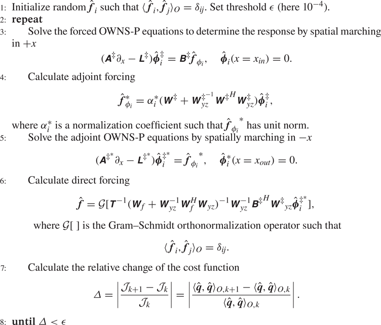

Figure 2. Schematic of the iterative adjoint-looping algorithm for the calculation of the optimal responses and forcings using the OWNS-P framework. By marching the direct and adjoint OWNS-P, instead of solving the globally discretized equations, significant computational savings are achieved.
Algorithm 1 constitutes a power iteration scheme augmented with Gram–Schmidt orthogonalization to allow computation of multiple modes. More sophisticated iteration schemes such as the Arnoldi method or RSVD (Halko, Martinsson & Tropp Reference Halko, Martinsson and Tropp2011) could be used to accelerate convergence. However, for the examples presented in § 5, we observed that the power iteration converges in just a few iterations. Accordingly, we have presented the power iteration scheme for the sake of simplicity and clarity.
In addition to finding optimal volumetric forcing and response modes, optimal initial (boundary) conditions, as previously done using PSE (Tempelmann, Hanifi & Henningson Reference Tempelmann, Hanifi and Henningson2010, Reference Tempelmann, Hanifi and Henningson2012), can be computed by restricting the input to the inlet plane, prolonging it to the solution space via  $\boldsymbol{\mathsf{B}}_q$ and, if desired, restricting the output to a smaller space, e.g. some downstream plane, via $\boldsymbol{\mathsf{C}}_q$.
5. Examples
In this section we present three example problems – a simple acoustics problem, a turbulent Mach 1.5 jet and a laminar Mach 4.5 boundary layer – to validate and demonstrate the OWNS-P method (§ 3) and its application for computing resolvent modes (§ 4). In each case, the OWNS-P results are validated against global calculations (§ 2) and, for the boundary layer, recent results from the literature (Bugeat et al. Reference Bugeat, Chassaing, Robinet and Sagaut2019).
5.1. Governing equations
The flow dynamics are governed by the compressible Navier–Stokes equations for an ideal gas,
 \begin{gather} \frac{D\rho}{D t} +\rho (\boldsymbol{\nabla} \boldsymbol{\cdot} \boldsymbol{u}) = 0, \end{gather}
 \begin{gather}\rho \frac{D \boldsymbol{u}}{D t} + \boldsymbol{\nabla} p = \frac{1}{Re} \boldsymbol{\nabla} \boldsymbol{\cdot} \tau, \end{gather}
 \begin{gather}\rho \gamma R \frac{DT}{D t} -(\gamma-1)\frac{Dp}{D t} = \frac{\gamma-1}{Pr Re}\boldsymbol{\nabla} \boldsymbol{\cdot} (k\boldsymbol{\nabla} T ) + \frac{\gamma-1}{Re} (\tau:\boldsymbol{\nabla} \boldsymbol{u}), \end{gather}
 \begin{gather}\tau = 2\mu S +\kappa (\boldsymbol{\nabla} \boldsymbol{\cdot} \boldsymbol{u})I, \end{gather}
 \begin{gather}S = \frac{1}{2}\left(\boldsymbol{\nabla} \boldsymbol{u} + (\boldsymbol{\nabla} \boldsymbol{u})^T - \frac{2}{3} (\boldsymbol{\nabla} \boldsymbol{\cdot} \boldsymbol{u})I\right), \end{gather}
 \begin{gather}p = \rho RT, \end{gather}
 \begin{gather}Re = \frac{\rho_\infty c_\infty L}{\mu_\infty}, \end{gather}
 \begin{gather}Pr = \frac{\mu_\infty{c_p}_\infty }{k_\infty}, \end{gather}
where  $\rho$, $\boldsymbol {u}$, $p$,
$p$,  $\gamma$, $R$,
$R$,  $T$,
$T$,  $k$,
$k$,  $\kappa$, $c$,
$c$,  $\mu$, $c_p$, $Re$ and $Pr$ are the density, velocity vector, pressure, specific heat ratio, gas constant, temperature, thermal conductivity, bulk viscosity, speed of sound, dynamic viscosity, isobaric specific heat, Reynolds number and Prandtl number, respectively (Kamal et al. Reference Kamal, Rigas, Lakebrink and Colonius2020). All relevant quantities have been non-dimensionalized by the dimensional ambient quantities $c_\infty$, $\rho _\infty$, $k_\infty$, ${c_p}_\infty$ and $\mu _\infty$, and a problem dependent length scale $L$.
$L$.
We define the state vector as  $q = (\rho, \boldsymbol {u}, T)^T$ and apply the Reynolds decomposition (2.2) to obtain the linearized equations (2.3). For some of the calculations, e.g. the acoustics problem, we employ a simplified formulation of the compressible Navier–Stokes equations described by Towne (Reference Towne2016).
We assume the fluid to be an ideal gas with  $c_v=c_v(T)$ and $c_p = c_p(T)$ and that fluid properties $k$,
$k$,  $\mu$, $\kappa$ and $\gamma$ depend solely on temperature. We denote any of the aforementioned fluid properties as $\varPhi$ and perform a Taylor series expansion about $\bar {T}$,
 \begin{equation} \varPhi(T) = \varPhi(\bar{T}) + \left.\frac{{\rm d} \varPhi}{{\rm d}T}\right|_{T=\bar{T}}T'+ \text{higher-order terms} . \end{equation}
The linearized fluid property perturbation is thus
 \begin{equation} \varPhi' = \left.\frac{{\rm d} \varPhi}{{\rm d}T}\right|_{T=\bar{T}}T'. \end{equation}
Unless otherwise stated, we will assume the fluid as calorically perfect air with  $\gamma =1.4$ and $Pr=0.72$ with viscosity and thermal conductivity calculated using Sutherland's law
 \begin{equation} \mu^{\dagger}{=} \mu^{\dagger}_\infty \left(\frac{T^{\dagger}}{T^{\dagger}_\infty} \right)^{3/2} \frac{T^{\dagger}_\infty + S^{\dagger}}{T^{\dagger}{+} S^{\dagger}},\end{equation}
where  $S^{\dagger} =110.4$ K and $()^{\dagger}$ denotes dimensional quantities.
The acoustics problem and the flat-plate boundary layer flow are solved in Cartesian coordinates with  $\boldsymbol {x} = (x,y,z)$ corresponding to the streamwise, wall-normal and spanwise directions, respectively, and $\boldsymbol {u}=(u, v, w)$. The jet flow is solved in cylindrical coordinates with $\boldsymbol {x} = (x,r,\theta )$ corresponding to the streamwise, radial and azimuthal directions, respectively, and $\boldsymbol {u}=(u_x, u_r, u_\theta )$. Due to the periodicity of the examined flows in the spanwise or azimuthal directions, the perturbation fields are decomposed as $\boldsymbol {q}' = \sum {\hat {\boldsymbol {q}}}(x,y) \exp (i \beta z - i \omega t)$ and $\boldsymbol {q}' = \sum {\hat {\boldsymbol {q}}}(x,r) \exp (i m \theta - i \omega t)$, where $\beta$ and $m$ are the spanwise and azimuthal wavenumbers, respectively.
All inner products, e.g.  $\langle \boldsymbol {a},\boldsymbol {b} \rangle _g$, are defined so as to induce the Chu energy norm (Chu Reference Chu1965)
 \begin{equation} E_{Chu} = \frac{1}{2}\int \int_\varOmega \frac{R \bar{T}}{ \bar{\rho}} \rho'^2 + \bar{\rho} |\boldsymbol{u'}|^2 + \frac{R \bar{\rho}}{\bar{T} (\gamma-1) }T'^2 \,{\rm d}x \,{\rm d}A \approx \int_\varOmega \boldsymbol{q}'^*\boldsymbol{\mathsf{W}}_{yz} \boldsymbol{\mathsf{W}}_e \boldsymbol{q}'\,{\rm d}x, \end{equation}
where  $\boldsymbol{\mathsf{W}}_e$ is the diagonal Chu energy weight matrix defined as
 \begin{equation} \boldsymbol{\mathsf{W}}_e = \frac{1}{2}\begin{bmatrix} \dfrac{R \bar{T}}{ \bar{\rho}} & 0 & 0 & 0 & 0 \\ 0 & \bar{\rho} & 0 & 0 & 0 \\ 0 & 0 & \bar{\rho} & 0 & 0 \\ 0 & 0 & 0 & \bar{\rho} & 0 \\ 0 & 0 & 0 & 0 & \dfrac{R \bar{\rho}}{\bar{T}(\gamma-1) }\end{bmatrix}. \end{equation}
5.2. Global and OWNS solvers
The global and OWNS calculations are performed using the Caltech stability and transition analysis toolkit. The linearized equations are discretized in inhomogeneous transverse directions using fourth-order central finite differences with summation-by-parts boundary closure (Strand Reference Strand1994; Mattsson & Nordstróm Reference Mattsson and Nordstróm2004). Far-field radiation boundary conditions are enforced at free transverse boundaries using a super-grid damping layer (Appelo & Colonius Reference Appelo and Colonius2009) truncated by Thompson characteristic conditions (Thompson Reference Thompson1987). For global calculations, the streamwise direction is discretized using the same scheme and streamwise boundary conditions are implemented using inlet and outlet sponges in addition to the characteristic boundary conditions. For OWNS calculations, the numerical treatment of the  $x$ direction is slightly different in each problem and is reported in the following subsections. Additional details of the code can be found in Kamal et al. (Reference Kamal, Rigas, Lakebrink and Colonius2021).
An important consideration in the calculation of the OWNS response is the placement of the recursion parameters. For all cases, we follow the general recipe presented by Towne & Colonius (Reference Towne and Colonius2015). An estimate for the eigenvalues of the downstream and upstream modes for each frequency and for each streamwise location can be obtained assuming locally parallel and uniform flow equal to the free-stream velocity. The effectiveness of the OWNS-P projection to accurately filter the upstream-travelling modes without modifying the downstream ones is demonstrated in figure 3, where the local (in  $x$) spectra of the Navier–Stokes and OWNS-P equations are shown for the boundary layer problem discussed in § 5.5 for three values of $N_{\beta }$. The spectra were calculated by solving a generalized eigenvalue problem obtained from the unforced (homogeneous) form of (3.46) by assuming a locally parallel flow, for which $\partial _x \to i \alpha$ and the complex streamwise wavenumber $\alpha$ is the eigenvalue.

Figure 3. Placement of recursion parameters  $\beta ^+$ and $\beta ^-$ for the $M=4.5$ flat-plate boundary layer flow. The local spectra of the Navier–Stokes and OWNS-P operators are shown. The $\beta ^+$ recursion parameters are placed near the downstream-travelling modes, whereas the $\beta ^-$ parameters are placed near the upstream acoustic modes. For a sufficiently large number $N_\beta$ of recursion parameters, the OWNS-P operator converges to the downstream-travelling modes, thus eliminating the ellipticity associated with upstream modes and enabling stable, convergent marching in the slowly varying $x$ direction.
5.3. Dipole forcing of a quiescent fluid
In this problem a 2-D dipole forcing is used to excite waves in an inviscid quiescent fluid. The right-hand-side forcing that is applied to the energy equation is shown in figure 4(a), and the proper forcing terms are applied to the other equations in order to produce a dipole response in the pressure field, which is shown in figure 4(d). This is an exact solution of the Euler equations.

Figure 4. Dipole test case: (a) forcing applied to the energy equation; (b) OWNS-P downstream-travelling pressure response; (c) OWNS-P upstream-travelling pressure response; (d) exact pressure response; (e) OWNS-P total pressure response recovered by summing the downstream- and upstream-travelling solutions; (f) error computed as the difference between the total OWNS-P and exact pressure responses, normalized by the maximum of the exact pressure.
We use the OWNS-P method to obtain an approximate solution. The computational domain extends ten wavelengths in both  $x$ and $y$ and is discretized using $200$ equally spaced points in each direction. No incoming fluctuations are specified at the domain boundaries – the waves are excited exclusively by the inhomogeneous forcing terms.
The pressure field obtained by integrating the one-way equations from left to right is shown in figure 4(b). Clearly, the downstream-travelling waves are accurately captured. Similarly, the pressure field obtained by integrating from right to left is shown in figure 4(c). This time, the upstream-travelling waves are captured. Since the governing equations are  $x$-independent in this problem, the full solution can be recovered by summing the downstream- and upstream-travelling solutions, which is shown in figure 4(e). The error in the full OWNS-P solution, relative to the exact solution, is shown in figure 4(f). The total $L_2$ error is $0.28\,\%$, and this error is concentrated at angles nearly perpendicular to the marching direction as measured from the position of the source. As shown by Towne & Colonius (Reference Towne and Colonius2015), these high angles converge with $N_{\beta }$ at a slower, but still exponential, rate than lower angles.
5.4. Supersonic turbulent jet
Next, we demonstrate our method using the example of a turbulent jet. Resolvent analysis has been applied to jets by numerous authors (Garnaud et al. Reference Garnaud, Lesshafft, Schmid and Huerre2013; Jeun et al. Reference Jeun, Nichols and Jovanović2016; Schmidt et al. Reference Schmidt, Towne, Rigas, Colonius and Brès2018; Lesshafft et al. Reference Lesshafft, Semeraro, Jaunet, Cavalieri and Jordan2019), and resolvent modes have been shown to capture a rich set of physical phenomena. These include the Kelvin–Helmholtz instability, which leads to large-scale coherent wavepacket structures (Jordan & Colonius Reference Jordan and Colonius2013), the Orr mechanism (Tissot et al. Reference Tissot, Zhang, Lajús, Cavalieri and Jordan2017; Schmidt et al. Reference Schmidt, Towne, Rigas, Colonius and Brès2018), the lift-up mechanism (Nogueira et al. Reference Nogueira, Cavalieri, Jordan and Jaunet2019; Pickering et al. Reference Pickering, Rigas, Nogueira, Cavalieri, Schmidt and Colonius2020) and trapped acoustic waves within the jet core (Tam & Hu Reference Tam and Hu1989; Towne et al. Reference Towne, Cavalieri, Jordan, Colonius, Schmidt, Jaunet and Brès2017b). The slow spread of the jet makes OWNS applicable, and the diverse set of physics embedded within the resolvent operator make it a challenging test case.
We will make comparisons between a standard global solution of the linearized Navier–Stokes equation and those obtained using OWNS-P (and OWNS-O and PSE when applicable). The global solution comprises the result of applying the resolvent operator to a given forcing vector, giving a point of comparison for the approximation of this action provided by the OWNS-P method.
We consider the specific case of a jet with Mach number  $M = U_{j} / c_{\infty } = 1.5$, Reynolds number $Re = \rho _{j} U_{j} D / \mu = 1760 000$ and temperature ratio $T_{j}/T_{\infty } = 1$, where the subscripts $j$ and $\infty$ denote conditions at the jet nozzle exit and in the far field, respectively. The mean flow about which the Navier–Stokes equations are linearized is obtained from a large-eddy simulation (LES) described by Brès et al. (Reference Brès, Ham, Nichols and Lele2017) and is shown in figure 5. Within the linearized equation, we use a turbulent Reynolds number of $Re_T = 1760$, three orders of magnitude less than the true Reynolds number. This choice is motivated by recent work showing that using an eddy-viscosity model or reduced effective Reynolds number improves both the near-field (Pickering et al. Reference Pickering, Rigas, Schmidt, Sipp and Colonius2021a) and far-field (Pickering et al. Reference Pickering, Towne, Jordan and Colonius2021b) predictions in free-shear flows.

Figure 5. Mean flow of the  $M=1.5$ turbulent jet. Local Mach number is shown.
The linearized equations in cylindrical coordinates are discretized in the radial direction as described earlier, and boundary conditions at the polar axis are enforced using the approach of Mohseni, Colonius & Freund (Reference Mohseni, Colonius and Freund2002). The physical portion of the domain extends to  $r/D = 6$ and is discretized using 150 grid points with a higher concentration around the shear layer at $r/D = 0.5$, while the damping layer contains an additional 50 points. While the LES from which the mean flow is obtained includes the nozzle within the computational domain, the resolvent calculations do not; previous publications have shown that excluding the nozzle does not hinder favourable comparisons with data (Schmidt et al. Reference Schmidt, Towne, Rigas, Colonius and Brès2018; Pickering et al. Reference Pickering, Rigas, Nogueira, Cavalieri, Schmidt and Colonius2020). Since the mean flow is axisymmetric, the azimuthal direction is homogeneous and can be decomposed into a Fourier series. In what follows, we focus on the axisymmetric mode ( $m=0$), which is often of foremost interest in the study of jet aeroacoustics (Cavalieri et al. Reference Cavalieri, Jordan, Colonius and Gervais2012; Chen & Towne Reference Chen and Towne2021).
The streamwise grid for each method extends from  $x/D = 0.5$ to 30 with equidistant spacing of ${\rm \Delta} x = 0.05$ (with the exception of the PSE method, which determines its own step size) and an additional sponge region included in the global computation at three diameters upstream and downstream. The OWNS-O and OWNS-P equations are integrated in the streamwise direction using the second-order backward difference formula and a fifth-order Runge–Kutta Radau II scheme, respectively (Hairer & Wanner Reference Hairer and Wanner1971). Here $N_{\beta } = 13$ recursion parameters are used for estimating the OWNS operators. In the following subsections, we show results for two frequencies, $St = 0.26$ and 0.52, which are close to the frequency of maximum acoustic radiation (Jordan & Colonius Reference Jordan and Colonius2013) and maximum near-field resolvent gain (Schmidt et al. Reference Schmidt, Towne, Rigas, Colonius and Brès2018), respectively.
5.4.1. Near-nozzle Kelvin–Helmholtz forcing
First, we compute the downstream response of the linearized equations to a disturbance near the nozzle exit, and compare the OWNS-P solution to those obtained using PSE, OWNS-O and a global computation. Specifically, the local Kelvin–Helmholtz eigenfunction is specified at  $x/D = 0.5$ as an initial condition in the PSE and OWNS marches and as a boundary condition for the global method. The solution can be interpreted as the response to a localized forcing at the upstream boundary. In other words, we are computing the result of applying the resolvent operator, approximated by each method, to a forcing vector that is localized at the upstream boundary and which specifically excites the Kelvin–Helmholtz instability.
Results of this test case are shown in figure 6, which shows the pressure field computed by each method for  $St = 0.26$ and 0.52. The OWNS-P solution closely matches the global solution for both frequencies, demonstrating that the OWNS-P method provides a good approximation of the action of the resolvent operator on the Kelvin–Helmholtz forcing vector. The OWNS-P solution also matches the OWNS-O solution, which has been previously validated for a similar turbulent jet (Towne & Colonius Reference Towne and Colonius2015). As shown by Sinha et al. (Reference Sinha, Rodriguez, Bres and Colonius2014) and others, PSE also provides a reasonable solution for supersonic jets forced by a Kelvin–Helmholtz mode. In this case PSE performs well because its underlying assumptions are valid; we have artificially excited a single instability mode by using the Kelvin–Helmholtz mode as an initial condition. While the acoustic radiation is slightly damped compared with the other three solutions, especially for $St = 0.26$, it is also reasonably captured because its wavelength is nearly the same as the Kelvin–Helmholtz mode for low-supersonic jets (Towne et al. Reference Towne, Rigas and Colonius2019). However, PSE cannot handle more complex forcings such as those considered next.

Figure 6. Response of the jet to the Kelvin–Helmholtz initial condition at  $x/D = 0.5$ using global, PSE, OWNS-O and OWNS-P methods, top to bottom, respectively. Contours of pressure are shown in each panel.
5.4.2. Volumetric forcing using LES data
Second, we use both OWNS-P and the standard global approach to compute the response of the linearized equations to global forcing vectors extracted from LES data. The right-hand-side forcing term  $\boldsymbol {f}$ in (2.3) is obtained by computing the two left-hand-side terms using the LES approximation of the nonlinear Navier–Stokes operator $\mathcal {N}$. The first term can be computed as
 \begin{equation} \frac{\partial q'}{\partial t} = \frac{\partial q}{\partial t} = \mathcal{N}(q), \end{equation}
since  $\bar {q}$ does not depend on time (Towne Reference Towne2016). The second term can be approximated as
 \begin{equation} \mathcal{A}(\bar{q}) q' = \frac{\partial \mathcal{N}}{\partial q} (\bar{q})q' \approx \frac{\mathcal{N}(\bar{q}+\epsilon q') - \mathcal{N}(\bar{q})}{\epsilon} \end{equation}
for some  $\epsilon \ll 1$ (de Pando, Sipp & Schmid Reference de Pando, Sipp and Schmid2012). We take $\epsilon = 10^{-7}$ and note that the results are nearly independent of $\epsilon$ over a range spanning at least four orders of magnitude. Details of the procedure can be found in Towne (Reference Towne2016).
After performing an azimuthal Fourier transform, an ensemble of realizations of  $\boldsymbol {\hat {q}}$ and $\boldsymbol {\hat {f}}$ are obtained from the LES data by segmenting $\boldsymbol {q}^{\prime }$ and $\boldsymbol {f}$ into overlapping blocks, each containing $N_{f}$ snapshots of data. We use blocks of length $N_{f} = 256$ with 80 % overlap and employ the $w_{C_{4}^{\infty }}$ window proposed by Martini et al. (Reference Martini, Cavalieri, Jordan and Lesshafft2019) to minimize spectral leakage. This results in 189 realizations of the flow at discrete frequencies, separated by ${\rm \Delta} St = 0.02604$.
Each of these  $\boldsymbol {\hat {q}}$, $\boldsymbol {\hat {f}}$ pairs approximately satisfy (2.6). That is, applying the resolvent operator to $\boldsymbol {\hat {f}}$ yields $\boldsymbol {\hat {q}}$. This relationship is approximate for the LES data for two reasons. First, by necessity, we used a finite length discrete Fourier transform in place of an infinite and continuous Fourier transform to obtain $\boldsymbol {\hat {q}}$ and $\boldsymbol {\hat {f}}$, leading to aliasing and spectral leakage. In particular, $\boldsymbol {\hat {q}}$ exhibits a relatively flat spectrum up to moderate frequencies, making it especially susceptible to aliasing (Towne, Brès & Lele Reference Towne, Brès and Lele2017a; Karban et al. Reference Karban, Martini, Jordan, Brès and Towne2022). Second, the forcing term $\boldsymbol {f}$ was defined implicitly using the LES operator as described above, whereas our resolvent operator is obtained by explicitly linearizing the Navier–Stokes equations and discretizing the linear equations using numerics different from those within the LES. Thus, we do not expect our global and OWNS-P approximation of the action of the resolvent operator on $\boldsymbol {\hat {f}}$ to exactly reproduce the corresponding $\boldsymbol {\hat {q}}$ obtained from the LES data. Nevertheless, the $\boldsymbol {\hat {f}}$ vectors obtained from the LES data provide a physically motivated forcing that can be used to compare the action of the resolvent operators obtained via the OWNS-P march and the standard global solution.
Figure 7 shows one realization of the forcing and response for  $St = 0.26$ and 0.52. Specifically, we show the component of the forcing that is applied to the energy equation and the response of the pressure field; other components of the forcing and response are qualitatively similar (Towne Reference Towne2016). The forcing is rather incoherent and lacks readily visible large-scale structures. In contrast, the pressure field contains distinct wavepacket structures and an acoustic beam emanating from the near field to the far field. Despite the lack of structure within the forcing, its introduction as a volumetric forcing term to the global and OWNS-P operators produces a response that is quite similar to the LES pressure field. Some minor differences can be observed, e.g. both the global and OWNS-P solutions contain stronger acoustic waves downstream of the main beam near the top-right corner of the figure. These and other minor differences can be attributed to the factors described earlier.

Figure 7. Realizations of the Mach 1.5 jet, including an LES-derived forcing and pressure response realization (top two rows, respectively) and global and OWNS-P computed pressure realizations (bottom two rows, respectively) forced with the above LES forcing realization.
Of greater relevance to the current study, the OWNS-P response closely matches the global response. For both frequencies, the OWNS-P response accurately captures the relevant dynamics in the jet, including near-field structures such as Kelvin–Helmholtz wavepackets (similar to those observed in figure 3) and Orr-type wavepackets (farther downstream, e.g.  $15< x/D,20$), as well as the angle and intensity of acoustic radiation to the far field. This substantial agreement between the global and OWNS-P responses indicates that the OWNS-P approximation of the action of the resolvent operator on this forcing vector accurately mimics that of the global resolvent operator.
The ensemble of LES flow and forcing realizations can be used to compute the average error of the OWNS-P approximation over many potential forcing vectors. Figure 8 shows the power spectral density (PSD) of the LES, global and OWNS-P pressure fields for  $St = 0.26$ and 0.52, i.e. the squared amplitude of the response averaged over the ensemble of realizations. In each case, the PSD is scaled by the maximum value of the PSD of the LES data. The PSD of the global and OWNS-P solutions accurately mimic that of the LES data. More importantly, the PSD computed from the ensemble of OWNS-P solutions closely matches the PSD computed from the global solutions. Both the envelope of the high-energy near-field region and intensity and directivity of the acoustic beam show good agreement for both frequencies.

Figure 8. Full-field pressure PSD results for LES (a,b), global (c,d) and OWNS-P (e,f).
A more quantitative assessment is provided in figure 9, which shows the PSD of the LES, global and OWNS-P pressure fields as a function of  $x/D$ at $r/D = 0.5$ (the jet lip line) and $r/D = 6$ (the maximum radial position of the physical domain). The OWNS-P solution closely matches the global solution except in two low-energy regions where upstream-travelling waves are non-negligible. First, OWNS-P undershoots the global solution very close to the nozzle for $r/D=0.5$. Since the solution was initiated with a zero boundary condition, the downstream-travelling waves have not yet developed at the nozzle inlet, allowing the weak influence of upstream-travelling waves to be observed. Second, the global solution contains weak upstream-travelling acoustic waves that cannot be captured via one-way marching, resulting in an under prediction by OWNS-P along $r/D=6$ for $x/D<5$, well away from the main acoustic beam observed at higher values of $x/D$. Both of these minor discrepancies are expected given the one-way nature of OWNS.

Figure 9. Pressure PSD for LES (blue), global (orange) and OWNS-P (yellow) for (a)  $St = 0.26$; (b) $St = 0.52$. Solid and dashed lines correspond to $r/D = 0.5$ and 6, respectively.
The PSD of the error between the global and OWNS-P solutions, normalized by the maximum value of the PSD of the global solution, is shown in figure 10. Comparing with figure 8, the average error is observed to be at least an order of magnitude smaller than the average solution in both the near-field hydrodynamic region and the acoustic field. Overall, these results indicate that the OWNS-P method provides an accurate approximation of the action of the resolvent operator for the ensemble of forcing realizations extracted from the LES data. Physically, the accuracy of the OWNS-P solution confirms the dominance of downstream-travelling waves in the forced jet.

Figure 10. Full-field error between global and OWNS-P pressure PSD.
5.4.3. Optimal forcing and response
Next, we show that the OWNS-P framework provides an accurate approximation of the global optimal forcing and response modes. The input forcing has been constrained to  $0.5 < x/D < 30$, $R_{min} < r/D < R_{max}$. We use $R_{min}=0.0425$ to prevent the forcing from damaging the pole conditions (Mohseni et al. Reference Mohseni, Colonius and Freund2002) and $R_{max}$ is defined as the radial jet location where the velocity is greater than $5\,\%$ of the maximum jet velocity, i.e. the forcing is contained only within the jet. The output is defined in the full numerical domain, $0.5 < x/D < 30, 0 < r/D < 17$.
The real part of the optimal pressure forcing and response from the OWNS-P and global resolvent methods for  $St=0.26$ and $0.52$ and $m=0$ are shown in figure 11. At these frequencies, the response is dominated by the amplification of disturbances due to the Kelvin–Helmholtz instability (Schmidt et al. Reference Schmidt, Towne, Rigas, Colonius and Brès2018; Pickering et al. Reference Pickering, Rigas, Nogueira, Cavalieri, Schmidt and Colonius2020). The global and OWNS-P solutions are shown along the jet lip line $r/D=0.5$ in figure 12. Quantitative agreement is obtained, justifying the assumption of weak influence of the upstream-travelling modes during the OWNS-P parabolization procedure.

Figure 11. Optimal forcing (a–d) and response (e–h) for the  $M=1.5$ turbulent jet. Comparison between global (a,b,e,f) and OWNS-P (c,d,g,h). Contours of the real pressure component at $St=0.26$ and $St=0.52$ are shown.

Figure 12. Optimal pressure response for the jet along  $r/D = 0.5$ for (a) $St = 0.26$ and (b) $St = 0.52$. Solid and dashed lines show the global and OWNS-P solutions, respectively.
5.5. Mach 4.5 boundary layer
Finally, we consider a Mach 4.5 laminar flat-plate zero-pressure-gradient boundary layer. Optimal forcing and response modes are computed using the OWNS-P and global methods for several frequency and wavenumber combinations corresponding to different instability mechanisms. These cases, and the numerical parameters used for each, are summarized in table 1.
Table 1. Numerical parameters for the supersonic boundary layer cases.

All boundary layer quantities are non-dimensionalized using the free-stream velocity  $U_{\infty }$ and the local compressible displacement thickness $\delta ^*(x)$ or the displacement thickness at the outlet of the domain $\delta ^*_0$. The Mach number is $M=U_{\infty } / c_{\infty }=4.5$. The outlet of the domain is at $Re_x^{out} = {\nu _\infty x}/{U_{\infty }} = 1.74\times 10^6$, or $Re_{\delta ^*_0}^{out}=11,216$. The domain inlet is located a small distance form the leading edge at $Re_x^{in} = 105$, corresponding to ${Re_{\delta ^*_0}^{in}=871}$, to avoid the singularity in the similarity solution that we use in this study. The domain size is similar to that of Bugeat et al. (Reference Bugeat, Chassaing, Robinet and Sagaut2019), where in their calculations the outlet is at $Re_x^{out} = 1.75\times 10^6$ or $Re_{\delta ^*_0}^{out}=11 000$. However, in their calculations the flat-plate leading edge was also included in the computational domain, resulting in a weak shock at the leading edge and small discrepancies in the momentum thickness at the outlet compared with the similarity solution.
In order to properly resolve the instabilities near the wall and critical layer, grid stretching in the  $y$ direction is employed clustering half of the points near the wall for $y/{\delta ^*_0}<0.9$ (Malik Reference Malik1990). No-slip and adiabatic boundary conditions ( $\hat {u}=\hat {v}=\hat {w}=\partial \hat {T} / \partial y =0$) are enforced at the wall (Poinsot & Lele Reference Poinsot and Lele1992). Integration of the OWNS-P equations in $x$ is performed using a second-order backward differentiation formula. As indicated in table 1, fewer $x$ grid points were used for the global calculation due to the higher-order discretization and computational limitations due to its large memory requirements.
All calculations were performed with  $N_{\beta }=15$, which gave a good approximation for the filtering of the upstream-travelling modes and accurate capturing of the downstream ones.
5.5.1. Base flow
The laminar base flow is obtained from a similarity solution of the compressible boundary layer equations. The Howarth–Dorodnitsyn transformation (Stewartson Reference Stewartson1964) was employed to reduce the governing equations to a set of ODEs, given in Appendix D. The similarity solution is shown in figure 13.

Figure 13. Base flow of the  $M=4.5$ adiabatic flat-plate boundary layer obtained from a similarity transformation. Self-similar streamwise and temperature components (a). Local Mach number (b) with the dashed line corresponding to the displacement thickness.
5.5.2. Optimal gain
The resolvent modes for the adiabatic flat-plate boundary layer have been calculated with the optimal OWNS-P method for a range of frequencies and spanwise wavenumbers. In figure 14 the optimal input/output gains corresponding to three regions of locally maximum gain in the  $\beta \unicode{x2013}\omega$ plane are shown. Their maxima correspond to the amplification of streaks ( $\omega \to 0$), second Mack modes ( $\beta =0$) and oblique first modes. For all three instability types, we observe excellent agreement of the optimal $\omega$ and/or $\beta$ when compared with the global resolvent calculations of Bugeat et al. (Reference Bugeat, Chassaing, Robinet and Sagaut2019). For all the calculations presented here, the forcing has been restricted only to the momentum components $(f_u,f_v,f_w)$ to match the set-up of Bugeat et al. (Reference Bugeat, Chassaing, Robinet and Sagaut2019).

Figure 14. Optimal input/output gain for three linear instability mechanisms for the  $M=4.5$ flat-plate adiabatic boundary layer. Validation against normalized results from Bugeat et al. (Reference Bugeat, Chassaing, Robinet and Sagaut2019) for a similar configuration.
5.5.3. Optimal forcing and response
For streaks, the optimal forcing consists of streamwise counter-rotating vortices that lift the streamwise base flow momentum. This is referred to as the lift-up mechanism and yields a response that contains primarily streaks of highly amplified streamwise velocity stretching in the streamwise direction. The dominant input ( $f_v$) and output ( $\hat {u}$) velocity modes from OWNS-P and global methods are shown in figure 15. Quantitative agreement is again obtained between the OWNS-P optimal modes and the global ones, but minor differences are observed near the inlet/outlet boundaries of the domain, where the sponges of the global method attenuate the response to avoid reflections. Based on our experience, the tuning of the sponges is a cumbersome procedure and problem specific, a step that is bypassed during the OWNS-P marching since upstream-travelling waves have been eliminated at each $x$ location during the parabolization procedure.

Figure 15. Streak (steady 3-D) optimal disturbances at  $\omega =0.002$, $\beta =2.2$. Forcing and response amplitude components at $x/\delta ^*_0=35$ (a,c,e) and $x/\delta ^*_0=159$ (b,d,f). Circle symbols: Bugeat et al. (Reference Bugeat, Chassaing, Robinet and Sagaut2019); triangle symbols: global; solid lines: OWNS-P.
In figure 15 we also plot the OWNS-P optimal forcing and response profiles for all the perturbation components at a fixed streamwise location near the inlet and outlet, respectively. The OWNS-P results are compared against our global calculations for the same configuration and the global calculations from Bugeat et al. (Reference Bugeat, Chassaing, Robinet and Sagaut2019). Quantitative agreement is again obtained between OWNS-P and our global results, confirming the accuracy of the OWNS-P approximation. Some discrepancies are observed for the forcing away from the wall when our results (both global and OWNS-P) are compared against Bugeat et al. (Reference Bugeat, Chassaing, Robinet and Sagaut2019). These discrepancies can be attributed to the differences in the computational domain (inclusion of leading edge and shock) and the different choice of the input norm between the two studies. The forcing amplitudes presented in Bugeat et al. (Reference Bugeat, Chassaing, Robinet and Sagaut2019) likely correspond to the conservative form of the momentum equations, whereas we perform our analyses using primitive variables (Karban et al. Reference Karban, Bugeat, Martini, Towne, Cavalieri, Lesshafft, Agarwal, Jordan and Colonius2020). Essentially, our forcing exists in a different subspace, but we are optimizing the same quantity, i.e. the disturbance-energy amplification with respect to the Chu energy norm, which explains the agreement observed in the response profiles despite the differences in the forcing modes.
Contours of the optimal forcing and response for the oblique first mode are shown in figure 16 for the dominant components  $f_w$ and $\hat {u}$ from the OWNS-P and global calculations. The optimal forcing field contains upstream-titled structures that are emblematic of the non-modal Orr mechanism. This generates an oblique wave response with relatively large streamwise velocity. Good agreement is obtained between the global and OWNS-P results for all the perturbation input and output components, although a small error of about $1\,\%$ in the wavelength can be observed.

Figure 16. Oblique first mode (unsteady 3-D) optimal disturbances at  $\omega =0.32$, $\beta =1.2$. Forcing and response amplitude components at $x/\delta ^*_0=12$ (a,c,e) and $x/\delta ^*_0=159$ (b,d,f). Circle symbols: Bugeat et al. (Reference Bugeat, Chassaing, Robinet and Sagaut2019); triangle symbols: global; solid lines: OWNS-P.
In figure 17 we compare the results for the second mode instability, following a similar procedure as in the two previous cases. We see the classical trapped acoustic waves between the wall and relative sonic line as well as thermodynamic amplification near the generalized inflection point in the response fields (two coexisting mechanisms). For such a response, the optimal forcing is localized near the generalized inflection point. Good agreement is also obtained between OWNS-P and our global results for this family of modes.

Figure 17. Planar second mode (unsteady 2-D) optimal disturbances at  $\omega =2.5$, $\beta =0$. Forcing and response amplitude components at $x/\delta ^*_0=90$ (a,c,e) and $x/\delta ^*_0=148$ (b,d,f). Circle symbols: Bugeat et al. (Reference Bugeat, Chassaing, Robinet and Sagaut2019); triangle symbols: global; solid lines: OWNS-P.
The close agreement between the global and OWNS-P modes extends also to suboptimal modes. For example, figure 18 compares the global and OWNS-P streamwise velocity response for the first suboptimal modes, i.e. the mode with the second highest gain, for each of the three instability mechanisms.

Figure 18. Streamwise velocity response for the first suboptimal mode computed by the global and OWNS-P methods: (a,b) streaks; (c,d) oblique first mode; (e,f) planar second mode.
6. Conclusions
Computing resolvent modes for flows with multiple inhomogeneous directions remains a computationally intensive task. In this paper we have developed a new method that reduces the cost of computing resolvent modes for flows that include a slowly varying direction.
Our computationally efficient approach contains two parts. First, we showed how the action of the resolvent operator on a forcing vector can be accurately approximated using a spatial marching method. This constitutes an extension of the OWNS methodology introduced by Towne & Colonius (Reference Towne and Colonius2015) to accommodate a forcing term on the linear equations, which is central to the concept of resolvent analysis. The method is based on an approximation of the projection operator that rigorously splits the solution vector into downstream- and upstream-travelling components. Applying this projection operator to the linearized Navier–Stokes equations yields a well-posed equation governing the downstream evolution of the flow, which can be stably integrated in the slowly varying direction. By construction, the influence of upstream-travelling waves on downstream-travelling waves is neglected in the one-way march. This projection-based method, which we call OWNS-P, uses the same recursion parameters and inherits the same convergence properties as the previous outflow-based OWNS methodology, OWNS-O, of Towne & Colonius (Reference Towne and Colonius2015). Unlike the ubiquitous PSE, the OWNS-P method is capable of capturing the complete downstream response of the flow rather than a single instability mechanism (Towne et al. Reference Towne, Rigas and Colonius2019).
Second, we leverage the ability of OWNS-P to efficiently and accurately approximate the action of the resolvent operator to compute global resolvent modes at substantially reduced cost. Using an adjoint-based optimization framework, volumetric forcings that optimally excite and reveal the dominant 3-D instabilities of the flow are computed by marching the forward and adjoint OWNS-P equations in the downstream and upstream directions, respectively. Thus, we bypass the solution of direct and adjoint globally discretized Navier–Stokes equations, which can be computationally expensive or even intractable for 3-D inhomogeneous (base) flows.
This one-way marching methodology relies on the convective nature of fluid flow and, in particular, on the dominance of convective modal and non-modal instability mechanisms in slowly varying shear flows (Huerre & Monkewitz Reference Huerre and Monkewitz1990; Schmid & Henningson Reference Schmid and Henningson2001). This limits the applicability of our approach to globally stable flows, the same class of flows to which resolvent analysis is most naturally applied.
The OWNS-P method was demonstrated using three problems: a simple acoustics problem, a turbulent Mach 1.5 jet and a laminar Mach 4.5 boundary layer. For the jet, we showed that the OWNS-P solution faithfully approximates the action of the resolvent operator on both a localized forcing near the nozzle exit designed to excite the Kelvin–Helmholtz instability and a distributed volumetric forcing extracted from LES data. In the latter case, the OWNS-P solution captured all three prominent downstream-travelling mechanisms present in the jet: Kelvin–Helmholtz, Orr and acoustic waves. Consequently, the optimal forcing and response modes were accurately computed using the iterative marching technique. Similarly, for the boundary layer, we showed that the optimal OWNS-P methodology faithfully computed the gains and forcing and response modes associated with several different instability mechanisms, including streaks, the second Mack mode and oblique modes. In both cases, the OWNS-P framework was validated against global modes calculated by discretizing in all inhomogeneous spatial directions.
The close agreement between the ONWS-P and global methods strongly implies that the considered flows lack any significant (in terms of amplification) acoustic feedback mechanisms or other upstream-travelling waves. While previous work using parallel-flow stability theory and PSE are predicated on this result, neither framework captures the full spectrum of downstream-travelling modes, leaving room for doubt that is eliminated by the present approach. Apart from the computational advantages, the examples also show that OWNS-P provides a bridge between global amplification mechanisms, which are often difficult to interpret, and those from classical local spatial instability approaches, for which the physics underlying various modes are often well understood (Schmid & Henningson Reference Schmid and Henningson2001). For example, the OWNS-P solution at any streamwise position can be readily projected onto the associated parallel-flow eigenspectrum to reveal the local contribution of each downstream-travelling mode.
In the future, we believe that OWNS-P will enable computation of global resolvent modes that reveal the dominant instability mechanisms within previously intractable 3-D flows that contain a slowly varying direction, including swept wings and other 3-D aerodynamic bodies and jets with non-circular nozzles, e.g. rectangular jets and other complex nozzle geometries typical of modern tactical aircraft.
The OWNS methodology is also applicable to other problems beyond computation of resolvent modes. For example, OWNS could be used to find the downstream receptivity to an incident disturbance, compute kernels for closed-loop flow control or predict flow statistics based on stochastic forcing. Indeed, any problem to which PSE can be applied can also be addressed using OWNS, and the latter approach will provide greater accuracy for problems containing multiple relevant physical mechanisms, e.g. multiple instability modes, transient growth or acoustics. The proper choice between the original OWNS-O method and the OWNS-P method developed in this paper is dictated by the need, or lack-there-of, for a forcing term: only the OWNS-P method can accommodate a forcing term, but at the cost of solving a system of recursion equations that is twice as large compared with the OWNS-O approach.
Furthermore, the OWNS-P framework can be used for the calculation of nonlinear optimal disturbances (Rigas, Sipp & Colonius Reference Rigas, Sipp and Colonius2021) by including a finite number of harmonic balanced nonlinear interactions in the Lagrangian formulation. Calculation of nonlinear disturbances in compressible regimes has been attempted in the past using nonlinear PSE, which cannot account for multimodal instabilities or non-normal amplification mechanisms (Towne et al. Reference Towne, Rigas and Colonius2019), which play a key role during the transition process.
Acknowledgements
The authors thank Mr. L. Heidt for his assistance in analysing and measuring the FLOPS and memory requirements reported in § 3.6.
Funding
A.T. was supported in part by a catalyst grant from the Michigan Institute for Computational Discovery and Engineering (MICDE). G.R., O.K., E.P. and T.C. were supported by the Boeing Company through a Strategic Research and Development Relationship Agreement CT-BA-GTA-1 and by ONR grants N0014-11-1-0753, N00014-16-1-2445 and N00014-21-1-2158. O.K. also acknowledges support from the Natural Sciences and Engineering Research Council of Canada via the Postgraduate Doctoral Scholarship (PGSD3-532522-2019).
Declaration of interests
The authors report no conflict of interest.
Appendix A. Analytical solution of the recursion equations
In this appendix we provide an analytical solution of the recursion (3.40), which leads to the expression for  $\boldsymbol{\mathsf{P}}_{N_{\beta }}$ given in (3.42).
We begin by writing (3.40b)–(3.40d) in terms of the expansion coefficients  $\boldsymbol {\psi }^{j} = \boldsymbol{\mathsf{U}}\boldsymbol {\hat {\phi }}_{\pm }^{j}$,
 \begin{gather} (\boldsymbol{\mathsf{D}} - i \beta_{-}^{j} \boldsymbol{\mathsf{I}} ) \boldsymbol{\psi}^{{-}j} - (\boldsymbol{\mathsf{D}} - i \beta_{+}^{j} \boldsymbol{\mathsf{I}} ) \boldsymbol{\psi}^{{-}j-1} = 0 \quad j = 1,\ldots,N_{\beta}-1, \end{gather}
 \begin{gather}(\boldsymbol{\mathsf{D}} - i \beta_{-}^{0} \boldsymbol{\mathsf{I}} ) \boldsymbol{\psi}^{0} - (\boldsymbol{\mathsf{D}} - i \beta_{+}^{0} \boldsymbol{\mathsf{I}} ) \boldsymbol{\psi}^{{-}1} = (\boldsymbol{\mathsf{D}} - i \beta_{-}^{0} \boldsymbol{\mathsf{I}} ) \boldsymbol{\psi}, \end{gather}
 \begin{gather}(\boldsymbol{\mathsf{D}} - i \beta_{+}^{j} \boldsymbol{\mathsf{I}} ) \boldsymbol{\psi}^{j} - (\boldsymbol{\mathsf{D}} - i \beta_{-}^{j} \boldsymbol{\mathsf{I}} ) \boldsymbol{\psi}^{j+1} = 0 \quad j = 0,\ldots,N_{\beta}-1. \end{gather}
Since  $\boldsymbol{\mathsf{D}}$ is diagonal, each scalar component of $\boldsymbol {\psi }^{j}$ can be treated separately,
 \begin{gather} (i \alpha_{k} - i \beta_{-}^{j} \boldsymbol{\mathsf{I}} ) \boldsymbol{\psi}^{{-}j}_{k} - (i \alpha_{k} - i \beta_{+}^{j} \boldsymbol{\mathsf{I}} ) \boldsymbol{\psi}^{{-}j-1}_{k} = 0 \quad j = 1,\ldots,N_{\beta}-1, \end{gather}
 \begin{gather}(i \alpha_{k} - i \beta_{-}^{0} \boldsymbol{\mathsf{I}} ) \boldsymbol{\psi}^{0}_{k} - (i \alpha_{k} - i \beta_{+}^{0} \boldsymbol{\mathsf{I}} ) \boldsymbol{\psi}^{{-}1}_{k} = (i \alpha_{k} - i \beta_{-}^{0} \boldsymbol{\mathsf{I}} ) \boldsymbol{\psi}_{k}, \end{gather}
 \begin{gather}(i \alpha_{k} - i \beta_{+}^{j} \boldsymbol{\mathsf{I}} ) \boldsymbol{\psi}^{j}_{k} - (i \alpha_{k} - i \beta_{-}^{j} \boldsymbol{\mathsf{I}} ) \boldsymbol{\psi}^{j+1}_{k} = 0 \quad j = 0,\ldots,N_{\beta}-1, \end{gather}
for  $k = 1,\ldots,N$. The intermediate auxiliary variables ( $j = -N_{\beta }+1,\ldots,N_{\beta }-1$) can then be easily eliminated, leaving
 \begin{gather} \boldsymbol{\psi}_{k}^{{-}N_{\beta}} = \mathcal{F}^{{-}1}(\alpha_{k}) ( \boldsymbol{\psi}_{k}^{0} - \boldsymbol{\psi}_{k}), \end{gather}
 \begin{gather}\boldsymbol{\psi}_{k}^{N_{\beta}} = \mathcal{F}(\alpha_{k}) \boldsymbol{\psi}_{k}^{0}. \end{gather}
The function  $\mathcal {F}(\alpha )$ is the same as in (3.44). Equation (A4) can be written for all $k$ as
 \begin{gather} \left\{\begin{array}{@{}c@{}} \boldsymbol{\psi}_{+}^{{-}N_{\beta}} \\ \boldsymbol{\psi}_{-}^{{-}N_{\beta}} \end{array}\right\} = \left[\begin{array}{@{}cc@{}} \boldsymbol{\mathsf{F}}_{+{+}}^{{-}1} & \boldsymbol{\mathsf{0}} \\ \boldsymbol{\mathsf{0}} & \boldsymbol{\mathsf{F}}_{-{-}}^{{-}1} \end{array}\right]\left\{\begin{array}{@{}c@{}} \boldsymbol{\psi}_{+}^{0} - \boldsymbol{\psi}_{+} \\ \boldsymbol{\psi}_{-}^{0}-\boldsymbol{\psi}_{-} \end{array}\right\}, \end{gather}
 \begin{gather}\left\{\begin{array}{@{}c@{}} \boldsymbol{\psi}_{+}^{N_{\beta}} \\ \boldsymbol{\psi}_{-}^{N_{\beta}} \end{array}\right\} = \left[\begin{array}{@{}cc@{}} \boldsymbol{\mathsf{F}}_{+{+}} & \boldsymbol{\mathsf{0}} \\ \boldsymbol{\mathsf{0}} & \boldsymbol{\mathsf{F}}_{-{-}} \end{array}\right]\left\{\begin{array}{@{}c@{}} \boldsymbol{\psi}_{+}^{0} \\ \boldsymbol{\psi}_{-}^{0} \end{array}\right\}, \end{gather}
where  $\boldsymbol{\mathsf{F}}_{++}$ and $\boldsymbol{\mathsf{F}}_{--}$ are diagonal matrices whose entries are the values of $\mathcal {F}(\alpha )$ associated with each downstream- and upstream-travelling eigenvalue, respectively.
To apply the termination conditions given by (3.40a) and (3.40e), it is necessary to write the left-hand-sides of (A4) in terms of  $\boldsymbol {\hat {\phi }}_{\pm }^{N_{\beta }}$ and $\boldsymbol {\hat {\phi }}_{\pm }^{-N_{\beta }}$. This requires a further partitioning of the left eigenvectors of $\boldsymbol{\mathsf{M}}$,
 \begin{equation} \boldsymbol{\mathsf{U}}_{+} = [ \begin{array}{@{}cc@{}} \boldsymbol{\mathsf{U}}_{+{+}} & \boldsymbol{\mathsf{U}}_{+{-}} \end{array} ] \quad \boldsymbol{\mathsf{U}}_{-} = [ \begin{array}{@{}cc@{}} \boldsymbol{\mathsf{U}}_{-{+}} & \boldsymbol{\mathsf{U}}_{-{-}} \end{array} ], \end{equation}
where  $\boldsymbol{\mathsf{U}}_{+-} \in \mathbb {C}^{N_{+} \times N_{-}}$ and so on. Then, (A4) can be written as
 \begin{gather} \left[\begin{array}{@{}cc@{}} \boldsymbol{\mathsf{U}}_{+{+}} & \boldsymbol{\mathsf{U}}_{+{-}} \\ \boldsymbol{\mathsf{U}}_{-{+}} & \boldsymbol{\mathsf{U}}_{-{-}} \end{array}\right]\left\{\begin{array}{@{}c@{}} \boldsymbol{\hat{\phi}}_{+}^{{-}N_{\beta}} \\ \boldsymbol{\hat{\phi}}_{-}^{{-}N_{\beta}} \end{array}\right\} = \left[\begin{array}{@{}cc@{}} \boldsymbol{\mathsf{F}}_{+{+}}^{{-}1} & \boldsymbol{\mathsf{0}} \\ \boldsymbol{\mathsf{0}} & \boldsymbol{\mathsf{F}}_{-{-}}^{{-}1} \end{array}\right]\left\{\begin{array}{@{}c@{}} \boldsymbol{\psi}_{+}^{0} - \boldsymbol{\psi}_{+} \\ \boldsymbol{\psi}_{-}^{0}-\boldsymbol{\psi}_{-} \end{array}\right\}, \end{gather}
 \begin{gather}\left[\begin{array}{@{}cc@{}} \boldsymbol{\mathsf{U}}_{+{+}} & \boldsymbol{\mathsf{U}}_{+{-}} \\ \boldsymbol{\mathsf{U}}_{-{+}} & \boldsymbol{\mathsf{U}}_{-{-}} \end{array}\right]\left\{\begin{array}{@{}c@{}} \boldsymbol{\hat{\phi}}_{+}^{N_{\beta}} \\ \boldsymbol{\hat{\phi}}_{-}^{N_{\beta}} \end{array}\right\} = \left[\begin{array}{@{}cc@{}} \boldsymbol{\mathsf{F}}_{+{+}} & \boldsymbol{\mathsf{0}} \\ \boldsymbol{\mathsf{0}} & \boldsymbol{\mathsf{F}}_{-{-}} \end{array}\right]\left\{\begin{array}{@{}c@{}} \boldsymbol{\psi}_{+}^{0} \\ \boldsymbol{\psi}_{-}^{0} \end{array}\right\}. \end{gather}
Applying (3.40a) and (3.40e) and eliminating  $\boldsymbol {\hat {\phi }}_{-}^{-N_{\beta }}$ and $\boldsymbol {\hat {\phi }}_{+}^{N_{\beta }}$ leaves
 \begin{equation} \left[\begin{array}{@{}cc@{}} \boldsymbol{\mathsf{I}} & -\boldsymbol{\mathsf{R}}_{+{-}} \\ -\boldsymbol{\mathsf{R}}_{-{+}} & \boldsymbol{\mathsf{I}} \end{array}\right]\left\{\begin{array}{@{}c@{}} \boldsymbol{\psi}_{+}^{0} \\ \boldsymbol{\psi}_{-}^{0} \end{array}\right\} =\left[\begin{array}{@{}cc@{}} \boldsymbol{\mathsf{I}} & \boldsymbol{\mathsf{0}} \\ \boldsymbol{\mathsf{0}} & \boldsymbol{\mathsf{0}} \end{array}\right] \left[\begin{array}{@{}cc@{}} \boldsymbol{\mathsf{I}} & -\boldsymbol{\mathsf{R}}_{+{-}} \\ -\boldsymbol{\mathsf{R}}_{-{+}} & \boldsymbol{\mathsf{I}} \end{array}\right]\left\{\begin{array}{@{}c@{}} \boldsymbol{\psi}_{+} \\ \boldsymbol{\psi}_{-} \end{array}\right\}, \end{equation}
with
 \begin{gather} \boldsymbol{\mathsf{R}}_{+{-}} = \boldsymbol{\mathsf{F}}_{+{+}} \boldsymbol{\mathsf{W}}_{+{-}} \boldsymbol{\mathsf{F}}_{-{-}}^{{-}1}, \end{gather}
 \begin{gather}\boldsymbol{\mathsf{R}}_{-{+}} = \boldsymbol{\mathsf{F}}_{-{-}}^{{-}1} \boldsymbol{\mathsf{W}}_{-{+}} \boldsymbol{\mathsf{F}}_{+{+}}, \end{gather}
and
 \begin{gather} \boldsymbol{\mathsf{W}}_{+{-}} = \boldsymbol{\mathsf{U}}_{+{-}} \boldsymbol{\mathsf{U}}_{-{-}}^{{-}1}, \end{gather}
 \begin{gather}\boldsymbol{\mathsf{W}}_{-{+}} = \boldsymbol{\mathsf{U}}_{-{+}} \boldsymbol{\mathsf{U}}_{+{+}}^{{-}1}. \end{gather}
Solving (A7) for  $\boldsymbol {\psi }^{0}$ and reverting to $\boldsymbol {\hat {\phi }}_{\pm }$ variables gives
 \begin{equation} \boldsymbol{\hat{\phi}}_{{\pm}}^{0} = \boldsymbol{\mathsf{P}}_{N_{\beta}} \boldsymbol{\hat{\phi}}_{{\pm}}, \end{equation}
where  $\boldsymbol{\mathsf{P}}_{N_{\beta }}$ is given by (3.42).
Appendix B. Well posedness of the approximate one-way equation
To show that (3.35) and (3.36) remain well posed as one-way equations when  $\boldsymbol{\mathsf{P}}_{N_{\beta }}$ is used in place of $\boldsymbol{\mathsf{P}}$, it suffices to show that $\boldsymbol{\mathsf{P}}_{N_{\beta }} \to \boldsymbol{\mathsf{P}}$ as $\eta \to \infty$, since we know that the eigenvalues of $\boldsymbol{\mathsf{P}}\boldsymbol{\mathsf{M}}$ and $(\boldsymbol{\mathsf{I}}-\boldsymbol{\mathsf{P}})\boldsymbol{\mathsf{M}}$ exhibit the correct behaviour for well posedness, as defined by (3.19) and (3.20), in this limit. Therefore, the task at hand is to show that $\boldsymbol{\mathsf{R}}_{+-}$ and $\boldsymbol{\mathsf{R}}_{-+}$ go to zero as $\eta \to \infty$. In this limit, $\boldsymbol{\mathsf{M}}$ tends to the diagonal matrix $-\eta \tilde {\boldsymbol{\mathsf{A}}}^{-1}$. Since it is diagonal, its eigenvector matrices are also diagonal and unitary; $\boldsymbol{\mathsf{U}}_{++}$ and $\boldsymbol{\mathsf{U}}_{--}$ are appropriate sized identity matrices and $\boldsymbol{\mathsf{U}}_{+-}$ and $\boldsymbol{\mathsf{U}}_{-+}$ are zero. Also, the eigenvalues of the asymptotic form of $\boldsymbol{\mathsf{M}}$ approach infinity, which causes $\mathcal {F}( \alpha _{k} ) \to 1$ for every $k$ since the recursion parameters are bounded as $\eta \to \infty$ (Towne & Colonius Reference Towne and Colonius2015). Consequently, $\boldsymbol {F}_{++}$ and $\boldsymbol {F}_{--}$ become identity matrices. Putting this all together, we conclude from (A8) that $\boldsymbol{\mathsf{R}}_{+-}$ and $\boldsymbol{\mathsf{R}}_{-+}$ go to zero as $\eta \to \infty$. Therefore, (3.35) and (3.36) are well posed when $\boldsymbol{\mathsf{P}}_{N_{\beta }}$ is used in place of $\boldsymbol{\mathsf{P}}$.
Appendix C. Approximate projection in matrix form
The recursions (3.40) and (3.41) define a system of equations whose solution provides the action of the approximate projection operator on a vector. These equations are written in terms of  $\boldsymbol{\mathsf{M}}$. While this aided the theoretical development of the method, in practice it is preferable to work in terms of $\boldsymbol{\mathsf{L}}$ and $\tilde {\boldsymbol{\mathsf{A}}}$. This can be achieved by introducing zero characteristic components to the auxiliary variables satisfying
 \begin{equation} \boldsymbol{\hat{\phi}}_{0}^{j} ={-} \boldsymbol{\mathsf{L}}_{00}^{{-}1} \boldsymbol{\mathsf{L}}_{0\pm} \boldsymbol{\hat{\phi}}_{{\pm}}^{j}. \end{equation}
Then, (3.40), (3.41) and (C1) can be written together in the form shown in (3.45). Here, we exhibit the structure of this system using the example  $N_{\beta } = 2$,
 \begin{equation} \boldsymbol{\hat{\phi}}_{{\pm}}' \approx \boldsymbol{\hat{\phi}}_{{\pm}}^{0} = \underbrace{\begin{bmatrix} [\boldsymbol{\mathsf{0}}_{{\pm}{-}} & \boldsymbol{\mathsf{0}}_{\pm0} ] & \boldsymbol{\mathsf{0}} & [\boldsymbol{\mathsf{I}}_{{\pm}{\pm}} & \boldsymbol{\mathsf{0}}_{\pm0} ] & \boldsymbol{\mathsf{0}} & [\boldsymbol{\mathsf{0}}_{{\pm}{+}} & \boldsymbol{\mathsf{0}}_{\pm0} ] \end{bmatrix} }_{\boldsymbol{\mathsf{P}}_{3}} \renewcommand\arraystretch{1.5} \underbrace{\begin{bmatrix} \begin{bmatrix}\boldsymbol{\hat{\phi}}_{-}^{{-}2} \\ \boldsymbol{\hat{\phi}}_{0}^{{-}2} \end{bmatrix} \\ \boldsymbol{\hat{\phi}}^{{-}1} \\ \boldsymbol{\hat{\phi}}^0 \\ \boldsymbol{\hat{\phi}}^{1} \\ \begin{bmatrix}\boldsymbol{\hat{\phi}}_{+}^{2} \\ \boldsymbol{\hat{\phi}}_{0}^{2} \end{bmatrix} \end{bmatrix}}_{\boldsymbol{\hat{\phi}}^{{aux}}}, \end{equation}
 \begin{align}\renewcommand\arraystretch{1.75}
\underbrace{\left[ \begin{array}{@{}c|c|c|c|c@{}} -
\begin{bmatrix}\boldsymbol{\mathsf{Q}}_{-}^{(+1)} & \boldsymbol{\mathsf{Q}}_{0}^{(+1)} \end{bmatrix} &
\boldsymbol{\mathsf{M}}^{(-1)} & & & \\ \hdashline & -\boldsymbol{\mathsf{Q}}^{(+0)} &
\boldsymbol{\mathsf{Q}}^{(-0)} & \ \\ \hdashline & & \begin{bmatrix}\boldsymbol{\mathsf{L}}_{0\pm} &
\boldsymbol{\mathsf{L}}_{00} \end{bmatrix} & \ \\ \hdashline & & -
\boldsymbol{\mathsf{Q}}^{(+0)} & \boldsymbol{\mathsf{Q}}^{(-0)} \\ \hdashline & & &
-\boldsymbol{\mathsf{Q}}^{(+1)} & \begin{bmatrix}\boldsymbol{\mathsf{Q}}_{+}^{(-1)} &
\boldsymbol{\mathsf{Q}}_{0}^{(-1)} \end{bmatrix} \end{array} \right]}_{\boldsymbol{\mathsf{P}}_{2}}
\renewcommand\arraystretch{1.5}
\underbrace{\begin{bmatrix} \begin{bmatrix}\boldsymbol{\hat{\phi}}_{-}^{-2}
\\ \boldsymbol{\hat{\phi}}_{0}^{-2} \end{bmatrix} \\
\boldsymbol{\hat{\phi}}^{-1} \\ \boldsymbol{\hat{\phi}}^0
\\ \boldsymbol{\hat{\phi}}^{1} \\ \begin{bmatrix}
\boldsymbol{\hat{\phi}}_{+}^{2} \\ \boldsymbol{\hat{\phi}}_{0}^{2}
\end{bmatrix} \end{bmatrix}}_{\boldsymbol{\hat{\phi}}^{{aux}}} \nonumber \\
=\renewcommand\arraystretch{1.75}
\underbrace{\begin{bmatrix} \boldsymbol{\mathsf{0}} \\ \boldsymbol{\mathsf{Q}}^{(-0)} \\ \boldsymbol{\mathsf{0}} \\ \boldsymbol{\mathsf{0}} \\
\boldsymbol{\mathsf{0}} \end{bmatrix}
\begin{bmatrix} \boldsymbol{\mathsf{I}} \\ -\boldsymbol{\mathsf{L}}_{00}^{-1} \boldsymbol{\mathsf{L}}_{0\pm} \end{bmatrix}}_{\boldsymbol{\mathsf{P}}_{1}}
\boldsymbol{\hat{\phi}}_{\pm},
\end{align}
\begin{align}\renewcommand\arraystretch{1.75}
\underbrace{\left[ \begin{array}{@{}c|c|c|c|c@{}} -
\begin{bmatrix}\boldsymbol{\mathsf{Q}}_{-}^{(+1)} & \boldsymbol{\mathsf{Q}}_{0}^{(+1)} \end{bmatrix} &
\boldsymbol{\mathsf{M}}^{(-1)} & & & \\ \hdashline & -\boldsymbol{\mathsf{Q}}^{(+0)} &
\boldsymbol{\mathsf{Q}}^{(-0)} & \ \\ \hdashline & & \begin{bmatrix}\boldsymbol{\mathsf{L}}_{0\pm} &
\boldsymbol{\mathsf{L}}_{00} \end{bmatrix} & \ \\ \hdashline & & -
\boldsymbol{\mathsf{Q}}^{(+0)} & \boldsymbol{\mathsf{Q}}^{(-0)} \\ \hdashline & & &
-\boldsymbol{\mathsf{Q}}^{(+1)} & \begin{bmatrix}\boldsymbol{\mathsf{Q}}_{+}^{(-1)} &
\boldsymbol{\mathsf{Q}}_{0}^{(-1)} \end{bmatrix} \end{array} \right]}_{\boldsymbol{\mathsf{P}}_{2}}
\renewcommand\arraystretch{1.5}
\underbrace{\begin{bmatrix} \begin{bmatrix}\boldsymbol{\hat{\phi}}_{-}^{-2}
\\ \boldsymbol{\hat{\phi}}_{0}^{-2} \end{bmatrix} \\
\boldsymbol{\hat{\phi}}^{-1} \\ \boldsymbol{\hat{\phi}}^0
\\ \boldsymbol{\hat{\phi}}^{1} \\ \begin{bmatrix}
\boldsymbol{\hat{\phi}}_{+}^{2} \\ \boldsymbol{\hat{\phi}}_{0}^{2}
\end{bmatrix} \end{bmatrix}}_{\boldsymbol{\hat{\phi}}^{{aux}}} \nonumber \\
=\renewcommand\arraystretch{1.75}
\underbrace{\begin{bmatrix} \boldsymbol{\mathsf{0}} \\ \boldsymbol{\mathsf{Q}}^{(-0)} \\ \boldsymbol{\mathsf{0}} \\ \boldsymbol{\mathsf{0}} \\
\boldsymbol{\mathsf{0}} \end{bmatrix}
\begin{bmatrix} \boldsymbol{\mathsf{I}} \\ -\boldsymbol{\mathsf{L}}_{00}^{-1} \boldsymbol{\mathsf{L}}_{0\pm} \end{bmatrix}}_{\boldsymbol{\mathsf{P}}_{1}}
\boldsymbol{\hat{\phi}}_{\pm},
\end{align}where
 \begin{gather} \boldsymbol{\mathsf{Q}}^{({+}j)} = \boldsymbol{\mathsf{L}} - i \beta_{+}^{j} \tilde{\boldsymbol{\mathsf{A}}}, \end{gather}
 \begin{gather}\boldsymbol{\mathsf{Q}}^{({-}j)} = \boldsymbol{\mathsf{L}} - i \beta_{-}^{j} \tilde{\boldsymbol{\mathsf{A}}}. \end{gather}
The superscripts in (C4) indicate which recursion parameter is subtracted, not a power of the matrix. The single plus, minus and zero matrix subscripts indicate certain columns of a matrix, as in (3.21). For example,  $\boldsymbol{\mathsf{Q}}^{(-1)}_{+}$ contains the first $N_{+}$ columns of $\boldsymbol{\mathsf{Q}}^{(-1)}$. These truncated blocks appear in (C3) due to the terminal conditions (3.40a) and (3.40e) within the recursion equations, which are enforced by removing rows and columns corresponding to $\boldsymbol {\hat {\phi }}_{-}^{N_{\beta }}$ and $\boldsymbol {\hat {\phi }}_{+}^{-N_{\beta }}$. Indeed, it is these terminal conditions, and their impact on $\boldsymbol{\mathsf{P}}_{2}$, that force the recursions to be solved all at once as a coupled set.
Appendix D. Self-similar boundary layer solutions
The 2-D base flow is obtained by applying a Howarth–Dorodnitsyn transformation, under which the governing compressible boundary layer equations reduce to ODEs of the form (Stewartson Reference Stewartson1964)
 \begin{gather} ff'' + \left( \frac{\mu \rho}{\mu_\infty \rho_\infty} f'' \right)' = 0, \end{gather}
 \begin{gather}\left( \frac 1 {Pr} \frac{\mu \rho}{\mu_\infty \rho_\infty} T' \right)' + fT' +(\gamma-1) M_\infty^2 \frac{\mu \rho T_\infty}{\mu_\infty \rho_\infty} f''^2 = 0, \end{gather}
where
 \begin{equation} f' = f'(\eta) = U/U_\infty, \end{equation}
with corresponding boundary conditions
 \begin{equation} f(0)=f'(0)=0, \quad f'(\infty)=1, \quad T(\infty)=T_\infty, \quad T'(0)=0 \text{ (adiabatic)}. \end{equation}
In this appendix,  $()'$ quantities denote derivatives with respect to the vertical self-similar $\eta$ direction.


 Open access