2.1. Integrated energy fluxes

The governing equations for the velocity $\boldsymbol {u}$ of rotating turbulence in incompressible fluid are the Navier–Stokes equation with the Coriolis term and the divergence-free condition:

(2.1a)\begin{gather} \frac{\partial \boldsymbol{u}}{\partial t} + (\boldsymbol{u} \boldsymbol{\cdot} \boldsymbol{\nabla}) \boldsymbol{u} + 2 \boldsymbol{\varOmega} \times \boldsymbol{u} ={-} \boldsymbol{\nabla} p + \nu \nabla^2 \boldsymbol{u} + \boldsymbol{f}, \end{gather}

(2.1b)\begin{gather}\boldsymbol{\nabla} \boldsymbol{\cdot} \boldsymbol{u} = 0, \end{gather}

where the centrifugal force is included in the pressure $p$. The rotation vector $\boldsymbol {\varOmega }=\varOmega \boldsymbol {e}_z$ is assumed to be constant. The governing equations of isotropic turbulence are the same as (2.1) but $\boldsymbol {\varOmega } = \boldsymbol {0}$. The kinematic viscosity is expressed by $\nu$. The external force $\boldsymbol {f}$ is Gaussian white. Under the periodic boundary condition, the governing equation (2.1) is rewritten in wavenumber space as

(2.2a)\begin{gather} \frac{\partial \boldsymbol{u}_{\boldsymbol{k}}}{\partial t} ={-} \left({\boldsymbol{\mathsf{I}}} - \frac{\boldsymbol{k} \otimes \boldsymbol{k}}{k^2}\right) \boldsymbol{\cdot}\left(2 \boldsymbol{\varOmega} \times \boldsymbol{u}_{\boldsymbol{k}} + \mathrm{i}\sum_{\boldsymbol{k}_1+\boldsymbol{k}_2=\boldsymbol{k}} (\boldsymbol{u}_{\boldsymbol{k}_1} \boldsymbol{\cdot} \boldsymbol{k}_2) \boldsymbol{u}_{\boldsymbol{k}_2}\right) - \nu k^2 \boldsymbol{u}_{\boldsymbol{k}} + \boldsymbol{f}_{\boldsymbol{k}}, \end{gather}

(2.2b)\begin{gather}\boldsymbol{k} \boldsymbol{\cdot} \boldsymbol{u}_{\boldsymbol{k}} = 0. \end{gather}

Energy is transferred among wavenumbers via nonlinear interactions which come from the advection term in (2.2a). The energy transfer rate for a wavenumber $\boldsymbol {k}$ via the nonlinear interactions among three-wavenumber modes is symbolically written as

(2.3)\begin{equation} T_{\boldsymbol{k}} = \left\langle \left. \frac{\partial E_{\boldsymbol{k}}}{\partial t}\right|_{{NL}}\right\rangle = \sum_{\boldsymbol{k}_1,\boldsymbol{k}_2} \mathcal{T}(\boldsymbol{u}_{\boldsymbol{k}}; \boldsymbol{u}_{\boldsymbol{k}_1}, \boldsymbol{u}_{\boldsymbol{k}_2}), \end{equation}

where $\boldsymbol {u}_{\boldsymbol {k}}$ and $E_{\boldsymbol {k}} = |\boldsymbol {u}_{\boldsymbol {k}}|^2/2$ are, respectively, the velocity and the energy of the wavenumber $\boldsymbol {k}$ and $\langle \cdot \rangle$ represents the ensemble average. Note that the energy transfer rate $T_{\boldsymbol {k}}$ is statistically equal to the difference between energy input by the external force and the energy dissipation rate in statistically steady states. The triad interaction function $\mathcal {T}(\boldsymbol {u}_{\boldsymbol {k}}; \boldsymbol {u}_{\boldsymbol {k}_1}, \boldsymbol {u}_{\boldsymbol {k}_2})$ quantifies the energy transfer from or to the wavenumber $\boldsymbol {k}$ via the triad $\boldsymbol {k}+\boldsymbol {k}_1+\boldsymbol {k}_2=\boldsymbol {0}$, and

(2.4)\begin{equation} \mathcal{T}(\boldsymbol{u}_{\boldsymbol{k}}; \boldsymbol{u}_{\boldsymbol{k}_1}, \boldsymbol{u}_{\boldsymbol{k}_2}) ={-}\frac{\mathrm{i}}{4} \left\langle \left(\boldsymbol{k}_1 \boldsymbol{\cdot} \boldsymbol{u}_{\boldsymbol{k}_2} \right) \left(\boldsymbol{u}_{\boldsymbol{k}} \boldsymbol{\cdot} \boldsymbol{u}_{\boldsymbol{k}_1}\right)\right\rangle \delta_{\boldsymbol{k} + \boldsymbol{k}_1 + \boldsymbol{k}_2} + \mathrm{c.c.} + (1 \leftrightarrow 2) \end{equation}

in both isotropic turbulence and rotating turbulence studied in this paper. Here, $(1 \leftrightarrow 2)$ represents the terms with the subscripts $1$ and $2$ interchanged in the preceding ones. The triad interaction function $\mathcal {T}(\boldsymbol {u}_{\boldsymbol {k}}; \boldsymbol {u}_{\boldsymbol {k}_1}, \boldsymbol {u}_{\boldsymbol {k}_2})$ is symmetric under the interchange of $\boldsymbol {k}_1$ and $\boldsymbol {k}_2$, and the energy detailed balance $\mathcal {T}(\boldsymbol {u}_{\boldsymbol {k}}; \boldsymbol {u}_{\boldsymbol {k}_1}, \boldsymbol {u}_{\boldsymbol {k}_2}) + \mathcal {T}(\boldsymbol {u}_{\boldsymbol {k}_1}; \boldsymbol {u}_{\boldsymbol {k}_2}, \boldsymbol {u}_{\boldsymbol {k}}) + \mathcal {T}(\boldsymbol {u}_{\boldsymbol {k}_2}; \boldsymbol {u}_{\boldsymbol {k}}, \boldsymbol {u}_{\boldsymbol {k}_1}) = 0$ holds. The triad interaction function $\mathcal {T}(\boldsymbol {u}_{\boldsymbol {k}}; \boldsymbol {u}_{\boldsymbol {k}_1}, \boldsymbol {u}_{\boldsymbol {k}_2})$ is the sum of the energy transfer between $\boldsymbol {k}$ and $\boldsymbol {k}_1$ and that between $\boldsymbol {k}$ and $\boldsymbol {k}_2$.

To confirm the cascade theory in HIT, the energy flux

(2.5)\begin{equation} P(k) ={-}\int_0^k \mathrm{d}k^{\prime} T(k^{\prime}) \end{equation}

is usually examined. The isotropic energy transfer rate $T(k)$ is obtained from $T_{\boldsymbol {k}}$ by integration over the solid angle of $\boldsymbol {k}$, and is assumed to be a continuous function of $k=|\boldsymbol {k}|$.

Anisotropic turbulence generally has a distinguishing direction, which is, for example, the direction of the rotational axis in rotating turbulence. The $z$ direction is set to be such a distinguishing direction in this paper. The $x$ and $y$ directions are perpendicular to the distinguishing direction. Suppose that the system statistically has azimuthal symmetry with respect to the $z$ direction, i.e. azimuthal isotropy in the $x$–$y$ plane. Then, the statistical quantities can be described in the $k_{\perp }$–$k_{\|}$ plane, where $k_{\perp }=(k_x^2+k_y^2)^{1/2}$ and $k_{\|}=|k_z|$.

As a natural extension of the isotropic energy flux (2.5) to azimuthally symmetric turbulence, the energy fluxes perpendicular and parallel to the system's distinguishing direction,

(2.6a)\begin{gather} P_{{\perp}}(k_{{\perp}}) ={-} \int_0^{k_{{\perp}}} \mathrm{d} k_{{\perp}}^{\prime} \int_0^{\infty} \mathrm{d} k_{\|}^{\prime} T(k_{{\perp}}^{\prime},k_{\|}^{\prime}), \end{gather}

(2.6b)\begin{gather}P_{\|}(k_{\|}) ={-} \int_0^{k_{\|}} \mathrm{d} k_{\|}^{\prime} \int_0^{\infty} \mathrm{d} k_{{\perp}}^{\prime} T(k_{{\perp}}^{\prime}, k_{\|}^{\prime}), \end{gather}

have been used (e.g. Alexakis et al. Reference Alexakis, Bigot, Politano and Galtier2007). The anisotropic energy transfer rate $T(k_{\perp }, k_{\|})$ is obtained from $T_{\boldsymbol {k}}$ by integration over the azimuthal angle of $\boldsymbol {k}_{\perp }$ and the sign of $k_z$. Because $P_{\perp }(k_{\perp })$ and $P_{\|}(k_{\|})$ are, respectively, obtained by integration over $k_{\perp }$ and $k_{\|}$, detailed local structures such as critical balance in wavenumber space cannot be captured directly by these integrated energy fluxes. These energy fluxes, (2.5) and (2.6), are referred to as integrated fluxes in this paper.

2.2. Minimal-norm energy-flux vector

To quantitatively investigate the energy-transfer mechanism in anisotropic turbulence, the detailed structure local in wavenumber space of the energy flux needs to be investigated. In this paper, the scalar-valued energy flux defined in HIT is extended to a vector-valued energy flux in anisotropic turbulence. Because of the energy cascade, the definition of the energy flux in HIT (2.5) implicitly assumes the net locality of nonlinear interactions and the local energy conservation in wavenumber space:

(2.7)\begin{equation} T(k) + \frac{\mathrm{d} P(k)}{\mathrm{d} k} = 0. \end{equation}

As an extension to the energy flux in anisotropic turbulence, we assume local energy conservation:

(2.8)\begin{equation} T_{\boldsymbol{k}} + \mathrm{div}_{\boldsymbol{k}} \boldsymbol{P}_{\boldsymbol{k}} = 0, \end{equation}

where $\mathrm {div}_{\boldsymbol {k}}$ is the divergence operator in wavenumber space and $\boldsymbol {P}_{\boldsymbol {k}} = (P_{x \boldsymbol {k}}, P_{y \boldsymbol {k}}, P_{z \boldsymbol {k}})$ is the energy-flux vector.

In general, the nonlinear interactions due to the advection term contain both local and non-local interactions in wavenumber space. However, when we try to draw the flux as a vector field, we must implicitly consider the flux to represent the local interactions. Therefore, the ansatz of the local energy conservation is a natural consequence from the present purpose of finding the energy-flux vector. The local energy conservation (2.8) can be interpreted as an alternative expression of the net local interactions to the diffusion models where the energy transfer in wavenumber space is approximated by partial differential equations (Matthaeus et al. Reference Matthaeus, Oughton and Zhou2009; Galtier & Buchlin Reference Galtier and Buchlin2010).

The origin of the anisotropy of the energy flux should be described here based on (2.8). The anisotropy of the energy-flux vector comes from that of the energy transfer rate. In the statistically steady state, the anisotropy of the energy transfer rate can be explained in terms of the energy input due to the external force and the dissipation rate due to the viscous term. The velocity and hence the energy can be statistically anisotropic owing to the system's anisotropy. In rotating turbulence, the anisotropy of the energy is notable at small wavenumbers. Thus, the energy input given by the inner product of the velocity and the external force is anisotropic owing to the anisotropy of the velocity even if the external force is isotropic. The dissipation rate at small wavenumbers is also anisotropic owing to the anisotropy of the energy even if the viscous term and the dissipation rate at large wavenumbers outside of the isotropic Kolmogorov turbulence range are isotropic. The energy-flux vector is determined by the energy transfer rate over the whole of the wavenumber domain. It is similar to the pressure obtained by solving the Poisson equation in real space. Therefore, the energy-flux vector is anisotropic in anisotropic turbulence even if the external force and the viscous term are isotropic. The local energy conservation (2.8) is extended to a discrete formulation that is convenient in the numerical analysis. Let us consider the energy balance in a coarse-grained cell that has side lengths ${\rm \Delta} k_x$, ${\rm \Delta} k_y$ and ${\rm \Delta} k_z$ in wavenumber space as shown in figure 2. The energy balance in the $(i,j,k)$ cell is obtained from the local energy conservation (2.8) as

(2.9)\begin{equation} \mathsf{P}_x^{i+1/2,j,k} - \mathsf{P}_x^{i-1/2,j,k} + \mathsf{P}_y^{i,j+1/2,k} - \mathsf{P}_y^{i,j-1/2,k}+ \mathsf{P}_z^{i,j,k+1/2} - \mathsf{P}_z^{i,j,k-1/2} ={-} \mathsf{T}^{i,j,k}.\end{equation}

The energy fluxes incoming to and outgoing from the cell, $\mathsf {P}_x^{i \pm 1/2,j,k}$, $\mathsf {P}_y^{i,j \pm 1/2,k}$ and $\mathsf {P}_z^{i,j,k \pm 1/2}$, are defined on the cell faces, and the energy transfer rate of the cell $\mathsf {T}^{i,j,k}$ is given as the sum of the energy transfer rates of the wavenumbers in the cell. It is represented in a matrix-vector form as

(2.10)\begin{equation} {\boldsymbol{\mathsf{D}}}\mathsf{P} ={-}\mathsf{T}, \end{equation}

where ${\boldsymbol{\mathsf{D}}} \in \mathbb {R}^{N_x N_y N_z \times (3 N_x N_y N_z - N_x N_y - N_y N_z - N_z N_x)}$ corresponds to the difference in (2.9) derived from the divergence operator in (2.8), $\mathsf {P} \in \mathbb {R}^{(3 N_x N_y N_z - N_x N_y - N_y N_z - N_z N_x) \times 1}$ is a solution column vector of the flux and $\mathsf {T} \in \mathbb {R}^{N_x N_y N_z \times 1}$ is the column vector of the transfer rates. The numbers of the coarse-grained cells in the $x$, $y$ and $z$ directions are, respectively, $N_x$, $N_y$ and $N_z$. The number of components of $\mathsf {P}$ is approximately three times larger than that of $\mathsf {T}$, since $\boldsymbol {P}_{\boldsymbol {k}}$ consists of three components in three-dimensional turbulence while $T_{\boldsymbol {k}}$ is a scalar. Note that the number of components of $\mathsf {P}$ is smaller than three times that of $\mathsf {T}$, because the energy flux to or from the outer range of the computational domain does not exist.

Figure 2. Coarse-graining in wavenumber space and local energy balance. The red points represent the wavenumbers at which the energy transfer rates are evaluated.

Obviously, the divergence matrix ${\boldsymbol{\mathsf{D}}}$ has linearly independent rows. Thus, the solution of (2.10) is not unique. Nature often adopts the most efficient way under constraints. For example, the minimal energy state where the Euclidean norm of the velocity vector is minimal is realised under the condition that the vorticity invariants are conserved in Euler flows (Vallis, Carnevale & Young Reference Vallis, Carnevale and Young1989). The minimal-norm flux proposed here has the minimal Euclidean norm under the condition that the energy transfer rate is provided by nonlinear interactions. The selection of the minimal-norm vector is the least-action principle in this system where the Euclidean norm of the energy-flux vector is considered as an action. We here introduce this principle to uniquely determine energy-flux vectors, the solution of (2.10).

It is the Moore–Penrose inverse, which is a generalised inverse, that can find an appropriate flux vector among the infinite number of solutions. For ${\boldsymbol{\mathsf{D}}}$ having linearly independent rows, the Moore–Penrose inverse is defined as ${\boldsymbol{\mathsf{D}}}^+ = {\boldsymbol{\mathsf{D}}}^\textrm {T} ({\boldsymbol{\mathsf{D}}}{\boldsymbol{\mathsf{D}}}^\textrm {T})^{-1}$. The Moore–Penrose inverse selects the solution as $\mathsf {P}_{\ast } = - {\boldsymbol{\mathsf{D}}}^+ \mathsf {T} = \mathrm {arg min} \|\mathsf {P}\|_2$ such that (2.10) holds. Namely, $\mathsf {P}_{\ast }$ selected by the Moore–Penrose inverse has the minimal Euclidean norm among the infinite number of solutions of (2.10).

In addition, the minimal-norm solution $\mathsf {P}_{\ast }$ is irrotational. Because the divergence of the rotation is $0$ and because every null-space component of the matrix having linearly independent rows is orthogonal to any of the row-space components, $\mathsf {P}_{\ast }$ does not have the null-space solenoidal component. Thus, the use of the Moore–Penrose inverse to (2.10) is equivalent to the assumption that the energy-flux vector is irrotational. The selection of the minimal-norm flux can be interpreted as that the energy transfer is ‘efficient’ in the sense that the minimal-norm flux excludes local circulations of the energy transfer.

The minimal-norm solution $\mathsf {P}_{\ast }$ is obtained by numerically solving (2.10) as follows. The energy transfer rate for each wavenumber mode $T_{\boldsymbol {k}}$ in the statistically steady state is obtained in direct numerical simulation (DNS). The column vector of the transfer rates $\mathsf {T}$ is composed by coarse-graining of $T_{\boldsymbol {k}}$. Using the generalised minimal residual (GMRES) method, $({\boldsymbol{\mathsf{D}}}{\boldsymbol{\mathsf{D}}}^\textrm {T})^{-1} \mathsf {T}$ is obtained. For the convergence criterion, the relative error is below $10^{-10}$. The minimal-norm vector $\mathsf {P}_{\ast }$ is obtained by applying $-{\boldsymbol{\mathsf{D}}}^\textrm {T}$ to the vector obtained in the previous step.Once $\mathsf {P}_{\ast }$ is obtained, the energy-flux vector of the wavenumber $\boldsymbol {k}$ located at the centre of the $(i,j,k)$ cell is given as

(2.11)\begin{equation} \boldsymbol{P}_{\boldsymbol{k}} = \left(\frac{\mathsf{P}_{{\ast}}^{i+1/2,j,k}+ \mathsf{P}_{{\ast}}^{i-1/2,j,k}}{2 {\rm \Delta} k_y {\rm \Delta} k_z}, \frac{\mathsf{P}_{{\ast}}^{i,j+1/2,k}+\mathsf{P}_{{\ast}}^{i,j-1/2,k}}{2 {\rm \Delta} k_z {\rm \Delta} k_x}, \frac{\mathsf{P}_{{\ast}}^{i,j,k+1/2}+\mathsf{P}_{{\ast}}^{i,j,k-1/2}}{2 {\rm \Delta} k_x {\rm \Delta} k_y}\right). \end{equation}

The energy-flux vector in the system with one distinguishing direction and statistical isotropy in the directions perpendicular to the distinguished direction is reduced to the two-dimensional energy-flux vector in the $k_{\perp }$–$k_{\|}$ plane. The perpendicular and parallel components of the energy-flux vector are obtained by averaging over the azimuthal angles and the signs of $k_z$. Let us evaluate the perpendicular component of the energy-flux vector going through an arc in a coarse-grained cell represented by the red curve in figure 3. In this example, the incoming flux $\mathsf {P}_{\perp \, {in}}$ is the sum of the energy fluxes through the sides inside the arc, $\mathsf {P}_{x\, {in}}^{i-1/2,j,k}$ and $\mathsf {P}_{y\, {in}}^{i,j-1/2,k}$. Here, the flux on the cut-cell edge $\mathsf {P}_{x}^{i-1/2,j,k}$, for example, is divided into $\mathsf {P}_{x\,{in}}^{i-1/2,j,k}$ and $\mathsf {P}_{x\, {out}}^{i-1/2,j,k}$ according to the divided lengths. The outgoing flux $\mathsf {P}_{\perp \,{out}}$ is similarly obtained. The energy flux through the arc is obtained by a weighted average of the incoming and outgoing fluxes as

(2.12)\begin{equation} \mathsf{P}_{{\perp}\,{arc}} = \frac{\mathsf{P}_{{\perp}\,{in}} S_{{out}} + \mathsf{P}_{{\perp} \,{out}} S_{{in}}}{S_{{in}} + S_{{out}}}, \end{equation}

where $S_{{in}}$ and $S_{{out}}$, respectively, denote the areas inside and outside the arc and $S_{{in}} + S_{{out}} = {\rm \Delta} k_x {\rm \Delta} k_y$. The perpendicular component of the energy-flux vector is obtained by averaging over these arcs as well as the sign of $k_z$. The parallel component of the energy-flux vector is obtained from the $z$ component of the energy flux by averaging over the azimuthal angles and the signs of $k_z$.

Figure 3. Perpendicular energy flux through an arc.

2.3. Energy-flux vector in HIT

To confirm the consistency of the minimal-norm energy-flux vector with the integrated energy fluxes (2.5) and (2.6), the minimal-norm energy-flux vector is obtained from DNS of the well-known HIT. The DNS is performed with $512^3$ grid points in a cubic box whose volume is $(2{\rm \pi} )^3$. The pseudo-spectral method with aliasing removal by the phase shift is employed to evaluate the nonlinear term, and hence the maximal wavenumber is approximately $512\sqrt {2}/3\approx 240$. The Runge–Kutta–Gill method is used for the time integration. The external force generated by white noise is added in wavenumber space to the wavenumber mode in $k_{{f}}-1/2 \leq |\boldsymbol {k}| < k_{{f}}+1/2$, where the forced wavenumber $k_{{f}}$ is set to $4$ in this simulation.

In the statistically steady state, the nonlinear energy transfer rate for each wavenumber mode $T_{\boldsymbol {k}}$ is obtained. The column vector of the energy transfer rates in the coarse-grained cell with side ${\rm \Delta} k_x={\rm \Delta} k_y={\rm \Delta} k_z={\rm \Delta} k=3$ is composed, and the solution vector of the energy flux is obtained as the minimal-norm vector. The energy-flux vector is converted to the two-dimensional vector in the $k_{\perp }$–$k_{\|}$ plane using the azimuthal average. The vector in HIT is examined to have only a radial component in the $k_{\perp }$–$k_{\|}$ plane. Once the isotropy of the minimal-norm energy-flux vector in HIT is verified, the direction of the energy flux in anisotropic turbulence can be examined by the minimal-norm vector below.

The two-dimensional energy-flux vectors in HIT are shown in figure 4. The two-dimensional energy-flux vectors are obtained from the three-dimensional energy-flux vectors by averaging over the azimuthal angles and the signs of $k_z$ as described in § 2.2. Figure 4(a) is an enlarged view in the small-wavenumber range, while the vectors in the whole computational domain are shown by omitting some vectors for clarity in figure 4(b). The energy-flux vectors radiate outward at all wavenumbers as expected by the forward cascade of energy and its isotropy. The magnitudes of the energy-flux vectors are large near the origin, and become small as the magnitudes of the wavenumbers $k=(k_{\perp }^2 + k_{\|}^2)^{1/2}$ become large, because the areas of the spheres on which the flux is evaluated are proportional to $k^2$ and energy conservation holds under (2.8).

Figure 4. Energy-flux vector in HIT (a) in the small-wavenumber range and (b) in the whole computational domain.

The direction of the energy flux is quantitatively evaluated to justify the validity of the minimal-norm energy-flux vector. The angle between $\boldsymbol {P}_{\boldsymbol {k}}$ and $\boldsymbol {k}$ is defined as

(2.13)\begin{equation} \theta_{\boldsymbol{k}} = \cos^{{-}1} \frac{\boldsymbol{k} \boldsymbol{\cdot} \boldsymbol{P}_{\boldsymbol{k}}}{ |\boldsymbol{k}| |\boldsymbol{P}_{\boldsymbol{k}}|}, \end{equation}

and the angle is expected to be $0$ in HIT. The mean as well as the standard deviation of the angle in the spherical shell $k - {\rm \Delta} k/2 \leq |\boldsymbol {k}| < k+{\rm \Delta} k/2$ are shown in figure 5(a). The angles are small, that is, the energy-flux vectors are radial at all wavenumbers. In particular, the energy-flux vectors in the inertial subrange are almost completely radial. The small but relatively large angles at small wavenumbers are mainly due to the fluctuation of the random external force. The angles increase near the largest wavenumber owing to the boundary condition of the energy-flux vectors, but the magnitudes of the energy-flux vectors are negligibly small. The isotropy of the energy flux in HIT is successfully validated.

Figure 5. (a) Angle between $\boldsymbol {P}_{\boldsymbol {k}}$ and $\boldsymbol {k}$ measured in radians. The mean and the standard deviation are represented by the solid curve and the shaded region, respectively. (b) Integrated energy fluxes in HIT. The integrated fluxes with the superscript $v$, $P_{\perp }^{{v}}$, $P_{\|}^{{v}}$ and $P^{{v}}$, are obtained from the three-dimensional energy-flux vectors, while those without the superscript, $P_{\perp }$, $P_{\|}$ and $P$, are obtained according to (2.5) and (2.6).

To confirm the consistency of the minimal-norm energy-flux vector with the integrated energy fluxes, integrated energy fluxes are constituted from the energy-flux vectors. The integrated perpendicular flux $P_{\perp }^{{v}}(k_{\perp })$ is obtained by the summation of $P_x$ and $P_y$ through the arc (2.12) as well as the summation over $k_z$. The integrated parallel flux $P_{\|}^{{v}}(k_{\|})$ is obtained by the summation of $P_z$ over $k_x$ and $k_y$ and the signs of $k_z$. The isotropic energy flux $P^{{v}}(k)$ is obtained by averaging the energy fluxes through the inner and outer surfaces of the cells which cover the sphere with radius $k$. These integrated energy fluxes constituted from the energy-flux vectors are compared with the integrated energy fluxes (2.5) and (2.6) in figure 5(b).

The perpendicular energy fluxes, $P_{\perp }^{{v}}$ and $P_{\perp }$, are almost equal to each other. The difference at small perpendicular wavenumbers $k_{\perp } < 6$ comes from the discreteness of the coarse-grained cell during the conversion from $P_x$ and $P_y$ to $P_{\perp }^{{v}}$. The conversion does not make a difference at large wavenumbers because the difference between the incoming and outgoing fluxes due to discreteness of the cells is not so large there. Moreover, if the outgoing flux of the cell instead of the weighted average (2.12) is used as the flux to evaluate $P_{\perp }^{{v}}$, then $P_{\perp }^{{v}}$ and $P_{\perp }$ are almost equal to each other at small wavenumbers, though $P^{{v}}$ is then shifted slightly to smaller wavenumber at large wavenumbers. Similarly, the radial energy fluxes, $P^{{v}}$ and $P$, are almost equal to each other, though a difference at small wavenumbers also emerges owing to the discreteness of the cells. Because $P_{\|}^{{v}}$ is evaluated exactly on the cell faces, and is not affected by the discreteness of the cells, $P_{\|}^{{v}}$ and $P_{\|}$ are equal to each other over all wavenumbers within the convergence criterion during the calculation by the GMRES method. Note that $P_{\|}^{{v}}$ has its value at $k_{\| i} = 3(i-1/2)$ owing to the coarse-graining with ${\rm \Delta} k=3$ as described above, while $P_{\|}$ has its at $k_{\| j} = j-1/2$, where $i$ and $j$ here denote positive integers. Therefore, these energy fluxes obtained from the energy-flux vectors are equal to the integrated energy fluxes except for the difference due to the discreteness of the cells. In this way, the magnitudes of the energy-flux vectors obtained by the Moore–Penrose inverse are quantitatively consistent with the integrated energy fluxes in HIT.

3.1. Theoretical prediction of energy flux in rotating turbulence

When the nonlinear term, the viscosity and the external force in the governing equation (2.2) are neglected, the linear inviscid equation can be written as

(3.1)\begin{equation} \partial a_{\boldsymbol{k}}^{s_{\boldsymbol{k}}} / \partial t ={-}\mathrm{i} s_{\boldsymbol{k}} \sigma_{\boldsymbol{k}} a_{\boldsymbol{k}}^{s_{\boldsymbol{k}}}, \end{equation}

where the complex amplitude $a_{\boldsymbol {k}}^{s_{\boldsymbol {k}}}$ is defined as $a_{\boldsymbol {k}}^{s_{\boldsymbol {k}}} = \boldsymbol {u}_{\boldsymbol {k}} \boldsymbol {\cdot } \boldsymbol {h}_{\boldsymbol {k}}^{-s_{\boldsymbol {k}}}$ according to the helical-mode decomposition (Waleffe Reference Waleffe1993; Smith & Waleffe Reference Smith and Waleffe1999; Galtier Reference Galtier2003; Alexakis Reference Alexakis2017) and $s_{\boldsymbol {k}}=\pm 1$ denotes the sign of the helicity of the inertial wave. The basis is expressed as $\boldsymbol {h}_{\boldsymbol {k}}^{s_{\boldsymbol {k}}} = (\boldsymbol {e}_1 +\mathrm {i} s_{\boldsymbol {k}} \boldsymbol {e}_2)/\sqrt {2}$, where $(\boldsymbol {e}_1, \boldsymbol {e}_2) = ( \boldsymbol {e}_z \times \boldsymbol {k} / |\boldsymbol {e}_z \times \boldsymbol {k}|, \boldsymbol {k} \times (\boldsymbol {e}_z \times \boldsymbol {k}) / |\boldsymbol {k} \times (\boldsymbol {e}_z \times \boldsymbol {k})|)$ for $k_{\perp } \neq 0$, and $(\boldsymbol {e}_1,\boldsymbol {e}_2) = (\boldsymbol {e}_x, \boldsymbol {e}_y)$ for $k_{\perp } = 0$. The linear dispersion relation is given by $\sigma _{\boldsymbol {k}} = 2\varOmega k_z/k$. The linear inviscid equation (3.1) has the wave solutions $\boldsymbol {u}(\boldsymbol {x}) \propto \boldsymbol {h}_{\boldsymbol {k}}^{s_{\boldsymbol {k}}} \exp ({\mathrm {i} (\boldsymbol {k}\boldsymbol {\cdot }\boldsymbol {x} - s_{\boldsymbol {k}} \sigma _{\boldsymbol {k}} t)}) + \mathrm {c.c.}$ called inertial waves.

In the wave-dominant range, the period of the inertial wave is considered to be much shorter than the eddy turnover time, that is, $1/\sigma _{\boldsymbol {k}} \ll (k^2 \bar {\varepsilon })^{-1/3}$ (Clark di Leoni et al. Reference Clark di Leoni, Cobelli, Mininni, Dmitruk and Matthaeus2014). On the premise of the local nonlinear interaction, Galtier (Reference Galtier2003) applied the weak turbulence theory to inertial waves in strongly rotating turbulence, and he found that only a small energy transfer along $\boldsymbol {\varOmega }$ is allowed by the resonance condition:

(3.2a,b)\begin{equation} \boldsymbol{k} = \boldsymbol{k}_1 + \boldsymbol{k}_2,\quad s_{\boldsymbol{k}} \sigma_{\boldsymbol{k}} = s_{\boldsymbol{k}_1} \sigma_{\boldsymbol{k}_1} + s_{\boldsymbol{k}_2} \sigma_{\boldsymbol{k}_2}. \end{equation}

He also discussed the non-locality of the nonlinear interactions, which generates the anisotropy. Waleffe (Reference Waleffe1993) applied his idea of the instability assumption on the nonlinear energy transfers to predict the anisotropic energy transfer among the wavenumber modes and obtained similar results. The energy flux parallel to the perpendicular wavenumber axis is theoretically expected in the wave-dominant range.

At wavenumbers larger than the Zeman wavenumber, where the Coriolis period is larger than the eddy turnover time, the rotation is negligible at such large wavenumbers. Thus, isotropic Kolmogorov turbulence appears at the larger wavenumbers, and the energy flux is isotropic like that in HIT shown in figure 4.

The energy flux in the buffer range between the weak turbulence range and the isotropic Kolmogorov turbulence range is expected to connect the energy flux parallel to the perpendicular wavenumber axis in inertial-wave turbulence and the isotropic energy flux in isotropic Kolmogorov turbulence. Nazarenko & Schekochihin (Reference Nazarenko and Schekochihin2011) predicted that the energy is transferred along the wavenumbers at which the period of the inertial wave is comparable with the eddy turnover time, after the energy is carried to such wavenumbers by the resonant interactions among inertial waves. That is, the critical balance predicts that the energy is transferred to large $k_{\|}$ in the buffer range in figure 1.

3.2. Minimal-norm energy-flux vector in rotating turbulence

3.2.1. Comparison with the weak turbulence theory

In order to validate the minimal-norm energy-flux vector in anisotropic turbulence, it is compared with the energy flux in the weak turbulence theory. A DNS of rotating turbulence where the external force is applied to the wavenumber modes $k_{\perp } \approx 0$ is performed to compare the energy-flux vectors directly with the prediction of the weak turbulence theory of inertial waves. Here, a random external force is applied to the small perpendicular wavenumber modes $k_x, k_y= 0, \pm 1$ and $|k_z| \leq 50$ in a DNS with $256\times 256\times 1024$ grid points. In this simulation, the rotational Reynolds number is evaluated as $Re_{\varOmega } \approx 0.4$. Although the turbulent Reynolds number is not well defined in this simulation because the forced wavenumbers are widely distributed, the turbulent Reynolds number is considered to be small to investigate the energy flux in weak turbulence. Time averaging to obtain the energy transfer rate $T_{\boldsymbol {k}}$ required in the local energy conservation (2.8) as well as the energy spectra is performed in the statistically steady state.

In the weak turbulence theory, the energy spectrum of the inertial waves is predicted as $E(k_{\perp }, k_{\|}) \propto k_{\perp }^{-5/2} k_{\|}^{-1/2}$ (Galtier Reference Galtier2003). To observe the anisotropic spectra, the kinetic energy spectra for each $k_{\|}$ as a function of $k_{\perp }$ and for each $k_{\perp }$ as a function of $k_{\|}$ are shown in figure 6. The energy spectrum for each $k_{\|}$ as a function of $k_{\perp }$, for example, is defined as

(3.3)\begin{equation} E_{k_{\|}}(k_{{\perp}}) =\frac{1}{{\rm \Delta} k_{{\perp}}} {\sum_{\boldsymbol{k}_{{\perp}}^{\prime}}}^{\prime} \frac{1}{{\rm \Delta} k_{\|}} {\sum_{k_z^{\prime}}}^{\prime} \frac{1}{2} \langle |\boldsymbol{u}_{\boldsymbol{k}_{{\perp}}^{\prime}, k_z^{\prime}}|^2\rangle, \end{equation}

where the summations ${\sum _{\boldsymbol {k}_{\perp }^{\prime }}}^{\prime }$ and ${\sum _{k_{\|}^{\prime }}}^{\prime }$ are, respectively, taken over $k_{\perp } - {\rm \Delta} k_{\perp }/2 \leq |\boldsymbol {k}_{\perp }^{\prime }| < k_{\perp } + {\rm \Delta} k_{\perp }/2$ and $k_{\|} -{\rm \Delta} k_{\|}/2 \leq |k_z^{\prime }| < k_{\|} + {\rm \Delta} k_{\|}/2$, and ${\rm \Delta} k_{\perp }$ and ${\rm \Delta} k_{\|}$ are the bin widths to obtain the spectrum. The corresponding integrated spectra as a function of $k_{\perp }$

(3.4)\begin{equation} E(k_{{\perp}}) =\frac{1}{{\rm \Delta} k_{{\perp}}} {\sum_{\boldsymbol{k}_{{\perp}}^{\prime}}}^{\prime} {\sum_{k_z^{\prime}}}\frac{1}{2} \langle |\boldsymbol{u}_{\boldsymbol{k}_{{\perp}}^{\prime}, k_z^{\prime}}|^2\rangle = \int \mathrm{d}k_{\|} E_{k_{\|}}(k_{{\perp}}) \end{equation}

are also shown in figure 6.

Figure 6. Kinetic energy spectra when an external force is applied to small perpendicular wavenumbers (a) for each $k_{\|}$ as a function of $k_{\perp }$ and (b) for each $k_{\perp }$ as a function of $k_{\|}$.

The perpendicular-wavenumber spectra of the energy are close to $k_{\perp }^{-5/2}$ in the wavenumber range $4 \lessapprox k_{\perp } \lessapprox 30$ and $10 \lessapprox k_{\|} \lessapprox 30$. Similarly, the parallel-wavenumber spectra of the energy are close to $k_{\|}^{-1/2}$ in the same wavenumber range. Moreover, the parallel-wavenumber spectra have abrupt drops at $k_{\|} \approx 50$, and the energy injected by the external force is rarely transferred to the large parallel wavenumbers $k_{\|} > 50$. This is consistent with the prediction of the weak turbulence theory of inertial waves, in which the resonant interactions transfer the energy only to wavenumbers having the same $k_{\|}$. These spectra demonstrate that the inertial-wave turbulence appears in the wavenumber range $4 \lessapprox k_{\perp } \lessapprox 30$ and $5 \lessapprox k_{\|} \lessapprox 30$. The energy spectra show that this DNS is appropriate for comparing the energy-flux vector with the prediction of the weak turbulence theory.

The energy-flux vector in rotating turbulence, the spectra of which are shown in figure 6, is obtained by the procedure described in § 2.2. The perpendicular and parallel components of the energy-flux vectors are, respectively, obtained from the $x$ and $y$ components and the $z$ components by averaging over the azimuthal angles and the signs of $k_z$. The energy-flux vectors in the $k_{\perp }$–$k_{\|}$ plane are shown in figure 7.

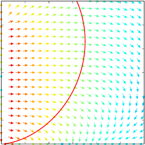
Figure 7. Energy-flux vectors when an external force is applied to small perpendicular wavenumbers (a) in the small-wavenumber range and (b) in the whole computational domain. The critical wavenumber and the Zeman wavenumber are, respectively, shown as red and cyan curves.

Weak-wave turbulence is expected to occur at wavenumbers where the linear wave period $\tau _{{w}} = (2\varOmega k_{\|}/k)^{-1}$ is much shorter than the eddy turnover time $\tau _{{e}} = (k^2 \bar {\varepsilon })^{-1/3}$. The critical wavenumber is evaluated to appear at $\tau _{{w}} = \tau _{{e}}/3$ in magnetohydrodynamic turbulence (Meyrand et al. Reference Meyrand, Galtier and Kiyani2016) and stratified turbulence (Yokoyama & Takaoka Reference Yokoyama and Takaoka2019). On the other hand, the Coriolis force affects little and isotropic Kolmogorov turbulence appears at the wavenumber range where the Coriolis period $\tau _{\varOmega } = (2\varOmega )^{-1}$ is larger than the eddy turnover time $\tau _{{e}}$. The separation wavenumber of isotropic Kolmogorov turbulence is known as the Zeman wavenumber $k_{\varOmega }$. A buffer range should exist between the critical wavenumber and the Zeman wavenumber. The curves representing the critical wavenumber (red) and the Zeman wavenumber (cyan) are shown in figure 7.

The energy-flux vectors at the wavenumber modes $k_{\|} \leq 50$ in the weak turbulence range are almost completely parallel to the $k_{\perp }$ axis, and the energy provided by the external force rarely goes to the modes $k_{\|} > 50$. Thus, the wavenumber modes at $k_{\|} > 50$ in the weak turbulence range have little energy. The minimal-norm vector can well reproduce the anisotropic energy flux in accordance with the resonant interactions among the inertial waves locally in wavenumber space.

The energy flux in the range where $\tau _{{w}} < \tau _{{e}}/3$ and weak-wave turbulence is expected to exist does not necessarily demonstrate a perpendicular flux. This results from the fact that the wavenumber modes at $k_{\|}>50$ have little energy and the modes in the range are subordinate to the modes at $k_{\|}<50$ having much larger energy.

The energy-flux vectors turn in direction near the wavenumber modes having $\tau _{{w}} = \tau _{{e}}/3$. In this case, the energy flux along the critical wavenumbers that gives the isotropisation of energy in the buffer range is not observed. In fact, the energy transferred via the resonant interactions moves on to the two-dimensional modes $k_{\|} = 0$.

The integrated energy fluxes obtained from the three-dimensional energy-flux vectors in the simulation where the external force is applied to the small perpendicular wavenumbers are almost equal to the corresponding integrated energy fluxes as shown in figure 8. The difference between $P_{\perp }^{{v}}$ and $P_{\perp }$ at small perpendicular wavenumbers $k_{\perp } < 6$ comes from the discreteness of the coarse-grained cell during the conversion from $P_x$ and $P_y$ to $P_{\perp }^{{v}}$ as seen in isotropic turbulence (figure 5). The difference between $P^{{v}}$ and $P$ at $k < 50$ where the external force has a direct effect comes from the discreteness of the coarse-grained cell during averaging the energy fluxes over the azimuthal angles or through the inner and outer surfaces of the cells. The negative parallel flux, $P_{\|}<0$, appearing at $k_{\|}<50$ where the external force affects shows that most of the energy provided by the external force goes to small parallel wavenumbers, and is dissipated there.

Figure 8. Perpendicular, parallel and isotropic integrated fluxes when an external force is applied to small perpendicular wavenumbers. The superscript $v$ denotes the integrated fluxes obtained from the three-dimensional energy-flux vectors. See also caption to figure 5.

3.2.2. Energy flux in DNS with isotropic forcing

Another DNS where more commonly used external force is employed is performed with $512 \times 512 \times 2048$ grid points. One may think that the resolution is not so high as that in recent high-resolution simulations. However, such high-resolution simulation is not easily performed because a long-time integration is required to obtain the weak inertial-wave turbulence where the energy is transferred by the resonant interactions.

Three-dimensional three-component random force is added isotropically to the small wavenumbers in $k_{{f}}-1/2 \leq |\boldsymbol {k}| < k_{{f}}+1/2$, where the forced wavenumber $k_{{f}}$ is set to $4$. In this DNS, the turbulent Reynolds number and the rotational Reynolds number are, respectively, evaluated as $Re_{{t}} \approx 1.6\times 10^2$ and $Re_{\varOmega } \approx 2.8$.

The energy spectrum as a function of the norms of wavenumbers obtained in the DNS is shown in figure 9. The energy spectrum at wavenumbers smaller than those of the external force $k_{{f}} \approx 4$ is as steep as $k^{-3}$. The two-dimensional flows, which are uniform in the direction parallel to the rotational axis, i.e. $k_{\|}=0$, account for a large fraction of the energy at small wavenumbers, though the number of two-dimensional modes is much smaller than that of the three-dimensional modes which have $k_{\|} \neq 0$. In fact, a large-scale columnar vortex is formed. Note that a statistically steady state can be achieved without small-wavenumber drag (Chan, Mitra & Brandenburg Reference Chan, Mitra and Brandenburg2012). At wavenumbers larger than $k_{{f}}$, the energy spectrum is dominated by three-dimensional flows, and is less steep than at small wavenumbers. In this energy spectrum, the isotropic Kolmogorov turbulence cannot be clearly observed, because the Zeman wavenumber is close to the Kolmogorov wavenumber as well as the cutoff wavenumber.

Figure 9. Energy spectrum, that given only by two-dimensional modes ($k_{\|}=0$) and that given by three-dimensional modes ($k_{\|} \neq 0$). The vertical line indicates the Zeman wavenumber.

The energy spectra are shown in figure 10. The spectra are close to the prediction of the weak turbulence theory, $E(k_{\perp }, k_{\|}) \propto k_{\perp }^{-5/2} k_{\|}^{-1/2}$, in the wavenumber range $4 \lessapprox k_{\perp } \lessapprox 30$ and $1/4 \lessapprox k_{\|} \lessapprox 4$. The abrupt drops at $k_{\|} \approx 4=k_{{f}}$ in the parallel-wavenumber spectra indicate that little energy is transferred to the large parallel wavenumbers $k_{\|} > k_{{f}}$ consistent with the weak turbulence theory. These spectra demonstrate that inertial-wave turbulence appears in the wavenumber range $4 \lessapprox k_{\perp } \lessapprox 30$ and $1/4 \lessapprox k_{\|} \lessapprox 4$.

Figure 10. Kinetic energy spectra (a) for each $k_{\|}$ as a function of $k_{\perp }$ and (b) for each $k_{\perp }$ as a function of $k_{\|}$.

The energy-flux vectors in the $k_{\perp }$–$k_{\|}$ plane in isotropically forced rotating turbulence are shown in figure 11. The energy-flux vectors roughly in the range $k_{\perp } \lessapprox 30$ and $k_{\|} \lessapprox 4$ are almost parallel to the $k_{\perp }$ axis. The perpendicular flux is consistent with the resonant interactions of inertial waves in the weak turbulence theory. In fact, the range where the perpendicular flux is observed corresponds to the range where the weak inertial-wave spectra are observed in figure 10.

Figure 11. Energy-flux vectors where an isotropic external force is applied (a) in the small-wavenumber range and (b) in the whole computational domain. See also the caption to figure 7.

On the other hand, the vector field of the energy flux has a sink at $(k_{\perp }, k_{\|}) \approx (100, 0)$. In this simulation, the energy flux along the critical wavenumbers predicted by the critical balance is not observed. This discrepancy is discussed in the next section.

To confirm the consistency of the energy-flux vectors with the commonly used integrated energy fluxes, the integrated fluxes are obtained from the three-dimensional flux vectors and compared with those obtained by (2.5) and (2.6) in figure 12. The isotropic and perpendicular fluxes obtained from the three-dimensional flux vectors are almost equal to those obtained by (2.5) and (2.6) except for the small wavenumbers $k, k_{\perp } < 8$. The difference at small wavenumbers comes from the discreteness of the cells and the averaging for $k_{\perp }$ and $k$. The parallel flux obtained from the three-dimensional flux vectors and the corresponding integrated flux are the same within the convergence criterion adopted in the GMRES method. These agreement and disagreements have been seen in the energy flux in HIT (figure 5b). Therefore, the energy-flux vectors are consistent with the integrated energy fluxes, which have been usually used in anisotropic turbulence.

Figure 12. Perpendicular, parallel and isotropic integrated fluxes in isotropically forced rotating turbulence. The superscript $v$ denotes the integrated fluxes obtained from the three-dimensional energy-flux vectors. See also the caption to figure 5.