2.1. Young–Laplace equation

This study examines a liquid pendant drop suspended from the outlet of a cylindrical needle, as depicted in figure 1. The drop is deformed by a uniform vertical airflow with velocity U _∞ to form a contact angle $\psi_{c}$ with the needle. Let a and h represent the outer radius of the needle outlet and the height of the drop, respectively. Assuming axisymmetry, the equilibrium shape of the drop can be described in two-dimensional (x,z) coordinates, with the origin at the centre of the needle outlet. Here, the x-axis denotes the radial direction, and the z-axis points in the vertical upward direction. Note that x is always positive in both the left and right sides of the z-axis in figure 1. The shape can also be expressed in polar coordinates, where r is the distance from the origin, and θ is the polar angle measured from the negative z direction. In this configuration, the bottom apex of the drop is located at θ = 0 and z = −h.

Figure 1. An axisymmetric pendant drop suspended from a needle outlet, immersed in a surrounding uniform upward vertical flow.

The equilibrium shape of the liquid drop surface results from the balance between surface tension and the pressure difference across the surface. Gunde et al. (Reference Gunde, Kumar, Lehnert-Batar, Mäder and Windhab2001) derived the Young–Laplace equation for an axisymmetric pendant drop in a quiescent environment. In our study, we modify this equation by incorporating the aerodynamic pressure term to assess the impact of external airflow. This approach aligns with that of Beard & Chuang (Reference Beard and Chuang1987), who used a prescribed pressure distribution around a sphere to determine the shape of a falling raindrop. The pressure difference at the bottom of the drop is expressed as

(2.1) \begin{equation}{p^{(i)}}_{\theta =0}-{p^{(e)}}_{\theta =0}=\sigma \frac{2}{b_{0}},\end{equation}

where σ is the surface tension coefficient of the liquid, and b ₀ is the radius of curvature at the bottom. Here, p ⁽ⁱ⁾ and p ^(e) denote the internal and external pressures, respectively. The pressures at an arbitrary θ are given as

(2.2) \begin{align}&\qquad\qquad\quad p^{(i)}={p^{(i)}}_{\theta =0}-\rho _{d} g(h+z)\!, \end{align}

(2.3) \begin{align}& p^{(e)}={p^{(e)}}_{\theta =0}-\rho _{a}g(h+z)-\frac{1}{2}\rho _{a}U_{\infty }^{2}(\kappa (0)-\kappa (\theta ))\!. \end{align}

Here, $\rho_d$ and $\rho$ _a are the densities of the drop and air, respectively, g is the gravitational acceleration, and $\kappa$ (θ) is the aerodynamic pressure coefficient on the surface of the drop, defined as

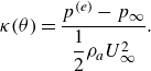(2.4) \begin{equation}\kappa (\theta )=\frac{p^{(e)}-p_{\infty }}{\dfrac{1}{2}\rho _{a}U_{\infty }^{2}}.\end{equation}

Expressions (2.3) and (2.4) are valid only under the assumption of inviscid flow, which is further explored in § 2.2. Subtracting (2.3) from (2.2) and using (2.1), we formulate the Young–Laplace equation for the pendant drop as

(2.5) \begin{equation}p^{(i)}-p^{(e)}=\sigma \left(\frac{1}{b_{1}}+\frac{1}{b_{2}}\right)=\sigma \frac{2}{b_{0}}-\left(\rho _{d}-\rho _{a}\right)g(h+z)+\frac{1}{2}\rho _{a}U_{\infty }^{2}(\kappa (0)-\kappa (\theta ))\!,\end{equation}

where b ₁ and b ₂ are the principal radii of curvature at a given point on the drop surface. Note that the hydrostatic pressure term includes (h + z) rather than (h − z) because the drop is located in the negative z-plane.

We can non-dimensionalise the equation with the radius of the needle. Defining dimensionless variables B ₁ = b ₁/a, B ₂ = b ₂/a, B ₀ = b ₀/a, H = h/a and Z = z/a, (2.5) is transformed into

(2.6) \begin{equation}\frac{1}{B_{1}}+\frac{1}{B_{2}}=\frac{2}{B_{0}}-{\textit{Bo}}_{a}(H+Z)+{\textit{We}}_{a}(\kappa (0)-\kappa (\theta ))\!,\end{equation}

where the Bond number and Weber number, based on the radius of the needle a, are defined as

(2.7) \begin{align}& {\textit{Bo}}_{a}=\frac{\left(\rho _{d}-\rho _{a}\right)\! ga^{2}}{\sigma }, \end{align}

(2.8) \begin{align}&\quad {\textit{We}}_{a}=\frac{\rho _{a}U_{\infty }^{2}a}{2\sigma }.\end{align}

Equation (2.6) is the final form of the Young–Laplace equation expressed with dimensionless variables. Notably, in (2.6), the dimensionless numbers Bo _a and We _a are independent of the droplet’s shape. Therefore, the solution process requires determining the aerodynamic pressure distribution $\kappa$ (θ) as well as the radii of curvature B ₁ and B ₂ of the equilibrium shape, necessitating a solution scheme for nonlinear equations.

2.2. Aerodynamic pressure distribution

To obtain the aerodynamic pressure distribution $\kappa$ (θ) around deformed pendant drop shapes, our numerical model remains simplistic by employing a concept of a Rankine ring source element, as depicted in figure 2(a). These ring sources are centred and distributed along the z-axis, encompassing both the drop and the extended needle in the positive z direction, as illustrated in figure 2(b). For the kth ring source, with intensity q _k and radius x _k at z = z _k , the velocity potential ϕ _k is derived following the approach of Hess (Reference Hess1962) and expressed as

(2.9) \begin{equation}\phi _{k}\left(x,z\right)=4q_{k}\frac{1}{\sqrt{Q_{1}}}K\left(\frac{Q_{2}}{Q_{1}}\right)\!,\end{equation}

where Q ₁ and Q ₂ are further defined as

Figure 2. The numerical scheme for calculating potential flow field around a pendant drop. (a) An irrotational flow field generated by an axisymmetric Rankine ring source combined with a uniform free stream. (b) Distribution of the ring sources used to model potential flow around the drop–needle system.

(2.10) \begin{align}& Q_{1}=\left(x+x_{k}\right)^{2}+\left(z-z_{k}\right)^{2}, \end{align}

(2.11) \begin{align}&\qquad\quad\,\, Q_{2}=4x_{k}x. \end{align}

Additionally, K( $\beta$ ), the complete elliptic integral of the first kind, is defined as

(2.12) \begin{equation}K\!(\beta )=\int _{0}^{\unicode{x03C0} /2}\frac{1}{\sqrt{1-\beta \sin ^{2} \theta }}\,\text{d}\theta ,\end{equation}

where $\beta$ is a non-negative real number. The flow velocity components are derived from the derivatives of ϕ _k with respect to the corresponding coordinates. The radial and axial velocity components of the axisymmetric flow, created from a set of ring sources combined with a uniform vertical free stream, is given as

(2.13) \begin{align}& u_{x}=\sum _{k}^{}\frac{\partial \phi _{k}}{\partial x}=\sum _{k}^{}2q_{k}\left[\frac{Q_{1}-x\left(x+x_{k}\right)}{x\sqrt{Q_{1}}\left(Q_{1}-Q_{2}\right)}E\left(\frac{Q_{2}}{Q_{1}}\right)-\frac{1}{x\sqrt{Q_{1}}}K\left(\frac{Q_{2}}{Q_{1}}\right)\right], \end{align}

(2.14) \begin{align}&\qquad u_{z}=U_{\infty }+\sum _{k}^{}\frac{\partial \phi _{k}}{\partial z}=U_{\infty }-\sum _{k}^{}4q_{k}\frac{1}{\sqrt{Q_{1}}\left(Q_{1}-Q_{2}\right)}E\left(\frac{Q_{2}}{Q_{1}}\right)\!, \end{align}

where E( $\beta$ ), the complete elliptic integral of the second kind, is defined as

(2.15) \begin{equation}E(\beta )=\int _{0}^{\unicode{x03C0} /2}\sqrt{1-\beta \sin ^{2} \theta }\,\text{d}\theta .\end{equation}

Determining the intensity, radius and position of each ring source is crucial for accurately simulating the axisymmetric flow around a specific drop shape. The boundary condition at the surface, comprising both the drop and needle, is given by

(2.16) \begin{equation}\boldsymbol{u}\boldsymbol{\cdot }\boldsymbol{n}=0,\end{equation}

where u = (u _x , u _z ) is the flow velocity vector, and $\boldsymbol{n}$ is the normal vector to the body surface. Employing a finite number of ring sources necessitates discretising the surface into an equal number of surface points ( $\xi_{m}$ , $\zeta_{m}$ ), at which (2.16) must be satisfied, as shown in figure 2(b). If x _k and z _k are fixed at specific values, then the velocity components in (2.13) and (2.14) become linear expressions with respect to q _k . In this case, (2.16) forms a system of linear equations that can be readily solved for q _k . Appropriate specification of the radius and position of each ring source significantly simplifies the determination of the potential flow field, thereby facilitating the calculation of the aerodynamic pressure distribution. In the current numerical model, the ring sources are uniformly distributed along the z-axis, with each source’s radius set so that it resides just inside the body surface. It has been determined that up to two hundred ring sources, as well as corresponding surface points, are sufficient to achieve a converged solution for the velocity potential.

Figure 3(a) displays an example of the potential flow field around a pendant drop with H = 4, where the stagnation point is located at the bottom apex of the drop, and the flow smoothly contours the surfaces of both the drop and the needle. It is important to note that this model does not account for any liquid flow inside the drop induced by the airflow, which, while affecting the internal pressure distribution, does not significantly alter the resultant equilibrium shape (Szakáll et al. Reference Szakáll, Mitra, Diehl and Borrmann2010).

Figure 3. Potential flow field and pressure distribution around a pendant drop. (a) Flow field around a drop with height H = 4. (b) Resultant aerodynamic pressure on the drop surface compared to potential flow around a sphere and experimental results from Fage (Reference Fage1936).

The resultant aerodynamic pressure distribution $\kappa$ (θ) around the drop is illustrated in figure 3(b) as a solid black line. For comparison, classical results of potential flow around a sphere and the empirical pressure distribution by Fage (1937), used in Beard & Chuang (Reference Beard and Chuang1987) for simulating raindrops, are also depicted. In general, the primary weakness of potential flow in describing the flow around a body is its inability to capture the pressure loss caused by flow separation. Imai (Reference Imai1950) demonstrated that using potential flow to describe spherical raindrops results in a significant overestimation of drop deformation, especially at the rear stagnation point, due to the full recovery of pressure. Consequently, Beard & Chuang (Reference Beard and Chuang1987) employed the empirical pressure data from Fage (1937) modified based on the potential flow to better represent flow separation and achieve a more accurate simulation of raindrop shape.

In the case of a pendant drop suspended from a needle, such pressure measurement data are unavailable in the literature. Thus we opted to utilise potential flow in an attempt to emulate the flow field around the pendant drop. Notwithstanding, figure 3(b) shows that the pressure on the downwind side of the pendant drop does not reach the stagnation pressure, $\kappa$ (θ) = 1. Therefore, we anticipate that the overestimation of aft pressure from potential flow is less significant for a pendant drop compared to a raindrop. As a result, the pendant drop shape emulated using potential flow is expected to more closely represent the realistic shape. Section 4.3 presents a comparison between the model results and experimental observations.

2.3. Approximate series solution

The general solution to the governing equation (2.6), which models the shape of a pendant drop, cannot be derived directly via algebraic methods due to mathematical complexities. The aerodynamic pressure term $\kappa$ (θ) lacks a straightforward explicit form in relation to the non-dimensional shape R(θ). The first principal radius of curvature, B ₁, is the radius of the circular arc that best approximates the curve R(θ) at a given point. The second principal radius of curvature, B ₂, is defined as the distance from a point on the drop surface to the z-axis in the direction perpendicular to the surface. We represent B ₁ and B ₂ as (Abbena, Salamon & Gray Reference Abbena, Salamon and Gray2017)

(2.17) \begin{align}& B_{1}=\frac{\left(R^{2}+R_{\theta }^{2}\right)^{3/2}}{R^{2}+2R_{\theta }^{2}-RR_{\theta \theta }},\end{align}

(2.18) \begin{align}& B_{2}=\frac{R\sin \theta \left(R^{2}+R_{\theta }^{2}\right)^{1/2}}{R\sin \theta -R_{\theta }\cos \theta },\end{align}

where R _θ and R _θθ are the first and second derivatives of R(θ) with respect to θ, respectively. Consequently, (2.6) is inherently nonlinear and necessitates iterative numerical methods. In this study, we develop a least-squares-based method to solve this equation. The approach begins by approximating the drop shape with a cosine series:

(2.19) \begin{equation}R(\theta )=\sum _{n=0}^{N}c_{n}\cos n\theta .\end{equation}

Here, N denotes a truncation order introduced to facilitate the numerical determination of the shape coefficients c _n . Assuming axisymmetry of the drop shape, the cosine series representation (2.19) ensures a smooth bottom apex at θ = 0, which can be imposed as the boundary condition (dR/dθ) _{θ = 0} = 0. The other geometric boundary conditions are specified as

(2.20) \begin{align}&\qquad\qquad R\left(\theta =0\right)=c_{0}+c_{1}+\cdots +c_{N}=H, \end{align}

(2.21) \begin{align}& R\left(\theta =\frac{\unicode{x03C0} }{2}\right)=c_{0}-c_{2}+c_{4}-\cdots +\left(-1\right)^{\left\lfloor N/2\right\rfloor }c_{2\left\lfloor N/2\right\rfloor }=1. \end{align}

Note that these conditions have already been non-dimensionalised using the radius of the needle, a. Equation (2.20) establishes the drop’s height, while (2.21) ensures contact with the needle outlet’s perimeter.

Employing a cosine series transforms the governing (2.6) into a nonlinear system concerning the shape coefficients c _n . If we incorporate the concept of surface points ( $\xi_{m}$ , $\zeta_{m}$ ) introduced in § 2.2, then the challenge of determining the equilibrium shape can be reformulated as

(2.22) \begin{align}f\left(\xi _{m},\zeta _{m};c_{0},c_{1},\ldots ,c_{N}\right)&=\frac{1}{B_{1}}+\frac{1}{B_{2}}-\frac{2}{B_{0}}+{\textit{Bo}}_{a}(H+Z)-{\textit{We}}_{a}(\kappa (0)-\kappa (\theta ))=0,\nonumber\\ m&=1,2,\ldots,M,\end{align}

where M is the number of surface points on the drop. The problem now translates to a system of nonlinear equations, represented as f = 0 concerning the shape coefficients c _n . The number of equations M and the number of unknowns N + 1 are independent. Therefore, the problem is solvable via an iterative nonlinear least squares method. This method is outlined as follows:

(2.23) \begin{align}&S=\sum _{m=1}^{M}f\left(\xi _{m},\zeta _{m};\boldsymbol{c}\right)^{2}+\boldsymbol{\lambda }^{\rm T}L\boldsymbol{c}, \end{align}

(2.24) \begin{align}&\qquad\qquad\frac{\partial S}{\partial \boldsymbol{c}}=\frac{\partial S}{\partial \boldsymbol{\lambda }}=0. \end{align}

In this context, S is an objective function that we aim to minimise, c = [c ₀ c ₁ … c _N ]^T is a column vector of shape coefficients, λ is a Lagrangian multiplier, and L is a 2 × (N + 1) linear constraint matrix given as

(2.25) \begin{equation}L=\left[ \begin{array}{c} 1\\ 1 \end{array} \begin{array}{c} 1\\ 0 \end{array} \begin{array}{c} 1\\ -1 \end{array} \begin{array}{c} 1\\ 0 \end{array} \begin{array}{c} 1\\ 1 \end{array} \begin{array}{c} 1\\ 0 \end{array} \begin{array}{c} \cdots \\ \cdots \end{array} \right].\end{equation}

This matrix consolidates the geometric constraints (2.20) and (2.21) into a single equation Lc = [H 1]^T, facilitating the use of height H as a geometric constraint to maintain linearity in the constraints. This is advantageous as more conventional metrics, such as volumetric diameter, would result in nonlinear constraint equations, complicating the numerical approach. Our approach enables the following iterative scheme for a nonlinear least squares problem:

(2.26) \begin{align}\boldsymbol{c}^{(i+1)}-\boldsymbol{c}^{(i)}&=-(\mathcal{J}^{T}\mathcal{J})^{-1}\mathcal{J}^{T}f\left(\boldsymbol{c}\right)^{(i)}\nonumber\\&\quad+(\mathcal{J}^{T}\mathcal{J})^{-1}L^{T}(L(\mathcal{J}^{T}\mathcal{J})^{-1}L^{T})^{-1} L(\mathcal{J}^{T}\mathcal{J})^{-1}\mathcal{J}^{T}f\left(\boldsymbol{c}\right)^{(i)}\!,\end{align}

where i is the iteration index, and Jacobian J, an $M\times(N+1)$ matrix, is defined via

(2.27) \begin{equation}\mathcal{J}_{mn}=\frac{\partial f_{m}}{\partial c_{n}}.\end{equation}

The iterative scheme (2.26) incorporates the Gauss–Newton method for nonlinear least squares problems in the constrained linear least squares estimator (Amemiya Reference Amemiya1985).

Due to the undefined explicit expression of $\kappa$ (θ) relative to c _n , the partial differentiation in (2.27) is calculated using a second-order central difference scheme. Our numerical model uses M = 200 surface points (equal to the number of ring source singularities inside the drop) and truncation order N = 100 for the cosine series. These values were determined based on convergence tests, which showed that further increases in M and N resulted in negligible changes to both the drop shape and the drag force arising from aerodynamic pressure. The iterative process, as specified in (2.26), continues until convergence of the shape coefficient vector c is achieved.

Figure 4. Equilibrium shapes of pendant drops at various sizes and Weber numbers.

The equilibrium shapes of pendant drops of various sizes under different flow velocities are presented in figure 4. Drop sizes range from H = 1 to H = 4, and the maximum flow velocity corresponds to Weber number We _a = 0.8. The maximum values of H and We _a used in the model calculations were chosen to match the experiment presented in § 4. In practice, drops larger than H = 4 tend to detach from the needle due to their weight, while flow velocities larger than that corresponding to We _a = 0.8 cause excessive vibration, also leading to drop detachment. The results in figure 4 indicate that aerodynamic pressure flattens the drop, akin to raindrop deformation observed by Beard & Chuang (Reference Beard and Chuang1987). As flow velocity increases, so does deformation, affecting the contact angle $\psi_{c}$ at the needle, which decreases with increasing drop size up to H = 3, but increases at H = 4 due to the weight of the drop. This trend in $\psi_{c}$ variation is consistent across different flow velocities.

Figure 5. Force balance on a pendant drop. (a) Different forces acting on the drop under the influence of surrounding flow. (b) Variation in forces with respect to drop size, with We _a = 0.8.

3.1. Vertical force equilibrium

The numerical model described in § 2 resolves the Young–Laplace equation for a pendant drop, thereby ensuring that the model accounts for the local force balance between pressure and surface tension on the drop’s surface. At equilibrium, this balance across the entire drop surface equates to a net zero force acting on the drop. Given the drop’s axisymmetry, horizontal components of force cancel each other, and only vertical forces are considered significant in this analysis. The vertical force equilibrium of the drop is expressed as

(3.1) \begin{equation}\varSigma F=F_{D}+F_{S}-\left(F_{G}-F_{B}\right)-F_{P}=0,\end{equation}

where subscripts D, S, G, B and P correspond to drag, surface tension, gravity, buoyancy and pressure, respectively. These forces, depicted in figure 5(a), are crucial for discussions regarding the stability and dynamic behaviour of the drop. Each force acts vertically and is expressed using dimensionless variables. The simplest among these is the surface tension force F _S , which pulls the drop upwards from its contact line with the needle. Given that the contact line is a circle with radius a, the net surface tension force is 2πσa sin $\psi_{c}$ . Non-dimensionalising this force by dividing by σa yields

(3.2) \begin{equation}F_{S}=2\unicode{x03C0} \sin \psi _{c}.\end{equation}

The net gravitational force, the weight of the drop minus the buoyancy, is non-dimensionalised in a similar manner as the surface tension force F _S . This expression is given as

(3.3) \begin{equation}F_{G}-F_{B}={\textit{Bo}}_{a} V,\end{equation}

where V represents the dimensionless volume of the drop. This force acts downwards, opposing the direction of the surface tension in (3.1).

The pressure force F _P results from the excess pressure at the needle outlet (Gunde et al. Reference Gunde, Kumar, Lehnert-Batar, Mäder and Windhab2001), analogous to the normal force on an object at a surface. This excess pressure is calculated by setting Z = 0 and θ = π/2 in the governing equation (2.6). As the force acts over the needle outlet area πa ², the dimensionless pressure force is given as

(3.4) \begin{equation}F_{P}=\unicode{x03C0} \left(\frac{2}{B_{0}}-{\textit{Bo}}_{a}H+{\textit{We}}_{a}\left(\kappa (0)-\kappa \!\left(\frac{\unicode{x03C0} }{2}\right)\right)\right)\!.\end{equation}

Finally, the drag force due to aerodynamic pressure around the drop F _D is derived by combining (3.1)–(3.4). Alternatively, this force can be calculated by integrating the pressure coefficient over the drop surface, expressed as

(3.5) \begin{equation}F_{D}={\textit{We}}_{a}\!\int \!\kappa (\theta )\hat{\boldsymbol{z}}\boldsymbol{\cdot }\text{d}\boldsymbol{A}={\textit{Bo}}_{a}V-\unicode{x03C0} \!\left(2\sin \theta _{c}-\frac{2}{B_{0}}+{\textit{Bo}}_{a}H-{\textit{We}}_{a}\left(\kappa (0)-\kappa\! \left(\frac{\unicode{x03C0} }{2}\right)\right)\!\right)\!,\end{equation}

where $\hat{\boldsymbol{z}}$ and d A denote a unit vector in the z direction and an infinitesimal area vector normal to the drop surface, respectively.

Once the drop shape is determined from the solution of the Young–Laplace equation, the relevant forces can be evaluated using the cosine series solution for the drop shape. For instance, figure 5(b) illustrates how vertical forces vary with drop size for We _a = 0.8. As the drop size increases, the surface tension force F _S changes with the varying contact angle $\psi_{c}$ . Consistent with the equilibrium shapes shown in figure 4, F _S initially decreases as the drop size increases and the contact angle decreases. However, as the drop becomes heavier, the contact angle increases again, and F _S begins to rise. Both the gravitational force F _G − F _B and the drag force F _D increase with the drop’s volume and cross-sectional area. Consequently, the pressure force F _P decreases to maintain force equilibrium as stated in (3.1). If the drop size is further increased beyond H = 4, detachment from the needle becomes likely as the pressure force approaches zero.

3.2. Stability criterion

In the equilibrium state, the pendant drop should theoretically maintain an axisymmetric shape as predicted by the numerical model described in § 2, given that the vertical forces are balanced as detailed in § 3.1. However, in practice, the drop may deviate from its vertical equilibrium position due to inherent instabilities. Such unstable motions have been documented by Dockery et al. (Reference Dockery, Aydin and Dickerson2024), who observed periodic motions of the pendant drop under external airflow, resembling the dynamics of a spherical pendulum rotating around the vertical axis. To evaluate the likelihood of such motions, it is essential to consider the stability of the equilibrium influenced by the combination of vertical forces.

This section utilises a similar approach to § 3.1, focusing on calculating torques rather than vertical forces to explain the drop’s tilting and oscillatory side motions. As a simplified method to determine equilibrium stability, we introduce a first-order perturbation by tilting the drop by a small angle $\varepsilon$ . Under such perturbation, the sum of the torques acting on the drop may not necessarily balance to zero. If the net torque exacerbates the tilting motion, then the equilibrium is deemed unstable, leading to further tilting in the direction of the disturbance. Conversely, if the net torque opposes the disturbance, then it indicates a return to stable vertical equilibrium.

Figure 6(a) depicts several torques influencing the drop under tilting motion. The drag force F _D , acting upwards, generates a torque that intensifies the tilting motion. Conversely, the gravitational force F _G − F _B (the net effect of weight minus buoyancy), acting downwards, serves as a restoring torque that pulls the drop back towards equilibrium. Assuming that the aerodynamic pressure distribution $\kappa$ (θ) remains constant for a small tilt angle $\varepsilon$ , the torques due to drag T _D and gravity T _G are described as

Figure 6. (a) Torques acting on a tilted pendant drop, shown along with the corresponding relative forces. (b) The value of (dΣT/d $\varepsilon)_{\varepsilon = 0}$ at different flow velocities. Stability of the equilibrium is determined by whether the net torque becomes positive or negative, with the critical heights $H_1^*$ and $H_2^*$ serving as stability criteria.

(3.6) \begin{align}& T_{D}={\textit{We}}_{a}\int Z\varepsilon \kappa (\theta )\hat{\boldsymbol{z}}\boldsymbol{\cdot }\text{d}\boldsymbol{A}, \end{align}

(3.7) \begin{align}&\quad\,\,\, T_{G}=-{\textit{Bo}}_{a}\int Z\varepsilon \text{d}V. \end{align}

Here, area and volume integrals are computed over the entire drop. Notably, T _G is negative, opposing T _D , and accounts for both weight and buoyancy as reflected in Bo _a , which includes ( $\rho$ _d − $\rho$ _a ).

Additionally, the surface tension force generates torque due to variations in the contact angle along the tilted drop’s contact line. Considering only the first-order tilting perturbation, the torque due to surface tension T _S is explicitly calculated as

(3.8) \begin{equation}T_{S}=\int _{-\unicode{x03C0} }^{\unicode{x03C0} }\frac{\cos \varphi }{\sqrt{1+\left(\varepsilon \cos \varphi +\cot \psi _{c}\right)^{2}}}\,\text{d}\varphi ,\end{equation}

where $\phi$ is the azimuthal angle around the z-axis (refer to Appendix A). Typically, the integration result is negative for cot $\psi_{c}$ > 0, indicating that the surface tension torque acts alongside gravitational torque as a restoring force. These torque expressions (3.6)–(3.8) are non-dimensionalised similarly to those in § 3.1. The condition for stable equilibrium is then formulated as

(3.9) \begin{equation}\left.\frac{\text{d}{\varSigma T}}{\text{d}\varepsilon }\right| _{\varepsilon =0}=\left.\frac{\text{d}}{\text{d}\varepsilon }\left(T_{D}+T_{G}+T_{S}\right)\right| _{\varepsilon =0}\lt 0,\end{equation}

which, after a few algebraic steps, simplifies to

(3.10) \begin{equation}{\textit{We}}_{a}\int Z\kappa (\theta )\hat{\boldsymbol{z}}\boldsymbol{\cdot }\text{d}\boldsymbol{A}-{\textit{Bo}}_{a}\int Z\text{d}V-\unicode{x03C0} \cos \psi _{c}\sin ^{2} \psi _{c}\lt 0.\end{equation}

Due to the complexity of explicitly formulating the integral terms in (3.10) for varying drop shapes and flow velocities, these terms are evaluated numerically. Figure 6(b) shows the value of $({\rm d}\varSigma T/{\rm d}\varepsilon)_{\varepsilon=0}$ as a function of drop height for different Weber numbers. At lower Weber numbers (We _a = 0.2 and 0.4), the net torque initially indicates stability with a negative ΣT value for smaller drops. As the drop size increases, the net torque becomes positive at a critical height $H_1^*$ , indicating instability predominantly due to the increasing influence of drag T _D over gravitational torque T _G . The recovery torque due to surface tension is limited due to small deformation at lower flow velocities, keeping the contact angle near π/2. This trend shifts when the flow velocity increases to We _a = 0.6, where the net torque ΣT begins to decrease as the drop size exceeds H = 3, suggesting a potential recovery of stability for larger drops.

Further increasing the flow velocity to We _a = 0.8 reveals a second critical height $H_2^*$ . Initially, the equilibrium is unstable for smaller drops due to significant torque T _D from the high-speed flow. However, unlike the lower We _a scenarios, the net torque ΣT does not increase significantly as the drop size approaches H = 3. This deviation is primarily attributed to a substantial reduction in the contact angle $\psi_{c}$ , leading to an increase in surface tension torque T _S caused by the higher flow velocity. Further increasing the drop size results in ΣT decreasing towards negative values, restoring equilibrium stability. This transition aligns with the experimental findings of Dockery et al. (Reference Dockery, Aydin and Dickerson2024), where no asymmetric motion was observed under high flow velocities. The recovery of stability is mainly due to the domination of T _G over T _D as shape deformation lowers the drop’s centre of mass. Meanwhile, the influence of T _S diminishes as $\psi_{c}$ increases for large drops approaching H = 4.

Figure 7. Laboratory set-up of a vertical wind tunnel experiment. (a) Shadowgraph set-up, including a high-speed camera, an LED light source, and a syringe. (b) Image processing procedures for accurate drop edge detection and shape analysis.

4.1. Experimental set-up

To validate the accuracy of our numerical model in representing the dynamics of pendant drops, observations were conducted using a high-speed shadowgraph system in a vertical wind tunnel, as depicted in figure 7(a). The tunnel is powered by a centrifugal blower with maximum capacity 1280 W, generating flow velocities that significantly influence the shapes and dynamics of pendant drops. The airflow becomes fairly straight and steady after traversing a honeycomb structure, mesh arrangement and contraction section. Preliminary measurements with a hot-wire anemometer indicate that the flow within the test section is uniform and steady, exhibiting turbulence intensity <0.5 %. Flow velocity is precisely regulated by an electric inverter linked to the blower, maintaining a deviation of less than 1 % during the measurement period.

Drops of pure distilled water, released from a needle with radius 1.38 mm at the centre of the test section, were controlled via a precisely calibrated syringe pump. The maximum stable drop size was limited to H = 4, as larger drops could not maintain equilibrium due to their increased weight, consistent with the vertical force balance described in § 3.1. On the other hand, the flow velocity was capped at We _a = 0.8, as higher speeds induced excessive vibrations and subsequent detachment of the drops from the needle.

A shadowgraph system was set up to image the drop shapes, utilising an LED light source positioned behind a diffuse glass plate to illuminate the observation area. Images were captured using a high-speed camera set at 1000 Hz across from the light source, enabling the capture of the unstable dynamics of the drops. The image analysis process, illustrated in figure 7(b), involves reconstructing drop shapes using a partial-area-based subpixel edge location method (Trujillo-Pino et al. Reference Trujillo-Pino, Krissian, Alemán-Flores and Santana-Cedrés2013). This algorithm, through multiple smoothing and iterative processes, achieves an uncertainty of less than 0.2 pixels in locating boundaries. In our experimental set-up, the image resolution is 27 µm per pixel, and the diameter of the needle, denoted as 2a, corresponds to approximately 100 pixels. Consequently, the uncertainty associated with pixel-based edge detection is negligible when assessing the shape, size and dynamic motion of the drops.

Control over drop size was finely tuned using the syringe pump with minimum flow rate 0.1 µl min⁻¹. To counteract evaporation and maintain consistent drop sizes, the pump speed was adjusted between 2 and 5 µl min⁻¹, depending on the drop size and airflow velocity. For each set drop size, shadowgraph images were captured for several seconds, spanning a hundred oscillation periods of the drop. Additionally, another experiment was conducted at a flow rate of up to 100 µl min⁻¹ to observe real-time changes in drop shape and dynamics with increasing size.

The boundary of the drop, determined from subpixel edge detection, was used to calculate further metrics such as drop volume V and the centre of mass position, as well as the tilting angle θ_CM . To estimate the volume from a two-dimensional image, the horizontal cross-section of the drop is assumed to be circular. Although this method introduces potential inaccuracies due to horizontal oscillations and deformation, averaging the volume over a prolonged period yields a reliable measure of the drop’s volume (Jones & Saylor Reference Jones and Saylor2009). The experiment employed this method to calculate the volume of the drop in both equilibrium and during unstable motions.

Furthermore, the axis ratio $\alpha$ of the drop was calculated as

(4.1) \begin{equation}\alpha =\frac{H}{\max \{W(z)\}},\end{equation}

where W(z) is the width of the drop at vertical position z (see figure 7 b). The axis ratio, a common measure for assessing the degree of deformation in liquid drops (Beard & Chuang Reference Beard and Chuang1987; Rimbert et al. Reference Rimbert, Escobar, Meignen, Hadj-Achour and Gradeck2020), serves as a crucial parameter for comparing the drop shapes derived from both the numerical model and experimental observations.

4.2. Pendant drop in quiescent flow

Previous studies, such as those by Gunde et al. (Reference Gunde, Kumar, Lehnert-Batar, Mäder and Windhab2001), have explored the equilibrium shape of pendant drops in the absence of an external flow field. Mathematically, this involves solving (2.6) without incorporating the aerodynamic pressure distribution term on the right-hand side. Solutions to this version of the equation have been obtained using the Runge–Kutta method, as demonstrated by Beard & Chuang (Reference Beard and Chuang1987) and Gunde et al. (Reference Gunde, Kumar, Lehnert-Batar, Mäder and Windhab2001). However, the current study employs a nonlinear optimisation scheme to determine the equilibrium shape for a discretised body surface, which is particularly useful when including the aerodynamic pressure term. Despite its utility, this method can result in physically incorrect interpretations as global optimisation of the least squares scheme is not always guaranteed. To evaluate the reliability and consistency of our numerical approach, we first compare the results of the numerical model under quiescent flow conditions with experimental outcomes to validate the effectiveness of the optimisation method in solving the highly nonlinear Young–Laplace equation.

Figure 8. Shadowgraph images of pendant drops under quiescent flow conditions, with corresponding equilibrium shapes calculated from the numerical model shown as dashed yellow lines.

Figure 8 presents a direct comparison between the shadowgraph image of a stationary pendant drop in quiescent flow and the equilibrium shape calculated from the numerical model. Qualitatively, the model exhibits an excellent resemblance to the realistic shape, particularly at varying drop sizes. The experimental observations confirm the increase in contact angle at larger drop sizes, as discussed in § 2.3. Quantitative comparisons, depicted in figure 9, show that the increase in axis ratio $\alpha$ with drop size – attributable to vertical elongation due to gravity – is consistently mirrored by the numerical model. Furthermore, the model accurately reflects the dimensionless volume of the drop observed experimentally. Therefore, we conclude that the least squares optimisation method successfully describes the equilibrium shape of the drop, validating its application in solving the Young–Laplace equation.

Figure 9. Comparison between experimental and numerical model results under quiescent flow conditions for (a) volume, (b) axis ratio of the drop.

4.3. Dynamic motions and stability criterion

Contrary to conditions of quiescent flow, the presence of an external flow induces additional deformation of the drop, as well as unstable motions. To capture this, the drop shape is observed over an extended period, and its trajectory across the two-dimensional image plane is consolidated into a single image that illustrates the general position and periodic movements of the drop. Figure 10 displays these observations as black and white images, where each pixel’s value indicates the likelihood of the pixel being within the drop boundary, thereby visualising both the general drop shape and the directional tendencies of its motions. The equilibrium shapes calculated by the numerical model, using the same drop size and flow velocity conditions, are superimposed as yellow dashed lines. Qualitatively, the model closely predicts the time-averaged drop shape, lying within the outlined black and white areas. In many cases, the drop appears to oscillate sideways, exhibiting the projection of three-dimensional conical pendulum motion, referred to as the (1a, 0) mode by Dockery et al. (Reference Dockery, Aydin and Dickerson2024). This region of equilibrium instability is observed within certain ranges of drop size and flow velocity, consistent with the concept of critical heights outlined in § 3.2.

Figure 10. Experimental results of pendant drop shapes in air flows of varying velocity: (a–d) We _a = 0.2, (e–h) We _a = 0.4, (i–l) We _a = 0.6, (m–p) We _a = 0.8. Dashed yellow lines indicate equilibrium shapes calculated from the numerical model.

At a low flow velocity We _a = 0.2, smaller drops remain stable at their equilibrium positions (figures 10 a,b). However, as the drop size exceeds the critical height $H_1^*$ , the drop begins to exhibit unstable motion around the vertical axis, maintaining an axisymmetric shape on average (figures 10 c,d). A similar phenomenon occurs at a higher flow velocity of We _a = 0.4, where $H_1^*$ is relatively lower, and the drop becomes unstable earlier as its size increases (figure 10 f). With further increased flow velocity to We _a = 0.8, a second critical height $H_2^*$ emerges, where the drop regains stability and no longer deviates from the vertical axis (figure 10 p). Under this condition, the drop oscillates vertically due to the reduced influence of surface tension, yet remains in an axisymmetric shape, and is thus considered stable, aligning with predictions from the numerical model in § 3.2.

Similar to quiescent flow scenarios presented in § 4.2, the volume and axis ratios of the drop are quantitatively compared with the numerical model in figures 11(a,b), respectively. Since the drop is not stationary and exhibits periodic motion, each data point in figure 11 is based on the mean drop shape, obtained by averaging the instantaneous shape R(θ) in polar coordinates over 5000 images spanning at least 50 oscillation periods. The experimental data align well with the model, showing an increase in volume and a decrease in axis ratio at the same drop height with increasing flow velocity. However, at We _a = 0.6, slight deviations are noted, attributed to difficulties in assessing equilibrium shapes from time-averaged data when the drop exhibits both unstable pendulum motions and vertical oscillations (see figure 10 l).

Figure 11. Comparison between experimental results and numerical model for pendant drops in air flow: (a) volume, (b) axis ratio of the drop.

It is worth noting that the excellent agreement between simulation and experiment is not unexpected, despite the assumption of potential flow in the numerical model. Although potential flow does not account for possible flow separation around the drop, the results of Beard & Chuang (Reference Beard and Chuang1987) and Rimbert et al. (Reference Rimbert, Escobar, Meignen, Hadj-Achour and Gradeck2020) emphasise the critical importance of modelling the foreface pressure distribution using potential flow in order to reproduce the characteristic flattened shape of deformed drops. In their studies, drop deformation was successfully predicted for Reynolds numbers up to O(10³) and Weber number up to O(1). In our study, the maximum Weber number based on drop height is We _H = 3.2, corresponding to Re _H = 2540, which falls within a range similar to that of previous studies. This suggests that our numerical model is well suited to the current scope of the drop–airflow system.

More quantitative observations of changes in equilibrium stability and the existence of the two critical heights $H_1^*$ and $H_2^*$ are obtained by deliberately increasing the drop size over time. Figures 12 and 13 display the tilting angle θ_CM relative to changing drop size. Figure 12 plots each data point as the root mean square value of θ_CM as it fluctuates over time, while figure 13 presents instantaneous tilting angles against drop height. Given that the periodic motions result in large fluctuations of the tilting angle, the equilibrium stability of the drop is clearly evident in these graphs. Both experiments consistently delineate regions of stable and unstable equilibria. As flow velocity increases, $H_1^*$ decreases due to stronger aerodynamic pressure even at smaller drop sizes. At high velocities, the second critical height $H_2^*$ appears at later stages when the drop size is larger, and the equilibrium regains its stability, as observed in cases whereWe _a = 0.8. Notably, slight fluctuations of θ_CM in stable regions for We _a = 0.4 and We _a = 0.8 are due to vertical oscillations. It is important to note that fluctuations in the tilting angle are sometimes suppressed even under unstable conditions (see figures 13 d,e), suggesting that the internal flow induced by the high volume flow rate of the syringe pump as the drops continue to grow in size may impact the dynamic behaviour of the drop. However, such phenomena are not observed in figure 12 when the drop size is maintained constant.

Figure 12. Root mean square value of tilting angle θ_CM measured in shadowgraph experiments: (a) We _a = 0 (quiescent flow), (b) We _a = 0.2, (c) We _a = 0.4, (d) We _a = 0.6, (e) We _a = 0.8. Each data point marked with a circle symbol represents the measured tilting angle for a specific drop size.

Figure 13. Variation of tilting angle θ_CM over time while gradually increasing the drop size using a syringe pump: (a) We _a = 0 (quiescent flow), (b) We _a = 0.2, (c) We _a = 0.4, (d) We _a = 0.6, (e) We _a = 0.8.

An interesting observation from figure 13 is that the angular amplitude of unstable motion (defined as the difference between the maximum and minimum values of θ_CM ) remains relatively consistent across a wide range of flow velocities and drop sizes. This suggests that despite significant variations in drop deformation and drag force, the extent of tilting does not change drastically. While our current force balance model effectively captures the onset of instability, it is limited in explaining the dynamics of significantly tilted drops, where asymmetry and three-dimensional effects become important. As previously explored by Dockery et al. (Reference Dockery, Aydin and Dickerson2024), one may attempt to model the conical pendulum-like motion using a balance of surface tension, gravity, drag and centrifugal forces. However, estimating the drag force on a tilted drop is challenging, as the surrounding flow field would differ significantly from that around an axisymmetric configuration. Additionally, the difficulty of capturing the three-dimensional shape of a highly tilted drop further complicates the evaluation of surface tension effects. Further investigation into the tilting angle of the drop will likely involve numerical studies incorporating realistic simulations of unsteady flow fields and drop motion.

Regarding stability of the equilibrium, all experimental data can be integrated to obtain figure 14(a), which presents a stability regime map of the pendant drop. This map uses data points to indicate whether the drop at a specific height and flow velocity exhibits stable or unstable equilibrium, while the solid black line and dashed red line denote the predicted critical heights $H_1^*$ and $H_2^*$ , respectively. The equilibrium is considered stable when the root mean square of the tilting angle θ_CM is less than 0.1 rad. This threshold value provides a statistically robust separation between data with small and large θ_CM,RMS , as shown in figure 14(b). The experiment corroborates the model’s results, as $H_1^*$ decreases with increasing flow velocity, and $H_2^*$ emerges at high velocities. In the case We _a = 0.68, the drop appears to be in an unstable equilibrium despite exceeding the second critical height $H_2^*$ , possibly due to excessive vertical movement, which slightly increases the tilting angle. Nonetheless, the model effectively explains the stability behaviour observed in the experiments, thus validating the present numerical model and vertical force balance analysis in §§ 2 and 3 for predicting whether the drop exhibits unstable periodic motion or remains stationary with a deformed equilibrium shape.

Figure 14. (a) Stability regime map based on experimental data, complemented by predictions from the numerical model. Symbols indicate whether the equilibrium is stable or unstable at specific drop sizes and flow velocities. Curves representing the two critical heights $H_1^*$ and $H_2^*$ , as calculated from the numerical model, are shown with a solid black line and a dashed red line, respectively. (b) A histogram of θ_CM,RMS values from experimental cases, with a dashed line marking the stability threshold.

To complete the discussion of the model’s prediction of instability, it should be noted that the observed periodic unstable motion is unlikely to result from vortex shedding caused by flow separation. Beard & Kubesh (Reference Beard and Kubesh1991) proposed the possibility of resonance between the oscillatory motion of falling water drops and vortex shedding behind the drop. For small drops approximately 1 mm in diameter, the shedding frequency often matches the natural frequency of oscillation. However, the drops studied here are relatively larger, exhibiting oscillation frequencies below 60 Hz, while the expected vortex shedding frequency in this regime exceeds 100 Hz. Thus we find no compelling evidence of strong resonance or coupling between drop oscillation and vortex shedding due to flow separation. Furthermore, the numerical study by Agrawal et al. (Reference Agrawal, Premlata, Tripathi, Karri and Sahu2017) reported that for drops in systems with a high liquid-to-air viscosity ratio, vortex shedding does not break azimuthal symmetry. Therefore, although unsteady forcing from flow separation exists in reality, it is more likely that the onset of instability from the vertical, axisymmetric equilibrium position results from the balance between several relevant forces.