


1. Introduction
One of the defining features of granular materials is their so-called static yield stress, which means that sufficient forcing is required for irreversible plastic flow to occur. This feature is thought to underpin the stationary stability of many aggregates with inclined surfaces, such as hillsides, sand dunes and gravel heaps. Understanding the boundaries between yielding and static material is also vital when failure does occur. Debris flows, snow avalanches and pyroclastic density currents have greater destructive potential when a larger proportion of material is involved in dense fluid-like flow, so any model for their prediction must be able to capture this aspect. Here, discrete particle simulations are used to test a mathematical theory for granular flow in order to illuminate general features of the solid-like to fluid-like transition. A simple prototypical geometry is considered in which hard spherical grains, falling due to gravity, are confined between frictional vertical sidewalls. Pertinently, a steady flow regime is identified in which a region of approximately unyielding material coexists with surrounding regions containing fast flowing grains. Provided that the mean grain packing density is below jamming but above the threshold for dense flow, fluid-like shear zones are found close to the walls and a high-density creeping plug occupies the centre of the pipe. This flow structure is present in multiple geometries suggesting that the underlying physical basis is important for a wide range of related flows.
Motivation for the present study also comes from the industrial flow of powders and grains in standpipes, hoppers and silos. Not only is the vertical chute of interest as a purely rheometric device, it is a common and important component of many practical apparatus. As such, the first investigation presented here is the flow in a standpipe connecting two hoppers, which, for example, is a common configuration in catalysis (Geldart & Radtke Reference Geldart and Radtke1986), pebble-bed (Rycroft et al. Reference Rycroft, Grest, Landry and Bazant2006) and fluidised bed reactors (Srivastava et al. Reference Srivastava, Agrawal, Sundaresan, Karri and Knowlton1998). In this arrangement the upper hopper feeds the standpipe which then transports material to the outlet hopper at the bottom. In practise, provided there is sufficient supply at the top, the opening angle and length of the outlet hopper walls are the primary control parameters for the mass flux and hence for the observed dynamics. Here, attention will be limited to outlet hoppers which lead to a long-time steady uniform dynamics. This class of flow within conical hoppers is well studied, both experimentally (see e.g. Nedderman et al. Reference Nedderman, Tüzün, Savage and Houlsby1982; Knowlton, Mountziaris & Jackson Reference Knowlton, Mountziaris and Jackson1986) and theoretically (Jenike Reference Jenike1964; Gremaud, Matthews & Shearer Reference Gremaud, Matthews and Shearer2000; Sun & Sundaresan Reference Sun and Sundaresan2013). Therefore, in the present study, the outlet hopper is simply taken as a flux-control device leaving the focus here on the standpipe flow.
Due to its geometric simplicity, there are many previous works describing flow in vertical chutes. However, certain key features of the present study make our findings and analysis distinct. Firstly, the conical outlet hopper contrasts certain experimental set-ups (e.g. Nedderman & Laohakul Reference Nedderman and Laohakul1980; Moka & Nott Reference Moka and Nott2005) which have instead used a variable width orifice located in the centre of a flat basal wall. This arrangement naturally leads to non-uniform flow because the effects of matching with the outlet flow are observed for a considerable distance into the pipe, an aspect which is minimised by the converging outlet. Secondly, many previous studies (e.g. Pouliquen & Gutfraind Reference Pouliquen and Gutfraind1996) report a slip velocity along the sidewalls whereas here sufficiently rough walls, made from fixed particles, are used in order to suppress slip. This is done due to the known complexities of constitutive modelling with smooth walls (see Shojaaee et al. (Reference Shojaaee, Roux, Chevoir and Wolf2012) for a discussion). These distinctions lead to flow in the shear zones classified as ‘inertial flow’ in the spirit of the regime distinctions outlined by Chialvo, Sun & Sundaresan (Reference Chialvo, Sun and Sundaresan2012) in which packing density, strain rate and coordination number lie between the limits of quasi-static and dilute flows.
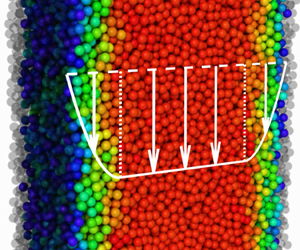
A demonstration of the novel structure of the vertical flow is provided in figure 1. This two-dimensional example makes clear the distinction between the inertial flow in the shear zones and the quasi-static flow in the central plug. In this simulation, and throughout this paper, the DEM ‘discrete element method’ (Cundall & Strack Reference Cundall and Strack1979), as implemented in the LAMMPS software (Plimpton Reference Plimpton1995), is employed. Broadly speaking, the motions of many grains are computed directly given accelerations due to body forces and contact forces. Flow is driven by gravity and a Hookean spring force, with a large stiffness, acts normally at the point of grain contacts along with a dissipative force that is proportional to the relative velocity. A complementary tangential force is also included in order to mimic Coulomb-type friction at the grain surfaces. DEM simulations allow flow fields and forces to be resolved at all times, measurements which are very difficult to achieve in physical experiments. In the illustrative example in figure 1 the domain is periodic in the gravity direction  $y$ and flow is confined between walls of frozen black particles. Flowing particles are coloured by the number of contacts they are currently making, the coordination number $Z$, and the resultant force vectors are plotted as centre-to-centre lines. This simulation snapshot effectively defines the inertial-dominated flows of interest in this paper because the mean value of $Z$ in the shear zones is below the critical value $Z_c^{2D}\simeq 3.4$ defined by Otsuki & Hayakawa (Reference Otsuki and Hayakawa2011) and Kruyt & Rothenburg (Reference Kruyt and Rothenburg2014) and the contact network is rearranging quickly. In the central plug, the contact number is above critical, placing the flow there in the locally quasi-static regime with a force network that is long lived and much more regular.

Figure 1. A snapshot of a two-dimensional DEM simulation in which the circular outlines of the flowing grains are coloured by their coordination number  $Z$ and the fixed wall particles are rendered with a black outline. Gravity points downwards and vectors of the contact forces are plotted as centre-to-centre lines with line widths scaled by force magnitude. A movie animation is available (see supplementary movies are available at https://doi.org/10.1017/jfm.2021.909).
Outside the range of inertial-dominated flows lie dilute flows, when the mass flow rate is high, and fully quasi-static regimes, for slow flows at low flux. Raafat, Hulin & Herrmann (Reference Raafat, Hulin and Herrmann1996) showed that non-uniform transient pulses dominate the dilute regime in long pipes and here a separation of the flow from the sidewalls is also observed. Gutfraind & Pouliquen (Reference Gutfraind and Pouliquen1996) studied the opposite regime of fully quasi-static flow using a basal plate that moved slowly downwards to enforce a creeping flow. Their results exhibit large packing fractions and a highly connected contact network throughout the system, even in the shearing regions. Intriguingly, this state cannot be replicated in either periodic cells or in the hopper-controlled set-up considered here as both approaches lead to a jammed static assembly. However, significant transient pulses are observed here even before this jamming limit is reached. These findings demonstrate that the favourable steady uniform regimes crucially rely on the shear zones being in the inertial regime. This feature is exploited here both via further idealisations of the DEM modelling as well as through continuum modelling.
As suggested by the illustrative simulation shown in figure 1, the steady flow in a standpipe between two hoppers can be well approximated by the flow in a periodic cell. Here, this non-trivial step is first realised by directly extracting a section of pipe from the full three-dimensional hopper-controlled set-up and placing it in a periodic simulation domain. Because the long-time dynamics is very close to the initial conditions, the role of the hoppers is found to be limited to setting the flow rate only. For the periodic cells, this means that the mean solid volume fraction is the only remaining parameter controlling the flow regime. In addition to rough planar-parallel walls, flows in cylindrical pipes are also considered here. These periodic simulations are also fully three-dimensional, with walls constructed from particles frozen in an axisymmetric annulus, and provide a key additional test case to assess the robustness of the vertical flow features.
Due to a close match between full hopper-controlled DEM simulations and those in equivalent periodic cells, a further novel idealisation is made here. A cubic domain is introduced in which all of the walls are periodic with their opposites. Vertical chute flow is then replicated by subjecting particles in one half of the domain to an upward-pointing gravitational force, and those in the other half to a downward force of the same magnitude. These conditions generate a counter-flow, which at steady state is found to give zero vertical velocity at the sidewalls and mid-point and leads to an approximate equipartition of particles in each half of the domain, despite their freedom of motion. This has many advantages and overcomes certain limitations inherent in many previous related studies. As well as the difficulties of constitutive modelling close to rigid boundaries, there are also complexities which arise when coarse graining the DEM fields to generate continuum fields (see Weinhart et al. Reference Weinhart, Thornton, Luding and Bokhove2012). Furthermore, precise control of the mean solid volume and chute width can be achieved due to the geometrically regular, rather than bumpy, flow region.
Progressive close matching of the DEM results between each of the geometries forms an unbroken link between realistic flow and the idealisations required for mathematical analysis. The major result of this paper is then the derivation of exact solutions for the flow within the shear zones, close to the pipe walls, in both parallel and cylindrical geometries. These novel continuum solutions are based solely on mass and linear momentum balances using the  $\mu (I)$, $\varPhi (I)$-rheology of Pouliquen et al. (Reference Pouliquen, Cassar, Jop, Forterre and Nicolas2006). In this theory, both the steady solid volume fraction $\varPhi$ and the ratio of shear to normal stress $\mu$ are taken to be functions of the inertial number $I$, which is a non-dimensional strain rate designed to reflect the frequency of grain rearrangements. These relations are well verified for many important flows (see GDR MiDi 2004), but, to date, more attention has been applied to the incompressible $\mu (I)$-rheology of Jop, Forterre & Pouliquen (Reference Jop, Forterre and Pouliquen2006) in which $\varPhi =\phi _*$ is a constant. This limitation of the incompressible theory actually prohibits application to vertical pipe flow as no unique pressure solution exists. As in the DEM simulations, the mean solid volume fraction $\phi _0$ is the key parameter controlling the steady flow in a given pipe, making the $\varPhi (I)$ relation a reassuring closure for the problem formulation.
Given the exact solutions for the variation of vertical velocity and solid volume fraction across the chute, simple scaling laws are established which link all of the control parameters to the resulting bulk flow. In particular, inputting  $\phi _0$ and the chute width $W$ gives the pressure, mass flux and shear zone width $\delta$. Conversely, these relations can be easily inverted to find the mean packing density, velocities and pressures in a pipe that is subject to a fixed mass flow rate. The duality in this regard, as well as parallels between cylindrical and rectangular pipes, suggests a universality of the relations and inspires direct application in practical scenarios.
2. Discrete particle simulations
The DEM is employed here to provide data for model comparison and hypothesis testing. Specifically, the LAMMPS software (Plimpton Reference Plimpton1995) is used to simulate the motion and interactions of many spherical grains. As described in table 1, idealised systems of perfectly monodispersed particles of unit diameter  $d$ and intrinsic density $\rho _*$ are considered here. Contact laws, which mediate interactions, and the related parameters are taken from Silbert et al. (Reference Silbert, Ertaş, Grest, Halsey, Levine and Plimpton2001) because they have been found to replicate many experimental results, such as granular flow down a frictional inclined plane (see GDR MiDi (2004) for a summary). The normal contact force consists of a Hookean linear spring, with stiffness $k_n$, compressed by the normal overlap distance, and a dissipative dashpot, with damping $\gamma _n$, which scales linearly with the relative normal velocity and particle mass. Tangential forces, with parameters denoted with subscript $t$, follow a similar arrangement, but with accumulated horizontal displacement being used in place of the overlap. Grain surface friction is then replicated by truncating this tangential force by the normal force scaled with $\mu _p$ i.e. a grain-scale Coulomb yield criteria. A fixed timestep $\delta t=1\times 10^{-4}$ and constant gravitational acceleration magnitude $g$ are used in all simulations presented here. All DEM data will be presented as coarse-grained continuum fields, as described in appendices A and B, unless stated otherwise.
Table 1. Parameters used in the discrete particle simulations.
2.1. Flow in the standpipe connecting two hoppers
As shown in figure 2, the DEM study begins with simulations of a hopper-fed vertical pipe with a converging bottom outlet, with each component being constructed from pairs of planar walls. The upper feed hopper has two flat walls of length  $L_{in}=121d$ opening with angles $\theta _{in}$ relative to the horizontal axis and joining the top of the pipe at $y=0$. The lower outlet is also composed of two flat walls converging with angles $\theta _{out}$ and has a fixed drop-height $L_h=50d$. This outlet attaches to the bottom of the parallel chute walls which are located at $x=0$ and $x=W$ for $y\in [0,L_p]$, where length $L_p$ is the pipe length. Unlike the hopper walls, the walls of the chute are geometrically roughened by affixing particles which remain static throughout the simulation. These frozen wall particles, which are otherwise identical to the flowing particles, do not overlap with one another and have centres approximately uniformly randomly distributed in $x\in [-d/2,d/2]$ and $x\in [W-d/2,W+d/2]$. Periodic walls are placed in the third direction $z\in [0,L_z]$ where $L_z=10d$ is chosen to minimise computational expense whilst allowing the flow to be fully three-dimensional. Provided that sufficient inflow is available at the top, the primary parameters controlling the mass flux out of the system are $\theta _{out}$ and $W$, which in turn set the outlet opening width $\varDelta$.

Figure 2. DEM particles coloured by vertical velocity in the hopper-controlled set-up after a steady circulating flow has been established. Here, the frozen particles which make up the wall have been rendered translucent black, as have the hopper walls. This example is for a chute width  $W=30d$, depth $L_z=10d$ and with a short pipe length $L_p=200d$, chosen for illustrative purposes. The upper inflow hopper opens with angle $\theta _{in}=65^\circ$ whereas the lower outflow hopper has $\theta _{out}=80^\circ$ giving an outlet opening $\varDelta =12.5d$. It should be noted that the velocity scale is limited in panel (b) to better contrast the spread of velocities within the chute. (a) Full simulation, (b) close-up view of the steady flow region and (c) close-up view of the outflow region.
To initialise the flow in the hopper system, the full geometry, including the pipe walls, is first constructed from impenetrable planar panels. The lower hopper is also blocked with an additional wall spanning the outlet. Particles are inserted randomly into this enclosed domain and allowed to settle, ensuring that a sufficient portion is filled. The pipe walls are then formed by freezing in place the particles within the thin wall regions, as illustrated by the black grains in figure 2. Subsequently removing the wall blocking the outlet then starts the gravity-driven flow. This set-up would naturally drain the initial finite mass of the system, leading to related transient effects. Instead, two methods of replenishing material in the upper feed hopper were explored. Firstly, fresh material was added by randomly placing new grains above the top free surface whilst material leaving the outlet was deleted. This worked well, but required tuning the rate of input to match the outlet flux. To overcome this, the domain was instead made periodic in the vertical direction such that material leaving the bottom outlet re-entered the domain just above the surface of the upper hopper material. As shown in figure 2, this set-up reaches a steady recirculating state that is approximately symmetric about  $x=W/2$.
Despite this symmetry in the cross-pipe direction, there is potential for much non-uniformity and unsteadiness in the downstream direction, as detailed in figure 3. For very narrow openings there is the possibility of jamming the outlet, either irreversibly or quasi-periodically, as has been widely studied in many granular systems (To, Lai & Pak Reference To, Lai and Pak2001; Zuriguel et al. Reference Zuriguel, Garcimartín, Maza, Pugnaloni and Pastor2005). Here, a snapshot is plotted in panel  $(a)$ of figure 3 of an outlet which is narrow but which does not jam irreversibly. In this case the velocity field and flow rate is clearly unsteady and non-uniform throughout the system. Panel $(c)$ in the same figure demonstrates that, in the opposite extreme, the fast flow rates caused by wide outlets may be steady in the laboratory frame but non-uniform in the flow direction. In this case the flow accelerates and detaches from the pipe walls generating a dense fast core surrounded by a very dilute gas. In the present work, the focus will be on the fully steady regions of intermediate flows, for example the one observed in panel $(b)$ of figure 3, which is equivalent to the set-up detailed in figure 2. Experimentation with the opening angle reveals that such flows exist in the approximate range $77^\circ \lesssim \theta _{out}\lesssim 83^\circ$, hence the remainder of this paper will focus on these regimes.

Figure 3. Snapshots of the fully developed flow in hopper-controlled systems with substantially different outlet opening angles. Note that the plotting axes have been rotated by  $90^\circ$ to aid illustration. A complementary movie animation is provided to illustrate the unsteady pulsing observed, in particular for the slow and fast flows shown in panels (a) and (c), respectively.
For set-ups tuned to generate an approximately steady uniform region, the noteworthy downstream trends which are summarised in figure 4 for a range of examples. As shown in panel  $(c)$ of figure 4, the max flux
 \begin{equation} Q_M = \rho_* L_z \int_0^W v(x)\phi(x) \,\textrm{d}\kern0.7pt x , \end{equation}
is strongly dependent on the outlet opening angle  $\theta _{out}$ and is effectively uniform throughout the system. However, as shown in panels $(a)$, $(b)$ and $(d)$, this constant flux of grains is achieved by a subtly varying flow in which the velocity, volume fraction and pressure slowly vary down the chute. These variations appear to reach a limiting asymptotic state in the range of $y$ that is bounded by the vertical dashed lines. The lack of significant pressure variation in the steady region of the pipe makes this flow distinct from the linear lithostatic variation observed in inclined plane flow. Known as the ‘Janssen effect’ (Janssen Reference Janssen1895), this signifies that the wall stress accommodates the weight of flowing material. Here, the maximal values of $\phi$ and $v$, which are located close to the chute centre $x=W/2$, are also approximately constant with $\mathrm {max}(\phi )$ close to random close packing $\phi _{rcp}$. It is also these regions for which the temporal fluctuations close to the inflow, indicated by the dashed range in panel $(a)$, are almost negligible. A closer study of these regions will be the focus of the next section.

Figure 4. Variation of the flow along the vertical pipe for three different outlet openings  $\theta _{out}$. Here, the remaining parameters are the same as in figure 2 except that a longer pipe $L_p=450d$ is used. The maximum vertical velocity $(a)$, the maximum solid volume fraction $(b)$, the mass flux $(c)$ and the mean value of the pressure $(d)$ are plotted as functions of the vertical coordinate. Dotted curves in panel $(a)$ indicate the range whereas the solid curves are the time-averaged values. For clarity, only the averaged values are given in the other plots. Vertical black dashed lines indicate the proposed steady region which is transferred to the rigid periodic cells. In panel $(b)$ the random close packing $\phi _{rcp}$ fraction is indicated by a red horizontal dashed line.
2.2. Approximation by vertical flow in a periodic cell
Here the full hopper-fed flux-controlled set-up is reduced to one-dimensional flow by matching with smaller periodic cells. To achieve this conversion the section of pipe in which the flow is approximately uniform downstream is copied and placed into a domain in which the vertical  $y$ direction is periodic. In essence this allows for the continuation of the flow development that would take place in a very long pipe. Indeed, the trends already observed in the full system, that the velocity increases and that particles migrate to the centre, are smoothly continued in these simulations. This allows for the long-time asymptotic steady state to be approximately realised, one which can be compared with time-independent solutions of the proposed equations. However, as will be seen during the model development, such steady solutions are sensitive to both the mean solid volume fraction $\phi _0$ and the width of the chute $W$. Because the walls of the pipe are constructed from frozen particles, which are irregularly spread over a range of $x$ at each wall, both the width and total volume that the flowing particles occupy are subject to uncertainties.
An alternative idealisation of vertical chute flow is made here which allows for precise control of the parameters  $\phi _0$ and $W$ and also guarantees that steady flow is accompanied by no slip at the sidewalls. This is achieved through a doubly wide domain containing two equally partitioned counter-flowing regions. This geometry is perfectly cubic with dimensions $x\in [0,2W]$, $y\in [0,L_y]$ and $z\in [0,L_z]$, and each boundary face is periodic with its opposite. A counter-flow, which represents two simultaneous vertical chute flows, is then driven by an asymmetric gravitational body force such that
 \begin{equation} \boldsymbol{g} = \begin{cases} g \boldsymbol{\hat{y}} & \text{for } 0\leq x < W , \\ -g \boldsymbol{\hat{y}} & \text{for } W\leq x < 2W , \end{cases} \end{equation}
where  $\boldsymbol {\hat {y}}$ is the unit vector in the vertical direction and $g$ is the gravitational acceleration magnitude, as shown in figure 5. Because of the exact asymmetry in $x$ of this arrangement, equilibrium states have equal mass in each half of the domain and no net flux in $y$. This therefore forces the average vertical velocity to be zero at the outer edges $x=0,2W$ and at the centre $x=W$, which demarcates the two flows. This counter-flow arrangement was recently employed by Kim & Kamrin (Reference Kim and Kamrin2020) for hard granular material and previously by Chaudhuri et al. (Reference Chaudhuri, Mansard, Colin and Bocquet2012) for soft jammed particles.

Figure 5. A schematic diagram of the doubly wide fully periodic cell with counter-flow. Here, the vertical periodic boundary is denoted as dot-dashed lines and the horizontal as dashed lines. The regions of downward- and upward-pointing gravity vectors are shaded to distinguish them.
After a sufficiently long time, the periodic flows reach time-independent steady states. The averaged flow fields, as they vary across the chute, are plotted in figure 6 alongside the starting flows from the full hopper-fed set-up. The symmetry about  $x=W/2$ is immediately clear as is the similarity in the spatial variation of the fields for each case. The principal evolution which happens between the hopper-fed initial condition and the long-time periodic states is the slow migration of particles towards the centre. This redistribution of mass is accompanied with a slow overall acceleration, leading to faster velocities for all $x$. Whilst this is a subtle effect, the precise value of the volume fraction, particularly close to the walls, clearly plays a key role in setting the velocity magnitude. For the fully periodic cell, perfect matching with the bumpy-walled cases is not straightforward. In figure 6 $(b)$ three realisations are presented, one with a mean volume fraction $\phi _0$ equal to that estimated from the coarse-grained hopper fields and another two differing above and below by $1\,\%$ increments. The deviations observed given this small relative change is another clear indication of the importance of $\phi _0$ to vertical chute flow.

Figure 6. Progressive idealisation of the geometry. A comparison between flows within the pipe for the full set-up and with equivalent long-time flows in periodic cells. Diamonds are the hopper-fed data, circles the rigid-walled periodic cells and the solid lines are the doubly wide fully periodic data. Panel  $(a)$ is the solid volume fraction, varying across the chute, whereas panel $(b)$ is the velocity. All cases are identical apart from the mass flux, which varies due to different outlet opening angles $\theta _{out}$. Error bars in panel $(b)$ indicate the change in maximal velocity when the mean solid volume fraction is changed by $\pm 1\,\%$ in the fully periodic cells. Horizontal dashed lines in $(a)$ are the critical packing $\phi _c$, in black, and random close packing $\phi _{rcp}$ in red.
3. Exact solutions of the  $\mu (I)$,$\varPhi (I)$-rheology


Mathematical modelling of the steady uni-directional flows in vertical chutes and pipes is presented here. Because the flows of interest in § 2 are invariant of the gravity coordinate, a one-dimensional treatment is undertaken in which variations are restricted to the cross-pipe coordinate only. These solutions link the vertical velocity  $v$ and the solid volume fraction $\phi$ to the chute width $W$ and mean solid volume fraction $\phi _0$, which are the only remaining variables of importance. Here, exact solutions of the linearised $\mu (I)$, $\varPhi (I)$-rheology are found for both planar parallel walls and for cylindrical pipe walls under the assumption of no slip. These solutions, which share similar scaling laws, are compared against DEM simulations in each geometry and for a range of the controlling parameters.
3.1. Vertical flow between rough parallel walls
Given the steady one-dimensional approximation, momentum conservation in  $x$ reduces to
 \begin{equation} \frac{\partial p}{\partial x}=0 , \end{equation}
and in  $y$
$y$
 \begin{equation} \frac{\partial\tau}{\partial x}={-}\rho_* \phi g , \end{equation}
where  $p$ is the constant pressure and $\tau =\tau _{xy}$ is the only non-zero component of shear stress. These equations are closed here using the $\mu (I),\varPhi (I)$-rheology (Pouliquen et al. Reference Pouliquen, Cassar, Jop, Forterre and Nicolas2006) which states that the bulk friction
 \begin{equation} \frac{|\tau|}{p} = \mu(I) , \end{equation}
and solid volume fraction
 \begin{equation} \phi=\varPhi(I) , \end{equation}
are functions solely of the inertial number
 \begin{equation} I = \frac{\textrm{d}\dot{\gamma}}{\sqrt{p/\rho_*}} , \end{equation}
where  $\dot {\gamma }=|d_x v|$ is the strain rate in this geometry.
To complete the problem statement, boundary conditions and functional forms are needed. Firstly, the pipe walls are assumed to be sufficiently frictional to ensure no slip and are impenetrable such that mass is conserved. This implies
 \begin{equation} v = 0 \quad \text{at }x=0,W, \end{equation}
and that the mean solid volume fraction  $\phi _0$ is a constant such that
 \begin{equation} \frac{1}{W}\int_0^W \phi(x) \,\textrm{d}\kern0.7pt x = \phi_0 . \end{equation}
Symmetry about  $x=W/2$ suggests that the weight of material will be equally supported by the stresses on the walls so
 \begin{equation} \tau ={\pm}\rho_*\phi_0g \frac{W}{2} \quad \text{at }x=0,W, \end{equation}
and thus  $\tau =0$ at $x=W/2$. Finally, the analysis will be restricted to the linear functions
 $$\begin{gather} \varPhi(I) = \phi_c - a I , \end{gather}$$
 $$\begin{gather}\mu(I) = \mu_c + b I , \end{gather}$$
with parameters given in table 2, which are good approximations when  $I$ is not very large (see da Cruz et al. (Reference da Cruz, Emam, Prochnow, Roux and Chevoir2005) and Hung, Stark & Capart (Reference Hung, Stark and Capart2016) for related works using linear forms).
Table 2. Parameters for the linear  $\mu (I)$ and $\varPhi$ relations to match with the DEM simulations. See Appendix B for details of the rheological data and fitting.
Given that the inertial number (3.5) is strictly positive, the  $\mu (I)$ function (3.10) has a minimum value $\mu _c$ when $I=0$. In turn this means that a static yield stress exists and so this model cannot accommodate the vanishing shear stress at $x=W/2$. Instead this relation implies that there are two regions of yielding material close to the walls and a region of solid-like material in the centre of the pipe. Denoting the width of the yielding regions as $\delta$, the remaining analysis will only consider solutions within the range $0\leq x\leq \delta$, which will be termed the shear zone. The central core will be assumed to behave as a plug flow with $d_x v=0$ and $\phi =\phi _P$, where the mean plug density $\phi _P$ is a free parameter. Finally, the flow in the other yielding region $(W-\delta )\leq x\leq W$ can be readily reconstructed by symmetry.
An important feature of the  $\varPhi (I)$ compressible rheology is that at steady state $I$ and $\phi$ are interchangeable variables. Specifically, it is useful in the following to define the inverse function
 \begin{equation} \varPsi(\phi) \equiv \varPhi^{{-}1}(\phi) = \frac{\phi_c-\phi}{a} , \end{equation}
which is equivalent to the inertial number  $I$ at steady state given the functional form (3.9). Substituting this into the $\mu (I)$ relation gives the shear stress
 \begin{equation} |\tau(x)| = \mu(\varPsi(\phi(x)))p , \end{equation}
which converts the  $y$-component of momentum balance (3.2) into an autonomous ordinary differential equation (ODE) for $\phi$ as
 \begin{equation} \frac{\partial\phi}{\partial x} ={-}\frac{\rho_*g}{p}\frac{\phi}{\partial_\varPsi\mu(\varPsi(\phi))\partial_\phi\varPsi(\phi)} = \frac{a \rho_* g}{b p}\phi . \end{equation}
General solutions for  $\phi$ in the shear zone are then simply exponentials, which match the edge of the yielding region ( $\phi =\phi _c$ at $x=\delta$) with the form
 \begin{equation} \phi(x) = \phi_c \exp\left(\frac{x-\delta}{l_p} \right) , \end{equation}
where some of the constants have been grouped into a useful length scale
 \begin{equation} l_p = \frac{b p}{a \rho_* g}. \end{equation}
Given this solution, it is straightforward to derive an ODE for the velocity by equating the two definitions of the steady inertial number (3.5) and (3.11) which gives
 \begin{equation} \frac{\partial v}{\partial x} = \sqrt{\frac{p}{\rho_* d^2}}\varPsi(\phi(x)) = \sqrt{\frac{p}{\rho_* d^2}} \frac{\phi_c}{a} \left[1- \exp\left(\frac{x-\delta}{l_p} \right)\right] , \end{equation}
where the assumption that  $d_x v\geq 0$ has been made. As with $\phi (x)$ this equation can be solved exactly, with the boundary condition coming from the no-slip walls (3.6), to give
 \begin{equation} v(x) = \sqrt{\frac{p}{\rho_* d^2}} \frac{\phi_c}{a} t(x-l_p\exp(-\delta/l_p)[\exp(x/l_p)-1]). \end{equation}
The final task is to ascertain the pressure  $p$ and shear zone width $\delta$ from the remaining constraints. Given the assumption that $\phi =\phi _P$ inside the central plug, conservation (3.7) implies
 \begin{equation} \int_0^\delta \phi(x)\,\textrm{d}\kern0.7pt x+\phi_P\left(\frac{W}{2}-\delta\right) = \phi_0 \frac{W}{2} , \end{equation}
which leads to an equation relating  $p$ (through $l_p$) and $\delta$ as
 \begin{equation} l_p\phi_c [1-\exp(-\delta/l_p)] = \phi_0 \frac{W}{2} - \phi_P\left(\frac{W}{2}-\delta\right) , \end{equation}
making use of the exact solution (3.14) for  $\phi (x)$ in the shear zone. Similarly, the shear stress at the wall (3.8) can be equated to (3.12) evaluated at $\phi (x=0)\equiv \phi ^W$ to give
 \begin{equation} \mu(\varPsi(\phi^W))p=\rho_*\phi_0g \frac{W}{2} , \end{equation}
which in turn gives another equation
 \begin{equation} \frac{a}{b}\mu_c + \phi_c [1-\exp(-\delta/l_p)]=\phi_0 \frac{W}{2l_p} , \end{equation}
linking  $l_p$ and $\delta$. Rearranging (3.21) gives an expression for the shear zone width
 \begin{equation} \delta ={-}l_p\log\left[1+\frac{a\mu_c}{b\phi_c}-\frac{\phi_0}{\phi_c}\frac{W}{2l_p}\right] . \end{equation}
Substituting this expression into (3.19) gives an equation of the form
 \begin{equation} Al_p-l_p\log\left(B-\frac{C}{l_p}\right)+D =0 , \end{equation}
where the parameter groupings are
 \begin{equation} A= \frac{a\mu_c}{b\phi_P} ,\quad B=1+\frac{a\mu_c}{b\phi_c} ,\quad C= \frac{\phi_0}{\phi_c}\frac{W}{2} ,\quad \text{and} \quad D={-}\frac{W}{2}. \end{equation}
Finally, this equation has solution
 \begin{align} l_p = \frac{CD}{BD-C\mathcal{W}\left(\frac{D}{C}\exp[A+BD/C]\right)} = \frac{W}{2} \frac{\phi_0}{\phi_c+a\mu_c/b+\phi_0\mathcal{W}(-\phi_c\exp[X]/\phi_0)} , \end{align}
where  $\mathcal {W}$ is the Lambert-W function and $X=A+BD/C$ is a dimensionless variable depending on $\phi _0$, $\phi _P$ and the rheological parameters.
When combined with the exact solutions for the volume fraction (3.14) and the velocity (3.17), the scaled pressure (3.25) completes the solutions for flow between parallel vertical walls. In order to remove the remaining free parameter, the plug density  $\phi _P$, the approximation $\phi _P=(\phi _c+\phi _{RCP})/2$ is made throughout this paper based on the data in figure 6 showing a parabolic $\phi (x)$ bounded by the critical and random close packed values. Because this range is quite narrow, the solutions are not very sensitive to this choice.
Figure 7 shows that these solutions provide a good approximation to many aspects of the DEM simulation results in the fully periodic cells. Because the exact solutions are based on the linearised  $\mu (I)$ and $\varPhi (I)$ relations, there is clearly some nonlinear spatial variation which is missing. However, as highlighted in panels $(a,c)$, the DEM values of the volume fraction closely straddle the exact solutions provided that the mean packing fraction is not too low. Due to the $\varPhi (I)$ relation, linking the volume fraction to the strain rate, this straddling conspires to ensure realistic values for the total strain rate in the shear zone and hence good values for the maximum velocity, as shown in panels $(b,d)$.

Figure 7. Long-time steady solid volume fractions and vertical velocities from the fully periodic DEM simulations (open squares) and the equivalent exact solutions (solid lines). Panels  $(a)$ and $(b)$ are for variation of the chute width, given $\phi _0=0.59$, whereas panels $(c)$ and $(d)$ detail differing mean solid volume fractions for a fixed chute width $W=110d$.
For small values of the mean volume fraction ( $\phi _0\lesssim 0.59$), the discrepancies between the exact solutions and the DEM results become noticeable, especially close to the walls of the chute. This is to be expected as the volume fraction at the wall is low and hence the inertial number is high. In this limit the linear approximations do not provide a good fit to the rheological data, as detailed in Appendix B. In spite of these differences, the simplified linear theory is shown here to provide very good predictions for the magnitude of the flow velocity. In every case in figure 7 the plug velocity is within $5\,\%$ of the prediction, except for the extremely dense case $\phi _0=0.61$ which has a relative error of $21\,\%$. As this outlier value was ruled out by the hopper-fed simulations, the conclusion is that the present model may be employed directly as a practical tool for estimating flow rates.
3.2. Scaling laws
One of the most useful outcomes of the simplified analysis presented above is the establishment of clear relationships between the input parameters describing the material and geometry and the resultant flow fields. Unlike non-local theories, which include other length scales, this local theory is formulated solely in terms of the pipe width  $W$ and grain diameter $d$. One surprising outcome of the analysis is that the spatial structure of the solutions scales with $W$ only and that the values of $W$ and $d$ control the velocity magnitude but not the values of $\phi$.
These features can be best seen by re-writing  $l_p$ from (3.25) as
 \begin{equation} l_ p = W F(\phi_0;\phi_c,\mu_c,a,b) , \end{equation}
i.e. the width  $W$ multiplied by a non-dimensional function $F$ of the mean concentration $\phi _0$ and the rheological constants. Given this relation, it is also clear from (3.22) that the shear zone width $\delta$ can be written in an equivalent form
 \begin{equation} \delta = W G(\phi_0;\phi_c,\mu_c,a,b). \end{equation}
Defining  $\hat {x}=x/W$ gives the solid volume fraction
 \begin{equation} \phi(\hat{x}) = \phi_c \exp\left(\frac{\hat{x}-G}{F}\right) , \end{equation}
from (3.14) and the velocity as
 \begin{equation} v(\hat{x}) =\phi_c \frac{W^{3/2}\sqrt{g}}{d}\sqrt{\frac{F}{ab}} (\hat{x}-F\exp({-}G/F)[\exp(\hat{x}/F)-1]) , \end{equation}
from its exact solution (3.17).
Another important quantity to consider is the mass flux of material
 \begin{equation} Q_M = 2\rho_*L_z \int_0^\delta v(x)\phi(x)\, \textrm{d}\kern0.7pt x + \rho_*L_z\phi_P v_P(W-2\delta) , \end{equation}
where the velocity in the plug
 \begin{equation} v_P = \phi_c \frac{W^{3/2}\sqrt{g}}{d}\sqrt{\frac{F}{ab}}\left(G-F + F \exp\left(-\frac{G}{F}\right)\right) , \end{equation}
comes from evaluating (3.29) at the inner edge of the shear zone  $\hat {x}=G$. As with the other derivations in the parallel plate geometry, the integral in (3.30) can be found exactly. The key features of the resultant solution can be most conveniently expressed in the compact form
 \begin{equation} Q_M = \rho_* W^{5/2} L_z\frac{\phi_c}{d}\sqrt{\frac{g}{ab}} H(\phi_0,\phi_P;\phi_c,\mu_c,a,b) , \end{equation}
where  $H$ is a grouping of the terms involving $F$ and $G$. Incidentally, the dependence on $W$ and $d$ in these scaling laws is mirrored by the incompressible $\mu (I)$-rheology (see § 4.1 and Cawthorn Reference Cawthorn2010) and ultimately comes from the dimensional arguments inherent in the formulation of the inertial number. However, the key roles played by $\phi _0$ and $\phi _p$ are naturally absent from incompressible theories.
The power and veracity of these scaling relations is demonstrated in figure 8. Despite the simplified nature of the exact solutions, these plots clearly show that many important global features of the flow are accurately reproduced. Panels (a–c), for which the chute width is varied at fixed  $\phi _0$, show a particularly good match between the DEM simulations and the linear relations for pressure (3.26) and shear band with (3.27) as well as the $5/2$ power law for mass flux (3.32). Varying the mean solid fraction, as is done in panels (d–e) of figure 8, reinforces the viewpoint that flow in the vertical chute is very sensitive to the mass flux. Both the DEM results and the theory predict rising pressures and narrower shear zones as the flux diminishes due at higher packings.

Figure 8. Scalings and trends for the fully periodic vertical flow. The pressure, shear zone width and mass flux are plotted in (a–c) with varying chute widths and in (d–f) for different mean solid volume fractions. Circles are the averaged DEM data whereas solid lines are the predictions of the exact solution.
It is also worth noting that, due to the definition (3.15) of  $l_p$, the pressure
 \begin{equation} p = \frac{ag\rho_*}{b} W F , \end{equation}
scales with  $W$,
$W$,  $g$ and $\rho _*$ identically to the shear stress at the walls (3.8). However, unlike the wall traction, the dependence of $p$ on $\phi _0$ is not linear due to the product-log term in the denominator of (3.25). As such, this finding is contradictory to the assumption of a constant wall friction coefficient $\mu _W$ as the model presented here instead has
 \begin{equation} \mu_W = \frac{\tau_W}{p} = \frac{\phi_0 b}{2aF(\phi_0;\phi_c,\mu_c,a,b)} , \end{equation}
where  $\tau _W$ is the shear stress at $x=0$.
3.3. Vertical flow in rough cylindrical pipes
Many practical apparatus involve grains flowing in pipes with a circular cross-section, rather than the elongated rectangular channels detailed in the previous sections. Here, a cylindrical vertical pipe with gravity-aligned axis  $z$ and diameter $W$ is considered, as shown in figure 9. Like the rigid parallel-plate geometry, the pipe walls in the DEM simulations are constructed from fixed particles because this geometry does not allow for a doubly periodic arrangement. As will be seen, these walls are sufficiently frictional to ensure no slip.

Figure 9. DEM particles coloured by vertical velocity at steady state in the periodic cylindrical flow geometry. Particles in the slice  $-{\rm \pi} /3<\theta <{\rm \pi} /3$ have been removed for illustration purposes.
As in the parallel plate case, steady-state flow is described by one non-zero velocity component  $u_z$ which, along with the volume fraction $\phi$, is a function of the radial coordinate $r$ only. Due to the natural azimuthal symmetry, the non-trivial momentum balances are in $r$
$r$
 \begin{equation} \frac{\partial p}{\partial r} = 0 , \end{equation}
so the pressure is again a constant, and the  $z$-component gives
 \begin{equation} \frac{1}{r}\frac{\partial(r\tau)}{\partial r} = \rho_*\phi g , \end{equation}
where  $\tau =\tau _{rz}$. Conservation of the initial mass of material, with a presumed uniform density $\phi _0$, implies
 \begin{equation} \int_0^{2{\rm \pi}}\int_0^{W/2} \phi(r) r \,\textrm{d}r \,\textrm{d}\theta = 2{\rm \pi}\int_{W/2-\delta}^{W/2} \phi(r) r \,\textrm{d}r + {\rm \pi}\phi_P\left(\frac{W}{2}-\delta\right)^2 = {\rm \pi}\phi_0\frac{W^2}{4} , \end{equation}
and that at steady state the traction on the walls of pipe balances the weight of this material such that integrating along the wall
 \begin{equation} \int_0^{2{\rm \pi}} \tau_W \frac{W}{2} \,\textrm{d}\theta = {\rm \pi}\frac{W^2}{4} \rho_* \phi_0 g , \end{equation}
gives the wall stress boundary condition
 \begin{equation} \tau_W = \frac{W}{4}\rho_*\phi_0 g . \end{equation}
 The equations can be processed, as in § 3.1, by substituting  $\tau =\mu (\varPsi (\phi ))p$ into the vertical momentum balance (3.36) to recover an ODE for $\phi (r)$. For cylindrical pipes this takes the form
 \begin{equation} \frac{\partial\phi}{\partial r} ={-}\frac{\phi}{l_p}+\frac{a\mu_c/b+\phi_c-\phi}{r} , \end{equation}
where the pressure-dependent length scale  $l_p=pb/(a\rho _*g)$ is the same as the parallel plate case (3.15). The condition of no yielding on the edge of the shear zone is given by $\phi (W/2-\delta )=\phi _c$ in this geometry, so that the volume fraction has the exact solution
 \begin{align} \phi(r) &= \frac{l_p}{r}(a\mu_c/b+\phi_c)+\frac{\phi_c(W/2-\delta)-l_p(a\mu_c/b+\phi_c)}{r}\nonumber\\ &\quad \times \exp\left(-\frac{r-W/2+\delta}{l_p}\right). \end{align}
As the assumptions of the  $\mu (I)$, $\varPhi (I)$-rheology limit the deformation to be within the annulus $(W/2-\delta )< r\leq W/2$, the singular behaviour of $\phi$ at $r=0$ is not of concern unless $\delta =W/2$. However, this artefact of the chosen coordinate system does lead to greater complexity in the subsequent derivation of the full solution. For example, analogously to (3.16), the velocity may be recovered from
 \begin{equation} \frac{\partial v}{\partial r} = \mathrm{sign}(d_r v) \sqrt{\frac{p}{\rho_*d^2a^2}}(\phi_c-\phi(r)) , \end{equation}
which, given  $\mathrm {sign}(d_r v)=-1$, results in solutions of the form
 \begin{align} v(r)& = a_1\sqrt{l_p}\left(r+(\delta-W/2+a_2l_p) \exp\left[\frac{W/2-\delta}{l_p}\right]\mathrm{Ei}({-}r/l_p)-a_2l_p\log(r/l_p) \right)\nonumber\\ &\quad +c_1 , \end{align}
where
 \begin{equation} \mathrm{Ei}(X)={-}\int_{{-}X}^\infty t^{{-}1}\,\textrm{e}^{{-}t} \,\textrm{d}t , \end{equation}
is the exponential integral,  $a_{1,2}$ are non-dimensional parameter groupings and $c_1$ is a constant chosen to satisfy no slip $u(r=W/2)=0$ at the walls.
Given such divergent general solutions for  $\phi$ and $v$, it is perhaps not surprising that exact expressions for the pressure and shear-band width are in general not forthcoming. Deriving simultaneous equations, as in the parallel plate case, based on conservation (3.37) and the traction condition (3.39) are instead most conveniently solved numerically, here using MATLAB's ‘vpasolve’ function. The resultant flow field solutions (3.41) and (3.43), given numerically estimated $p$ and $\delta$, are plotted for a range of pipe widths in panel $(a)$ of figure 10 and the dependence on the mean solid volume fraction $\phi _0$ is explored in panel $(b)$. Interestingly, these solutions provide a better fit to the DEM data than in the parallel walls case at small values of the mean packing fraction $\phi _0$. Part of this success may be due to the circular geometry weighting more highly the packings at larger $r$, due to the $r\,dr$ component of the elemental volume in (3.37). This means that lower overall packings come with relatively larger fractions close to the pipe walls compared with the parallel case so stay closer to the range of the linear rheology.

Figure 10. Solid volume fraction and vertical velocity profiles for a range of flows in cylindrical pipes. DEM simulation results, averaged in  $z$ and $\theta$, are plotted as open symbols whereas the predictions of the exact solutions are plotted as solid curves. Panels $(a)$ and $(b)$ show the results for $\phi _0=0.565$, with different pipe widths, and panels $(c)$ and $(d)$ have results with fixed $W=50d$ and a variety of mean solid volume fractions.
Despite the additional complexities arising in the cylindrical geometry, the effect of changing the wall separation distance is found to be almost equivalent to the parallel wall case. As the shear stress at the wall (3.39) scales with  $W$, the $\mu (I)$ relation means that the pressure (and hence $l_p$) also scales linearly with pipe diameter. As such, introducing the scaled radial position $\hat {r}=r/W$ converts (3.41) into $\phi (\hat {r})$ which is invariant of the value of $W$. Similarly to (3.29) the same scalings reveal that the velocity (3.43) in the cylindrical pipe also scales with $W^{3/2}$. The only significant difference is that the mass flux $Q_M\propto W^{7/2}$ for the cylindrical case, compared with the $5/2$ power law for parallel walls, because the cross-sectional area scales with $W^2$ rather than with $W$. These relations are plotted alongside equivalent DEM simulations in figure 11. The close fit of these results demonstrates the universality of the scaling laws, across the geometries considered here.

Figure 11. Scalings and trends for cylindrical pipe flow. The pressure, shear zone width and mass flux are plotted in (a–c) with varying chute widths and in (d–f) for different mean solid volume fractions. Circles are the averaged DEM data whereas solid lines are the predictions of the exact solution.
4. Comparison with other models
4.1. The incompressible $\mu (I)$-rheology

Neglecting the  $\varPhi (I)$ relation (3.4) and fixing the volume fraction to a constant value $\phi =\phi _*$ reduces the modelling to the incompressible $\mu (I)$-rheology, introduced by Jop et al. (Reference Jop, Forterre and Pouliquen2006). For flow in a vertical chute, the task is then to find the constant pressure $p_*$ along with the shear stress $\tau$ and velocity $v$, which are functions of $x$. Solving momentum balance in the vertical direction (3.2), given the wall stress condition (3.8), gives a precisely linear variation of shear stress
 \begin{equation} \tau(x) = \rho_*\phi_*g\left(\frac{W}{2}-x\right) . \end{equation}
The  $\mu (I)$-rheology then sets the width of the shear zone $x=\delta$ because $\tau /p_*=\mu _c$ at
 \begin{equation} \delta = \frac{W}{2} - \frac{\mu_c p_*}{\rho_*\phi_*g} . \end{equation}
This expression has precisely the same linear scaling in  $W$ as predicted by the compressible $\mu (I),\varPhi (I)$ theory (3.27). However, the theory is severely limited beyond this as the two remaining unknown variables $p_*$ and $v(x)$ must be found from just one equation
 \begin{equation} \frac{\partial v}{\partial x} ={\pm} \sqrt{\frac{p_*}{\rho_*d^2}}\mu^{{-}1}\left(\frac{|\tau(x)|}{p_*}\right) , \end{equation}
along with the no-slip condition (3.6) at the walls. As such, the theory would require either  $p_*$ to be specified, or an additional closure to be introduced. Incidentally, taking instead a constant value for $\mu$ leads to a classical Coulomb-type theory. This theory is even more limited as spatial variation of $\tau$ is prohibited at yield so a sliding plug flow would be the only admissible solution.
4.2. Kinetic theory
Savage (Reference Savage1998) modelled vertical chute flow using a theory which combined the collisional kinetic terms of Jenkins & Savage (Reference Jenkins and Savage1983) with the critical state soil mechanics of Schofield & Wroth (Reference Schofield and Wroth1968). The resultant formulation includes equations of state for the stresses which depend on both the solid volume fraction and the granular temperature
 \begin{equation} T_g = \frac{\langle \boldsymbol{c}\boldsymbol{\cdot}\boldsymbol{c}\rangle }{N_D} , \end{equation}
where  $\boldsymbol {c}=\boldsymbol {u}_i-\langle \boldsymbol {u}\rangle$ is the per-particle instantaneous velocity fluctuation vector, $N_D$ is the number of spatial dimensions and angle brackets denote ensemble averaging. In application, this extension necessitates an additional balance law, to complement conservation of mass and linear momentum, which represents the balance of work done by stresses, body forces and the fluctuating collisions. The version of this equation derived by Savage (Reference Savage1998) is analogous to diffusion of the granular temperature with a variable nonlinear source term and diffusion coefficient.
Analysis of the full system of balance equations shows that  $T_g$ tends to zero smoothly as the centre of the chute is approached from the walls. In turn the constitutive equations and momentum balance imply that the strain rate tends to zero whilst $\phi$ approaches a maximal value in the same limit. These aspects are all qualitatively reflected in the DEM results of the present paper. However, Savage (Reference Savage1998) goes on to claim that the solutions are not spatially similar as the chute width is changed. Instead, the boundary layers, which are equivalent to shear zones, remain roughly constant such that $\delta \simeq 10d$ irrespective of $W$. A comparison of this relation with the DEM simulations and linear scaling proposed by the present study is given in figure 12. As with the experiments of Pouliquen & Gutfraind (Reference Pouliquen and Gutfraind1996) and DEM simulations of Gutfraind & Pouliquen (Reference Gutfraind and Pouliquen1996), this key difference is most likely due to the very large mean solid volume fractions studied. Indeed, as shown in Appendix B, the rheological behaviour is markedly different to the linear $\mu (I),\varPhi (I)$-rheology when $\phi$ is large and hence $I$ is very small.

Figure 12. A comparison of the shear zone width  $\delta$ from the DEM simulations for different chute widths $W$. Here, the data for parallel walls, from figure 8 $(b)$, are plotted as red squares and the cylindrical pipe data, as detailed in figure 11 $(b)$, are plotted as blue circles. Both axes are scaled logarithmically and the black lines represent different proposed scaling relations from the literature and the present study.
4.3. Cosserat continuum
In addition to translation, grains may rotate relative to one another. This particle-level spin may thus contribute to a bulk angular velocity vector  $\boldsymbol {\omega }$ and a couple-stress tensor $\boldsymbol{\mathsf{M}}$ at the continuum level. Cosserat theory (Mühlhaus & Vardoulakis Reference Mühlhaus and Vardoulakis1987; Harris & Grekova Reference Harris and Grekova2005) then provides a framework in which these quantities are modelled and linked to the existing conservation laws of mass and momentum. Significantly, in these models the vorticity $\boldsymbol {\nabla }\times \boldsymbol {u}$ is not necessarily equal to the bulk angular velocity, so that $\boldsymbol {\omega }$ is a new independent vector, and the rotational motion may be accompanied by asymmetry of the stress tensor.
As illustrated by Mohan, Nott & Rao (Reference Mohan, Nott and Rao1999), application of Cosserat theory to vertical chute flow generates an additional differential equation, coming from angular momentum conservation, for the single non-zero component of the couple-stress tensor  $M_{xz}$. This combines with the shear-stress components to modify the Mohr–Coulomb yield condition, thus allowing spatial variation of the flow in $x$. As with the kinetic theory, these modifications imply that all material in the vertical chute is yielding and that no precisely static central plug exists. Despite this, Mohan et al. (Reference Mohan, Nott and Rao1999) performed an asymptotic analysis for wide chutes to find
 \begin{equation} \lim_{W\to\infty} \delta \to \hat{l}L^{2/3}W^{1/3} , \end{equation}
where  $\hat {l}$ is a non-dimensional constant and $L$ is a proposed length scale, over which the couple-stress moments act. This relation is plotted alongside the DEM data and exact linear scaling of the present study in figure 12. Part of the mismatch may be explained by Ananda, Moka & Nott (Reference Ananda, Moka and Nott2008), who have since shown that full numerical solutions approximate this scaling for chute widths much greater than $W\gtrapprox 100d$ and that quite different behaviour is observed for narrow chutes. However, this trend is not observed here.
4.4. Finite-size effect non-local modelling
Recent models have been proposed with the aim of including the effects of both fluctuations and finite-size effects. In particular, the theories of Kamrin & Koval (Reference Kamrin and Koval2012) and Bouzid et al. (Reference Bouzid, Trulsson, Claudin, Clément and Andreotti2013) propose that grain motions may be correlated over so-called ‘cooperative length scales’ and that these connections enable deformations to occur even when local stress fields are not sufficient to overcome the static yield stress. In effect, the stress solutions are those of the ‘local’ equations, but deformations obey dynamic equations modified by the presence, or lack, of fluctuations.
Originally the non-local granular fluidity (NGF) theory of Kamrin & Koval (Reference Kamrin and Koval2012) was formulated phenomenologically in terms of a scalar  $\mathcal {G}$ reflecting the ‘granular fluidity’ (labelled $g$ in the literature). The connection of this concept to flow propensity and yield is made clear through the definition
 \begin{equation} \mathcal{G} \equiv \frac{\dot{\gamma}}{\mu} , \end{equation}
and a more direct link between ‘fluidity’ and velocity fluctuations has been established by Zhang & Kamrin (Reference Zhang and Kamrin2017) who suggest 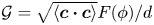 $\mathcal {G}=\sqrt {\langle \boldsymbol {c}\boldsymbol {\cdot }\boldsymbol {c}\rangle }F(\phi )/d$, where $F$ is a non-dimensional function of the volume fraction. This fluidity field is governed by an additional differential equation which is loosely based on the partial-fluidisation theory of Aranson & Tsimring (Reference Aranson and Tsimring2002) and shares structural similarity with the Ginzburg–Landau theory of phase transitions. As in the kinetic theory, at steady state the NGF model predicts smooth diffusion of the fluctuations, and as in Cosserat theory, a proposed length scale mediates the spatial variations.
The NGF theory was applied to steady vertical flow by Kamrin & Koval (Reference Kamrin and Koval2012) who used a pressure-controlled cell in which the fixed vertical direction was periodic and the bounding transverse walls moved dynamically to set a prescribed pressure. Coupled to the incompressible  $\mu (I)$-rheology, as detailed above in § 4.1, the non-local theory smoothed the transition between the shear regions and the plug and thus provided a good fit for DEM data. A recent extension to this is the work of Kim & Kamrin (Reference Kim and Kamrin2020) who detail collapses of both $\mu$ and $T_g$ against $\phi$ in the shear-plug transition region for vertical flow and a range of other geometries. Their proposed linear $\phi -\mu$ fit is similar to the laws here, which can be seen by combining (3.10) with (3.9) to give
 \begin{equation} \varPhi(\mu)=\phi_c-\frac{a}{b}(\mu-\mu_c) . \end{equation}
However, the parameter values are different as the fits in the present work account for the high- $I$ values close to the walls whereas Kim & Kamrin (Reference Kim and Kamrin2020) neglect these regions. This suggests that a nonlinear or piecewise curve could bridge the gap between these fits.
Liu & Henann (Reference Liu and Henann2018) also considered vertical chute flow as a test case for the NGF model. The focus of that paper being the isolation of the transition between fully static material and flowing material. This transition was found to occur when the channel is sufficiently wide, a finite-size effect that would not be present in the  $\mu (I)$, $\varPhi (I)$-rheology. It remains to be seen, however, how the non-local length scale affects the fully developed flow solutions and hence $\delta$.
5. Conclusions and discussion
The exact solutions derived here match the scaling behaviour of equivalent DEM simulations very well and even provide a good approximation to the spatial variation of the flow fields in both the cylindrical pipe and parallel-walled geometries. This success is despite the simplified nature of the linearised  $\mu (I)$, $\varPhi (I)$-rheology, which has enabled the exact solutions, and which means that certain complexities of the real flow are neglected. However, the direct link provided here to the realistic flow in a hopper-fed system hopefully ensures a broad range of applicability of the present model. Furthermore, the simplicity and veracity of these results suggests a universality that should be tested experimentally with real granular materials and in a range of geometries.
Whilst much novelty has been revealed by this study, particularly in the scaling of the shear zone, this does not necessarily rule out other theories, such as those detailed in § 4, which may indeed by more relevant for flows in distinctly different regimes, such as slow quasi-static deformations and in narrow pipes. There is also much scope for improving the handling of the interface with and flow in the approximate plug in the centre of the flow. This transition between inertial fluid-like and quasi-static solid-like flow is already the focus of extended theories, such as those proposed by Chialvo et al. (Reference Chialvo, Sun and Sundaresan2012) and Vescovi & Luding (Reference Vescovi and Luding2016), although they have not yet been applied to vertical chute flow. It is also evident in the flow field comparisons of figures 7 and 10 that the DEM velocities vary more smoothly than the current solutions, suggesting that the non-local extension of Kamrin & Koval (Reference Kamrin and Koval2012), in which diffusing fluctuations modify the flow, could improve these.
Other physically relevant extensions may also be made to account for the specifics of the bounding walls and for the particular granular material used in real systems. One aspect, that has been neglected here is the slip velocity observed along insufficiently frictional confining walls. It is well known that forming appropriate boundary conditions for this purpose is problematic (see Shojaaee et al. Reference Shojaaee, Roux, Chevoir and Wolf2012) and it may require additional closure equations, physical variables and extended DEM contact models to fully realise. Polydispersity of the grains has also been neglected here, but, as shown by Fan & Hill (Reference Fan and Hill2011), can invoke important feedbacks between the flow fields and distribution of material. A framework for handling this coupling has recently been proposed by Barker et al. (Reference Barker, Rauter, Maguire, Johnson and Gray2021) and capturing segregation in a vertical channel would be an important test case.
Whilst the approximations presented here are quasi-one-dimensional, the DEM geometries are all fully three-dimensional. This makes the fitting successes even more surprising as the  $\mu (I)$, $\varPhi (I)$-rheology has most commonly been justified using planar quasi-two-dimensional flow. This tendency is reflected in the studies of Rauter, Barker & Fellin (Reference Rauter, Barker and Fellin2020) and Baker et al. (Reference Baker, Guillard, Marks and Einav2018) who each found that granular flows in complex three-dimensional scenarios may reliably be approximated by planar flow fields. However, even with this reduced complexity, normal stress differences (see Alam et al. Reference Alam, Luding, Garcia-Rojo, Herrmann and McNamara2005) are apparent and are likely to be sensitive to the geometrical details, especially if the confining boundaries are not symmetric.
This paper has considered only steady solutions for this problem. However, as shown by Heyman et al. (Reference Heyman, Delannay, Tabuteau and Valance2017), the  $\mu (I)$, $\varPhi (I)$-rheology leads to ill-posed dynamic equations for transient flows. Alternative theories have been proposed recently by Barker et al. (Reference Barker, Schaeffer, Shearer and Gray2017) and by Schaeffer et al. (Reference Schaeffer, Barker, Tsuji, Gremaud, Shearer and Gray2019) which are instead made well posed via additional dependence on the dynamic compression and dilation of material. Given that the present work has established accurate steady solutions, a study of transient flows in pipes using these dynamic models would be of significant interest.
Supplementary movies
Supplementary movies are available at https://doi.org/10.1017/jfm.2021.909.
Acknowledgements
T.B. would like to thank Professor D. Schaeffer, Professor N. Gray and Dr D. Harris for inspiring discussions on this subject.
Funding
This work was supported by the Natural Environment Research Council (grant numbers NE/T010517/1, NE/R011001/1 and NE/W004240/1); the Engineering and Physical Sciences Research Council (grant number EP/N025318/1); The Royal Academy of Engineering/The Leverhulme Trust Senior Research Fellowship (grant number LTSRF1617/13/2); the National Natural Science Foundation of China (grant numbers 41831291, 51808401) and the China Postdoctoral Science Foundation (grant number 2020T130472).
Declaration of interests
The authors report no conflict of interest.
Author contributions
Both T.B. and C.Z. contributed equally to this work. T.B. was responsible for the theoretical aspects, C.Z. for the DEM computations and J.S., T.B. and C.Z. for the context, organisation and literature review.
Appendix A. Convenient coarse-graining formulae for one-dimensional flow fields
Many flows of interest have variation in only one spatial coordinate  $x$ that is normal to the flow direction $y$. As an alternative to first coarse graining the data in two or three dimensions, which is expensive, here a convenient formula is derived for directly evaluating one-dimensional variations. This follows Goldhirsch (Reference Goldhirsch2010) and Weinhart et al. (Reference Weinhart, Thornton, Luding and Bokhove2012) by replacing the spherical particles with smoothed functions $\mathcal {W}$. Continuum fields are then constructed from the sum over $N_p$ particles located at positions $\boldsymbol {r}_i=x_i\hat {\boldsymbol {x}}+y_i\hat {\boldsymbol {y}}+z_i\hat {\boldsymbol {z}}$ such as the volume fraction
 \begin{equation} \phi(\boldsymbol{r},t) = \sum_{i=1}^{N_p} V_i \mathcal{W}(\boldsymbol{r}-\boldsymbol{r}_i) , \end{equation}
where  $V_i={\rm \pi} d_i^3 /6$ is the volume of particle $i$. Instead of evaluating this for all $y$ and $z$, just the average in $0\leq y\leq L_y$ and $0\leq z\leq L_z$ is computed here i.e.
 \begin{equation} \langle \phi\rangle_{y,z} (x,t) = \frac{1}{L_y L_z} \sum_{i=1}^{N_p}V_{i} \int_0^{L_z}\int_0^{L_y} \mathcal {W}(\boldsymbol{r}-\boldsymbol{r}_i)\,\textrm{d} y \,\textrm{d}z. \end{equation}
Different choices of  $\mathcal {W}$ is possible, but here Gaussian kernels
 \begin{equation} \mathcal{W} =\frac{1}{c^3(2{\rm \pi})^{3/2}}\exp\left(-\frac{(x-x_i)^2+(y-y_i)^2+(z-z_i)^2}{2c^2}\right) , \end{equation}
where  $c$ is the coarse-graining width, will be used. Because these functions technically extend to infinity, some vanishingly small contribution will be lost when evaluating definite integrals. To limit this, $y_i=L_y/2\ \forall i$ and $z_i=L_z/2\ \forall i$ will be taken, in essence stacking all the particles in the middle $x$ plane far from the boundaries. Evaluating (A2) then gives
 \begin{equation} \langle \phi\rangle_{y,z} (x,t) = \text{erf}\left(\frac{L_y}{2\sqrt{2}c}\right) \text{erf}\left(\frac{L_z}{2\sqrt{2}c}\right) \frac{1}{\sqrt{2{\rm \pi}}c L_y L_z} \sum_{i=1}^{N_p}V_{i} \exp\left(-\frac{(x-x_i)^2}{2c^2}\right) , \end{equation}
for which the error functions tend to unity if  $c\ll L_y$ and $c\ll L_z$. If the $x\in [0,L_x]$ coordinate is also periodic, contributions from $x<0$ and $x>L_x$ need to be shifted accordingly, as was done for the fully periodic simulations. The other fields of interest, such as the velocity
 \begin{equation} \langle \boldsymbol{u}\rangle _{y,z} (x,t) \simeq \frac{1}{\sqrt{2{\rm \pi}}c L_y L_z \langle \phi\rangle_{y,z}} \sum_{i=1}^{N_p}V_{i} \boldsymbol{u}_i \exp\left(-\frac{(x-x_i)^2}{2c^2}\right) , \end{equation}
may also be easily computed using this procedure.
Appendix B. Stress calculation and the $\mu (I)$ and $\varPhi (I)$ relations


In order to calculate the pressure  $p$ and shear stress $\tau$, which are required to for estimating $\mu$ and $I$, the full stress tensor $\boldsymbol {\sigma }$ is first computed. This calculation necessarily involves fully three-dimensional considerations, so a simplified one-dimensional treatment, like that of Appendix A, is not easily achieved. Instead we first calculate the stress components for all particles within each cubic sample volume $V=d^3$ before averaging. The stress is composed of contributions from contacts as well as from the kinetic motion of the grains and is defined for each volume as
 \begin{equation} \boldsymbol{\sigma} =\frac{1}{V} \sum_{\forall i\in V} \left[\sum_{\forall j\neq i\in V}\boldsymbol{r}_{ij}\boldsymbol{F}_{ij} + m(\boldsymbol{u}_i-\bar{\boldsymbol{u}})^2\right], \end{equation}
where  $\boldsymbol {r}_{ij}$ and $\boldsymbol {F}_{ij}$ are the pair centre-to-centre vector and force respectively, $m=\rho _*{\rm \pi} d^3/6$ is the grain mass and $\bar {\boldsymbol {u}}$ is the mean velocity of the sample. Given this, the pressure and non-zero shear stress are
 \begin{equation} p={-}\tfrac{1}{3}\mathrm{Tr}(\boldsymbol{\sigma}), \quad \text{and} \quad \tau_{xz}=\sigma_{xz}. \end{equation}
Figure 13 shows how the stress ratio  $\mu =\tau _{xz}/p$ and solid volume fraction $\phi$ vary with the inertial number $I$, which is defined in (3.5). Here, data are collated for each of the different geometries and for a range of different control parameters. At intermediate values of $I$ both plots show a universal collapse, indicating that the $\mu (I)$, $\varPhi (I)$-rheology is a good description in the shear zones. As expected, the collapse is not so good in the plug, where $I$ is small, and additional physics come into play. In addition to the non-inertial flow behaviour, the plots show some nonlinearity, even in the shear zones. However, inclusion of these effects in the analysis of § 3 would obscure the clarity achieved by the leading-order behaviour, which is well approximated by the linear functions.

Figure 13. Steady-state rheology extracted from DEM simulations of differing pipe width  $W$. Panel $(a)$ shows the bulk friction $\mu$ and $(b)$ is the solid volume fraction $\phi$ as functions of the inertial number $I$. Squares are from the doubly wide periodic cells and circles are for the cylindrical pipe simulations. These cases all have $\phi _0=0.56$ whereas additional cases with $W=150d$ and $\phi _0=0.5$ and $\phi _0=0.6$ are plotted as upward $\triangle$ and downward $\triangledown$ triangles,respectively. Solid lines are the linear $\mu (I)$ and $\varPhi (I)$ functions given in (3.10) and (3.9) respectively with parameters found in table 2. Inset in each panel are the same data but plotted on a linear, rather than logarithmic, scale for the horizontal axis.


 Open access