


1. Introduction
Turbulent boundary layers subjected to an adverse pressure gradient still pose many open questions. At the same time, they have a high relevance in many technical applications, e.g. airplane wings, turbomachinery blades and wind turbine blades. Here, the flows around airplane wings are special due to the very high Reynolds numbers (Re). The proper mathematical description of the statistically averaged mean flow of a turbulent boundary layer at a significant adverse pressure gradient (APG) is still under debate. For boundary layers at zero pressure gradient (ZPG), there is large experimental support and agreement in the literature that, for sufficiently large Reynolds numbers, the mean velocity in a large part of the inner layer can be described by the log law
 \begin{equation} u^{+}=\frac{1}{\kappa}\log(y^{+})+B, \end{equation}
see e.g. Marusic et al. (Reference Marusic, Monty, Hultmark and Smits2013). The superscript  $+$ denotes viscous units. For the von Kármán constant $\kappa$ and for the intercept $B$, Österlund et al. (Reference Österlund, Johansson, Nagib and Hites2000) found $\kappa =0.384$ and $B=4.17$, compared to $\kappa =0.41$ and $B=5.0$ by Coles & Hirst (Reference Coles and Hirst1969).
The results for the structure of the mean-velocity profile for turbulent boundary layers at ZPG are supposed to give guidance for the APG case. Traditionally, the boundary layer is divided into four layers, i.e. the viscous sublayer ( $y^{+}<5$), the buffer layer $(5<y^{+}<30$), the logarithmic layer ( $30<y^{+}<0.15\delta ^{+}$) and the wake layer ( $y^{+}>0.15\delta ^{+}$), where $\delta$ denotes the boundary layer thickness, see e.g. Wei et al. (Reference Wei, Fife, Klewicki and McMurtry2005) for a review. Recent publications indicate agreement on the outer edge of the log layer near $y=0.15\delta$, see Marusic et al. (Reference Marusic, Monty, Hultmark and Smits2013). The extent of the log law in terms of $\delta$ depends on the method to determine $\delta$. Marusic et al. (Reference Marusic, Monty, Hultmark and Smits2013) determined $\delta$ from a fit of the composite law of the wall/law of the wake, and $\delta$ defined in this way is approximately $25\,\%$ to $35\,\%$ larger than $\delta _{99}$, see e.g. Marusic et al. (Reference Marusic, Chauhan, Kulandaivelu and Hutchins2015). The region $y<0.15\delta$ will be referred to as the inner layer. Regarding the beginning of the log layer, larger values ranging from $y^{+}>150$ up to $y^{+}>300$ have been proposed recently. A mesolayer located between the buffer layer and the log layer, first proposed by Long & Chen (Reference Long and Chen1981) and Afzal (Reference Afzal1982), was associated with the region $30<y^{+}<300$ in George & Castillo (Reference George and Castillo1997). Another view was given by Marusic et al. (Reference Marusic, Monty, Hultmark and Smits2013), who found at very high Reynolds numbers the existence of a region where the log law for the mean velocity and a logarithmic profile for the streamwise (and spanwise) turbulence intensities hold simultaneously, leading to $3\textit {Re}_\tau ^{1/2} < y^{+}<0.15 \textit {Re}_\tau$ for the log-law region. An alternative view was given by Wei et al. (Reference Wei, Fife, Klewicki and McMurtry2005) based on a study of the mean momentum balance in differential form. Their log-law region IV is where the mean viscous force loses leading-order influence, and begins at $y^{+}=2.6\textit {Re}_\tau ^{1/2}$, see Klewicki, Fife & Wei (Reference Klewicki, Fife and Wei2009).
For flows with a significant APG, the discussion described in Alving & Fernholz (Reference Alving and Fernholz1995) is still open. A first hypothesis is that the log law (1.1) still holds and that  $\kappa$ and $B$ still have the same values as for a turbulent boundary layer at ZPG, but that the region occupied by the log law is progressively reduced with increasing APG. This hypothesis was called the ‘progressive breakdown’ of the law of the wall in Galbraith, Sjolander & Head (Reference Galbraith, Sjolander and Head1977), and was advocated for by, among others, Coles (Reference Coles1956), Perry (Reference Perry1966) and Coles & Hirst (Reference Coles and Hirst1969).
In conjunction with the first hypothesis, Perry, Bell & Joubert (Reference Perry, Bell and Joubert1966) proposed that above the log-law region a so-called half-power-law region arises. In the special case of a vanishing wall shear stress close to separation, the half-power law extends almost down to the wall. This proposal by Stratford (Reference Stratford1959) was recently supported by direct numerical simulations in Coleman et al. (Reference Coleman, Pirozzoli, Quadrio and Spalart2017) and Coleman, Rumsey & Spalart (Reference Coleman, Rumsey and Spalart2018). Modified versions of this wall law are given in Kader & Yaglom (Reference Kader and Yaglom1978) and in Afzal (Reference Afzal2008).
A second hypothesis is that the coefficients  $\kappa$ and $B$ of the log law change their values. A functional dependence of $\kappa$ on the pressure gradient parameter in inner scaling $\Delta p_s^{+}$
 \begin{equation} \Delta p_s^{+}=\frac{\nu}{\rho u_\tau^{3}}\frac{\mathrm{d}P_{w}}{\mathrm{d}s} \end{equation}
was proposed by Nickels (Reference Nickels2004), where  $\mathrm {d}P_{w}/\mathrm {d}s$ denotes the pressure gradient at the wall in the wall-parallel direction, p pressure, $\nu$ kinematic viscosity and $\rho$ density. An alternative relation was given by Dixit & Ramesh (Reference Dixit and Ramesh2009). To illustrate the extent of variability of $\kappa$, the model by Nickels (Reference Nickels2004) predicts a reduction from $\kappa =0.390$ at ZPG to $\kappa =0.370$ for $\Delta p_s^{+}=0.01$ at APG. For increasing $\Delta p_s^{+}$, the model predicts $\kappa =0.353$ for $\Delta p_s^{+}=0.02$, and $\kappa =0.329$ for $\Delta p_s^{+}=0.04$. The model by Dixit & Ramesh (Reference Dixit and Ramesh2009) predicts a faster reduction from $\kappa =0.408$ at ZPG to $\kappa =0.376$ for $\Delta p_s^{+}=0.01$, $\kappa =0.346$ for $\Delta p_s^{+}=0.02$ and $\kappa =0.293$ for $\Delta p_s^{+}=0.04$. Therefore, experimental support for the hypothesis of a variability of $\kappa$ is supposed to require values of $\Delta p_s^{+}>0.01$. Regarding a possible change of $\kappa$ and $B$, a number of data sets were evaluated by Monkewitz, Chauhan & Nagib (Reference Monkewitz, Chauhan and Nagib2008), who found an empirical correlation between $\kappa$ and $B$. Experimental results by Nagano, Tagawa & Tsuji (Reference Nagano, Tagawa and Tsuji1991) could indicate a change in $B$, and the direct numerical simulation (DNS) data by Lee & Sung (Reference Lee and Sung2009) give indications that $\kappa$ and $B$ may change.
A third hypothesis is that the pressure gradient causes ‘[…] a change in the character of the velocity distribution over the entire region […]’ occupied by the log law in a ZPG flow, see Galbraith et al. (Reference Galbraith, Sjolander and Head1977), called a ‘general breakdown’ of the log law. Some authors proposed a single formulation for the entire inner layer based on the half-power law (or square-root law, abbreviated: sqrt-law), see Townsend (Reference Townsend1961)
 \begin{align} u^{+}=\frac{1}{K_{o}}\left[\log(y^{+}) +2\left(\sqrt{1+\Delta p_s^{+} y^{+}}-1\right) +2\log\left( \frac{2}{\sqrt{1+\Delta p_s^{+} y^{+}}+1}\right)\right] + B_{o}. \end{align}
In the theoretical analysis, the half-power law is assumed to be associated with the total shear stress growing linearly with the wall distance, see e.g. Brown & Joubert (Reference Brown and Joubert1969).
In this work, the analysis of a new turbulent boundary layer experiment is presented, whose aim was to answer the following questions for the mean velocity profile:
(Q1) Does a log-law region still exist at APG?
(Q2) Does the von Kármán constant $\kappa$ change with $\Delta p_s^{+}$, see Nickels (Reference Nickels2004)?
(Q3) Is there a sqrt-law region above the log law, see e.g. Perry et al. (Reference Perry, Bell and Joubert1966)?


These questions were motivated by a literature study and by the results of the precursor experiment by Knopp et al. (Reference Knopp, Schanz, Schröder, Dumitra, Hain and Kähler2014b). Therein, a turbulent boundary layer was studied, where the flow followed an  $S$-shaped deflection of the geometry model, which caused a strong APG up to $\Delta p_s^{+}=0.06$ and $\textit {Re}_\theta$ up to $18\,000$, see figure 2 in Knopp et al. (Reference Knopp, Schanz, Schröder, Buchmann, Cierpka, Hain and Kähler2014a). A three-layer form for the mean velocity as described by Perry et al. (Reference Perry, Bell and Joubert1966) was found, see figure 3 in Knopp et al. (Reference Knopp, Schanz, Schröder, Buchmann, Cierpka, Hain and Kähler2014a). A small log-law region was indicated from a thin plateau of the slope diagnostic function, see figure 5 in Knopp et al. (Reference Knopp, Schanz, Schröder, Buchmann, Cierpka, Hain and Kähler2014a), and $\kappa$ was found to be reduced in the APG region, see figure 6 in Knopp et al. (Reference Knopp, Schanz, Schröder, Dumitra, Hain and Kähler2014b). A half-power law was observed above the log law, albeit only over a small region in terms of $y^{+}$. The question arose as to whether a higher $\textit {Re}$ leads to a larger extent of the log law and of the half-power-law region.
Several new experiments and numerical simulations for turbulent boundary layers at APG have been provided during the last decade. Wind-tunnel experiments were performed by, e.g. Atkinson et al. (Reference Atkinson, Buchner, Eisfelder, Kitsios and Soria2016), Monty, Harun & Marusic (Reference Monty, Harun and Marusic2011), Harun et al. (Reference Harun, Monty, Mathis and Marusic2013) and Schatzman & Thomas (Reference Schatzman and Thomas2017). New numerical simulations were accomplished by, e.g. Lee & Sung (Reference Lee and Sung2009), Gungor et al. (Reference Gungor, Maciel, Simens and Soria2016), Coleman et al. (Reference Coleman, Pirozzoli, Quadrio and Spalart2017) and Coleman et al. (Reference Coleman, Rumsey and Spalart2018). Regarding the mean flow and the turbulence statistics, most of the work focussed on the outer part of the boundary layer, whereas the inner layer was studied in detail only in Coleman et al. (Reference Coleman, Pirozzoli, Quadrio and Spalart2017) and in Coleman et al. (Reference Coleman, Rumsey and Spalart2018).
Flow experiments with pressure gradients and streamwise surface curvature are rare in the literature, see Baskaran, Smits & Joubert (Reference Baskaran, Smits and Joubert1987) and Bandyopadhyay & Ahmed (Reference Bandyopadhyay and Ahmed1993). Flows with surface curvature alone have been studied in depth since the work by Bradshaw (Reference Bradshaw1970). For the present work, convex curvature is relevant. The magnitude of curvature effects depends on the ratio of the local boundary layer thickness  $\delta$ to the local radius of curvature $R_c$. Large curvature effects are associated with values for $\delta /R_c>0.05$, see e.g. Gillis & Johnston (Reference Gillis and Johnston1983). Values of $\delta /R_c<0.01$ are associated with mild curvature, which were studied e.g. by Ramaprian & Shivaprasad (Reference Ramaprian and Shivaprasad1978). The relaxation of a turbulent boundary layer from curvature on a flat plate was studied for the ZPG case by Gillis & Johnston (Reference Gillis and Johnston1983) and by Alving, Smits & Watmuff (Reference Alving, Smits and Watmuff1990).
The focus of the present work is on the behaviour of the mean-velocity profile, and we only use the single-point statistics. In complementary publications the simultaneous spatial information provided by the 2D2C data, i.e. planar data (two-dimensional) of two components (2C) of the velocity, and 3D3C data, i.e. volumetric data for all three components (3C) of the velocity were exploited. The characterisation of coherent structures is described in Reuther et al. (Reference Reuther, Scharnowski, Hain, Schanz, Schröder and Kähler2015) and Reuther (Reference Reuther2019). The interaction of coherent flow structures is studied in Bross, Fuchs & Kähler (Reference Bross, Fuchs and Kähler2019). Their representation using the attached eddy model is described in Eich et al. (Reference Eich, de Silva, Marusic and Kähler2020), and the intermittent behaviour is analysed in Reuther & Kähler (Reference Reuther and Kähler2018), Reuther (Reference Reuther2019) and Reuther & Kähler (Reference Reuther and Kähler2020).
This paper is organised as follows. The wind-tunnel experiment is described in § 2. The description of the flow is given in § 3. The central part is formed by the results in the APG region and their analysis in § 4. In § 5, history effects in the inner and outer layers are discussed. The conclusions of the analysis are summarised in § 6.
2. Experimental investigation
The aim of the experiment was to answer the three questions formulated in the introduction. Regarding the hypothesis by Nickels (Reference Nickels2004), (A7) was used to estimate the supposed change of  $\kappa$. This led to the first design condition (C1) to reach $\Delta p_s^{+}>0.01$ in the focus region of the APG, so that a possible change of $\kappa$ due to the pressure gradient is large enough to be distinguished from uncertainties related to the evaluation of $\kappa$ and the determination of $u_\tau$. For this purpose, the measurements were performed on the contour geometry model and not on the flat wind-tunnel wall opposite to the model, since the values of $\Delta p_s^{+}$ are significantly larger on the contour model. The second design condition (C2) was to reach large Reynolds numbers in the APG focus region, based on the assumption that only at large Reynolds numbers does the asymptotic structure of the wall law with significantly thick log-law and sqrt-law regions form.
Two additional conditions were a consequence of the aim to use the measurement technique as accurate as possible. The third condition (C3) was to use a flat surface in the APG focus region to enable measurements through a glass plate from behind to reduce the issue of reflections of particle imaging methods in the near-wall region. The fourth design condition (C4) was to achieve large Reynolds numbers at moderately low flow speeds and large boundary layer thicknesses to enable accurate measurements in the viscous sublayer. Due to the design condition (C4) in conjunction with the decision to measure on the geometry model, the issue of surface curvature effects arose. We accepted this issue. The option was to reach  $\Delta p_s^{+}>0.01$ on the wind-tunnel wall and a much stronger pressure gradient on the geometry model, causing the flow to separate. This idea was abandoned, since it would have meant to either accept a three-dimensional separation or to use flow actuation to prevent separation. The latter was not pursued due to the technical challenges to achieve well-defined and reproducible flow conditions.
2.1. Design of the experiment and set-up in the wind tunnel
The experiment was performed in the Eiffel type atmospheric wind tunnel of UniBw in Munich, which has a  $22$ m long test section with a rectangular cross-section of $2\ \mathrm {m}\times 2\ \mathrm {m}$. As described in figure 1, the flow develops on the sidewall of the wind tunnel over around $4\ \mathrm {m}$ and is then accelerated along a first ramp of height $0.30\ \mathrm {m}$ and of length $1.225\ \mathrm {m}$. Then, the flow gradually develops along a flat plate of length $4.0\ \mathrm {m}$ with ZPG into an equilibrium. The flow follows a curvilinear deflection of length $l_c=0.75\ \mathrm {m}$ which initially causes a small favourable pressure gradient (FPG), and enters into the APG region. The focus region is an inclined flat plate of length $0.4\ \mathrm {m}$, beginning at $x=9.75\ \mathrm {m}$, at an opening angle of $\alpha =14.4^{\circ }$ with respect to the $4.0\ \mathrm {m}$ long flat plate. Finally, the flow follows a second deflection down to the wind-tunnel wall. The opening angle was chosen to keep the flow remote from separation in a more conservative way than in the precursor experiment by Knopp et al. (Reference Knopp, Schanz, Schröder, Dumitra, Hain and Kähler2014b) and was designed based on computational fluid dynamics (CFD) results with the DLR TAU code using the Spalart–Allmaras model and the shear stress transport (SST) $k$-
$k$- $\omega$ model, where k is turbulent kinetic energy and $\omega$ is specific dissipation rate.

Figure 1. Sketch of the wind-tunnel experiment with flow direction (axes not to scale).
The coordinate system shown in figure 1 denotes by  $x$ the direction parallel to the floor of the wind tunnel. The origin $x=0$ is defined at the nominal beginning of the test section, which is located $0.875\ \mathrm {m}$ downstream of the thinnest cross-section of the contraction. The curvilinear deflection can be described by a fourth-order polynomial $f(\zeta )$. Here, $\zeta$ denotes the relative coordinate $\zeta =x-8.99\ \mathrm {m}$, i.e. $\zeta =0$ at the beginning of the curvilinear element and $\zeta =l_c$ at its end. Then the conditions of a smooth transition between the flat plate and the curved wall imply $f'(0)=0$, $f'(l_c)=a=\arctan ({\rm \pi} \alpha /180)$ with $\alpha =14.4^{\circ }$, and $f''(0)=f''(l_c)=0$, where $f'$ and $f''$ denote the first and second derivatives. This leads to $f(\zeta )=-a/(2l_c^{3})\zeta ^{4}+a/l_c^{2} \zeta ^{3}$. In order to reduce the effects of the sidewalls, the dimension of the APG part of the geometry was reduced by a factor of two compared to the previous experiment by Knopp et al. (Reference Knopp, Schanz, Schröder, Dumitra, Hain and Kähler2014b).
The experimental results presented here were performed at a free-stream velocity  $U_\infty =23\ \mathrm {m}\ \mathrm {s}^{-1}$ and $U_\infty =36\ \mathrm {m}\ \mathrm {s}^{-1}$, measured at a reference position near the beginning of the test section. The values for $\textit {Re}_\theta$ of 24 400 and 35 900 at $x=8.12\ \mathrm {m}$ (ZPG region) respectively 40 000 and 57 400 at $x=9.944\ \mathrm {m}$ (APG region) are among the highest after the experiments in Coles & Hirst (Reference Coles and Hirst1969), and comparable to those of Skare & Krogstad (Reference Skare and Krogstad1994) and Nagib, Christophorou & Monkewitz (Reference Nagib, Christophorou and Monkewitz2004). The static pressure measurements were performed using two DTC Initium Systems, where 64 channels were used in parallel, in the centreline and in different spanwise planes. The free-stream turbulence intensity (FSTI) was quantified in the empty test section in Schulze (Reference Schulze2012). The mean FSTI was $0.14\,\%$ measured at $x=2.5\ \mathrm {m}$ for $U_\infty =38\ \mathrm {m}\ \mathrm {s}^{-1}$, averaged over the entire cross-section. The FSTI variation was found to be between $0.10\,\%$ and up to $0.19\,\%$ towards the corners. The variation of the FSTI was not measured in the flow direction for the wind tunnel with the contour model. Therefore, a possible influence on the boundary layer could not be assessed.
2.2. Measurement technique
Different particle imaging approaches were combined in order to measure the mean velocity and the Reynolds stresses over a streamwise extent of several boundary layer thicknesses from the outer edge of the boundary layer down to the viscous sublayer.
2.2.1. Large-scale 2D2C particle image velocimetry
For an overview measurement from  $x=8\ \mathrm {m}$ to $x=10.2\ \mathrm {m}$ a multi-camera large-scale 2D2C-particle image velocimetry (PIV) measurement was applied using 9 cameras, named c1 to c9. The cameras c1 to c7 were located in the region of ZPG, FPG and mild APG, whereas the cameras c8 and c9 were located in the region of the largest APG. The 2D2C-PIV data were evaluated using a single-pixel ensemble correlation and a window correlation method, see Reuther et al. (Reference Reuther, Scharnowski, Hain, Schanz, Schröder and Kähler2015). The interrogation window (IW) size was $16\ \mathrm {px}\times 16\ \mathrm {px}$ and the interrogation step size was $8 \ \mathrm {px}$, corresponding to an overlap of $50\,\%$. From the 2D2C-PIV data, the mean-velocity profiles were extracted at 13 selected streamwise positions. Details of the PIV method are given in table 1.
Table 1. Summary of the experimental parameters for the reference position  $x_{ref}=9.944\ \mathrm {m}$. The flow was seeded with DEHS droplets with a diameter of approx. $1\ \mathrm {\mu }\mathrm {m}$. px, pixel.

The spatial resolution of the PIV method depends mainly on the magnification of the imaging system, the pixel size of the recording cameras and the selected IW dimensions, see Kähler, Scharnowski & Cierpka (Reference Kähler, Scharnowski and Cierpka2012a). To locally capture the entire boundary layer, the nine sCMOS cameras were equipped with  $50\ \mathrm {mm}$ Zeiss lenses (c1–c7) and $35\ \mathrm {mm}$ Zeiss lenses (c8–c9), respectively. In the regions of ZPG, FPG and mild APG, the field of view was $0.32\ \mathrm {m}\times 0.27\ \mathrm {m}$ and the interrogation volume size was $2\ \mathrm {mm}\times 2\ \mathrm {mm}\times 1\ \mathrm {mm}$ yielding a resolution of $8\ \mathrm {px}\ \mathrm {mm}^{-1}$ for cameras c1 to c7. Regarding the resolution in viscous units $\delta _\nu$ at $x=8.12\ \mathrm {m}$, the IW size was $l_y^{+}=125$ based on $\delta _\nu =\nu /u_\tau =16\ \mathrm {\mu } \mathrm {m}$ for $U_\infty =23\ \mathrm {m}\ \mathrm {s}^{-1}$. In the APG region the field of view was $0.44\ \mathrm {m}\times 0.37\ \mathrm {m}$ and the interrogation volume $l_x\times l_y\times l_z$ was $2.7\ \mathrm {mm}\times 2.7\times 1\ \mathrm {mm}$. The IW size in the wall-normal direction was $l_y^{+}=91$ for camera c8 at $x_{ref}=9.944\ \mathrm {m}$.
2.2.2. Particle tracking velocimetry
To resolve the near-wall region, a high magnification approach using long-range microscopic particle tracking velocimetry (2D- ${\mu }$PTV), see Kähler, Scharnowski & Cierpka (Reference Kähler, Scharnowski and Cierpka2012b), was applied at the position $x_{ref}=9.944\ \mathrm {m}$ in the APG region. The wall-normal extent of the field of view was $140\delta _\nu$ for the case $U_\infty =23\ \mathrm {m}\ \mathrm {s}^{-1}$. The size of a bin in the wall-normal direction was $0.27\delta _\nu$.
The three-dimensional Lagrangian particle tracking (LPT) approach using the shake-the-box (STB) method was used for the case  $U_\infty =36\ \mathrm {m}\ \mathrm {s}^{-1}$, see Novara et al. (Reference Novara, Schanz, Reuther, Kähler and Schröder2016). The macroscopic field of view of $50\ \mathrm {mm} \times 90\ \mathrm {mm} \times 8$ covered approximately $0.4\delta _{99}$. In this work we use the data which were sampled over a bin size of $2.88\delta _\nu$ in the wall-normal direction. This evaluation will be referred to as LPT detail.
For a study of the terms of the mean momentum equation, a second evaluation was performed. The field of view was divided into 111 bins in the wall-normal direction and 5 bins in the wall-parallel direction, corresponding to a bin size of  $321\ \mathrm {px}\times 30\ \mathrm {px}$ (or $9.2\ \mathrm {mm} \times 0.86\ \mathrm {mm}$) in the streamwise and wall-normal directions. The gradients were evaluated using a linear interpolation over a kernel of 5 points located in the centre of each bin. The choice of the large bin size in streamwise direction was motivated by statistical convergence reasons, as more than 400 000 entries per bin are available to estimate the mean and fluctuating velocity components. Since the bin size in wall-normal direction corresponds to around $41\delta _\nu$, this evaluation is referred to as LPT average (abbreviated LPT ave).
2.2.3. Oil-film interferometry
The wall shear stress was measured using oil-film interferometry (OFI) from  $x=8.33\ \mathrm {m}$ to $x=10.02\ \mathrm {m}$. This provides absolute measurements of the wall shear stress independent of any assumption on the mean-velocity profile. The uncertainty of the OFI measurement technique for determining the average friction velocity was estimated to be smaller than $2\,\%$ (with a $95\,\%$ confidence level) based on Thibault & Poitras (Reference Thibault and Poitras2017). For technical details of the oil-film interferometry measurements we refer to Schülein, Reuther & Knopp (Reference Schülein, Reuther and Knopp2017). The experiments using the different measurement techniques were performed at different days, nominally for the same values of $U_\infty$, see table 8 in appendix B. It was not possible to repeat the OFI measurements to obtain the same Reynolds numbers, since the contour model was deployed shortly after the measurement campaign.
3. Description of the flow
The flow and its streamwise evolution are described using the overview measurement. The aim is to show that the experimental set-up provides the intended flow conditions in the APG region. The set-up leads to a streamwise changing pressure gradient and convex surface curvature effects, which are also described.
3.1. Streamwise evolution of boundary layer parameters
The streamwise distribution of the pressure coefficient  $c_{{p}}$ is shown in figure 2(a). Moreover, ${\rm d}c_{{p}}/{\rm d}s$ is shown, where $s$ is the coordinate direction tangential to the contour wall. Note that $U_{ref}=U_\infty$ was used for the non-dimensionalisation of $c_{{p}}=(p-p_{ref})/q_{ref}$, with $q_{ref}=\rho _{ref} U_{ref}^{2}/2$. The streamwise distribution of $c_{{f}}=\tau _{w}/q_{ref}$ from OFI is shown in figure 2(b) for $U_\infty =23\ \mathrm {m}\ \mathrm {s}^{-1}$. Therein, $U_{ref}=U_{e}$ at $x=8.12\ \mathrm {m}$ is used for non-dimensionalisation. In the focus region at $x=9.944\ \mathrm {m}$ the flow is not close to separation. Downstream of $x=10.0\ \mathrm {m}$, the flow remains attached with $c_{f}$ significantly larger than zero, as inferred from the 2D2C PIV data. There were no indications for corner flow separation in the junction of the contour model and the wind-tunnel sidewall from tuft flow visualisation.

Figure 2. Streamwise distribution of  $c_{p}$ and ${\rm d} c_{p}/{\rm d}s$ (a) and $c_{f}$ from OFI (b) for $U_\infty =23\ \mathrm {m}\ \mathrm {s}^{-1}$.
The boundary layer thickness was evaluated using different methods, see figure 3(a). The conventional definition  $\delta _{99}$ and $\delta _{995}$ for a flat plate at ZPG uses the wall distance where the wall-parallel velocity reaches $99\,\%$ and $99.5\,\%$ of its maximum value along a wall-normal line. The maximum value could be determined for all profiles in the region $8\ \mathrm {m}<x<10.2\ \mathrm {m}$. On the curved wall, the profiles show a distinct maximum. On the flat wall in the APG region, $\partial U/\partial y$ becomes zero when approaching the boundary layer edge, see figure 3(b). Appendix C describes the other criteria used based on the generalised velocity $\tilde {U}$ by Coleman et al. (Reference Coleman, Rumsey and Spalart2018), which is shown in figure 3(b), on $u'/U$ by Vinuesa et al. (Reference Vinuesa, Bobke, Örlü and Schlatter2016), on the potential velocity $U_p$ for curved walls by Patel & Sotiropoulos (Reference Patel and Sotiropoulos1997) and on the turbulent/non-turbulent interface (TNTI) by Reuther & Kähler (Reference Reuther and Kähler2018). The values for $\delta _{99}$ are found to be in close agreement with the different proposals, and are therefore used to describe the boundary layer thickness in the following.

Figure 3. (a) Streamwise distribution of the boundary layer thickness evaluated using different criteria: U-tilde:  $\tilde {U}$ by Coleman et al. (Reference Coleman, Rumsey and Spalart2018); $u'/U$: by Vinuesa et al. (Reference Vinuesa, Bobke, Örlü and Schlatter2016); $U_p$: by Patel & Sotiropoulos (Reference Patel and Sotiropoulos1997); TNTI, $\gamma =0.3$: by Reuther & Kähler (Reference Reuther and Kähler2018). (b) Mean velocity profile for $U$,
$U$,  $\tilde {U}$ and $U_{p}$ at the ZPG position $x=8.12\ \mathrm {m}$, at $x=9.42\ \mathrm {m}$ on the curved wall at APG, and at $10.02\ \mathrm {m}$ on the inclined flat wall element at APG for $U_\infty =23\ \mathrm {m}\ \mathrm {s}^{-1}$.
The pressure gradient along the contour model is shown in terms of  $\Delta p_s^{+}$ in figure 4(a) and the Clauser–Rotta scaling $\beta _{RC}=\delta ^{*}/(\rho u_\tau ^{2})\,\mathrm {d}P_{w}/\mathrm {d}s$ in figure 4(b). Both become large in the APG region where $u_\tau$ becomes small. The pressure gradient parameter $\beta _{ZS}=\delta _{99}^{2}/(\rho U_{e}^{2} \delta ^{*})\,\mathrm {d}P_{w}/\mathrm {d}s$ in the scaling by Zagarola & Smits (Reference Zagarola and Smits1997) and Gungor et al. (Reference Gungor, Maciel, Simens and Soria2016), which does not involve $u_\tau$, is shown in figure 4(c). Downstream of the ZPG region, $\beta _{ZS}$ shows significant negative values for the FPG near $x=9.05\ \mathrm {m}$, then changes its sign and reaches large positive values with a maximum near $x=9.62\ \mathrm {m}$ near the maximum of $\mathrm {d}c_p/\mathrm {d}s$. The shape factor $H_{12}$ is shown in figure 5(a). The local ratio of the boundary layer thickness $\delta _{99}$ to the radius of curvature $R_c$ is shown in figure 5(b). The values for $\delta _{99}/R_c$ are larger than the value of $0.01$ which is associated with mild curvature in the literature. On the other hand, the value for $\delta ^{*}/R_c$ is smaller than $0.005$, which is lower by one order of magnitude than the criterion by Bradshaw (Reference Bradshaw1970) for strong curvature. The boundary layer parameters are summarised in table 2 for the 2D2C PIV measurements evaluated by the single-pixel method.

Figure 4. Streamwise pressure gradient parameter (a) in inner scaling, (b) in Clauser–Rotta scaling and (c) in the scaling by Zagarola & Smits for  $U_\infty =23\ \mathrm {m}\ \mathrm {s}^{-1}$.

Figure 5. (a) Shape factor  $H_{12}$ and (b) $\delta _{99}/R_c$ for $U_\infty =23\ \mathrm {m}\ \mathrm {s}^{-1}$ (geometry not to scale), and (c) eddy turnover length $\delta _{{t.o.}}$ for $U_\infty =36\ \mathrm {m}\ \mathrm {s}^{-1}$.
Table 2. Characteristic boundary layer parameters for the 2D2C PIV measurements evaluated by the PIV single-pixel ensemble correlation method.

The streamwise distance over which the pressure gradient changes may be compared to the boundary layer reference thickness, which is  $\delta _{99,{ref}}=0.15\ \mathrm {m}$ at $x=8.12\ \mathrm {m}$. The curvature first causes an FPG from $x=8.85\ \mathrm {m}$ to $x = 9.24\ \mathrm {m}$ over a streamwise length of $2.6\delta _{99,{ref}}$. The change of $\beta _{ZS}$ from a significant FPG to a significant APG from $x=9.05\ \mathrm {m}$ to $x = 9.62\ \mathrm {m}$ corresponds to $4\delta _{99,{ref}}$. In the APG region on the inclined flat plate for $x > 9.75\ \mathrm {m}$, the curvature is absent and $\beta _{ZS}$ is slowly decreasing in the streamwise direction. The focus measurement position at $x=9.944\ \mathrm {m}$ in the APG region is located $1.3\delta _{99,{ref}}$ downstream of the end of curvature. For more insight, the local boundary layer thickness is related to the eddy turnover length and to the large-scale coherence.
The eddy turnover length  $\delta _{{t.o.}}=U\tau _{t.o.}$ is the streamwise travelling distance of the local mean flow $U(y)$ corresponding to the eddy turnover time $\tau _{t.o.}$, see Sillero, Jimenez & Moser (Reference Sillero, Jimenez and Moser2013). Following this work, we assume that the flow relaxes to equilibrium within $2\tau _{t.o.}$. We compute $\tau _{t.o.}$ using the relation $\tau _{t.o.}=\kappa y / u^{*}$, where two options were used for the turbulent velocity scale $u^{*}$, i.e. $u^{*}=|\overline {u'v'}|^{1/2}$ and $u^{*}=k^{1/2}$ based on the turbulent kinetic energy $k$. In the APG region at $x=9.944\ \mathrm {m}$, we observe $2\delta _{t.o.}=0.5\delta _{99}$ for $u^{*}=k^{1/2}$ and $2\delta _{t.o.}=1.1\delta _{99}$ for $u^{*}=|\overline {u'v'}|^{1/2}$ at $y=0.1\delta _{99}$, see figure 5(c). This is seen as an indication that the near-wall flow relaxes rapidly, but not instantaneously. In the outer part of the boundary layer, the turnover length becomes larger. At $y/\delta _{99}=0.5$ we observe $2\delta _{t.o.}=22 \delta _{99}$ (based on $|\overline {u'v'}|$) and $2\delta _{t.o.}=7 \delta _{99}$ (based on $k$).
$k$).
An alternative streamwise length scale is the large-scale coherence in the flow. The largest values for the length scale from the two-point correlation map  $L_2$ were found at the wall distance $y=0.2\delta _{99}$ with $L_2=4\delta _{99}$ at $x=8.34\ \mathrm {m}$ (ZPG), $L_2=4\delta _{99}$ at $x=9.14\ \mathrm {m}$ (FPG) and $L_2=2\delta _{99}$ at $x=9.94\ \mathrm {m}$ (APG), see Reuther (Reference Reuther2019). Similar values were found for the length scale $L_1$ by Dennis & Nickels (Reference Dennis and Nickels2011).
To summarise, the flow in the inner layer is expected to adjust rapidly, albeit not instantaneously, to the streamwise changing flow conditions as indicated from the eddy turnover length  $\delta _{{t.o.}}$ and the large-scale coherence in the flow.
3.2. Mean-velocity profile in the ZPG region
The mean-velocity profile at  $x=8.12\ \mathrm {m}$ in the rear part of the flat plate before the flow enters the pressure gradient region is shown in figure 6(a). The experimental data for a canonical turbulent boundary layer flow at ZPG for a similar value of $\textit {Re}_\tau$ and for a similar value of $\textit {Re}_\theta$ by Marusic et al. (Reference Marusic, Chauhan, Kulandaivelu and Hutchins2015) as for the present flow, see table 2, are included, together with the law of the wall by Coles with $\eta =y/\delta _{99}$ and $\varPi =0.45$
 \begin{equation} u^{+}=\frac{1}{0.41}\log(y^{+}) + 5.0 + \frac{2\varPi}{0.41}\left(\sin\left(\frac{{\rm \pi}\eta}{2}\right)\right)^{2}. \end{equation}
Figure 6. (a) Mean-velocity profile for  $U_\infty =23\ \mathrm {m}\ \mathrm {s}^{-1}$ at $x=8.12\ \mathrm {m}$ and reference data for a similar value of $\textit {Re}_\tau$ and $\textit {Re}_\theta$ in the wind tunnel HRNBLWT (high Reynolds number boundary layer wind tunnel at the University of Melbourne) by Marusic et al. (Reference Marusic, Chauhan, Kulandaivelu and Hutchins2015). (b) Shape factor $H_{12}$ and reference data in Bailey et al. (Reference Bailey2013) and Marusic et al. (Reference Marusic, Chauhan, Kulandaivelu and Hutchins2015) measured in the wind tunnels HRNBLWT and MTL.
The wake of the present data is less pronounced than for the reference data. This is supposed to be a long-living history effect caused by the flow acceleration over the ramp. In the log-law region, the present data are close to the reference data. The small differences are supposed to be due to the small FPG and due to details in the method used to determine  $u_\tau$. For the present data, the wall shear stress was determined from a Clauser chart method (CCM) using (i) $\kappa =0.41$, $B=5.0$, (ii) $\kappa =0.384$, $B=4.17$ and (iii) $\kappa =0.395$, $B=4.475$, and a variation of the log-law region $y^{+}_{log,min}<y^{+}<y^{+}_{log,max}$ for the statistical evaluation given in table 3. For the reference data, $u_\tau$ was determined using a composite velocity profile, see Marusic et al. (Reference Marusic, Chauhan, Kulandaivelu and Hutchins2015).
Table 3. Statistical evaluation of  $u_\tau$ and $\kappa$ at $x=8.12\ \mathrm {m}$ at almost ZPG by variation of lower bound $y^{+}_{log,min}$ and upper bound $y_{log,max}/\delta _{995}$ assumed for the log-law region. px., pixel; wind. corr., window correlation.

Then  $\kappa$ and $B$ are determined by a least-squares fit of the data to the log law (1.1) using the value obtained for $u_\tau$. The results are given in table 3. For a statistical evaluation, the log-law region was varied within the above intervals, leading to $\kappa =0.395\pm 0.013$ for the mean value of $\kappa$ averaged over the four data sets in table 3. For the computation of $\delta ^{*}$ and $\theta$, the mean-velocity profile by Chauhan, Monkewitz & Nagib (Reference Chauhan, Monkewitz and Nagib2009) was used for $y^{+}$-values below the first reliable data point.
The shape factor  $H_{12}$ evaluated at $x=8.12\ \mathrm {m}$ is shown in figure 6(b). For comparison, the data by Bailey et al. (Reference Bailey2013) and Marusic et al. (Reference Marusic, Chauhan, Kulandaivelu and Hutchins2015), measured in the HRNBLWT and in the minimum turbulence level wind tunnel (MTL) at the Royal Institute of Technology (KTH), are included. For the present flow, $H_{12}$ is smaller than the reference data, consistent with the smaller wake factor, whereas $c_f=0.00244$ is larger than $c_f=0.00220$ for the reference data. We note that $c_f=2u_\tau ^{2}/U_{e}^{2}$ is normalised using the boundary layer edge velocity $U_{e}$ at $x=8.12\ \mathrm {m}$ for the present flow.
3.3. Summary
The experimental set-up provides the intended flow conditions. In the APG focus region, significant values of  $\Delta p_s^{+}>0.01$ are reached and the flow is not close to separation. At the end of the ZPG region just upstream of the pressure gradient region, the mean velocity profile shows a well-defined log law in the inner layer and has a slightly smaller wake than a canonical flow. In the next section the detail measurements in the APG region and their analysis are presented.
4. Results for the APG region
The goal of this work is to find a description of the mean-velocity profile at APG in the inner layer and to answer questions (Q1)–(Q3). As classical inner scaling is used, summarised in appendix A.1, care is needed for the determination of the friction velocity  $u_\tau$. The measurement position $x_{ref}=9.944\ \mathrm {m}$ is in the middle of the inclined flat plate around $1.14\delta _{99}$ downstream of the end of curvature. The $c_{f}$-distribution in figure 2(b) shows that the flow is far from separation at this station and further downstream.
4.1. Determination of the wall shear stress
The wall shear stress  $\tau _{w}$ was determined using OFI. Additionally, $\tau _{w}$ was determined from the mean-velocity profiles. The definition of $\tau _{w}$ involves the mean-velocity gradient in wall-normal direction at the wall. The implication of this definition on the resolution requirements is still open for flows at a significant APG. Since the data points below $y^{+}=2$ were not considered reliable enough, different indirect methods were used based on a fit of the data to an assumed mean-velocity profile in a certain $y^{+}$-region. As a complementary method, $u_\tau$ was determined by a least-square fit of the total shear stress and the remaining terms of the integral momentum balance (A2), see Volino & Schultz (Reference Volino and Schultz2018).
4.2. Mean-velocity profiles in the viscous sublayer
The  ${\mu }$PTV data for $U_\infty =23\ \mathrm {m}\ \mathrm {s}^{-1}$ were considered to be reliable for $y^{+}>2$, and $u_\tau$ was determined by a least-squares fit to the relation $u^{+}=y^{+}$ in the region $y^{+}\in [2\pm 0.1; 4.6\pm 0.6]$. This region was found by visual comparison of the data with $u^{+}=y^{+}$ and by inspection of $\partial U/\partial y$. The upper bound is a little lower than $y^{+}= 5$ used by Nagano et al. (Reference Nagano, Tagawa and Tsuji1991). We obtained $u_\tau =0.5217\pm 0.0230\ \mathrm {m}\ \mathrm {s}^{-1}$, compared to $u_\tau =0.5281\pm 0.0106\ \mathrm {m}\ \mathrm {s}^{-1}$ by OFI. The estimation of the relative uncertainty of $4.4\,\%$ for ${\mu }$PTV is described in F.1, attempting to follow Bailey et al. (Reference Bailey, Vallikivi, Hultmark and Smits2014) for the different sources of uncertainties discussed in their work. The uncertainty due to a variation of the $y^{+}$-range used for the fit, and the uncertainty of the mean-velocity data per bin of the particle tracking method due to the number of sample events, were quantified using a Monte Carlo-based error analysis. The results for $u_\tau$ are summarised in table 4.
Table 4. Results for  $u_\tau$ and $\kappa$ at the APG position for the $\mu$PTV data at $U_\infty =23\ \mathrm {m}\ \mathrm {s}^{-1}$.

The mean-velocity profiles are shown in figure 7, where the inner scaling uses  $u_\tau$ from OFI (a) and from the fit $u^{+}=y^{+}$ (b). For $y^{+}<3$, the number of data points is not sufficient to show an advantage of the second-order Taylor-series expansion $u^{+}=y^{+}+\frac {1}{2}\Delta p_s^{+}(y^{+})^{2}$ for the present value of $\Delta p_s^{+}$. The mean-velocity profile (A4) by Nickels (Reference Nickels2004) follows the $\mu$PTV data very closely up to $y^{+}=20$. The DNS data for ZPG by Schlatter & Örlü (Reference Schlatter and Örlü2010) are close to the APG data near the wall, and the deviation increases for $y^{+}>10$, where the APG profile turns below the ZPG profile.

Figure 7. Two-dimensional  $\mu$PTV data for $U_\infty =23\ \mathrm {m}\ \mathrm {s}^{-1}$ at $x=9.944\ \mathrm {m}$. Mean-velocity profile in the viscous sublayer in inner units using $u_\tau$ (a) from OFI and (b) from a linear fit to $u^{+}=y^{+}$.
The profiles for  $u^{+}$ at $U_\infty =36\ \mathrm {m}\ \mathrm {s}^{-1}$ are shown in figure 8. The three-dimensional LPT data evaluation with the first reliable data point at $y^{+}=5$ was used, and $u_\tau$ was determined by a least-squares fit to the profile by Nickels (Reference Nickels2004) for $y^{+}<21$, motivated by the findings for $U_\infty =23\ \mathrm {m}\ \mathrm {s}^{-1}$. As a complementary method, $u_\tau$ was inferred from a least-square fit of the total shear stress and the remaining terms of the integral mean momentum balance (A2), see figure 16(b). This approach corresponds to the use of (3) in Volino & Schultz (Reference Volino and Schultz2018). The uncertainty for $u_\tau$ is estimated to be $5\,\%$, see appendix E. As a cross-check, an empirical correction of the CCM for APG was used, motivated from the difference found between the CCM and the direct method for $u_\tau$ at $U_\infty =23\ \mathrm {m}\ \mathrm {s}^{-1}$. The method is described in appendix G. The results for $u_\tau$ are summarised in table 5.

Figure 8. Three-dimensional LPT data for  $U_\infty =36\ \mathrm {m}\ \mathrm {s}^{-1}$ at $x=9.944\ \mathrm {m}$. Mean-velocity profile in the viscous sublayer in inner units using $u_\tau$ (a) from a least-squares fit of the total shear stress described in appendix E and (b) from a least-squares fit to the mean-velocity profile by Nickels (Reference Nickels2004).
Table 5. Results for  $u_\tau$ and $\kappa$ at the APG position for the three-dimensional LPT data at $U_\infty =36\ \mathrm {m}\ \mathrm {s}^{-1}$.

4.3. On the log law at APG
Regarding questions (Q1) and (Q2), a region where the mean velocity can be fitted by a log law was found by visual inspection of the plot  $u^{+}$ vs $\log (y^{+})$ for both cases $U_\infty =23\ \mathrm {m}\ \mathrm {s}^{-1}$ and $U_\infty =36\ \mathrm {m}\ \mathrm {s}^{-1}$. Its extent is identified using the mean-velocity slope diagnostic function (A8a,b). For $U_\infty =36\ \mathrm {m}\ \mathrm {s}^{-1}$, a thin plateau is found for $84<y^{+}<152$, see figure 16(a) in appendix D. For $U_\infty =23\ \mathrm {m}\ \mathrm {s}^{-1}$ the log-law region is $86<y^{+}<135$.
The von Kármán constant  $\kappa$ was determined using a log–linear regression. For $U_\infty =23\ \mathrm {m}\ \mathrm {s}^{-1}$, the lower bound $y^{+}_{log,min}\in [82;92]$ and upper bound $y^{+}_{log,max}\in [126;138]$ were varied for statistical evaluation. The results are given in table 4. The value $\kappa =0.370\pm 0.017$ at $\Delta p_s^{+}=0.0183$ was obtained for $u_\tau$ by OFI. Beyond the bounds of the $y^{+}$-range, the values for $\kappa$ change significantly due to the systematic deviation of the mean-velocity profile from a log–linear behaviour, in particular for $y^{+}$ much larger than $140$. The log-law fit is shown in figure 9(a). The uncertainty estimation is described in appendix F.2 and summarised in table 12. It was guided by the work of Bailey et al. (Reference Bailey, Vallikivi, Hultmark and Smits2014).

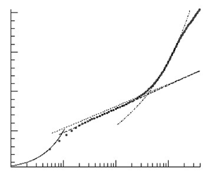
Figure 9. Mean-velocity profile and least-squares fit in the log-law region at  $x=9.944\ \mathrm {m}$ (a) for $U_\infty =23\ \mathrm {m}\ \mathrm {s}^{-1}$ using $u_\tau$ from OFI and (b) for $U_\infty =36\ \mathrm {m}\ \mathrm {s}^{-1}$ using $u_\tau$ from a least-squares fit to the profile by Nickels (Reference Nickels2004) for $y^{+}<20$.
For  $U_\infty =36\ \mathrm {m}\ \mathrm {s}^{-1}$, $y^{+}_{log,min}\in [82;90]$ and $y^{+}_{log,max}\in [142;150]$ were used. The value of $\kappa =0.379\pm 0.020$ at $\Delta p_s^{+}=0.0114$ was obtained for $u_\tau$ determined by the least-squares fit to the profile by Nickels. The detailed results are given in table 5. The mean-velocity profile and the log-law fit are shown in figure 9(b). A detailed discussion of the uncertainties and their quantification is given in appendix F.2 and in table 13.
An important finding is that the outer limit of the log law is at a much smaller  $y^{+}$-value than for ZPG flows, i.e. at $0.019\delta _{99}^{+}$ for $U_\infty =23\ \mathrm {m}\ \mathrm {s}^{-1}$ and at $0.015\delta _{99}^{+}$ for $U_\infty =36\,\mathrm {m}\ \mathrm {s}^{-1}$. It is even smaller than the widely believed start of the log-law region in ZPG flows, cf. Wei et al. (Reference Wei, Fife, Klewicki and McMurtry2005) and Marusic et al. (Reference Marusic, Monty, Hultmark and Smits2013). This indicates that, at a given significant value of, say, $\Delta p_s^{+}>0.01$, the extent of the log law cannot be simply increased by increasing $\textit {Re}$. This is different to the traditional view for ZPG, where the log law is associated with an overlap region, whose extent in terms of $y^{+}$ can be increased by increasing $\textit {Re}$. At APG, a half-power law is found instead in a large part of the overlap region, and its extent can be increased by increasing $\textit {Re}$, see § 4.6.
4.4. Clauser chart method
For the study of the CCM at APG, the same statistical evaluation as in § 4.3 was used. For  $U_\infty =23\ \mathrm {m}\ \mathrm {s}^{-1}$, $u_\tau =0.5037\ \mathrm {m}\ \mathrm {s}^{-1}$ is obtained. The sensitivity of $u_\tau$ to the values for $\kappa$ and $B$ calibrated for ZPG is smaller than $0.3\,\%$, given that the upper and lower bounds for the log-law region are fixed. The uncertainties are summarised in table 14 in appendix F.3. For $U_\infty =36\ \mathrm {m}\ \mathrm {s}^{-1}$, $u_\tau =0.7710\ \mathrm {m}\ \mathrm {s}^{-1}$ is obtained, and the uncertainties are given in table 15. The values for $u_\tau$ by the Clauser chart are systematically lower than from OFI and from the viscous sublayer fit, in agreement with Monty et al. (Reference Monty, Harun and Marusic2011).
4.5. Von Kármán constant and log-law intercept
The values for  $\kappa$ and $B$ are correlated with the pressure gradient parameter. In figure 10(a) $\kappa$ is plotted vs $\Delta p_s^{+}$, as proposed by Nickels (Reference Nickels2004), see correlation (A7). The error bars for both quantities $\Delta p_s^{+}$ and $\kappa$ are also included. The details of the uncertainty analysis are described in appendix F.2. The uncertainty of $\Delta p_s^{+}$ uses an assumed uncertainty of $3.5\,\%$ for $(1/\rho )(\mathrm {d}P_\mathrm {w}/\mathrm {d}s)$ and an uncertainty of $1 \,\%$ for $\nu$. The symbols indicate the method used to determine $u_\tau$. The values for $\kappa$ are found to be smaller for $U_\infty =23\ \mathrm {m}\ \mathrm {s}^{-1}$ than for $U_\infty =36\ \mathrm {m}\ \mathrm {s}^{-1}$. This is consistent with the proposal by Nickels in the sense that $\kappa$ is decreasing with increasing values of $\Delta p_s^{+}$. For the reference value at ZPG, $\kappa =0.40\pm 0.02$ is assumed. Thus a reduction of $\kappa$ at APG is found compared to $\kappa =0.40$, but this reduction is within the estimated uncertainty bounds.

Figure 10. (a) Value of  $\kappa$ vs $\Delta p_s^{+}$. The symbols show the method for $u_\tau$. Two-dimensional ${\mu }$PTV data for $U_\infty =23\ \mathrm {m}\ \mathrm {s}^{-1}$: $\blacksquare$, OFI; $\blacklozenge$, fit to $u^{+}=y^{+}$; $\blacktriangleright$, fit to profile by Nickels (Reference Nickels2004); $\blacktriangle$, Clauser chart. Three-dimensional LPT data for $U_\infty =36\ \mathrm {m}\ \mathrm {s}^{-1}$: $\vartriangle$, Clauser chart; $\triangleright$, fit to profile by Nickels (Reference Nickels2004); $\triangledown$, Clauser chart with empirical correction. The 2D2C PIV data using OFI for $u_\tau$: $\lozenge$, $x=8.12\ \mathrm {m}$ at almost ZPG; solid line, correlation by Nickels (Reference Nickels2004) for $\kappa _0=0.39$; dashed line, correlation by Nickels (Reference Nickels2004) using $\kappa _0=0.40$. (b) Plot of $\kappa B$ and vs $B$. Same symbols as in (a); solid line, correlation by Monkewitz et al. (Reference Monkewitz, Chauhan and Nagib2008).
Moreover, a significant role of the method to determine  $u_\tau$ is observed. The standard CCM yields lower values for $u_\tau$, and hence larger values for $\Delta p_s^{+}$, and smaller values for $\kappa$ are obtained. This gives a warning that a possible change of $\kappa$ may appear enlarged, if a standard CCM is used to determine $u_\tau$.
Regarding the intercept  $B$, the values for $\kappa B$ are plotted against $B$ in figure 10(b) and follow closely the correlation proposed by Monkewitz et al. (Reference Monkewitz, Chauhan and Nagib2008).
4.6. On the half-power-law region
Then the hypothesis of a half-power-law region (or sqrt-law region) above the log law is studied, see question (Q3) in the introduction. The mean velocity slope diagnostic function (A8a,b) is used to identify the region where the mean-velocity profile can be described by the sqrt law (1.3) following the method for ZPG turbulent boundary layers by Österlund et al. (Reference Österlund, Johansson, Nagib and Hites2000) and Monkewitz, Chauhan & Nagib (Reference Monkewitz, Chauhan and Nagib2007). For  $U_\infty =23\ \mathrm {m}\ \mathrm {s}^{-1}$, the mean-velocity profile and the fit to the sqrt law are shown in figure 11(a) for the 2D2C PIV data evaluated by the single-pixel ensemble correlation method and $u_\tau$ from OFI. The least-squares fit of (1.3) to the data is computed in the region where the slope diagnostic function (A8a,b) gives a small plateau, see figure 11(b). The single-pixel data show an approximative plateau in the region $500<y^{+}<860$, whereas the window correlation data are smoother and show a slightly smaller plateau for $520<y^{+}<840$. The outer edge of the approximative plateau $y^{+}\approx 840$ corresponds to $0.122\delta _{99}^{+}$.

Figure 11. The 2D2C PIV results at APG for  $U_\infty =23\ \mathrm {m}\ \mathrm {s}^{-1}$ at $x=9.944\ \mathrm {m}$. (a) Log-law and sqrt-law regions. (b) Mean-velocity slope diagnostic function of the sqrt law.
For  $U_\infty =36\ \mathrm {m}\ \mathrm {s}^{-1}$ the mean-velocity profile and the fit to the sqrt law are shown in figure 12(a) for the three-dimensional LPT data. A region of an approximative plateau for the slope diagnostic function (A8a,b) can be observed for $y^{+}>750$ which extends up to approximately $y^{+}\approx 1260$, see figure 12(b). The outer edge $y^{+}\approx 1260$ corresponds to $0.129\delta _{99}^{+}$. The outer limit of the plateau in terms of $y^{+}$ is increasing with increasing $U_\infty$, i.e. with increasing $\textit {Re}$. This is similar to the behaviour of the outer edge of the log law in turbulent boundary layers at ZPG. We note that the mean-velocity profile cannot be fitted by the sqrt law (1.3) in the entire inner region, say, $y^{+}\in [150,0.13\delta _{99}^{+}]$.

Figure 12. Three-dimensional LPT STB results for  $U_\infty =36\ \mathrm {m}\ \mathrm {s}^{-1}$ at $x=9.944\ \mathrm {m}$. (a) Log-law and sqrt-law regions. (b) Mean-velocity slope diagnostic function of the sqrt law.
The outer limit of the plateau is smaller than  $y/\delta =0.15$ found for ZPG by Marusic et al. (Reference Marusic, Monty, Hultmark and Smits2013), where the boundary layer thickness $\delta$ was determined from a fit of the composite law of the wall/law of the wake. The value $0.15\delta$ given in Marusic et al. (Reference Marusic, Monty, Hultmark and Smits2013) corresponds to $0.195 \delta _{99}$ if assuming that $\delta =1.3\delta _{99}$. An estimate of historical effects using $2\delta _{t.o.}$ based on $u^{*}=k^{1/2}$ in figure 5(c) gives $2\delta _{t.o.}=0.8\delta _{99}$ at $y=0.13\delta _{99}$, $2\delta _{t.o.}=1.0\delta _{99}$ at $y=0.15\delta _{99}$ and $2\delta _{t.o.}=1.7\delta _{99}$ at $y=0.2\delta _{99}$. Therefore, the outer limit of the plateau of $\xi _{sqrt}$ and the deviation of the mean-velocity profile from the sqrt-law fit above $y^{+} \geqslant 0.15\delta _{99}$ could be affected by historical effects, leading to a smaller outer limit of the sqrt law than for the log law at ZPG, see § 5. The inner limit of the plateau is larger than the value $y^{+}=350$ inferred from the relation $y^{+}=3\textit {Re}_\tau ^{1/2}$ for ZPG by Marusic et al. (Reference Marusic, Monty, Hultmark and Smits2013), assuming again $\textit {Re}_\tau =\delta ^{+}\approx 1.3\delta _{99}^{+}$.
Regarding the significant variation in scatter for figures 11(b) and 12(b), we note that the gradients for the 2D2C PIV data in figure 11(b) are computed using a central difference scheme for the unfiltered data. For the three-dimensional LPT data in figure 12(b), a two-step method was used. In the first step a smoothing of the data was applied, using a Gaussian filter with a kernel of 7 points, i.e. using the data points  $i-3,\ldots ,i+3$ for data point $i$. To compute the gradient at $y=y_i$, a linear function was fitted to the data points $y_{i-3},\ldots ,y_i,\ldots ,y_{i+3}$ using a least-square fit. Note that $y_{i+3}-y_i=8.7\delta _\nu$ can be seen as the half filter width for smoothing, see also appendix D.
The mean-velocity profile above the square-root-law region looks different from the wake of a turbulent boundary layer at APG on a flat plate, see figures 11(a) and 12(a). This originates from the upstream region of convex surface curvature and streamwise changing pressure gradient and will be described in § 5.
The value for  $K_{o}$ was determined by a least-square fit to (1.3), yielding $K_{o}=0.310$ and $B_o = -6.39$ for the single-pixel data at $U_\infty =23\ \mathrm {m}\ \mathrm {s}^{-1}$ and $u_\tau$ from OFI, and $K_{o}=0.320$ and $B_o = -4.66$ for the three-dimensional LPT STB data at $U_\infty =36\ \mathrm {m}\ \mathrm {s}^{-1}$, where $u_\tau$ from the least-squares fit to the profile by Nickels was used. For the comparison of $K_{o}$ with values reported in the literature, note that some authors use the form for the half-power law for zero-skin-friction flow by Stratford (Reference Stratford1959)
 \begin{equation} U(y)=\frac{2}{K}\left(\frac{1}{\rho}\frac{\mathrm{d}P}{\mathrm{d}s}\right)^{1/2}y^{1/2} \end{equation}
instead of (1.3). Stratford used a value of  $K=0.66\kappa =0.27$ for his zero-skin-friction flow. For the same data, Townsend (Reference Townsend1960) found $K=0.5\pm 0.05$, whereas Mellor (Reference Mellor1966) found that, at most, $K=0.44$ by excluding certain near-wall points. From the DNS by Spalart & Leonard (Reference Spalart and Leonard1986), $K=0.6$ was found. For flows with a non-zero skin friction, some representative values are $0.48\pm 0.03$ by Townsend (Reference Townsend1961), $0.48$ by Perry (Reference Perry1966), for large values of $(\delta /\tau _{w})(\mathrm {d}P/\mathrm {d}s)$, $0.45$ by Kader & Yaglom (Reference Kader and Yaglom1978) and $0.57$ by Afzal (Reference Afzal2008). The values depend on the form of the half-power law, i.e. (1.3) or (4.1), and on the region considered for the least-squares fit. For example, if the half-power-law fit is applied above the log-law region, as proposed by Perry (Reference Perry1966), then smaller values are obtained than if the fit is applied to all data in the inner layer above the buffer layer. The latter method was used e.g. by Afzal (Reference Afzal2008). The values obtained for $K_{o}$ for the present flow are smaller than other values reported in the literature, despite these details.
As a final remark, Perry (Reference Perry1966) proposed an extension of his three-layer model, suggesting that the first and second streamwise derivatives of the pressure gradient might need to be included to account for effects of a streamwise decreasing APG. He proposed a region IV above the half-power-law region, where the mean-velocity gradients are proportional to  $y^{0}$ (compared to $y^{-1}$ in the log-law region and $y^{-1/2}$ in the half-power-law region) and are governed by ${\rm d}^{2} P/{\rm d}s^{2}$. Such a region was also proposed by Durbin & Belcher (Reference Durbin and Belcher1992) for reasons of matching with the outer part of the boundary layer and called the middle region. For the present data, a region where $U\sim y$ can be observed from $y^{+}=3500$ to $y^{+}=5000$, corresponding to $0.35<y/\delta _{99}<0.51$.
4.7. Summary
The log law in the mean-velocity profile was found to be a robust feature at APG, but its region is thinner than in zero pressure gradient flows (Q1). The von Kármán constant  $\kappa$ was found to be reduced, but within the uncertainty of the measurement (Q2). A square-root law was observed to emerge above the log law in a large part of the region the log law occupies at ZPG (Q3).
5. Streamwise evolution of the mean velocity
As the focus is on the mean flow scaling and given that the inner and outer regions are connected by an overlap region, history effects for the inner and outer layer need to be discussed. Perry et al. (Reference Perry, Bell and Joubert1966) divided the boundary layer into a ‘wall region’ and a ‘historical region’. In the wall region, only the local flow quantities  $\mathrm {d}P/{\mathrm {d}s}$, $\tau _{w}/\rho$, and $y$ govern the mean-velocity profile, and higher derivatives of $\mathrm {d}P/{\mathrm {d}s}$ and $\tau _{w}/\rho$ may be involved above a certain wall distance. In the historical region, the mean-velocity profile is influenced by ‘upstream events’. To better understand the mean-velocity profile at the APG focus position $x=9.944\ \mathrm {m}$, the local effects and the historical effects of streamwise changing pressure gradient, convex curvature and relaxation from curvature are discussed as the flow evolves downstream. The history effects in the outer region are quantified using the shape factor $H_{12}$ due to the issues in the definition of the wake parameter, see Chauhan et al. (Reference Chauhan, Monkewitz and Nagib2009) for ZPG flows. Table 6 gives the streamwise positions studied. The distance $x^{*}_{curv}=(x-x_b)/\delta _{99,{ref}}$ from the beginning of curvature at $x_b=8.990\ \mathrm {m}$ is defined as a multiple of $\delta _{99,{ref}}$, and $x^{*}_{relax} = (x-x_e)/\delta _{99,{apg}}$ defines the distance of flow relaxation downstream of the end of curvature, measured from the end of curvature at $x_e=9.750\ \mathrm {m}$, as a multiple of $\delta _{99,{apg}}=0.17\ \mathrm {m}$ at $x=9.72\ \mathrm {m}$.
Table 6. Positions for the mean-flow profiles from the 2D2C PIV overview measurement. The values are for the case  $U_\infty =23\ \mathrm {m}\ \mathrm {s}^{-1}$ using the values for $u_\tau$ obtained by OFI.

The change from ZPG to FPG causes a reduction of  $H_{12}$ and of the wake factor $\varPi$, which is known for FPG, see, e.g. Jones, Marusic & Perry (Reference Jones, Marusic and Perry2001). Moreover, a downward shift of the entire $u^{+}$-profile by $\Delta u^{+}=-0.4$ is observed, see figure 13(a). This shift is not observed if $u_\tau$ from the CCM is used, giving 2 % to 3 % larger values for $u_\tau$, close to the uncertainty of 2 % of the OFI method. As the FPG becomes strongest near $x=9.12\ \mathrm {m}$ and curvature effects increase, the extent of the log-law region is observed to be reduced to $y^{+}<450$ (or $y/\delta _{99}<0.047$), and above, the velocity profile, plotted against $\log (y^{+})$, turns downwards below the log law. Regarding the reduction of $\varPi$, the acceleration parameter $K=-\nu /U_e^{2} \,\mathrm {d}U_e/\mathrm {d}s$ quantifying the strength of the FPG is $K= 1.0\times 10^{-7}$. Hence, $K$ and $\Delta p_s^{+}$ are smaller than for the smallest FPG case $K=2.7\times 10^{-7}$ and $\Delta p_s^{+}=-3.3\times 10^{-3}$ in Jones et al. (Reference Jones, Marusic and Perry2001). Then the pressure gradient rapidly changes from increasing to decreasing FPG. History effects in the outer layer are found at $x=9.32\ \mathrm {m}$, where $\beta _{RC}$ is (almost) zero. Here $H_{12}$ remains at the low value of $H_{12}=1.20$ at $x=9.12\ \mathrm {m}$ and is significantly smaller than $H_{12}=1.25$ in the upstream ZPG region.

Figure 13. Mean-velocity profiles for  $U_\infty =23\ \mathrm {m}\ \mathrm {s}^{-1}$ at almost ZPG and in the region of curvature with change from favourable to APG.
The APG region on the curved wall ( $x\geqslant 9.32\ \mathrm {m}$) is shown in figure 13(b). In the inner layer, the value of $u^{+}$ at $y^{+}=100$, denoted by $u^{+}(100)$, remains almost unaltered. For $y^{+}>200$ (or $y/\delta _{99}>0.024$), the profiles begin to turn upwards above the log law. This is mainly attributed to the APG, which reaches $\Delta p_s^{+}=0.005$ at $x=9.52\ \mathrm {m}$. Note that a reduction of the log-law region and an upward turn above the log law was also observed in convex curvature flows at ZPG by Gillis et al. (Reference Gillis, Johnston, Kays and Moffat1980), and by Kim & Rhode (Reference Kim and Rhode2000). However, the upward turn, quantified by $\Delta u^{+}(y^{+})$ above the log law, shown therein is smaller than for the present flow. Regarding the outer layer, $H_{12}$ is rising downstream of $x>9.32\ \mathrm {m}$ due to the APG, albeit convex curvature was also found to cause a small increase of $H_{12}$, see Patel & Sotiropoulos (Reference Patel and Sotiropoulos1997). Another historical effect is found at $x=9.52\ \mathrm {m}$, where $H_{12}$ reaches again the value from the ZPG region, albeit at $\beta _{RC}=4.5$ and with a different form of the mean-velocity profile.
Downstream of the end of curvature at  $x=9.750\ \mathrm {m}$, the flow is subjected to an APG and relaxation from curvature. The mean-velocity profiles are shown in figure 14(a). Regarding the inner layer, the value for $u^{+}(100)$ appears still to be almost unchanged. The upward turn above the log law is increasing in downstream direction, consistent with the increase of the slope of the square-root law with increasing $\Delta p_s^{+}$. For $x\geqslant 9.944\ \mathrm {m}$, $u^{+}(100)$ is found to be decreasing, and in the log-law region the profiles appear to be shifted below the log law at ZPG, see figure 14(b). The log-law region appears to recover as the flow relaxes from curvature. The recovery for the ZPG case is described in Gillis et al. (Reference Gillis, Johnston, Kays and Moffat1980) and Alving et al. (Reference Alving, Smits and Watmuff1990). In the square-root-law region, the slope of $u^{+}$ is continuously increasing, consistent with the increasing $\Delta p_s^{+}$ values. Regarding the outer layer, $\varPi$ and $H_{12}$ are further increasing due to the APG, but remain substantially smaller than for the corresponding equilibrium flow.

Figure 14. Mean-velocity profiles for  $U_\infty =23\ \mathrm {m}\ \mathrm {s}^{-1}$ in the APG region.
The cumulative history effect of the present flow is studied in terms of the defect shape factor  $G$, where $H_{12}=(1-\gamma G)^{-1}$ with $\gamma =u_\tau /U_{e}$ to account for $\textit {Re}$-effects, and compared with the theory for equilibrium turbulent boundary layer flows by Mellor & Gibson (Reference Mellor and Gibson1966). Together with the streamwise distribution of $\beta _\mathrm {RC}$ given in figure 4(b), figure 15(a) shows the delayed response of $G$ for the present flow compared to the corresponding equilibrium flow at the same value of $\beta _{RC}$.

Figure 15. (a) Defect shape factor  $G$ for $U_\infty =23\ \mathrm {m}\ \mathrm {s}^{-1}$ and theory for equilibrium flows by Mellor & Gibson (Reference Mellor and Gibson1966) with the data by Bradshaw in Coles & Hirst (Reference Coles and Hirst1969). (b) Mean velocity for $U_\infty =36\ \mathrm {m}\ \mathrm {s}^{-1}$ at $x=9.944\ \mathrm {m}$ and data by Schubauer & Klebanoff in Coles & Hirst (Reference Coles and Hirst1969) at similar local flow conditions $\Delta p_s^{+}$ and $\Delta u_{\tau ,s}^{+}$, see (E2a–c).
Between the outer edge of the square-root law and the wake, an  $S$-shaped bending in the $u^{+}$-profile is observed, if plotted against $\log (y^{+})$, appearing at $x = 9.42\ \mathrm {m}$ and persisting downstream. From the flow history, the $S$-shaped bending appears as a combined effect of the upward turn above the log law due to the APG, starting to grow for $x\geqslant 9.42\ \mathrm {m}$, and the downward turn below the log law originating in the upstream FPG region. This could be a non-equilibrium effect due to the rapid change in $u_\tau$ and in ${\rm d}P/{\rm d}s$ over a short streamwise distance, see Spalart (Reference Spalart2010).
Finally, the role of local and historical effects on the mean velocity in the inner layer are discussed for the high- $\textit {Re}$ case, given that the inner and outer layer are connected by an overlap region. For the local effects $\Delta p_s^{+}$ and the wall shear stress gradient parameter $\Delta u_{\tau ,s}^{+}$ are considered, motivated by the model for the total shear stress (E2a–c), where $\Delta u_{\tau ,s}^{+}$ describes the local flow acceleration. Figure 15(b) compares the present data with two profiles by Schubauer & Klebanoff (denoted by 2134 and 2135 in Coles & Hirst Reference Coles and Hirst1969) at almost the same values of $\Delta p_s^{+}$, $\Delta u_{\tau ,s}^{+}$ and $\textit {Re}_\theta$, see table 7. Error bars with a relative magnitude of 5 % for $u^{+}$ and 6 % for $y^{+}$ are included, based on the relative uncertainty in $u_\tau$ of $5\,\%$ and in $\nu$ of $1\,\%$. In the inner layer, the reduction of the log-law region and the emerging of the sqrt law above the log law are similar for the two flows. One should be cautious, however, due to the uncertainty of the $u_\tau$-values reported in Coles & Hirst (Reference Coles and Hirst1969) which rely on the CCM with $\kappa =0.41$ and $B=5.0$, see § 4.4, and deviations of the $u^{+}$-profiles within the error bounds are possible. The comparable inner layer behaviour indicates the influence of the local effects and the rapid response of the inner layer. The differences in the outer layer are due to the different flow history, leading to larger values $H_{12}=1.86$ and $H_{12}=1.98$ for the flow by Schubauer & Klebanoff. For comparison, $H_{12}=2.0$ was found for the equilibrium flow by Skare & Krogstad (Reference Skare and Krogstad1994) at almost the same $\Delta p_s^{+}$, $\textit {Re}_\theta$ and $\beta _{RC}$, but at a much smaller $\Delta u_{\tau ,s}^{+}$. These findings are in agreement with the result by Bobke et al. (Reference Bobke, Vinuesa, Örlü and Schlatter2017), that $\beta _{RC}$ alone is not sufficient to determine the mean-velocity profile at APG. A more detailed view reveals that the extent of the sqrt law is a little smaller for the present flow than for the flow by Schubauer & Klebanoff. This is an indication that the outer part of the inner layer is probably affected by historical effects of the outer layer.
Table 7. Summary of local flow parameters for APG flows shown in figure 15(b).

To summarise, the observed rapid recovery of the log-law region downstream of the end of curvature is in agreement with the results for the eddy turnover length  $\delta _{{t.o.}}$ in figure 5(c), indicating that the inner layer relaxes rapidly, albeit not instantaneously. The mean velocity in the outer layer was found to be influenced by history effects due to streamwise changing pressure gradient and convex curvature in conjunction with the slow response of the outer layer indicated by the large values for $\delta _{{t.o.}}$. The history effects were found to affect the outer part of the inner layer, causing the observed reduced extent of the sqrt-law region compared to the region occupied by the log law at ZPG.
6. Conclusions
The goal of the analysis was to determine the resilience of the log law for the mean velocity, the possible change of the von Kármán constant  $\kappa$ and the appearance of a square-root law above the log law at significant APGs. We observed that, while the log law in the mean-velocity profile is a robust feature at APG, this region is thinner than its ZPG counterpart, and its slope is altered. A square-root law emerges above the log law in a large part of the region the log law occupies at ZPG. The square-root law was detected by a plateau of the mean-velocity slope diagnostic function. As the plateau was found to have only a moderate extent even for the large Reynolds number $\textit {Re}_\theta =57\,000$, we infer that the square-root-law region appears only at sufficiently large Reynolds numbers. This structure of the mean velocity profile confirms the proposal by Perry et al. (Reference Perry, Bell and Joubert1966).
It was found that, when the pressure gradient parameter  $\Delta p_s^{+}$ increases from zero to $0.018$, the value of $\kappa$ decreases from $0.395\pm 0.013$ to $0.370\pm 0.017$. For comparison, the model by Nickels (Reference Nickels2004) predicts a reduction from $\kappa =0.390$ for $\Delta p_s^{+}=0$ to $\kappa =0.365$ for $\Delta p_s^{+}=0.018$. Using the value for $u_\tau$ from the Clauser chart was shown to give erroneously smaller values for $\kappa$ than if a direct method for $u_\tau$ was used. The reduction of $\kappa$ could not be demonstrated to be significant due to the measurement uncertainty, and because of possible history effects of the upstream located region of streamwise changing pressure gradient and convex wall curvature. The major contribution to the overall uncertainty of $\kappa$ stems from the wall shear stress. Complementary to OFI, two indirect methods for the wall shear stress were found to be promising, viz., using a least-squares fit to the mean-velocity profile by Nickels (Reference Nickels2004) in the region $y^{+}<20$, and the relation for the total shear stress derived from the integral form of the mean momentum balance, see Volino & Schultz (Reference Volino and Schultz2018).
Finally the findings are put in context with other turbulent boundary layer flows at APG. In the inner layer, the reduction of the log-law region and the emerging of the sqrt law above the log law were found to be similar to the flow by Schubauer & Klebanoff in Coles & Hirst (Reference Coles and Hirst1969). Both data are at a similar  $\textit {Re}_\theta$ and $\beta _{RC}$, and at almost the same values for $\Delta p_s^{+}$ and wall shear stress gradient parameter $\Delta u_{\tau ,s}^{+}$. This indicates the rapid response of the inner layer and the role of local effects on the inner layer. Significant historical effects were observed for the outer layer, and these were found to affect the outer part of the inner layer and the extent of the sqrt-law region. As most turbulent boundary layer flows of practical relevance are streamwise evolving flows, future research on non-equilibrium and history effects seems to be highly appreciated.
Acknowledgements
The authors gratefully acknowledge the assistance of M. Bitter, F. Eich, R. Hain, S. Scharnowski, J. Agocs and R. Geisler for the wind-tunnel experiment. The authors are very grateful to the partners of the International Collaboration on Experimental Turbulence (ICET) and in particular to S.C.C. Bailey and to I. Marusic for kindly providing their data. Finally the very valuable reviewer comments are gratefully acknowledged.
Funding
The experiment was funded by DFG (Grant KA 1808/14-1 & SCHR 1165/3-1) and by the DLR Institute of Aerodynamics and Flow Technology.
Declaration of interests
The authors report no conflict of interest.
Appendix A. Theoretical relations
A.1. Boundary layer theory and scaling to viscous units
Consider a two-dimensional, incompressible turbulent boundary layer flow. A wall-fitted local coordinate system with streamwise wall-parallel direction  $s$, wall-normal direction $y$ and mean-velocity components $U$ (streamwise wall parallel) and $V$ (wall normal) is assumed together with the following boundary layer equation for $U$
$U$
 \begin{equation} \nu\frac{\partial^{2} U}{\partial y^{2}} - \frac{\partial \overline{u'v'}}{\partial y} = \frac{1}{\rho}\frac{\mathrm{d} P_{w}}{\mathrm{d} s} +U\frac{\partial U}{\partial s} +V\frac{\partial U}{\partial y} + \frac{\partial }{\partial s}\left(\overline{u'^{2}}-\overline{v'^{2}}\right). \end{equation}
Here, the relation  $P(s,y)= P_{w}(s)-\overline {v'^{2}}(s,y)$ is used, which can be obtained by integration of the boundary layer equation for $V$, see Hinze (Reference Hinze1975). Then integration of (A1) from the wall to the wall distance $y$ gives the following relation for the total shear stress $\tau$
 \begin{align} \frac{\tau}{\rho}
&\equiv \nu\frac{\partial U}{\partial y}- \overline{u'v'}
=\frac{\tau_w}{\rho} +\frac{1}{\rho}\frac{\mathrm{d}
P_\mathrm{w}}{\mathrm{d} s} y +\int_{0}^{y}U\frac{\partial
U}{\partial s}\,\mathrm{d}\tilde{y}
\notag\\ &\quad +\int_{0}^{y}V\frac{\partial U}{\partial
\tilde{y}}\,\mathrm{d}\tilde{y}+\int_{0}^{y}\frac{\partial
}{\partial
s}\left(\overline{u'^{2}}-\overline{v'^{2}}\right)\mathrm{d}\tilde{y},
\end{align}
\begin{align} \frac{\tau}{\rho}
&\equiv \nu\frac{\partial U}{\partial y}- \overline{u'v'}
=\frac{\tau_w}{\rho} +\frac{1}{\rho}\frac{\mathrm{d}
P_\mathrm{w}}{\mathrm{d} s} y +\int_{0}^{y}U\frac{\partial
U}{\partial s}\,\mathrm{d}\tilde{y}
\notag\\ &\quad +\int_{0}^{y}V\frac{\partial U}{\partial
\tilde{y}}\,\mathrm{d}\tilde{y}+\int_{0}^{y}\frac{\partial
}{\partial
s}\left(\overline{u'^{2}}-\overline{v'^{2}}\right)\mathrm{d}\tilde{y},
\end{align}
where  $\tau _w$ denotes the wall shear stress. The classical scaling to inner viscous units reads
 \begin{equation} u^{+}=\frac{U}{u_\tau},\quad y^{+}=\frac{y u_\tau}{\nu},\quad \tau^{+}=\frac{\tau}{\tau_w}, \quad u_\tau=\sqrt{\frac{\tau_w}{\rho}},\quad \Delta p^{+}=\frac{\nu}{\rho u_\tau^{3}}\frac{\mathrm{d} P_{w}}{\mathrm{d}s}. \end{equation}
A second classical scaling based on the so-called pressure–viscosity velocity  $u_p=\nu /\rho |\mathrm {d}P_{w}/\mathrm {d}s|$ by Stratford (Reference Stratford1959) and Mellor (Reference Mellor1966) is not used in this work, since $u_\tau >10 u_p$ in the region of interest of the present work.
A.2. Relations for the mean velocity at APGs
A.2.1. A model for the viscous sublayer thickness by T. Nickels
Nickels (Reference Nickels2004) proposes an analytical model for the mean velocity in boundary layers subjected to mild and moderately strong pressure gradients, which can be favourable and adverse. The viscous sublayer solution  $U_{vis}^{+}=U_{vis}^{+}(y^{+};\Delta p_s^{+},y_c^{+})$ is given by
 \begin{align} U_{{vis}}^{+}=y_c^{+}\left[1-\left[1+2\frac{y^{+}}{y_c^{+}}+\frac{1}{2}\left(3-\Delta p_s^{+}y_c^{+}\right) \left(\frac{y^{+}}{y_c^{+}}\right)^{2}-\frac{3}{2}\Delta p_s^{+}y_c^{+}\left(\frac{y^{+}}{y_c^{+}}\right)^{3}\right] \textrm{e}^{{-}3({y^{+}}/{y_c^{+}})} \right], \end{align}
which depends on the local value of  $\Delta p_s^{+}$ and a parameter $y_c^{+}$, which is associated with the thickness of the viscous sublayer. Then $y_c$ is determined by a stability argument using a critical value $\textit {Re}_c$ of a suitably defined local Reynolds number
 \begin{equation} \textit{Re}_c=\frac{u_Ty_c}{\nu},\quad u_T=\left(\frac{\tau|_{y=y_c}}{\rho}\right)^{1/2}, \quad \tau^{+}|_{y=y_c}=1+\Delta p_s^{+}y_c^{+} . \end{equation}
Here,  $y_c$ is the critical value of $y$ above which the viscous sublayer becomes unstable. The assumption that $\textit {Re}_c$ has a universal value for all wall-bounded flows implies that
 \begin{equation} \Delta p_s^{+}\left(y_c^{+}\right)^{3}+\left(y_c^{+}\right)^{2}-\textit{Re}_c^{2}=0, \end{equation}
where  $\textit {Re}_c$ is the only free parameter and is chosen from ZPG data to $\textit {Re}_c=12$. The physically relevant solution for $y_c$ is the smallest positive root of (A6).
A.2.2. A model for the von Kármán constant $\kappa$ by T. Nickels

Regarding the von Kármán constant  $\kappa$, Nickels (Reference Nickels2004) argues that two relations to characterise the vorticity scale in the inner layer should be equal. The first relation is based on the velocity scale $u_\tau$ and the second is based on $u_T$. This leads to
 \begin{equation} \frac{\partial U}{\partial y}=\frac{u_T}{\kappa_0 y}=\frac{u_\tau}{\kappa y} \quad\Leftrightarrow\quad \frac{\kappa}{\kappa_0}=\frac{u_\tau}{u_T} \quad\Leftrightarrow\quad \frac{\kappa}{\kappa_0}=\sqrt{\frac{1}{1+\Delta p_s^{+}y_c^{+}}} \end{equation}
where  $\kappa _0$ is the value of $\kappa$ for the ZPG case, for which $\kappa _0=0.39$ is chosen.
A.2.3. Mean-velocity slope diagnostic functions
The mean-velocity slope diagnostic function is a method to assess the functional behaviour of the mean-velocity gradient, see e.g. Österlund et al. (Reference Österlund, Johansson, Nagib and Hites2000) for ZPG flows. The diagnostic functions for log law and sqrt law (1.3) are
 \begin{equation} \xi_{log}^{{-}1}=y^{+}\left(\frac{\mathrm{d}u^{+}}{\mathrm{d}\kern 0.05em y^{+}}\right)_{data}\,,\quad \xi_{sqrt}^{{-}1}=\frac{y^{+}}{\sqrt{1+\Delta p_s^{+}y^{+}}}\left(\frac{\mathrm{d}u^{+}}{\mathrm{d} y^{+}}\right)_{data}. \end{equation}
A plateau region of the slope diagnostic function supports the assumed behaviour of  $u^{+}(y^{+})$. At ZPG, a plateau can be seen only for $\textit {Re}_\theta >rapprox 6000$, see Österlund et al. (Reference Österlund, Johansson, Nagib and Hites2000). The overlap of inner and outer layer becomes sufficiently thick in terms of $y^{+}$ only for asymptotically high $\textit {Re}$. At APG, we suppose that at least $\textit {Re}_\theta >10\,000$ is needed to observe an asymptotic behaviour with a sufficiently thick overlap region. This was found in a study of the database by Coles & Hirst (Reference Coles and Hirst1969) in Knopp (Reference Knopp2016).
Appendix B. Flow conditions during the wind-tunnel measurements
The flow conditions for the different measurement campaigns are summarised in table 8. The reference pressure  $p_\infty$ was measured downstream of the contour model near the exit of the test section.
Table 8. Summary of flow conditions in the wind tunnel.

Appendix C. Determination of the boundary layer thickness
As a boundary layer at APG exists below irrotational free streams with non-zero wall-normal variations, Coleman et al. (Reference Coleman, Rumsey and Spalart2018) proposed  $\tilde {\delta }_{99}$ based on the velocity $\tilde {U}$
 \begin{equation} \tilde{U}(s,y)={-}\int_0^{y} \bar{\omega}_z(s,y')\,\mathrm{d} y',\quad \bar{\omega}_z =\frac{\partial V}{\partial s}-\frac{\partial U}{\partial y} \end{equation}
In the APG region on the inclined flat plate, the difference between  $\delta _{99}$ and $\tilde {\delta }_{99}$ is $1\,\%$. An advantage of $\tilde {\delta }_{99}$ is that $\tilde {U}$ shows a clearer region of $\partial \tilde {U}/\partial y = 0$.
In the convex curvature region the pressure increases with distance to the wall, and there is a corresponding decrease in velocity in the inviscid flow. Following Patel & Sotiropoulos (Reference Patel and Sotiropoulos1997), the boundary layer thickness needs to be defined using the potential flow velocity distribution  $U_{p}=U_{pw}(1-Ky)$, where the curvature $K=1/R_{c}$ is positive for a convex wall, and $U_{pw}$ is the hypothetical potential flow velocity at the wall, which is found from $c_p$ using the Bernoulli equation. Figure 3 shows that $U(y)$ approaches $U_{p}(y)$ at $x=9.42\ \mathrm {m}$ in the region of approximately constant surface curvature. The wall distance, where $U$ reaches $0.99U_{p}$, is $\delta =0.144\ \mathrm {m}$ compared to $\delta _{99}=0.131\ \mathrm {m}$.
Moreover, the two criteria proposed in Vinuesa et al. (Reference Vinuesa, Bobke, Örlü and Schlatter2016) were studied, i.e. the wall distance where (i)  $u'/U=0.02$ and (ii) where $u'/(U\sqrt {H_{12}})=0.02$. The former gives better agreement with $\delta _{99}$ and $\tilde {\delta }_{99}$. It shows slightly smaller values than $\delta _{99}$. The deviation is below $5\,\%$ in the ZPG region and $3.7\,\%$ on the flat wall in the APG region. Finally, the results for the TNTI by Reuther & Kähler (Reference Reuther and Kähler2018) are used, which were evaluated using an intermittency factor of $\gamma =0.3$, see Reuther (Reference Reuther2019). The deviation of $\delta _{99}$ from these values is smaller than $2.5\,\%$ in the ZPG region and $4\,\%$ in the curvature region. In the APG region, the values are up to $7.5\,\%$ larger than $\delta _{99}$.
Appendix D. Mean-velocity slope diagnostic function for the log-law
The mean-velocity slope diagnostic function for the three-dimensional LPT data for the case  $U_\infty =36\ \mathrm {m}\ \mathrm {s}^{-1}$ is shown in figure 16(a). The smoothing method described in § 4.6 was applied to the data. An approximative plateau is found in the region $84<y^{+}<152$.

Figure 16. (a) Mean-velocity slope diagnostic function for the log law for  $U_\infty =36\ \mathrm {m}\ \mathrm {s}^{-1}$. (b) Determination of $u_\tau$ by a least-square fit of the measured total shear stress (denoted by 3D LPT STB, ave) and the remaining terms of the integral momentum balance (A2), see (3) in Volino & Schultz (Reference Volino and Schultz2018). For the nomenclature see (E1a–c).
Appendix E. Method to determine the friction velocity from the mean momentum balance
In figure 16(b)  $u_\tau$ is determined by a least square fit of the total shear stress and the remaining terms of the integral mean momentum balance on the right-hand side of (A2), after scaling both sides to viscous units. Therein a $2\,\%$ error bar for the right-hand side of (A2) is shown. For abbreviation in figure 16(b), we use the notation
 \begin{align} I_{cu}(y)=\int_{0}^{y}U\frac{\partial U}{\partial s}\,\mathrm{d}\tilde{y}, \quad I_{cv}(y)=\int_{0}^{y}V\frac{\partial U}{\partial \tilde{y}}\,\mathrm{d}\tilde{y}, \quad I_{r}(y)=\int_{0}^{y} \frac{\partial }{\partial s}\left(\overline{u'^{2}}- \overline{v'^{2}}\right)\mathrm{d}\tilde{y}, \end{align}
to denote the integrated convective term and the Reynolds normal stress term. This approach corresponds to the use of (3) in Volino & Schultz (Reference Volino and Schultz2018). The estimate of an uncertainty of  $5\,\%$ for $u_\tau$ is based on the uncertainty of $3.5\,\%$ for $\rho ^{-1}\,\mathrm {d}P_{w}/\mathrm {d}s$ and of $1.5\,\%$ for the remaining terms of (E1a–c) for the three-dimensional LPT data.
E.1. A model for the total shear stress
An analytical model for the total shear stress by Coles (Reference Coles1956) and Perry (Reference Perry1966) is based on the ansatz for the mean-velocity profile in the inner region  $U(s,y)=u_\tau (s) \,f(y^{+}(s,y))$ and $y^{+}(s,y)=u_\tau (s)y/\nu$ to model (E1a–c). By neglecting $I_{r}^{+}(y^{+})$ this gives
 \begin{equation} \tau^{+}(y^{+}) =1 + \Delta p_s^{+} y^{+}+\Delta u_{\tau,s}^{+} I_{u}^{+},\quad \Delta u_{\tau,s}^{+}= \frac{\nu}{u_\tau^{2}}\frac{\mathrm{d} u_\tau}{\mathrm{d} s} \quad I_{u}^{+}=\int_0^{y^{+}} f^{2}\,\mathrm{d}\tilde{y}^{+}. \end{equation}
The local effects on the total shear stress in the inner layer involve  $\Delta p_s^{+}$ and the wall shear stress gradient parameter $\Delta u_{\tau ,s}^{+}$. Note that an extension of the ansatz (E2a–c) using $f=f(y^{+}(s,y), \Delta p_s^{+}(s))$ accounts for higher-order effects on $\tau ^{+}$, involving an additional parameter based on ${\rm d}^2P/{\rm d}s^{2}$, see Knopp et al. (Reference Knopp, Buchmann, Schanz, Eisfeld, Cierpka, Hain, Schröder and Kähler2015).
Appendix F. Uncertainty analysis
In this section the uncertainty analysis for the different methods to determine the friction velocity  $u_\tau$, and for the evaluation of $\kappa$ is presented.
F.1. Determination of the friction velocity
For the OFI results at  $U_\infty =23\ \mathrm {m}\ \mathrm {s}^{-1}$, the uncertainty in $u_\tau$ is estimated to be $2.0\,\%$. This estimate is based on the work by Thibault & Poitras (Reference Thibault and Poitras2017). For the current application case (oil viscosity is calibrated up to a standard uncertainty of $1\,\%$, re-projection of the interference images onto the model surface with an accuracy on the local scale of better than $1\,\%$, improving accuracy by statistical and local averaging of multiple independent measurements, etc.) the standard uncertainty of OFI for determining $u_\tau$ is expected to be better than ${\pm }2\,\%$ (with a $95\,\%$ confidence level). For comparison Harun et al. (Reference Harun, Monty, Mathis and Marusic2013) report an uncertainty of $1\,\%$.
For the method to determine  $u_\tau$ by a least-squares fit of the data to the relation $u^{+}=y^{+}$ in the region $y^{+}\in [2\pm 0.1; 4.6\pm 0.6]$, the sources of uncertainties are listed in table 9. For the overall uncertainty for $u_\tau$ the estimate is $4.4\,\%$.
Table 9. Uncertainty quantification for  $u_\tau$ for the least-squares fit to the viscous sublayer profile $u^{+}=y^{+}$ in the region $y^{+}\in [2; 4.6]$ for the ${\mu }$PTV data at $U_\infty =23\ \mathrm {m}\ \mathrm {s}^{-1}$.

For the method to determine  $u_\tau$ using a least-squares fit of the data to the profile by Nickels (Reference Nickels2004) in the region $y^{+}\in [2; 20]$, the sources of uncertainties are listed in table 10. The uncertainty due to the assumed profile by Nickels (Reference Nickels2004) was estimated by a statistical evaluation and comparison with the data by Nagano et al. (Reference Nagano, Tagawa and Tsuji1991), Manhart & Friedrich (Reference Manhart and Friedrich2002) and Coleman et al. (Reference Coleman, Rumsey and Spalart2018) in the interval given above, and is denoted by additional unknown systematic uncertainty. The overall uncertainty for $u_\tau$ is $3.8\,\%$.
Table 10. Uncertainty quantification for  $u_\tau$ for the least-squares fit to the profile by Nickels (Reference Nickels2004) in the region $y^{+}\in [2; 20]$ for the ${\mu }$PTV data at $U_\infty =23\ \mathrm {m}\ \mathrm {s}^{-1}$.

The sources of uncertainties for the method to determine  $u_\tau$ using a fit to the profile by Nickels (Reference Nickels2004) in the region $y^{+}\in [5; 20]$ for the three-dimensional LPT data at $U_\infty =36\ \mathrm {m}\ \mathrm {s}^{-1}$ are listed in table 11. The overall uncertainty for $u_\tau$ is estimated to be $4.0\,\%$.
Table 11. Uncertainty quantification for  $u_\tau$ for the fit to the profile by Nickels (Reference Nickels2004) in the region $y^{+}\in [5; 20]$ for the three-dimensional LPT data for $U_\infty =36\ \mathrm {m}\ \mathrm {s}^{-1}$.

F.2. Determination of the von Kármán constant $\kappa$

The sources for uncertainty for  $\kappa$ are summarised in table 12 for $U_\infty =23\ \mathrm {m}\ \mathrm {s}^{-1}$ and in table 13 for $U_\infty =36\ \mathrm {m}\ \mathrm {s}^{-1}$. The uncertainty due to the choice of the log-law region is computed by a statistical variation of $y^{+}_{log,min}$ and $y^{+}_{log,max}$, motivated by the Monte Carlo-based error analysis in Bailey et al. (Reference Bailey, Vallikivi, Hultmark and Smits2014). For $U_\infty =23\ \mathrm {m}\ \mathrm {s}^{-1}$ the lower bound was $y^{+}_{log,min}\in [82;92]$ and the upper bound was $y^{+}_{log,max}\in [126;138]$. For $U_\infty =36\ \mathrm {m}\ \mathrm {s}^{-1}$, $y^{+}_{log,min}\in [82;90]$ and $y^{+}_{log,max}\in [142;150]$ was used. The overall uncertainties for $\kappa$ are given in the last column in table 4 for $U_\infty =23\ \mathrm {m}\ \mathrm {s}^{-1}$ and in table 5 for $U_\infty =36\ \mathrm {m}\ \mathrm {s}^{-1}$.
Table 12. Sources of uncertainties for the determination of  $\kappa$ and uncertainty quantification for the ${\mu }$PTV data for $U_\infty =23\ \mathrm {m}\ \mathrm {s}^{-1}$.

Table 13. Sources of uncertainties for the determination of  $\kappa$ and uncertainty quantification for the three-dimensional LPT data for $U_\infty =36\ \mathrm {m}\ \mathrm {s}^{-1}$.

F.3. Clauser chart method in the APG region
For the uncertainty of the CCM, Monty et al. (Reference Monty, Harun and Marusic2011) report an uncertainty for  $u_\tau$ of $5\,\%$ for $\beta _{RC}\geqslant 2$. For the Preston tube, Patel (Reference Patel1965) gives an accuracy within $6\,\%$ for $\Delta p_s^{+}<0.015$, see also Brown & Joubert (Reference Brown and Joubert1969). For the present flow, the deviation of $u_\tau$ determined by the CCM is smaller than $5\,\%$ compared to the value for $u_\tau$ from the most reliable method. Therefore, a systematic error of $5\,\%$ for the CCM is assumed. Moreover, the additional sources for uncertainties need to be taken into account. The sensitivity with respect to the interval $[y^{+}_{log,min},y^{+}_{log,max}]$ is estimated by a statistical variation of the lower and upper bounds. This gives a relative uncertainty based on the ${\pm } 2\sigma$-interval of $0.65\,\%$ for $U_\infty =23\ \mathrm {m}\ \mathrm {s}^{-1}$ and a value below $0.1\,\%$ for $U_\infty =36\ \mathrm {m}\ \mathrm {s}^{-1}$. The results are summarised in table 14 for $U_\infty =23\ \mathrm {m}\ \mathrm {s}^{-1}$ and in table 15 for $U_\infty =36\ \mathrm {m}\ \mathrm {s}^{-1}$.
Table 14. Sources of uncertainties for the determination of  $u_\tau$ using the CCM and uncertainty quantification for the ${\mu }$PTV data at $U_\infty =23\ \mathrm {m}\ \mathrm {s}^{-1}$.

Table 15. Sources of uncertainties for the determination of  $u_\tau$ using the CCM and uncertainty quantification for the three-dimensional LPT data at $U_\infty =36\ \mathrm {m}\ \mathrm {s}^{-1}$.

Appendix G. Empirical correction method for the Clauser chart
An empirical method was used to correct the standard CCM for  $u_\tau$ for the three-dimensional LPT data for $U_\infty =36\ \mathrm {m}\ \mathrm {s}^{-1}$. It is based the observation found in this work and by Monty et al. (Reference Monty, Harun and Marusic2011), that the value for $u_\tau$ by the CCM is lower than the value determined by a direct method. For simplicity assume that the correction is a linear function of $\Delta p_s^{+}$ neglecting higher-order terms. Putting this together, we use the empirical correction
 \begin{equation} u_{\tau,{CCM+corr},36}=u_{\tau,{CCM},36}\left(1+\frac{u_{\tau,{vis},23}-u_{\tau,{CCM},23}}{u_{\tau,{CCM},23}}\,\frac{\Delta p_{s,36}^{+}}{\Delta p_{s,23}^{+}}\right) ,\end{equation}
where an additional subscript is for the reference velocity, yielding  $u_\tau =0.7885\ \mathrm {m}\ \mathrm {s}^{-1}$.


 Open access