


1. Introduction
In porous media, gravity-driven flows result from density differences between two or more fluids that occur during the leakage of contaminants, or seawater intrusions into groundwater, the geological storage of  ${\rm CO}_2$ and geothermal energy processes, for example. Gravity-driven flows, which are primarily horizontal and driven by hydrostatic pressure gradients, are commonly referred to as gravity currents. In general, natural systems are highly heterogeneous, with the permeability field playing a significant role in determining the paths and fate of density-driven flows.
Gravity currents in porous media have been studied extensively, both theoretically and experimentally, in cases where the porous medium is homogeneous. Some of the early models describing the propagation of gravity currents in homogeneous, unconfined media in a rectilinear or asymmetric geometry are presented by Huppert (Reference Huppert1986), Lyle et al. (Reference Lyle, Huppert, Hallworth, Bickle and Chadwick2005), Nordbotten, Celia & Bachu (Reference Nordbotten, Celia and Bachu2005) and others. These studies have been extended to consider the effects of confining boundaries by Nordbotten & Celia (Reference Nordbotten and Celia2006), MacMinn et al. (Reference MacMinn, Neufeld, Hesse and Huppert2012), Pegler, Huppert & Neufeld (Reference Pegler, Huppert and Neufeld2014) and Zheng et al. (Reference Zheng, Guo, Christov, Celia and Stone2015) where vertical shear becomes significant and the effects of ambient fluid motion is taken into account.
The above studies assume that the gravity current and ambient fluid make a sharp interface and that there is no mixing between the two fluids. However, in processes such as seawater intrusion into groundwater miscibility plays a central role in determining the flow. To account for the effects of miscibility, gravity currents with a diffusive interface with the ambient in homogeneous media have been recently studied by Szulczewski & Juanes (Reference Szulczewski and Juanes2013) and Sahu & Neufeld (Reference Sahu and Neufeld2020). Szulczewski & Juanes (Reference Szulczewski and Juanes2013) studied this problem theoretically in a confined porous medium considering fixed volumes of dense and light fluids and assuming that mixing occurs primarily due to the molecular diffusion or Taylor dispersion. Sahu & Neufeld (Reference Sahu and Neufeld2020) performed dye-attenuation-based laboratory experiments to study the confined problem in more detail. Based on their experimental findings, they showed that significant mixing between the gravity current and the ambient fluid occurs due to mechanical dispersion. To quantify the effects of mixing, they presented an analytical model where they coined a term called ‘dispersive entrainment’ that employs the concept of velocity-dependent mechanical dispersion in the transverse direction (Bear Reference Bear1972) in a direct analogy to the turbulent entrainment in plumes or gravity currents in an open medium (Morton, Taylor & Turner Reference Morton, Taylor and Turner1956; Johnson & Hogg Reference Johnson and Hogg2013). With the help of their analytical model, Sahu & Neufeld (Reference Sahu and Neufeld2020) showed that, while the length of the gravity current can still be described by the model of Huppert & Woods (Reference Huppert and Woods1995), the height profile varies as a result of transverse dispersion. They show that the volume of ambient fluid mixed into the gravity current as a result of dispersive entrainment in an unconfined homogeneous medium is given by
 \begin{equation} V_e=\alpha\left(\frac{qkg'}{\nu\phi^2}\right)^{2/3}t^{4/3}, \end{equation}
where  $\alpha \approx 0.01$ is the dispersive entrainment coefficient obtained experimentally for the homogeneous media, $q$ is the volume flux, $k$ is the permeability, $g'$ is the source reduced gravity, $\nu$ is the kinematic viscosity, $\phi$ is the porosity and $t$ is time. Sahu & Neufeld (Reference Sahu and Neufeld2020) anticipate that the value of the dispersive entrainment coefficient could be larger in a heterogeneous medium. It is also noted that Sahu & Neufeld (Reference Sahu and Neufeld2020) neglected the longitudinal dispersion in their analytical modelling and only considered the transverse part.
In contrast to the homogeneous systems considered previously, geological aquifers are highly heterogeneous, with the structure of the porous medium greatly influencing the fate of gravity currents and their mixing. To understand the behaviour of gravity currents in heterogeneous media, investigations have been performed theoretically (Anderson, McLaughlin & Miller Reference Anderson, McLaughlin and Miller2003; Hinton & Woods Reference Hinton and Woods2018, Reference Hinton and Woods2019) and experimentally (Huppert, Neufeld & Strandkvist Reference Huppert, Neufeld and Strandkvist2013; Sahu & Flynn Reference Sahu and Flynn2017; Bharath, Sahu & Flynn Reference Bharath, Sahu and Flynn2020). Anderson et al. (Reference Anderson, McLaughlin and Miller2003) used a homogenization method for averaging the effect of heterogeneity on flow to find a solution for the flow, while Hinton & Woods (Reference Hinton and Woods2018, Reference Hinton and Woods2019) studied the effects of vertical gradients of permeability on the gravity current flow due to viscosity and density differences, and on tracer dispersion.
Previous experimental investigations by Huppert et al. (Reference Huppert, Neufeld and Strandkvist2013) were performed in two-layered media, where the bottom layer was of lower permeability and of finite thickness and the overlying higher permeable layer was deep so that the flow was unconfined. They find that, above a certain injection rate, the gravity current flows preferentially along the high permeability upper layer, overriding the lower layer. The critical volume flux that results in the overriding current is found empirically to be
 \begin{equation} Q_c={\frac{0.93k_L g'H_L}{\nu}\left(\frac{k_U}{k_L}-1\right)^{{-}0.34}}, \end{equation}
where  $k_L$ and $k_U$ are the permeabilities of the lower and upper layers, respectively, and $H_L$ is the thickness of the lower layer. The override results in gravity-driven fingers from the overriding current penetrating into the lower layer, which consequently enhances the mixing.
In contrast, Sahu & Flynn (Reference Sahu and Flynn2017) investigated the flow along the interface of two semi-infinite thick layers. They found that, when the lower layer permeability is smaller and the override occurs, the gravity current flow continues only up to a maximum horizontal distance in the upper layer, beyond which the horizontal volume flux in the upper gravity current is balanced by the vertically draining flux underneath and therefore the gravity current ceases to move any further horizontally. They present a semi-empirical relation for this run-out length
 \begin{equation} L_r=\frac{q\nu}{k_Lg'_L}, \end{equation}
where  $q$ is the volume flux per unit length and $g'_L< g'$ is the mean reduced gravity of the draining fluid in the lower layer, which is smaller due to the mixing caused by the gravity-driven fingers. Recently, Bharath et al. (Reference Bharath, Sahu and Flynn2020) extended these investigations further into two semi-infinitely thick layers media with an inclined interface between them, in contrast to the horizontal interface studied by Huppert et al. (Reference Huppert, Neufeld and Strandkvist2013) and Sahu & Flynn (Reference Sahu and Flynn2017). They found that the volume flux up-dip and down-dip along the interface are significantly different, which results in different run-out lengths and subsequently leads to different mixing in the lower layer.
These experiments in two-layered media demonstrate that the occurrence of flow instabilities or local velocity gradients in a heterogeneous medium may significantly alter the gravity current flow and enhance the mixing between the current and the ambient. While in a homogeneous medium, the transverse mechanical dispersion is the primary source of mixing, in layered media the mixing is dominated by the longitudinal dispersion as a result of a larger blunt nose and vertical gravity-driven fingers, which facilitate additional interfacial area between the dense and light fluid for mixing. Despite these previous experimental studies, quantification of the effects of heterogeneity on the flow and mixing remain an open question. Building upon the previous studies, we perform new laboratory experiments to further investigate the behaviour of gravity currents in multilayered media.
In the current work, we focus on the important open question of mixing in gravity currents in a layered porous medium. In particular, we focus on the effects of the permeability structure and flow conditions on the flow of the gravity current and mixing. In § 2 we begin by considering an analytical configuration of porous media, and formulate a set of key non-dimensional parameters governing the flow. Based on new laboratory measurements described in § 3, we derive semi-empirical correlations that quantify the amount of mixing in a heterogeneous medium and, as a result, enable predictions of the gravity current length and height. In § 4 we discuss the implications of the analytical and experimental results obtained to the broader geological context and finally conclude the work in § 5 by identifying future problems of interest.
2. Geometry and non-dimensionalization
We consider the buoyancy-driven flow of a fluid in a heterogeneous permeable structure of vertical permeability  $k(z)$ and porosity $\phi (z)$, the structure of which is assumed to be uniform horizontally. For analytical and experimental simplicity, we approximate the medium with a layered series of permeabilities $k_i$ and porosities $\phi _i$ of thicknesses $\Delta Z_i=Z_i-Z_{i-1}$ ( $i=1,2,\dots$), as shown in figure 1, where $Z_i$ indicates the height of the top of each horizontal layer. The medium is saturated with an ambient fluid of density $\rho _a$ and concentration $C_a$ into which a dense miscible fluid of density $\rho _o$ and concentration $C_0$ is injected at a constant two-dimensional volumetric flow rate $q$. Depending on the permeability structure, layer thicknesses, injection rate and fluid buoyancy, different flow patterns can develop. Figure 1 depicts one such example where $k_2>k_1,k_3$, in which the flow is focused through a high permeability layer and leads to a density inversion that is unstable and forms gravitationally driven fingers driving mixing.

Figure 1. Schematic of a gravity current in layered porous medium with  $k_2,k_4>k_1,k_3$.
The flow of the gravity current through a medium with large vertical permeability variations results in a non-monotonic interface, which leads to efficient mixing between the fluids. This mixing necessarily decreases the mean concentration of the current through dilution. We track the envelope of the injected fluid  $h(x,t)$ as it varies in space $x$ and time $t$ in response to the input flux and the complex permeability structure. Here, we define the height of the current as the vertical location where the concentration is below a threshold concentration, which we consider to be 1 % of $C_0-C_a$ in our experiments. Likewise, the length $L(t)$ of the gravity current is defined as the maximum horizontal location where the concentration is below this threshold. A schematic height profile and length of the current are indicated by a solid black line in figure 1. It is worth noting that this definition implies a significant engulfment or ‘entrainment’ of ambient fluid into the gravity current as saturated, low permeability layers are engulfed, but facilitates a mass conserving description of the current.
Despite the macroscopic effects of the layered permeability structure and mixing between two fluids, these flows obey Darcy's law in all layers and satisfy the conditions of fluid injections and far-field pressure, and conserve mass throughout the domain. With the aim of combining the macroscopic effects at the scale of the current and mixing behaviour at the scale of permeability layers together into a single bulk gravity current framework, we consider the depth-averaged porosity  $\bar {\phi }$ and permeability $\bar {k}$ based on the vertical extent of flow domain as
 \begin{equation} \bar{\phi}(h)= \frac{1}{h}\int_{0}^{h}\phi(h)\,\mathrm{d}z, \end{equation}
and
 \begin{equation} \bar{k}(h)= \frac{1}{h}\int_{0}^{h}k(h)\,\mathrm{d}z. \end{equation}
This approach requires that we tediously follow the contours of the gravity currents. For the sake of simplification, and recognizing that the natural permeable aquifers sandwiched between impermeable rocks are usually thin compared with their horizontal extents, we calculate the depth-averaged porosity and permeability considering the entire thickness of the aquifer as
 \begin{equation} \bar{\phi}= \frac{\phi_1Z_1+\phi_2(Z_2-Z_1)+\dots +\phi_N(Z_N-Z_{N-1})}{Z_N}=\sum_{i=1} ^{N}\frac{\phi_i(Z_i-Z_{i-1})}{Z_N} \end{equation}
and
 \begin{equation} \bar{k}= \frac{k_1Z_1+k_2(Z_2-Z_1)+\dots +k_N(Z_N-Z_{N-1})}{Z_N}=\sum_{i=1} ^{N}\frac{k_i(Z_i-Z_{i-1})}{Z_N}. \end{equation}
Here  $N$ is the total number of permeable layers in an aquifer of thickness $Z_N$.
Based on the porosity and permeability defined in (2.3) and (2.4), respectively, we can write Darcy's law, mass and concentration flux boundary conditions and global solute mass conservation, respectively, as
 \begin{gather} \displaystyle \boldsymbol{u} ={-}\frac{\bar{k}}{\mu}\left(\boldsymbol{\nabla}p + \rho g \hat{\boldsymbol{z}}\right) , \end{gather}
 \begin{gather}\displaystyle q = \left[\int_{0}^{h}u\,\mathrm{d}z\right]_{x = 0} , \end{gather}
 \begin{gather}\displaystyle q(C_0-C_a) = \left[\int_{0}^{h}u(C-C_a)\,\mathrm{d}z\right]_{x = 0} , \end{gather}
 \begin{gather}\displaystyle\frac{qt(C_0 - C_a)}{\bar{\phi}} = \int_{0}^{L}\int_{0}^{h}(C-C_a) \, \mathrm{d}z \,\mathrm{d} x . \end{gather}
Here,  $\mu$ is the viscosity, $p$ is pressure and $\boldsymbol {u}=(u,w)$ is the velocity vector in $(x,z)$ coordinates as indicated in figure 1. The source volume flux $q$ and concentration $C_0$ are assumed to be injected at $(x,z)=(0,0)$.
Gravity currents are long and thin so that the pressure is hydrostatic to leading order. From (2.5) and (2.6), we define a characteristic buoyancy velocity  $U$, length scale $X$, and subsequently a dimensionless time $\hat {t}$, gravity current length $\hat {L}$ and height at the source $\hat {H}$ all given by
 \begin{gather} \displaystyle U = \frac{\bar{k}g'}{\nu}, \end{gather}
 \begin{gather}\displaystyle X = \frac{q}{U}\equiv \frac{\nu q}{\bar{k}g'}, \end{gather}
 \begin{gather}\displaystyle \hat{t} = \frac{U^2t}{q\bar{\phi}} \equiv \left(\frac{\bar{k}g'}{\nu}\right)^2\frac{t}{\bar{\phi}q}, \end{gather}
 \begin{gather}\displaystyle \hat{L} = \frac{L}{X}, \end{gather}
 \begin{gather}\displaystyle \hat{H} = \frac{H}{X}. \end{gather}
Here,  $\nu =\mu /\rho _a$ is the kinematic viscosity, $g'=g(\rho _0-\rho _a)/\rho _a\equiv g\beta (C_0-C_a)$ is the source reduced gravity, $\beta$ is the solute expansion coefficient and $H(t)$ is the height at the source.
The volume enclosed by the height and length of the gravity current, as indicated by the solid line in figure 1, is considered as the total volume of the current  $V(t)$. Due to the mixing between the injected and ambient fluids, $V(t)$ at any time $t$ is larger than the injected volume $qt/\bar {\phi }$. On subtracting the injected volume from the total volume, we can estimate the volume of the entrained fluid, $V_e(t)$, that has mixed with the current over time $t$ either by dispersive entrainment or due to engulfment by gravity fingers
 \begin{equation} V_e=V-\frac{qt}{\bar{\phi}}. \end{equation}
The use of (2.10) on (2.14) yields the dimensionless entrained volume
 \begin{equation} \hat{V}_e = \frac{V_e}{X^2}. \end{equation}
Mixing of the ambient fluid with the gravity current results in the dilution of the injected fluid, and consequently generates a concentration gradient within the current. We consider the gravity current as a bulk fluid, and by applying conservation of mass we define the mean concentration of the total volume
 \begin{equation} \bar{C} = \frac{1}{V}\int_{0}^{L}\int_{0}^{h}C \,\mathrm{d}z\,\mathrm{d}x, \end{equation}
which can be non-dimensionalized based on the initial injected concentration at the origin
 \begin{equation} \hat{C} = \frac{\bar{C}-C_a}{C_0-C_a}. \end{equation}
The definition of the mean concentration in (2.16) modifies the statement of mass conservation, (2.8), to give
 \begin{equation} \frac{qt(C_0 - C_a)}{\bar{\phi}} = (\bar{C}-C_a)\left(\frac{qt}{\bar{\phi}}+V_e\right), \end{equation}
which, on combining with (2.11), (2.15) and (2.17), suggests that
 \begin{equation} \hat{C} = {\frac{\hat{t}}{\hat{t}+\hat{V}_e}}. \end{equation}
 Since we anticipate  $\hat {V}_e(\hat {t})$ to increase monotonically in time, all the dimensionless parameters defined above are time dependent. To explicitly quantify the effects of the injection parameters, which are time independent, we define a dimensionless injection number
 \begin{equation} \varLambda = \frac{q\nu}{g'\bar{k}^{3/2}}\equiv\frac{q}{U\bar{k}^{1/2}}, \end{equation}
which gives a ratio of the injected volume flux to the pore-scale flux generated due to buoyancy injection. Further, to be able to quantify the effects of the permeability structures – layers thicknesses, permeability jumps and their locations  $Z_i$ ( $i=1,2,3,\dots$) – on the gravity current flow and mixing, we define a dimensionless ‘jump factor’
 \begin{equation} J = \frac{k_2}{k_1}\frac{Z_1}{Z_1}+\frac{k_3}{k_2}\frac{Z_2-Z_1}{Z_2}+\dots+\frac{k_N}{k_{N-1}}\frac{Z_{N-1}-Z_{N-2}}{Z_{N-1}}=\sum_{i=1} ^{N-1}\frac{k_{i+1}}{k_{i}}\frac{Z_{i}-Z_{i-1}}{Z_{i}}, \end{equation}
where  $N-1$ is the number of permeability jumps for N number of layers. For a homogeneous porous medium, $J=1$, while for structured or heterogeneous media each layer is weighted proportional to its thickness and permeability jump and inversely proportional to the distance to the injection point.
From the experimental work of Huppert et al. (Reference Huppert, Neufeld and Strandkvist2013) and Sahu & Flynn (Reference Sahu and Flynn2017), as discussed in § 1, we know that a positive permeability jump, i.e.  $k_{i+1}/k_i>1$, is crucial for resulting in an override and consequently an enhanced mixing. In case of a negative permeability jump, i.e. $k_{i+1}/k_i<1$, the change in the dynamics of the gravity current is minimal. The jump factor in (2.21) thus quantifies the type and magnitude of the permeability jumps. The thicknesses, $Z_{i+1}-Z_i$, of the layers underlying the permeability jumps define the size of fingers and extent of mixing. Their effects are therefore coupled in (2.21). Huppert et al. (Reference Huppert, Neufeld and Strandkvist2013) showed that the location of the permeability jump for a single layer plays an inverse role in the possibility of creating an override, as described in (1.2). The jump factor in (2.21) therefore accounts for the vertical distance, $Z_i$, of the permeability jump from the location of the injection of the dense fluid.
From the experiments described below, we aim to investigate the effects of  $\varLambda$ and $J$ over time $\hat {t}$ on the gravity current length $\hat {L}$, height $\hat {H}$, entrained volume $\hat {V}_e$ and concentration $\hat {C}$.
3. Experimental technique
Laboratory experiments were conducted in which the spatial and temporal evolution of the concentration was measured using a calibrated dye-light-attenuation technique. We injected a dense fluid at the base of a deep layered porous medium. In all cases, the buoyancy-driven flow of the injected fluid resulted in a complex gravity current spreading in and through the multi-layered porous media. Images captured during the experiments were post-processed to extract the evolving concentration field from which the gravity current height, length, entrained volume and mean concentration were deduced. These data were then analysed against time and as a function of the input parameters. Finally, based on the results obtained from the experiments and by interpreting these outputs with the dimensionless scaling presented in § 2, empirical correlations were derived that predict the evolution of the height and length of the gravity current and estimate the associated mixing.
3.1. Laboratory set-up and control parameters
The laboratory set-up consisted of a transparent rectangular tank of size  $200\times 20\times 1\ {\rm cm}^3$ packed with spherical glass ballotini of diameter $d_s=1.0\pm 0.1$ mm and $d_l=3.1\pm 0.2$ mm arranged in a variety of configurations detailed below. The tank was filled with ballotini in layers of fixed thicknesses across the tank in a manner depicted in figure 2. Owing to the different sizes of ballotini, which were comparable to the width of the tank, porosities $\phi _s$ and $\phi _l$, in the layers belonging to beads of diameters $d_s$ and $d_l$, respectively, were different due to constraints on the packings from the walls. Our measurements suggest that $\phi _s=0.40\pm 0.01$ and $\phi _l=0.42\pm 0.01$, which are slightly greater than the value of 0.37 that is usually reported for randomly packed spherical beads with no wall effects (Happel & Brenner Reference Happel and Brenner1991). For estimating the permeability in each layer, we used the Kozeny–Carman relation, which has been verified in our previous work to predict the permeability within $6\,\%$ standard deviation (Sahu & Neufeld Reference Sahu and Neufeld2020). Hence
 \begin{gather} k_s={\frac{d_s^2}{180}\frac{\phi_s^3}{(1-\phi_s)^2}}\simeq9\pm 2\times10^{{-}6}\ \text{cm}^2, \end{gather}
 \begin{gather}k_l={\frac{d_l^2}{180}\frac{\phi_l^3}{(1-\phi_l)^2}}\simeq1.2\pm 0.2\times10^{{-}4}\ \text{cm}^2. \end{gather}
Figure 2. Schematic of the laboratory set-up.
The experimental tank was initially saturated with tap water of density  $\rho _a=0.998 {\rm g}\ {\rm cm}^{-3}$. During the experiments, the water level in the tank was kept constant by an overflow port at the top-right corner of the tank and salt water of fixed salt concentration was injected at a constant rate through a nozzle of 5 mm diameter at the bottom-left corner using a peristaltic pump. Due to the injection through a point nozzle, there was an initial time taken for the injected fluid to spread uniformly in the third dimension, over the 10 mm width of the tank. However, this time scale was much shorter than the duration of each experiment. It is also worth noting that pulsating effects associated with the peristaltic pump had minimal effects on our measurements due to the glass beads working as natural dampers and the flow being in a low Reynolds number regime. For the purpose of flow visualization and mixing estimation, a red-coloured food dye of fixed concentration was added to the injected salt water.
A Nikon D5300 DSLR camera, with a resolution of  $4200\times 2800$ pixels, was used to capture images of the experiments every 60 s. The camera settings used were aperture f/4, shutter speed 1/100 s, ISO-200 and only the blue channel of the image was used for processing. Uniform illumination was ensured by backlighting the experimental tank using an LED light panel of the same dimensions as the tank.
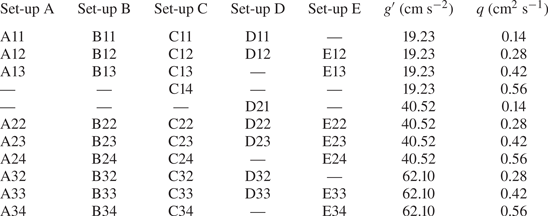
Five different permeability set-ups were examined where layer thicknesses and distributions were varied, as depicted in figure 3. The depth-averaged porosity and permeability for each set-up were calculated using (2.3) or (2.4), where  $Z_N=20$ cm was the same for all set-ups but the number of layers $N$ changed between them, as shown in figure 3 and listed in table 1. Values obtained for the depth-averaged porosity and permeability for each set-up are also listed in table 1. Approximately 7–10 gravity current experiments were conducted in each set-up and in each experiment the volume flux $q$ and fluid density $\rho _0$, or equivalently concentration $C_0$, at the source were kept constant, as recorded in table 2. In total, 42 experiments were conducted with 11 combinations of $q$ and $\rho _0$.

Figure 3. Vertical structure of the permeability in the five different set-ups discussed.
Table 1. A summary of the depth-averaged porosity  $\phi$ and permeability $k$ for each set-up. The jump factor $J$ and the image processing error $err$ are calculated using (2.21) and (3.6), respectively.

Table 2. A summary of the experiments performed in each set-up with corresponding source volume flux  $q$ and source reduced gravity $g'$, where ${g'=g(\rho _0-\rho _a)/\rho _a\equiv g\beta (C_0-C_a)}$.
3.2. Image processing and concentration maps
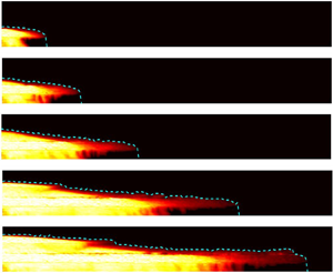
Sample gravity current images are shown in figure 4(a) for a representative experiment, A22, from table 2 for set-up A at five different times. The dashed curves shown on the individual images represent the height profiles and lengths of the gravity currents. To measure the evolving concentration, and hence the profile of these currents, we use calibrated images of the light intensity of the gravity current to measure the dye concentration. The intensity of the blue channel of the images are first subtracted at each pixel from that of the reference image. The resultant intensity matrix is then divided into vertical stripes of fixed 20–25 pixel thicknesses across the tank. For each vertical stripe we calculate the mean intensity of the column with vertical extent such that all values lie within  $1\,\%$ of the maximum intensity. This threshold defines the local height of the gravity current. The individual heights are then added to produce the height profiles. Moreover, the area engulfed by these curves is the total gravity current volume, which, after subtracting the injected volume $qt/\bar {\phi }$, gives the entrained volume $V_e$ over time $t$.
$t$.

Figure 4. Gravity current images and their concentration maps for a representative experiment A22 from table 2. Dashed curves are the height profiles of the gravity currents. Each individual panel is  $200\times 20\ {\rm cm}^2$. The colour map depicts $\hat {C}=(C-C_a)/(C_0-C_a)$.
Figure 4(b) shows the concentration maps of the respective gravity current images to the left. The concentration maps are generated to measure the spatial and temporal distributions of concentration with the help of calibration experiments that yield a functional relationship between the dye concentration and light intensity.
For the calibration experiments, the tank was uniformly saturated with the red dye in a series of concentrations
 \begin{equation} C_d = [0, 0.05, 0.10, 0.20, 0.40, 0.60, 0.80, 1.00, 1.20]\pm0.01\ \text{g}\ \text{l}^{{-}1}. \end{equation}
Images of the saturated tank were recorded with the same camera settings as discussed in § 3.1. Sample calibration curves for small and large beads are shown in figure 5, where the relative intensity,  $I_0-I$, is obtained by subtracting each image of intensity $I$ from the reference image of intensity $I_0$ in which $C_d = 0$. The calibration curves are best explained by a polynomial of the form
 \begin{equation} C_d = A (I_0-I) + B (I_0-I)^2\ \text{g}\ \text{l}^{{-}1}, \end{equation}
where  $A$ and $B$ are the polynomial fitting coefficients. To account for small variations in light intensity across the tank, we divided each calibration image into a series of $1\ {\rm cm}\times 1\ {\rm cm}$ subregions, each containing roughly $200$ pixels. For these subregions across the tank, the polynomial fitting coefficients vary within $A = 9.3\pm 0.5\times 10^{-3}\ {\rm g}\ {\rm l}^{-1}$ and $B = 8.2\pm 1.5\times 10^{-5}$. Calibration experiments were performed separately for each permeability set-up.

Figure 5. Calibration curve: dye concentration vs image intensity, with  $C_d\pm 0.01 {\rm g}\ {\rm l}^{-1}$. These curves are representatives of the calibration curves in the regions of larger or smaller size beads.
For large Péclet number (Pe) flows, it is safe to assume that the normalized dye concentration yields the normalized solute concentration (Sahu & Flynn Reference Sahu and Flynn2017)
 \begin{equation} \hat{C}=\frac{C_d}{C_{d,0}}, \end{equation}
where  $C_{d,0}$ is the reference dye concentration at the source and $\hat {C}$ is defined in (2.17). By considering $Pe=U\bar{d}/D_m$, where U is defined in (2.9), $\bar{d}$ is the mean ballotini diameter and $D_m$ is the effective molecular diffusion coefficient, we find in all our experiments $Pe\sim {O}(10^2)$, and hence we calculate the value of solute concentration using (3.5).
The concentration maps, as shown in figure 4, are obtained by inputting the values of relative intensity  $I_0-I$ of the gravity current images into (3.4) at individual subregions of size similar to that in the calibration experiments. The reference intensity $I_0$ now corresponds to the image of the tank saturated with tap water and captured just before the start of each experiment.
To check the accuracy of the post-processing schemes, we evaluate the conservation of mass (2.16) and calculate the normalized percentage error at any time  $t$ as
 \begin{equation} err = \left[\left(V_e+\frac{qt}{\bar{\phi}}\right)(\bar{C}-C_a)- \frac{qt(C_0-C_a)}{\bar{\phi}}\right]\frac{100\bar{\phi}}{qt(C_0-C_a)}, \end{equation}
where  $V_e+{qt}/{\bar {\phi }}$ is the volume inside the height profiles and $\bar {C}$ is the mean concentration obtained from the concentration maps. The error $err$ is estimated at 15 different times for each experiment. Mean errors for each set-up, for all its experiments together, are given in table 1. The overall mean error for all 42 experiments is $5.25\,\%$.
3.3. Experimental observation
In all the experiments, the thickness and permeability of the lowermost layer (depicted in figure 3) and the volume flux and reduced gravity (listed in table 2) are such that  $q>Q_c$, where $Q_c$ is the critical volume flux needed to result in an override in the second layer (Huppert et al. Reference Huppert, Neufeld and Strandkvist2013) as calculated from (1.2) with $H_L=Z_1$. Examples of the gravity current flow in a multilayered medium and the consequent overrides and Rayleigh–Taylor instabilities are shown in figure 4 for experiment A22.
In figure 4, at early time ( $t_1$) the gravity current has nearly the same length in the bottom two layers. With progress in time ( $t_2$) the override length increases and gravity-driven fingers start appearing. At intermediate time ( $t_3$) convective mixing begins in the bottom layer, while new gravity-driven fingers keep forming. In contrast, there is no override in the third layer because $k_3>k_2$. At late times ( $t_4,t_5$), while convective mixing continues in the bottom layers, a new override begins in the fourth layer because $k_4< k_3$, thus adding further to overall mixing. Apart from general convective mixing, significant longitudinal dispersion occurs, resulting in a blunt nose particularly in the second layer. Figure 4 shows that transverse and longitudinal dispersion along with the override of the gravity current is important in driving mixing.
In figure 6, the effects of injection parameters on the flow and mixing of the gravity current are compared: volume flux  $q$ in the left panels and reduced gravity $g'$ in the right panels. All parameters in the left panels have same quantitative values except $q$, likewise only $g'$ varies in the right panels. Results from the left side panels show that, with increasing $q$, the length of the override increases and the second override in the fourth layer appears more rapidly, indicating that a higher input flux enlarges the override and enhances the mixing. This consequently increases the overall gravity current length and entrained volume.

Figure 6. Concentration maps comparing the effects of volume flux (a) and reduced gravity (b) at time  $t_1=15$ min and $t_2=20$ min, respectively. Colour maps have same scales as in figure 4. Dashed curves are the height profiles of the gravity currents. Each individual panel is $200\times 20\ {\rm cm}^2$. Details of the experiments mentioned in the images are given in table 2.
In contrast, the analysis of the effects of  $g'$ in the right side panels of figure 6 show that the gravity current length is only mildly affected by $g'$, but the height is slightly larger with smaller $g'$ (A13). This results in a more prominent second override that develops gravity-driven fingers earlier than those in experiments A23 and A33. A higher degree of mixing can therefore be achieved by decreasing the source reduced gravity.
The effects of the different permeability set-ups are compared in figure 7 for the same injection parameters and times. The number of overrides in each set-up is as per the number of positive permeability jumps: three overrides each in set-ups B and D, two in set-ups A and E and only one in set-up C. The length and thickness of each override, however, depend on the respective layer thicknesses. The overrides are thicker in set-ups A and E, where highly permeable layers are relatively thicker than those in set-ups B and D. These thicker overrides enhance the longitudinal dispersion due to the blunt nose. In contrast, the magnitude of the convective mixing occurring as a result of the gravity-driven fingering depends on the thicknesses of the underlying layers of lower permeability. Therefore, the fingers are more prominent in set-up D, where the lower permeability layer is thicker, than those in set-up E, which consists of relatively thinner layers of lower permeability underneath. The variation observed in the flow patterns and subsequent mixing between the set-ups based on the concentration maps suggests that there could be a competition between the number of overriding layers and the layer thicknesses in setting the mixing rate. These effects are quantified below in § 3.4.

Figure 7. Concentration maps comparing the effects of permeability set-ups at time  $t=25$ min. Colour maps have the same scales as in figure 4. Dashed curves are the height profiles of the gravity currents. Each individual panel is $200\times 20\ {\rm cm}^2$. Details of the experiments mentioned in the images are given in table 2.
The behaviour of the gravity currents in set-up C in figure 7 is distinct from other set-ups because the bottom layer in set-up C is of higher permeability, such that there is a negative permeability jump at the first interface from the bottom. The first override occurs only in the third layer from the bottom, which, compared with other set-ups where the first override occurs in the second layer, decreases the opportunity for convective fingers and longitudinal dispersion. Therefore, a positive permeability jump is crucial for generating an overriding current and the consequent enhancement of mixing. The concentration map of set-up C in figure 7 also shows that a negative permeability jump results in a larger gravity current length but smaller height and lesser mixing.
3.4. Experimental results
Measurements obtained using the post-processing schemes described in § 3.2 from the experiments listed in table 2 are analysed below with the help of dimensionless models presented in § 2. We begin by checking the self-similarity of the measured data in their dimensional forms, then measure dimensionless coefficients and exponents for the associated power laws. These coefficients are subsequently combined with the dimensionless forms of the parameters to produce semi-empirical formulas that predict the horizontal and vertical extents of the gravity current and associated dispersive mixing with time.
For analysing the results from the experiments quantitatively, we plot the measured gravity current length ( $L$), height at the source ( $H$) and entrained volume ( $V_e$) vs time ( $t$). Sample plots are shown in figure 8 for the experiments in set-up A. We find that identical experimental data in each plot exhibit power-law behaviour in time, where the solid lines represent the power-law best fits. These suggest that the evolutions of $L$,
$L$,  $H$ and $V_e$ are self-similar in $t$. Slopes of the solid lines are the exponents to the power laws, which we calculate individually for each experiment along with their means. The mean values of the slopes from all 42 experiments for length, height and entrained volume, termed $S_L$, $S_H$ and $S_V$, respectively, are given in table 3 in index 1, where $S_L=0.70\pm 0.05$, $S_H=0.27\pm 0.04$ and $S_V=0.81\pm 0.07$ with the standard deviations of $7.40\,\%$, $16.32\,\%$ and $8.86\,\%$, respectively.

Figure 8. The log–log plots of experimental data vs time for representative set-up A: (a) gravity current length, (b) height at the source and (c) entrained volume. The solid lines are the corresponding linear fits. The slopes obtained from these fits for all set-ups together are listed in table 3 in index 1, with their standard deviations in index 2.
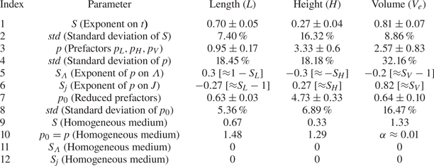
Table 3. Values of the exponents and prefactors obtained from the experiments. The exponents represent  $S=(S_{L},S_{H},S_{V})$, $S_\varLambda =(S_{\varLambda _L},S_{\varLambda _H},S_{\varLambda _V})$ and $S_j=(S_{j_L},S_{j_H},S_{j_V})$. Likewise, the prefactors represent $p= (p_L, p_H, p_V)$ and $p_0= (p_{0_L}, p_{0_H}, p_{0_V})$. In indices 9 and 10, analytical values for a homogeneous medium are given for comparison which are derived through similarity solutions (Huppert & Woods Reference Huppert and Woods1995; Sahu & Neufeld Reference Sahu and Neufeld2020), where the dispersive entrainment coefficient $\alpha \approx 0.01$. The parameters listed in indices 11 and 12 are assumed to be non-existent in case of a homogeneous medium.
Having confirmed the self-similarity of  $L$,
$L$,  $H$ and $V_e$ in $t$, we can deduce their dimensionless correlations from (2.11)–(2.13) and (2.15):
 \begin{equation} \hat{L}=p_L\hat{t}^{S_L}, \quad \hat{H}=p_H\hat{t}^{S_H}, \quad \hat{V}_e=p_V\hat{t}^{S_V}, \end{equation}
where  $p_L$, $p_H$ and $p_V$ are the dimensionless prefactors. Values of the prefactors are calculated at 8–10 equally spaced times for each experiment using the measured values, as depicted in figure 8, and the parametric values listed in tables 1 and 2. The prefactors are plotted in panels (a,b,c,) of figure 9, where each colour represents the experiments from individual set-ups from table 2. We see that the majority of the same coloured data remain nearly constant horizontally, thus verifying the self-similarity of $L$,
$L$,  $H$ and $V_e$ on $t$. The mean values of the prefactors for all 42 experiments and the standard deviations are given in table 3 in index 3 and index 4, respectively. Large standard deviations, i.e. $std>18\,\%$, in all three cases are the result of significant vertical distributions of the data between the experiments in figure 9(a–c). This implies that $p_L$, $p_H$ and $p_V$ depend on the experimental variables from table 2 – volume flux $q$ and reduced gravity $g'$ – or on the set-up parameters from table 1 – permeability $k$ and jump factor $J$.
$J$.

Figure 9. The pre factors  $p_L$ (a,d,g), $p_H$ (b,e,h) and $p_V$ (c,f,i) obtained from (3.7a–c) are plotted against time $t$ in (a–c) for all experiments with approximately 10 equi-spanned times from each experiment. (d–f) The mean values of $p_L$, $p_H$ and $p_V$ for each experiment are normalized with the dimensionless variable $\varLambda$ from (2.20) and exponents $S_{\varLambda }$ $(S_{\varLambda _L},S_{\varLambda _H},S_{\varLambda _V})$ from table 3 and plotted against $\varLambda$, where specific colours represent the experiments from the same set-up. (g–i) Show the constants $p_0$
$p_0$  $(p_{0_L}, p_{0_H}, p_{0_V})$ from (3.9a–c) which also depict the convergence obtained in $p$ after considering the effects of the jump factor $J$, whose values are taken from table 1 for each set-up. The mean values of $p_0$ and their standard deviations for all 42 experiments for each parameter $(L,H,V_e)$ are listed in table 3 in index 7 and index 8.
We employ the dimensionless variable  $\varLambda ={q\nu }/{g'k^{3/2}}$, defined in (2.20), to find the dependence of $p_L$, $p_H$ and $p_V$ on the injection parameters and medium properties. The prefactors from panels (a,b,c) of figure 9 are averaged over time for each experiment and analysed against $\varLambda$. We find that the correlations are best fit by the power laws
 \begin{equation} p_L \propto \varLambda^{S_{\varLambda_L}} , \quad p_H\propto \varLambda^{S_{\varLambda_H}} , \quad p_V\propto \varLambda^{S_{\varLambda_V}}, \end{equation}
with the slopes  $S_{\varLambda _L}=0.3$, $S_{\varLambda _H}=-0.3$ and $S_{\varLambda _V}=-0.2$. The results are shown in panels (d,e,f) of figure 9, where individual circles represent each experiment and identically coloured groups represent each set-up. The prefactors from each set-up are segregated vertically, indicating that the prefactors vary between the set-ups but are constant within each set-up. The segregation is found to be more prominent for the entrained volume than those for the length and height of the currents.
To account for the effects of permeability structure, we introduce the dimensionless jump factor  $J$ from (2.21) into the prefactors. We take the mean of the prefactors for each set-up from the middle panels in figure 9 and analyse them against the values of $J$ from table 1. The best fitted data are presented in panels (g,h,i) of figure 9, where the prefactors now promisingly coincide with the constant lines represented by $p_{0_L}=0.63$, $p_{0_H}=4.73$ and $p_{0_V}=0.64$, respectively, in the left, middle and right panels. The prefactors from (3.8a–c) can therefore be expanded as
 \begin{equation} p_L = p_{0_L}\varLambda^{S_{\varLambda_L}}J^{S_{j_L}}, \quad p_H = p_{0_H}\varLambda^{S_{\varLambda_H}}J^{S_{j_H}}, \quad p_V = p_{0_V}\varLambda^{S_{\varLambda_V}}J^{S_{j_V}}, \end{equation}
where the values of the exponents  $S_{\varLambda _L}$, $S_{\varLambda _H}$ and $S_{\varLambda _V}$ and $S_{j_L}$, $S_{j_H}$ and $S_{j_V}$ and constants $p_{0_L}$, $p_{0_H}$ and $p_{0_V}$ are listed in table 3 in indices 5, 6 and 7, respectively.
In index 8 of table 3, the standard deviations of the constants  $p_{0_L}$, $p_{0_H}$ and $p_{0_V}$ are given, which are $std<7\,\%$ for the former two and $std<17\,\%$ for the latter. These values, in comparison with the standard deviations of $p_{L}$, $p_{H}$ and $p_{V}$ in index 4, show significant improvement. This is also in line with the agreement we see in panels (g,h,i) of figure 9 compared with that in panels (a,b,c).
3.5. Semi-empirical models
A straightforward substitution of (3.9a–c) into (3.7a–c) gives
 \begin{equation} \hat{L}=p_{0_L}\varLambda^{S_{\varLambda_L}}J^{S_{j_L}}\hat{t}^{S_L}, \quad \hat{H}=p_{0_H}\varLambda^{S_{\varLambda_H}}J^{S_{j_H}}\hat{t}^{S_H}, \quad \hat{V}_e=p_{0_V}\varLambda^{S_{\varLambda_V}}J^{S_{j_V}}\hat{t}^{S_V}. \end{equation}
Now, the conversion of the dimensionless  $\hat {L}$, $\hat {H}$ and $\widehat {V_e}$ in (3.10a–c) into their dimensional forms with the help of (2.9)–(2.13), (2.15) and (2.20) yields the gravity current length, height and entrained volume
 \begin{gather} L=p_{0_L}J^{S_{j_L}}q^{(1-S_L+S_{\varLambda_L})}\bar{k}^{(2S_{L}-1-3S_{\varLambda_L}/2)}\left(\frac{g'}{\nu}\right)^{(2S_L-1-S_{\varLambda_L})}\left(\frac{t}{\bar{\phi}}\right)^{S_L}, \end{gather}
 \begin{gather}H= p_{0_H}J^{S_{j_H}}q^{(1-S_H+S_{\varLambda_H})}\bar{k}^{(2S_{H}-1-3S_{\varLambda_H}/2)}\left(\frac{g'}{\nu}\right)^{(2S_H-1-S_{\varLambda_H})}\left(\frac{t}{\bar{\phi}}\right)^{S_H}, \end{gather}
 \begin{gather}V_e = p_{0_V}J^{S_{j_V}}q^{(2-S_V+S_{\varLambda_V})}\bar{k}^{(2S_{V}-2-3S_{\varLambda_V}/2)}\left(\frac{g'}{\nu}\right)^{(2S_V-2-S_{\varLambda_V})}\left(\frac{t}{\bar{\phi}}\right)^{S_V}. \end{gather}
The experimental values of the constants  $p_0$ and exponents $S_j$, $S_\varLambda$ and $S$ for all three parameters ( $L,H,V_e$) for the heterogeneous set-ups examined here are listed in table 3.
On considering the effects of  $J$ and $\varLambda$ on $L$,
$L$,  $H$ and $V_e$, we find that $S_j$ and $S_\varLambda$ are numerically but approximately related to $S$ for all three parameters, as described in indices 5 and 6 of table 3. Therefore, for further simplification of (3.11)–(3.13), we consider the values of $S_\varLambda$ and $S_j$ from the square brackets in table 3 as ( $S_{\varLambda _L}\approx 1- S_L$, $S_{\varLambda _H}\approx -S_H$, $S_{\varLambda _V}\approx S_V-1$) and ( $S_{j_L}\approx S_L-1$, $S_{j_H}\approx S_H$, $S_{j_V}\approx S_V$). These substitutions give us approximate expressions for the gravity current length, height and entrained volume from (3.11)–(3.13) with a single exponent type, i.e. $S_L$, $S_H$ or $S_V$, on each term instead of three:
 \begin{gather} L\approx\frac{p_{0_L}}{J^{1-S_{L}}}q^{(2-2S_L)}\bar{k}^{(7S_{L}-5)/2}\left(\frac{g'}{\nu}\right)^{(3S_L-2)}\left(\frac{t}{\bar{\phi}}\right)^{S_L}, \end{gather}
 \begin{gather}H\approx p_{0_H}J^{S_{H}}q^{(1-2S_H)}\bar{k}^{(7S_{H}-2)/2}\left(\frac{g'}{\nu}\right)^{(3S_H-1)}\left(\frac{t}{\bar{\phi}}\right)^{S_H} , \end{gather}
 \begin{gather}V_e\approx p_{0_V}J^{S_{V}}qk^{(S_{V}-1)/2}\left(\frac{g'}{\nu}\right)^{(S_V-1)}\left(\frac{t}{\bar{\phi}}\right)^{S_V}. \end{gather}
We plot the empirical models from (3.14)–(3.16) against  $t$ in their dimensionless forms in figure 10 with the measured values of $L$,
$L$,  $H$ and $V_e$, where the dimensionless forms are obtained from (3.10a–c) with the approximate values of $S_\varLambda$ and $S_j$ described above. We see good agreement in all cases between the empirical model and measured values.

Figure 10. Experimental data and the best fits vs time  $\hat {t}$: (a) gravity current length $\hat {L}$, (b) height at the source $\hat {H}$, (c) entrained volume $\hat {V}_e$ and (d) mean concentration $\hat {C}$. The best fit solid lines are obtained from (3.14)–(3.16) and (3.18) by converting them into the dimensionless forms.
Figure 10(d) shows the comparison of the mean concentration of the gravity current, where the experimental values are obtained from the concentration maps and the empirical model is obtained from the mass conservation (2.19) with the help of (3.7a–c) and (3.9a–c):
 \begin{equation} \hat{C} = \frac{1}{1+p_{0_V}J^{S_{j_V}}\varLambda^{S_{\varLambda_V}}\hat{t}^{(S_V-1)}}. \end{equation}
Using the approximations of  $S_{\varLambda _V}$ and $S_{j_V}$ similar to those used in (3.16), and the expansions of $\hat {C}$, $\hat {t}$ and $\varLambda$ using (2.17), (2.11) and (2.20), provide an estimate of the mean concentration
 \begin{equation} \bar{C} \approx C_a+\left[\frac{(C_0-C_a)}{1+p_{0_V}J^{S_{V}}\left(\dfrac{ k^{1/2}g'}{\nu\phi}\right)^{(S_V-1)}t^{(S_V-1)}}\right]. \end{equation}
Unlike the length, height and entrained volume of the gravity current, the mean concentration in figure 10 does not follow a power law in time because it is constrained by the limits  $0\leqslant \hat {C}\leq 1$. The agreement in this case is not excellent because the measurement of concentration involves the use of concentration maps, which have a mean error of 5.25 %, as discussed in § 3.2. The image processing error gets added up with the errors in the empirical modelling, i.e. large standard deviations of 8.86 % and 16.47 % of $S_{V}$ and $p_{0_V}$, respectively, resulting in only modest agreement.
4. Discussion
The empirical models reported here for the length, height and entrained volume of a gravity current in a heterogeneous porous medium are given in (3.11)–(3.13), along with their simplified approximate forms in (3.14)–(3.16). The empirical values of the constants and exponents for the heterogeneous set-ups examined here are listed in table 3, along with the theoretical values for the case of a homogeneous medium.
On comparing the model presented in (3.11)–(3.13) with that of Huppert & Woods (Reference Huppert and Woods1995) and Sahu & Neufeld (Reference Sahu and Neufeld2020) for homogeneous media, we find that  $L$,
$L$,  $H$ and $V_e$ do not depend on the dimensionless parameter $\varLambda$. Moreover, from (2.21), the jump factor $J=1$ for homogeneous media. Therefore, for a homogeneous medium, it is safe to assume that $(S_\varLambda,S_j)=(0,0)$. By substituting the values of the exponents and prefactors for the homogeneous case from indices 9 and 10 of table 3 ( $S_L=0.67$, $S_H=0.33$, $p_{0_L}=1.48$, $p_{0_H}=1.29$) and $(S_\varLambda,S_j)=(0,0)$ into (3.11) and (3.12), the similarity solution of Huppert & Woods (Reference Huppert and Woods1995) for the length and height of the gravity current can be recovered. Likewise, by substituting $S_V=1.33$ and $p_{0_V}=0.01$ into (3.13), the semi-empirical solution of Sahu & Neufeld (Reference Sahu and Neufeld2020) for the entrained volume is recovered.
Sahu & Neufeld (Reference Sahu and Neufeld2020) suggest that the magnitude of entrainment of the ambient fluid into the gravity current depends on a term called the dispersive entrainment coefficient, which is equivalent to the dimensionless dispersivity in a homogeneous medium. They anticipate that, due to flow instabilities and local velocity gradients in a heterogeneous porous medium, the dispersive entrainment is significantly higher and therefore the effective dispersive entrainment coefficient is much larger in a heterogeneous medium than in a homogeneous medium. We verify this anticipation in the current study. The values of  $p_V(2.57,0.01)$ given in indices 3 and 10 in table 3 are the equivalent dispersive entrainment coefficients in heterogeneous and homogeneous media, respectively. The values suggest that the effective dispersive entrainment coefficient in heterogeneous media is approximately 250 times greater than in homogeneous media at early times for the same depth-averaged medium properties and injection parameters. This result implies that the amount of mixing in a heterogeneous medium can be higher by several orders of magnitude than that in a homogeneous medium depending on the type of heterogeneity.
Sahu & Neufeld (Reference Sahu and Neufeld2020) also predict that the length of the current and the height at the source are unaffected by the heterogeneity or the amount of mixing. The experimental results from the current work, however, show otherwise.
For the heterogeneous set-ups examined here, the exponent  $S_L=0.70$ is larger and $S_H=0.27$ and $S_V=0.81$ are smaller than those for homogeneous media (0.67, 0.33, 1.33). In contrast, prior to considering the effects of $J$ and $\varLambda$, from index 3 of table 3, the prefactors $p_L=0.95$ is smaller and $p_H=3.33$ and $p_V=2.57$ are larger than their equivalents for a homogeneous medium (1.48, 1.29, 0.01). For power-law behaviour, the value of the prefactor dictates the magnitude of the parameters at early times, whereas the exponent dominates at late times. Therefore, for the set-ups examined here, the empirical values reported here suggest that the gravity current height, similar to the entrained volume, is larger at early times in a heterogeneous medium than that in a homogeneous medium for comparable values of depth-averaged permeability, porosity and injection parameters. A reverse of this behaviour is found for the gravity current length.
The enhanced mixing at early times due to the heterogeneity rapidly decreases the concentration of the injected fluid. The lighter density of the mixed fluid compared with that originally injected subsequently results in an easier vertical buoyant motion, instead of horizontal propagation. Due to the reduced horizontal velocity of the gravity current, the effects of longitudinal dispersion start dominating the longitudinal advection. This decreases the concentration of the current further. The rapid decrease in the concentration results in a thicker gravity current, which tends to violate the assumption of a long and thin current that is crucial for satisfying the hydrostatic pressure assumption and the neglect of the vertical velocity gradient in the current.
Most of the gravity current models derived by previous researchers assume that the gravity current is long and thin, but the enhanced mixing due to the heterogeneity tends to violate this assumption much earlier than the period for which a solution of the late time regime is applicable. In a late time regime, it is therefore crucial to consider the vertical velocity in the current and model it as a two-dimensional problem.
5. Summary and conclusions
By recognizing the role of heterogeneity in the permeability of the medium in dictating the flow and mixing within porous media, we have presented results and analysis based on laboratory experiments to characterize the behaviour of gravity currents in multi-layered porous media. The experimental set-up consisted of multiple parallel layers of various permeability, which were obtained with the help of different sizes of spherical glass ballotini. The working fluids for the experiments were fresh water and dense salt water. The permeability ratios and the combinations of the layers, their thicknesses and the flow rate and solute concentration at the injection were considered the flow variables in the analysis. Based on the types of the structures, we also introduced a term called the ‘jump factor’, which quantifies the potential of layered structure towards mixing.
Our experiments show that mixing between the gravity current and ambient fluid gets amplified due to the layered structures. For a similar set of depth-averaged parameters, e.g. porosity and permeability, and flow conditions, e.g. volume flux and concentration, the mixing in a layered heterogeneous medium could be as large as 250 times than that in the homogeneous medium. Equivalently, the dispersive entrainment coefficient  $\alpha \approx 2.57$ in a heterogeneous medium could be of ${O}(2)$ greater than that for a homogeneous medium, i.e. $\alpha \approx 0.01$ as predicted by Sahu & Neufeld (Reference Sahu and Neufeld2020). We also find, for a similar set of variables, that the height of the current is greater in a heterogeneous medium than that in a homogeneous medium, whereas the gravity current length is smaller.
Because of large dispersion into the gravity current at early times, the gravity currents become blunt, which further enhances the possibility of longitudinal dispersion. This leads to a thick current with a blunt nose. Therefore, the assumption of long and thin current that is central to modelling the gravity current flow theoretically is generally invalid after a certain time scale.
Based on the experimental findings and dimensionless modelling, we present semi-empirical formulas that predict the height and length of the gravity current and entrained volume into the gravity current as a function of time and other parameters. These three parameters monotonically increase, however, simultaneously, the mean concentration of the current decrease with time, which is also predicted in this work.
The experimental results and semi-empirical models from the current work can be used to predict the behaviour of gravity current flow and mixing in a heterogeneous medium of much larger length scale by appropriately defining the depth-averaged parameters and jump factors. The experimental images can be used for the validation of a computational model built for modelling flows in a highly heterogeneous system.
Some obvious drawbacks of the current work are the well-defined parallel layers and large permeability and porosity values, which do not necessarily simulate a real geological rock. As a next step of this work, it would be useful to consider varied combinations of layers, for example with inclined interfaces between them. The experimental work may be extended to numerical modelling where more realistic values of porosity and permeability can be considered. Finally, the Rayleigh–Taylor instabilities may be investigated mathematically to predict the mixing due to the gravity-driven fingers more accurately.
Funding
This research is a contribution from the GeoCquest consortium, a BHP-supported collaborative project between the Universities of Cambridge, Stanford and Melbourne.
Declaration of interests
The authors report no conflict of interest.


 Open access