


1. Introduction
Fluid mixing by turbulent bubble plumes is used in many industrial and environmental situations, including the water reservoirs for preventing algal blooms (Neto, Cardoso & Woods Reference Neto, Cardoso and Woods2016) and reaction vessels to drive hydrogenation reactions (cf. Deckwer & Field Reference Deckwer and Field1992; Joshi et al. Reference Joshi, Vitankar, Kulkarni, Dhotre and Ekambara2002). The dynamics of such bubble plumes is also key for assessing risks of methane clathrate release (Duarte et al. Reference Duarte, Lenton, Wadhams and Wassmann2012) and  ${\rm CO}_2$-driven lake overturning, such as at Lake Nyos, Cameroon (Woods & Phillips Reference Woods and Phillips1999). Furthermore, the dynamics of turbulent multiphase bubble plumes is relevant for modelling the fate of oil and gas produced during blowout events in the deep sea (Socolofsky, Adams & Sherwood Reference Socolofsky, Adams and Sherwood2011).
There is a long history of laboratory experiments which have explored the dynamics of bubble plumes and recognised a number of different flow regimes. A common feature of bubble plumes is the relatively large slip velocity of the bubbles. This tends to result in bubble–fluid separation, and hence a considerably more complex dynamics than their single-phase turbulent plume counterparts (Morton, Taylor & Turner Reference Morton, Taylor and Turner1956). Experiments have been reported in both uniform and density-stratified ambient fluid, and a hierarchy of different models have been presented based on observations of the bubble and fluid trajectories in the flow.
In an early modelling paper, Mcdougall (Reference Mcdougall1978) described the plume in terms of a central core of large bubbles, with slip, and an outer core of smaller bubbles and entrained fluid, building from the classical picture of a single-phase turbulent plume. However, as the bubble size increases, it has become clear that, as well as the effect of slip, bubble distortion, break up and even coalescence can be important elements in the flow dynamics (e.g. Milgram Reference Milgram1983; Leitch & Baines Reference Leitch and Baines1989). In some studies of bubble plumes in a uniform ambient, the classical model for a single-phase buoyant plume has been used as a reference, although the multiphase flow system is more complex. With a single-phase plume, the flow is well characterised in terms of the total buoyancy flux  $B$, leading to the prediction that the radius increases linearly with height $z$, while the fluid velocity $u$ gradually falls off as
 \begin{equation} u=k_1 B^{1/3} z^{-1/3} \end{equation}
and the volume flux  $Q$ increases as
 \begin{equation} Q=k_2 B^{1/3} z^{5/3} , \end{equation}
where  $k_1=(5/6\alpha )(9\alpha /10)^{1/3}\approx 3.7$ and $k_2=(6 \alpha {\rm \pi}/5)(9\alpha /10)^{1/3}\approx 0.15$ are two constants dependent on the entrainment coefficient $\alpha$ (Morton et al. Reference Morton, Taylor and Turner1956). Provided that the plume velocity exceeds the bubble slip velocity, $u\gg v_s$, then this model has been shown to be successful in describing the dynamics of a bubble plume. However, when $u\leqslant 0.4 v_s$, which occurs sufficiently far from the source, $z\gg 2 B/v_s^3$ (see (1.1); cf. Leitch & Baines Reference Leitch and Baines1989; Socolofsky & Adams Reference Socolofsky and Adams2005; Lai & Socolofsky Reference Lai and Socolofsky2019; Wang, Lai & Socolofsky Reference Wang, Lai and Socolofsky2019), experiments show that bubble slip has a key role in the transport (Chen & Cardoso Reference Chen and Cardoso2000; Wang et al. Reference Wang, Lai and Socolofsky2019).
Leitch & Baines (Reference Leitch and Baines1989) carried out some small-scale bubble plume experiments, and showed that when the bubble slip velocity exceeds the plume velocity, the plume radius increased with height  $z$ at a rate proportional to $z^{1/2}$ while the volume flux in the plume increased linearly with height. Recently, some very high-resolution data have been presented by Lai & Socolofsky (Reference Lai and Socolofsky2019) and Wang et al. (Reference Wang, Lai and Socolofsky2019) on the dynamics of bubble plumes in a large 10 m experimental facility, in which the plume properties were measured at 5 different heights in the flow. In accord with Leitch & Baines, Lai & Socolofsky also found that the radius of the plume tends to grow with the square root of the height, but they propose a different model for the variation of volume flux with height. Wang et al. (Reference Wang, Lai and Socolofsky2019) also argue that bubble dispersion has an important role in the dynamics.
Here, we build on these earlier studies and present a series of new small-scale laboratory experiments in which we use dye visualisation techniques to track the motion of both the bubbles and the fluid continuously with height in such a ‘slip plume’, where the bubble speed far exceeds the speed of the equivalent single-phase turbulent buoyant plume. From these data, we establish some new constraints on the time-averaged radius and fluid speed. We also assess the volume flux in the plume using the filling box method (cf. Leitch & Baines Reference Leitch and Baines1989). In our experiments, the bubbles have size of order 1–10 mm and so the rise speed lies in the range  $0.2\unicode{x2013}0.3\ {\rm ms}^{-1}$. The plume speed typically falls below the bubble speed within a few cm of the source. In order to explore the transition from the classical plume flow to the slip-controlled regime, we therefore also report some additional particle-plume experiments, using particles with much smaller slip speed than the bubbles. In these particle-plume experiments, a suspension of heavy particles in fresh water is used to form a descending plume. We find directly analogous results for the particle plumes once in the slip regime, but now the transition to the slip regime occurs further from the source. We identify a scaling for the transition distance from the near-source classical turbulent plume to the far-field slip-dominated plume. The length scale for this transition scales with $\lambda^{3/2} B/v_s^3$, where $B/v_s^3$ corresponds to the length scale of two-phase plumes proposed by Bombardelli et al. (Reference Bombardelli, Buscaglia, Rehmann, Rincón and Garcia2007), and relates to the length scales proposed by earlier authors (cf. Wilkinson Reference Wilkinson1979; Milgram Reference Milgram1983; Leitch & Baines Reference Leitch and Baines1989; Baines & Leitch Reference Baines and Leitch1992; Aseada & Imberger Reference Aseada and Imberger1993; Socolofsky & Adams Reference Socolofsky and Adams2005). However, in § 7 we identify that the parameter $\lambda$ depends on the Reynolds number of the particles. A key contribution of our experiments is to demonstrate a change in the overall behaviour of the plume at this point, as the bulk plume speed falls below the slip speed of the bubbles; beyond this point, the flow becomes dominated by the bubble slip, rather than the dynamics of a single-phase buoyant plume. We discuss the importance of our results for the mixing and transport in multiphase plumes, and delineate conditions under which the different regimes apply.
2. Experimental system
A number of bubble plume experiments were carried out in a Perspex tank, of size  $60 \times 60 \times 80$ cm, filled with fresh water, using a peristaltic pump to supply a steady flux of bubbles from a nozzle located at the centre of the floor of the tank (figure 1a). Three series of experiments were carried out using three nozzle designs, resulting in bubbles of different sizes (nozzle designs A–C, see table 1, figure 2(a) and Appendix A). A fourth series of experiments (herein denoted by D) was carried out using the same nozzle as in experiments C; however, in this fourth series of experiments, the water in the tank was mixed with a small volume of surfactant, and this led to a reduction in the mean bubble size (see table 1, figure 2(a) and Appendix A). For each series of experiments, the gas flux $Q_b$ was systematically varied from 1.1 to $21.1\ {\rm cm}^3\ {\rm s}^{-1}$. Table 1 details the source conditions and the values of various properties measured in each experiment.

Figure 1. Schematics illustrating the different set-ups of (a) the bubble and (b) the particle-plume experiments.

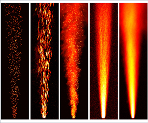
Figure 2. (a) Images of four different bubble plumes with identical gas flux  $Q_b$ but different nozzle design, resulting in bubbles of different sizes. (b) Bubble size frequency distribution for the different plumes depicted in (a). (c) Mean bubble diameters as a function of the source buoyancy flux, for a number of experiments in table 1.
Table 1. Conditions of the bubble plume experiments. Here,  $Q_b$ is the source gas flux, $d$ the mean diameter of the bubbles, $v_s$ the mean bubble slip velocity, $u_l$ the mean fluid velocity in the plume and $t_0=\rho d^2/18\mu$ is the Stokes relaxation time for a bubble of size $d$, with $\rho$ the density of the particles.

A LightTape light panel (Electro-LuminX Lighting Corp.) was connected to the rear of the tank and provided uniform illumination. On the opposite side, a Nikon D5300 RGB digital camera was used to record the whole duration of each experiment with full-HD resolution and a frame rate of 60 Hz, while a Spark SP-5000M-USB camera with a faster frame rate of 400 Hz was used to record high-frequency footage of the rising bubbles and fluid.
In each experiment, a small flux of clear, neutrally buoyant water was continuously pumped into the nozzle with the air. Over the course of the experiment, pulses of dye could be added to this water, without affecting the source flow, to observe the motion of the water as it rises in the plume. A number of filling box experiments were carried out, for which the fluid initially in the tank had some salt added (NaCl concentration of order 0.5 %–1.0 %), except for a thin layer of dyed, fresh water which was placed above the top of the saline solution (see figure 7). As the flow developed, the water carried up by the bubble plume spread out into this upper layer of fresh water. By tracking the depth of the interface between the dyed, fresher water in the upper part of the tank and the clear saline water underneath, we could estimate the upward flux of water in the plume as it passes the interface.
As discussed in § 7, a series of particle-plume experiments were also carried out to complement the results of the bubble plume experiments. The particle experiments were carried out using the same experimental apparatus as the bubble experiments, but the nozzle was now located at the top of the tank rather than the bottom (see figure 1(b) and Appendix A). In these experiments, a suspension of silicon carbide particles (Washington Mills) in fresh water was supplied through the nozzle and formed a descending particle plume in the tank. Particles of different sizes were used in different experiments, with the mean particle diameter ranging between 12.8 and  $203.0\ \mathrm {\mu }{\rm m}$. The density of the silicon carbide particles was $\rho _p=3.217\ {\rm g}\ {\rm cm}^{-3}$. The conditions of the particle experiments are listed in table 2.
Table 2. Conditions of the particle-plume experiments. Here,  $Q$ is the source volume flux, $g'$ is the reduced gravity of the suspension of particles in fresh water at the source, $B$ is the buoyancy flux, $d$ is the mean diameter of the particles, $v_s$ is their settling velocity and $t_0=\rho d^2/18\mu$ is the Stokes relaxation time for a particle of size $d$.
$d$.

For a number of particle plumes, a filling box experiment was also carried out using the same approach as discussed above. In these experiments, however, a small amount of dye was added to a thin layer of saline fluid located at the base of the tank, while the upper layer of fresh water was clear (see figure 8). As the particle plume transported liquid to the base of the tank, the height of the interface separating the upper layer of clear fluid from the lower layer of dyed fluid progressively increased over the course of an experiment. By tracking this increasing height as a function of time, we estimated the downward flux in the particle plume as a function of distance from the source.
3. Experimental observations
In figure 2(a), we present four instantaneous images of the bubble plumes which developed in four experiments with identical gas flux  $Q_b$, but different nozzle designs (experiments 5, 17, 29 and 40 in table 1). Nozzle A resulted in larger, less frequent bubbles, while nozzles B–D produced increasingly small, frequent bubbles for any given gas flux.
In each experiment, the bubbles in the plume had a narrow range of sizes. This may be seen in a typical histogram showing the bubble size distribution obtained by measuring the size of the bubbles in one photograph of the plume, as captured by the high-speed camera (figure 2b). For non-circular bubbles, the diameter of the equivalent circular bubble having the same surface area was estimated. Applying a similar analysis to images from each experiment, we have been able to estimate the mean bubble size in each experiment. The data shown in figure 2(c) illustrate that the bubble sizes are nearly constant for a given nozzle and depend on the presence or not of surfactant in solution, but are largely independent of the bubble flux.
Although the size and the spacing between the bubbles were different across the four series of experiments, we note that in each case, the flow gradually appeared to broaden out with distance from the source (see figure 3a). In all experiments, the bubbles meandered while rising through the tank. Figure 3(b), which was obtained by averaging 50 consecutive frames captured by the high-speed camera during a typical experiment, illustrates the path of the rising bubbles. In this figure we observe that there is no evidence of large-scale turbulent structures or eddies in the plume: this suggests that the slip plume dynamics and entrainment process are different to those in a classical single-phase buoyant plume (Morton et al. Reference Morton, Taylor and Turner1956).

Figure 3. (a) Instantaneous image of the bubbles in a typical experiment (no. 26 in table 1), shown in false colour. (b) Illustration of the trajectories followed by the bubbles as they ascend through the tank, obtained by averaging 50 consecutive frames. (c) Instantaneous image of the plume containing dyed fluid. (d) Time-averaged distribution of the bubbles in the plume, obtained by averaging the frames captured during the first part of the experiment, during which the plume fluid is clear. (e) Time-averaged distribution of the ascending fluid in the plume, obtained by averaging the frames captured during the second part of the experiment, during which the plume fluid is dyed.
Part way through each experiment, neutrally buoyant dye was added to the plume fluid at the source. The dyed fluid was transported upwards by the bubbles in the plume, as illustrated in figure 3(c), which corresponds to the bubbles shown in figure 3(a). In figures 3(d) and 3(e), we present two time-average images. Figure 3(d) was obtained by averaging the frames captured during the first part of the experiment, in which the plume fluid was clear; in this image, false colours are used to illustrate the time-averaged light attenuation produced by the bubbles in the plume. Figure 3(e) was obtained by averaging the frames captured during the second part of the experiment, when the plume fluid was dyed. Here, the colours illustrate the time-averaged light attenuation produced by the dyed fluid in the plume.
For each experiment, we used the time-average figures to locate the time-averaged edges of the plume, defined as the locus of the points which have a light attenuation relative to the background equal to  $1/e$ of the light attenuation at the centre of the plume relative to the background. As an example, in figure 4(a), we use red circles to plot the time-averaged radius of the bubbles in a typical bubble plume, $r_b$, as a function of distance above the source (experiment 30 in table 1); while we use blue circles to plot the time-averaged radius of the ascending dyed fluid in the same experiment, $r_l$, again as a function of height. This analysis has been carried out for all the experimental plumes.

Figure 4. (a) Time-averaged radius of the bubble and of the liquid as a function of height above the source (experiment 30 in table 1). (b) The plume radius  $r_b$ grows with the square root of distance from the source, $z$. (c) The values of $k_b$ used to collapse the profiles in (b) are plotted as a function of the buoyancy flux $B$. (d) The ratio $r_l/r_b$ is plotted for a number of experiments as a function of $B$.
$B$.
In the slip plume regime, we expect that the properties of the flow depend on the buoyancy flux,  $B$, the rise speed of the bubbles, $v_s$, and the distance from the source, $z$. Analysis of the experimental data suggests that the radius increases with $z^{1/2}$, and so by dimensional analysis, we expect that
 \begin{equation} r_b = k_b \left(\frac{Bz}{v_s^3}\right)^{{1}/{2}}. \end{equation}
In figure 4(b), we plot  $r_b$ as a function of $k_b (Bz/v_s^3)^{1/2}$, where for each experiment, $k_b$ is chosen to give the best fit to expression (3.1). In figure 4(c), we then illustrate the values of $k_b$ used to obtain this best fit as a function of $B$. It is seen that, to good approximation, the data in figure 4(b) follow a straight line, consistent with the model (3.1). In figure 4(c), the data points are coloured blue, red, yellow and green for the four different bubble sizes (see table 1 and figure 2). Although there is some scatter, figure 4(c) indicates that $k_b$ is approximately constant in our experiments, and the best fit value for $k_b$ is $k_b = 2.38\pm 0.45$.
Using the relation  $r_i = k_i(Bz/v_s^3)^{1/2}$ for both the bubble, $i=b$, and the liquid, $i=l$, radii, we compare the radius of the bubble and liquid plumes as a function of $B$ in figure 4(d). It is seen that for each bubble size, the ratio of radii is essentially constant, increasing with bubble size. This means that in slip plumes with larger bubbles, the liquid spreads over a larger radius than the bubbles, while in slip plumes with smaller bubbles the bubble and the liquid radii are closer in magnitude.
4. Speed of bubbles and liquid in the slip plume
Our measurements suggest that the bubbles have a near constant upward speed with height. This may be seen in figure 5, in which we show a time series of a vertical line of pixels through the centre of the plume. There are a series of inclined thin lines on the left-hand side of the figure, corresponding to the ascent of individual bubbles. These are of nearly constant and equal slope, parallel to the thick red dotted line in figure 5. Some time after the start of the experiment, the source fluid was dyed, and the yellow–red streaks on the right-hand side of figure 5 represent the ascent of this dyed source fluid. Although there is more variability in the speed of this fluid, using the Hough transform to detect changes in the light intensity, and hence the dye streaks, we can determine the slope of these lines with accuracy of  $\pm 10\,\%\unicode{x2013}15$ % (Lippert & Woods Reference Lippert and Woods2018; Mingotti & Woods Reference Mingotti and Woods2016, Reference Mingotti and Woods2019). Figure 5 shows that the speed of the ascending liquid along the centreline of the plume is much smaller than that of the bubbles, and appears to be nearly uniform over the height range of the experiment, of approximately 70 cm.

Figure 5. Time series of a vertical line of pixels along the plume centreline in experiment 27 (see table 1), showing the different velocities at which the bubbles and the liquid rise in the plume.
Using a number of time series images equivalent to that shown in figure 5, we have measured the profiles of bubble and liquid velocity along the plume centreline as a function of height above the source in each experiment. Figure 6(a) illustrates the results of our measurements for a number of plumes issuing from nozzle C, which are characterised by bubbles of mean size 2.5 mm (see table 1). It is seen that after some initial adjustment in the near-source region, the bubble rise speed  $v_s$ is approximately constant with height for a given nozzle and hence bubble size (cf. table 1). The speed of the liquid along the centreline of the plume is also approximately constant with height, and the ratio between the liquid speed and the bubble speed along the plume centreline is approximately $v_l/v_s=0.30\pm 0.03$ in all our experiments (see figure 6b).

Figure 6. (a) Bubble and liquid velocity measurements as a function of height above the source along the centreline in a number of experiments (see table 1). (b) Ratio between the liquid and the bubble centreline velocities,  $v_l/v_s$, as a function of the buoyancy flux, $B$. (c) Bubble and liquid velocity measurements taken at four different heights above the source, $z/H$, and at various radial distances from the centreline, $x/r_l$, in a plume containing large bubbles (experiment 6, see table 1). (d) Bubble and liquid velocity measurements taken at the same heights and radial distances from the centreline as in (c), but in a plume containing smaller bubbles (experiment 30 in table 1).
We have also analysed additional time series equivalent to that shown in figure 5 but measured at different radial positions across the plume, in order to measure the fluid and bubble velocities in each experiment as a function of radial distance from the centreline, as well as height. These data are shown in figures 6(c)–6(d) for two plumes issuing from nozzles (c) A and (d) C, which are characterised by bubbles of mean size (c) 10 mm and (d) 2.5 mm. The figures illustrate that the bubble speed is maximum along the centreline of the plume, and decreases slightly across its width. The maximum velocity of the liquid within the bubble radius is approximately 1/3 of the corresponding bubble speed, as noted above, but beyond the bubble radius, the liquid speed falls to much smaller values, close to zero. This picture of the bubble plume shows that bubble slip is a critical feature of the flow throughout the plume over the parameter range of this experimental study.
5. Volume flux in the slip plume
In order to measure the volume flux in the slip plumes, we ran a series of filling box experiments in which a two-layer stratification was set up in the tank, with a layer of clear, weakly saline fluid below a thin layer of red fresh water. As the bubble plume developed, it transported a volume of fluid upwards in the tank, and this led to a downflow in the ambient fluid. Figure 7(a) shows a series of photographs which were captured at regular time intervals during a typical experiment. It is seen that the interface between the clear and dyed fluid remained sharp over the course of the experiment.

Figure 7. (a) Series of images captured at regular time intervals during a typical filling box experiment. (b) Time series of the horizontally averaged vertical profile of dye concentration in the tank. (c) Fractional height of the interface between the dyed upper layer fluid and the clear lower layer fluid as a function of time, for four typical experiments with bubbles of different sizes (experiments 6, 18, 30 and 41, see table 1). (d) Coefficient  $\lambda$ (see (5.2)–(5.4)) plotted as a function of the buoyancy flux $B$.
$B$.
In figure 7(b), we present a time series of the horizontally averaged vertical profiles of dye concentration in the tank, which shows the descent of the fluid front during the experiment. It is seen that the flow gradually slows down as the front approaches the base of the tank.
If we plot the logarithm of the height of the interface,  $\log (z)$, as a function of time, $t$, we find that for each experiment, the data follow a straight line. In figure 7(c) we illustrate the relationship between the fractional height of the fluid-fluid interface, $z/H$, plotted on a logarithmic scale as a function of dimensionless time, $Bt/Av_s^2$, for four typical experiments with different bubble sizes (experiment 6, 18, 30 and 41, see table 1). To help interpret these data, we use a filling box model (cf. Baines & Turner Reference Baines and Turner1969) and assume that the height of the interface in the ambient descends at a rate ${\rm d}z/{\rm d}t$ given by
 \begin{equation} A \frac{{\rm d}z}{{\rm d}t} =-Q_l, \end{equation}
where  $Q_l$ is the liquid volume flux in the plume and $A$ is the cross-sectional area of the tank. Using (5.1), the linear relation between $\log (z)$ and time suggests that $Q_l$ is proportional to $z$. In this case, it follows by dimensional analysis that the liquid flux should be of the form
 \begin{equation} Q_l =\lambda \frac{Bz}{v_s^2}, \end{equation}
where  $\lambda$ is a constant, and so
 \begin{equation} \frac{z(t)}{H}=\exp\left(-\frac{\lambda B t}{A v_s^2}\right). \end{equation}
 We have estimated the value of  $\lambda$ for each experiment by measuring the gradient of the best fit line to the data for each experiment using a plot of the form shown in figure 7(c). These values of $\lambda$ are shown as a function of $B$ for each of our experiments in figure 7(d), and the data suggest that
 \begin{equation} \lambda = 0.21 \pm 0.02. \end{equation}
Given these scaling laws for the liquid speed, the bubble radius and the liquid flux in the slip plume, as suggested by our experimental data, we now propose a simplified model to describe the dynamics and entrainment process in the slip plume regime.
6. Model
In the slip plume regime, our experiments show that the plume properties depend on the bubble slip speed,  $v_s$, as well as the buoyancy flux and height above the source. We also observe that in the slip regime, the bubbles seem to suppress the formation of the large-scale eddies which characterise single-phase turbulent buoyant plumes. We therefore propose that the liquid flow in the slip plume is associated with the liquid transported upwards in the wake of the bubbles (cf. Leitch & Baines Reference Leitch and Baines1989). If a bubble has radius $d$ and speed $v_s$, the volume flux of liquid displaced by the bubble may scale as
 \begin{equation} q_l = \alpha d^2 v_s, \end{equation}
where  $\alpha$ is a constant. If there are $N$ bubbles per unit volume, and if the bubble plume has radius $r_b$, then the number of bubbles in a cylinder of depth ${\rm d}z$, whose axis is parallel to that of the bubble plume, is ${\rm \pi} N r_b^2\,{\rm d}z$, and so the increase in the upward liquid flux across the cylinder is
 \begin{equation} {\rm d}Q_l = {\rm \pi}N r_b^2 \alpha d^2 v_s \,{\rm d}z. \end{equation}
We also note that the upward volume flux of gas in the bubbles is
 \begin{equation} Q_b = {\rm \pi}N r_b^2 v_s \left( \tfrac{4}{3}{\rm \pi} d^3 \right). \end{equation}
Combining (6.2) and (6.3) leads to the expression
 \begin{equation} \frac{{\rm d}Q_l}{{\rm d}z}=\frac{3}{4} \frac{\alpha Q_b}{d}. \end{equation}
We now need to determine the value of  $\alpha$, which may be a function of the bubble size. For dilute slip plumes, we hypothesise that the increase in kinetic energy of the mean upward liquid flow is supplied by a fraction $f$ of the potential energy released as the bubbles ascend, so that over all the bubbles
 \begin{equation} \frac{{\rm d}Q_l v_l^2}{{\rm d}z}=2fgQ_b, \end{equation}
where  $v_l$ is the upward speed of the liquid. Since the liquid speed is a constant fraction of the bubble speed (see § 4 and figure 6), (6.4)–(6.5) suggest that
 \begin{equation} \alpha=\left(\frac{8f}{3 \beta^2}\right) \left(\frac{gd}{v_s^2 }\right), \end{equation}
where  $\beta$ is ratio between the speed of the liquid and the bubble slip speed. Combining these results, we find that
 \begin{equation} Q_l = \left(\frac{8f}{3\beta^2}\right) \frac{Bz}{v_s^2} . \end{equation}
By comparison with the results from our experimental data (5.2)–(5.4), we suggest that
 \begin{equation} f=\frac{3 \beta^2 \lambda}{8}\approx0.01\unicode{x2013}0.03 \end{equation}
with the remaining fraction of the potential energy being dissipated in the flow.
This scaling law for the liquid flux (6.7) shows that in the slip plume, the liquid flux is much smaller than in a turbulent buoyant plume, essentially a result of the faster rise speed of the bubbles than the liquid. The entrainment of ambient fluid into the flow is achieved by the continual acceleration of fluid around the rising bubbles, which leads to a coherent upward liquid flow which increases with height. Some of the liquid spreads out beyond the radial extent of the bubbles, leading to a liquid plume of greater radius than the bubble plume, especially with the larger bubbles, but the liquid speed in the region outside the bubble plume is much smaller (see figure 6). Hence, the slip plume dynamics and entrainment are very different from those of a classical turbulent buoyant plume.
7. Particle experiments
For much smaller bubbles than those investigated in this paper, we expect that the motion of a bubble plume will follow that of the classical single-phase plume while the plume speed is much larger than the bubble rise speed, but that it should then transition to the slip plume further from the source, once the plume speed falls below the bubble rise speed. However, producing a large flux of such small bubbles is experimentally challenging, and so instead we explored the analogous dynamics of particle-laden plumes. Our focus was to examine the transition from the near-source classical turbulent plume to the far-field slip-dominated regime described for the bubble plume experiments above. We therefore carried out a series of experiments in which a mixture of silicon carbide particles and fresh water was supplied to the top of the tank, in a fashion similar to that reported by Mingotti & Woods (Reference Mingotti and Woods2019). To investigate the impact of different particle fall speeds,  $v_s$, particles of different sizes ranging between 12.8 and $203.0\ \mathrm {\mu }{\rm m}$ were used in different experiments. In table 2 we include a list of these experiments.
For each particle suspension, a filling box experiment was carried out to estimate the volume flux in the particle plume. Figures 8(a) and 8(b) show a number of photographs captured at regular time intervals during two of these filling box experiments, in the limits of (a) very small and (b) very large particles (experiments 47 and 53 in table 2 respectively). At the beginning of these experiments, a thin layer of dyed, saline fluid was located at the base of the tank, while the fluid in the upper part of the tank was fresh and clear. Figures 8(a) and 8(b) show that over the course of the experiment, fluid from the upper, clear layer was continuously transported into the lower, dyed layer by the plume, causing the interface between the two layers to rise. In figure 8(a), a pure layer of red saline fluid can be seen to develop at the top of the rising red fluid owing to the particle sedimentation. We tracked the height of the interface,  $z_{int}$, in order to estimate the volume flux in the plume as a function of distance below the source (cf. § 5).

Figure 8. (a) Series of photographs captured at regular time intervals during a filling box experiment in which the plume was laden with small particles (experiment 47 in table 2). (b) Series of photographs captured at the same times during a similar experiment in which larger particles were used (experiment 53 in table 2).
In figure 9(a) we illustrate the variation of the height of the interface, plotted in the form  $\ln (z_{int}/H)$, as a function of dimensionless time $\lambda B t /A v_s^2$. For each experiment, the data follow a straight line, at least in the initial stages of the flow. We have chosen the value of $\lambda$ for each experiment so that the gradient of this line is exactly $-1$. These values of $\lambda$ are shown in figure 9(b). It is seen that the plumes composed of small particles only follow the scaling for a short time when the plume is far from the source, and the data of the interface height as a function of time diverge from this slip plume model when the interface is closer to the plume source. For progressively large particles, the slip plume model appears to describe the rate of ascent of the interface and hence the liquid flux in the plume over a larger range of heights, and indeed for the largest particles used, the slip plume model appears to describe the flux in the plume for most of the depth of the tank far from the source. Nearer the source, we anticipate that the particle plume follows the classical single-phase turbulent plume model, but that it then transitions to the slip plume dynamics as the plume speed falls to values comparable to the slip speed of the particles. In figure 9(c), we compare the filling box data for each experiment with the classical model for the filling box associated with a single-phase turbulent plume (cf. Baines & Turner Reference Baines and Turner1969), for which
 \begin{equation} \left(\frac{z_{int}}{H}\right)^{-{2}/{3}} = \frac{2B^{{1}/{3}} H^{{2}/{3}} \left(t-t_0\right)}{3A}+\left(\frac{z_{int, 0}}{H}\right)^{-{2}/{3}} , \end{equation}
where  $z_{int}=z_{int, 0}$ when $t = t_0$. For each curve plotted in figure 9(c), we have chosen $t_0$ so that all curves overlap at the near-source end of the tank, when $(z_{int}/H)^{-2/3} \to 4$. It is seen that at furthest distances from the source, the experimental data for the height of the interface associated with the plumes composed of larger particles diverge from the model for the turbulent single-phase plume. This is consistent with the finding in figure 9(a) that the liquid flux far from the source becomes controlled by the slip plume dynamics.

Figure 9. Results of a number of filling box experiments in which the particle plumes had identical buoyancy flux, but different particle sizes (experiments 47–53 in table 2). (a) Fractional height of the filling box interface,  $z_{int}/H$, plotted on a logarithmic scale as a function of dimensionless time, $\lambda B t / Av_s^2$, according to the model for a slip plume (5.3). The straight grey dotted line illustrates the expected trend associated with a slip plume according to (5.3). For sufficiently large values of $z_{int}/H$, the experimental data follow this trend. However, for smaller values of $z_{int}/H$, the data curves progressively detach from the dotted line and peel off, indicating that in the near-source region the particle plumes do not behave as a slip plumes. (b) Estimates of the values of $\lambda$ plotted as a function of the particle Reynolds number. (c) Heights of the filling box interfaces plotted according to the scaling for turbulent plumes (Baines & Turner Reference Baines and Turner1969). The experimental data collapse onto a straight line in the near-source region, indicating that the particle plumes behave like turbulent single-phase plumes there. However, for larger values of $z_{int}/H$, they detach from the straight line and peel off, indicating that the particle plumes do not follow the turbulent model far away from the source. (d) Estimates of the ratio $\lambda /v_s^2$ plotted as a function of the particle Reynolds number and scaled with the value $\lambda /v_s^2$ from experiment 47, denoted on the axis as $\lambda _{min}/v_{s, {min}}^2$.
It is interesting to note that the data in figure 9(b) suggest that  $\lambda$ is a function of the particles size, and hence the liquid flux carried by the slip plume depends on the particle size for a given constant mass flux of particles. In order to assess the change in the liquid flux as a function of the particle size and hence Reynolds number, in figure 9(d) we present the value of $\lambda / v_s^2$ normalised by the value of the $\lambda /v_s^2$ associated with the smallest particles, as used in experiment 47 (see table 2). Since the liquid flux in the slip plume is given by $\lambda B z / v_s^2$ (cf. (6.7)), the ratio $(\lambda /v_s^2)/(\lambda _{min}/v_{s, {min}}^2)$ represents the fraction of the liquid flux in a particle slip plume with particle Reynolds number $Re$ relative to that with particle Reynolds number corresponding to experiment 47. It is seen that as the particle size increases, the liquid flux decreases, suggesting that there is less overall transport in a particle slip plume with a given mass flux of particles as the particle size increases.
In order to identify the height at which different particle plumes transition from the single-phase to the slip-controlled regime, we have also measured the time-averaged radii of a number of these plumes as a function of distance from the source. Figure 10(a) compares the radii of five plumes with identical buoyancy flux  $B$, but different particle sizes (experiments 47, 48, 51, 52 and 53 in table 2). It is seen that for $z<13\unicode{x2013}15$ cm approximately, the radius of each plume increases linearly with distance from the source, $r\sim z$, consistent with the classical scaling for turbulent plumes (Morton et al. Reference Morton, Taylor and Turner1956). However, for larger values of $z$, the rate at which the plume radius grows with distance from the source decreases, consistent with the model for a slip plume, in which $r$ increases with $z^{1/2}$ (see (3.1)). Figure 10(a) shows that the plumes laden with the larger particles transition to the slip regime closer to the source than those laden with the smaller particles. We have measured these transition distances as a function of the particle size and hence Reynolds number.

Figure 10. (a) Time-averaged radii,  $r$, of five particle plumes (experiments 47, 48 and 51–53 in table 2), plotted as a function of the vertical distance from the source, $z$. In the near-source region, all plume radii increase linearly with $z$, in agreement with the model for turbulent plumes. At larger distances from the source, however, the experimental data detach from the straight dotted line and peel off, suggesting that the plume is transitioning into the slip regime, where the radius is expected to grow with $z^{1/2}$ (3.1). In (b), we use circles to plot our estimates of the distances from the source at which the particle plumes start following the model for slip plumes, based on the heights at which the experimental profiles in figure 9(a) detach from the straight dotted line and peel off. We use squares to plot our estimates of the distances from the source at which the particle plumes stop following the model for turbulent plumes, based on the heights at which the experimental profiles in figure 9(c) detach from the straight line and peel off. Finally, we use diamonds to plot our estimates of the distances from the source at which the plume radii stop growing linearly with $z$, based on the heights at which the experimental profiles in (a) in the present figure detach from the straight dotted line and peel off. It is seen that these three independent estimates of the critical heights at which the plumes transition from the turbulent to the slip regimes are in good agreement.
Figure 10(b) compares the height at which the plume transitions from the single-phase to the slip-controlled regime based on the data relating to the plume radius (square symbols, cf. figure 10a). In the same figure, we also use circles to show the heights at which the filling box data in figure 9(a) diverge from the slip plume regime for each of our experiments. Also, we use diamonds to show the heights at which the filling box data in figure 10(c) diverge from the classical turbulent plume regime. In presenting these data, we have scaled the value of  $z$ by the scale $\lambda ^{3/2} B/ v_s^3$. This scaling can be derived by matching the height at which the volume flux in a classical turbulent plume matches the volume flux in a slip plume of the same buoyancy flux, using the relation (6.7) for the liquid volume flux. It is seen that all three measurements of the transition height are similar for each particle size and that with this scaling the height of the transition is approximately independent of the Reynolds number. This suggests that the classical single-phase turbulent buoyant plume transitions to a slip plume at the critical height
 \begin{equation} z^*\approx (32\pm 5)\frac{\lambda^{3/2} B}{v_s^3}. \end{equation}
8. Discussion
We have presented a series of new experimental data which quantify the transport and mixing in bubble plumes as a function of the bubble size and the gas flux in the case that there is significant slip between the bubbles and the liquid. The data suggest that in the slip regime for which the single-phase plume speed is smaller than the slip speed of the bubbles, the liquid flux increases linearly with height,  $Q_l=(0.21\pm 0.02) Bz/v_s^2$, and is the result of fluid being drawn up in the wake of the bubbles. The area of the plume grows linearly with height, while the maximum speed of the liquid and of the bubbles is approximately constant. For the range of bubble sizes explored herein of 1–10 mm, the ratio of these speeds is nearly constant with value $0.30\pm 0.03$, so that the bubbles move upwards through the liquid. A further series of experiments investigating particle-driven plumes with much smaller slip speed show a similar relation for the slip flow regime, except that with the low Reynolds number particles, the constant of proportionality in the flux law relation is now a function of the particle Reynolds number (figure 9b). The particle experiments also show a transition in the flow, from a behaviour analogous to the single-phase turbulent buoyant plume near source to this wake-driven regime further from the source. The transition occurs a distance which scales as $z^*=kBv_s^{-3}$ from the source, where for these small particles the constant $k$ depends in detail on the particle Reynolds number. Two-phase slip effects control the subsequent evolution of the flow for $z>z^*$. This length scale corresponds to the characteristic length scale of a two-phase plume, identified by Bombardelli et al. (Reference Bombardelli, Buscaglia, Rehmann, Rincón and Garcia2007), and our results point to the importance of this length scale as the distance at which the flow evolves from behaving analogously to a single-phase turbulent buoyant plume to becoming controlled by the slip speed of the bubbles, with very different mixing and transport properties.
In the case of a blowout from a submarine well, where the buoyancy flux may be of order  $0.1\unicode{x2013}0.01\ {\rm m}^4\ {\rm s}^{-3}$ and bubbles have rise speeds of order $0.3\ {\rm ms}^{-1}$, we estimate that the transition height is of order 10–100 m above the source. Above this level the plume flow will transition towards the slip regime, thereby transporting a smaller amount of liquid upwards. For bubble-driven mixing in a reservoir with a source buoyancy flux of $0.001\unicode{x2013}0.01\ {\rm m}^3\ {\rm s}^{-1}$, the transition height is expected to be of order 1–10 m. Above this height the mixing and entrainment by the wake-driven flow is less efficient and so the effectiveness of the mixing may be reduced owing to the slip. Nonetheless, the flow will still lead to a liquid flux of order $1\unicode{x2013}10\ {\rm m}^3\ {\rm s}^{-1}$ at a height of 10–20 m above the source. We plan to assess the role of ambient stratification on the dynamics of such wake-dominated plumes in future work.
Funding
This research received no specific grant from any funding agency, commercial or not-for-profit sectors.
Declaration of interests
The authors report no conflict of interest.
Data availability
The data that support the findings of this study are available from the corresponding author on reasonable request.
Appendix A. Source nozzles used in the experiments
A.1. Bubble experiments
As discussed in § 2, three different source nozzles were used in the bubble plume experiments, resulting in bubbles of different sizes. Nozzle A contained of a 1.6 cm long, hard polycarbonate cylinder with a cavity of internal diameter 6 mm, which was positioned vertically at the base of the experimental tank. This nozzle produced the largest bubbles in our experiments, as shown in figure 2. Nozzle B was built using a polycarbonate tubing of internal diameter 2.5 mm, which was also positioned vertically at the base of the tank and produced more frequent, smaller bubbles compared with those obtained using nozzle A (see table 1 and figure 2). In nozzle C, air was pumped through an aluminium disc connected to the base of the tank, which contained a cylindrical cavity of internal diameter 8 mm and height 6 mm. The cavity was filled with wired metal mesh, which caused the mean size of the bubbles to decrease further (see table 1 and figure 2). Finally, experiments D used the same nozzle as experiments C above; however, a small amount of dish soap containing sodium dodecyl sulfate surfactant was added to the ambient water in the tank, at a small concentration  $0.08\ {\rm g}\ {\rm l}^{-1}$.
During each bubble experiment, a very small flux of neutrally buoyant, clear water was continuously pumped through the nozzle alongside the air. This enabled us to add periodic pulses of dye at the plume source during an experiment, as discussed in § 2 and illustrated in figure 5, without affecting the flow. Owing to its very small volume flux of order  $(0.15\unicode{x2013}0.20)\times 10^{-6}\ {\rm m}^3\ {\rm s}^{-1}$, the water flow added negligible momentum flux to the plume at the source.
A.2. Particle experiments
In the particle-plume experiments, a source nozzle of internal radius 1 mm was placed at the top of the tank (cf. Mingotti & Woods Reference Mingotti and Woods2019). The nozzle was connected to a stirred beaker containing a well-mixed suspension of silicon carbide particles (Carborex by Washington Mills) in fresh water. During a typical experiment, a volume flux of order  $(2\unicode{x2013}4)\times 10^{-6}\ {\rm m}^3\ {\rm s}^{-1}$ fluid was supplied through the nozzle (see table 2), resulting in a source momentum flux $M$ of order $(1\unicode{x2013}5)\times 10^{-6}\ {\rm m}^4\ {\rm s}^{-2}$. The typical buoyancy flux of the source fluid was of order $B\sim 10^{-6}\ {\rm m}^4\ {\rm s}^{-3}$, and so the source momentum jet length $L_M=M^{3/4}B^{-1/2}$ was typically of order $10^{-2}\unicode{x2013}10^{-1}$ m.


 Open access