


1. Introduction
A canonical turbulent boundary layer (TBL) is one that is developed over a smooth, flat wall, under zero pressure gradients (ZPGs) and a statistically stationary free stream. The present paper reports on deviations from canonical behaviour of a TBL when a range of streamwise pressure gradients are imposed, to develop the state of knowledge on non-canonical TBLs. Mild to strong pressure gradients that are qualitatively similar to those over curved aerodynamic surfaces and converging–diverging ducts are chosen to be imposed, and the response is quantified across the different pressure gradients.
The extent of departure from canonical behaviour of pressure gradient TBLs depends on the strength and spatial variation of the pressure gradients imposed, typically quantified by one of two non-dimensional parameters: the acceleration parameter,  $K \equiv ({\nu }/{U^2})({{\rm d}U}/{{\rm d}\kern0.7pt x})$, and the Clauser pressure gradient parameter, $\beta = ({\delta ^*}/{\tau _w})({{\rm d}P}/{{\rm d}\kern0.7pt x})$, with the former more common in favourable pressure gradient (FPG) studies and the latter in adverse pressure gradient (APG) studies. Parameter $\nu$ is the kinematic viscosity, $U$ and $P$ are the velocity and static pressure at a streamwise location $x$,
$x$,  $\delta ^*$ is the displacement thickness and $\tau _w$ is the wall shear stress. Under the stabilising influence of a FPG, the TBL mean velocity profile exhibits an enlarged viscous sublayer and buffer region, and the thickness of the wake region is reduced (Yuan & Piomelli Reference Yuan and Piomelli2014). The existence of a logarithmic region and its scaling depend on the strength of the FPG. For mild FPGs ( $K<0.5\times 10^{-6}$), the mean retains its universal logarithmic behaviour (Harun, Monty & Marusic Reference Harun, Monty and Marusic2011), while for moderate–strong pressure gradients ( $0.5 \times 10^{-6} < K < 6 \times 10^{-6}$), some studies have shown that a logarithmic region exists but lacks universality, i.e. the slope $1/\kappa$ and constant $B$ of the log law vary significantly (Piomelli, Balaras & Pascarelli Reference Piomelli, Balaras and Pascarelli2000; Dixit & Ramesh Reference Dixit and Ramesh2008; Bourassa & Thomas Reference Bourassa and Thomas2009), while others have shown a vanishing logarithmic region under the pressure gradient (Patel & Head Reference Patel and Head1968; Badri Narayanan & Ramjee Reference Badri Narayanan and Ramjee1969). The Reynolds stresses of the boundary layer decay under a FPG, and this decay is more pronounced in the outer region due to suppressed turbulence production in the outer region (Joshi, Liu & Katz Reference Joshi, Liu and Katz2011; Volino Reference Volino2020). For a strong enough FPG, the TBL enters a process of retransition to laminar flow, known as relaminarisation. This is marked by a significant decrease in skin friction coefficient, $C_f$, and a rapid suppression of turbulent stresses. Upon removal of the pressure gradient, the TBL quickly recovers from the relaminarisation process, but recovery to the canonical state takes place over several initial boundary layer thicknesses (Ichimiya, Nakamura & Yamashita Reference Ichimiya, Nakamura and Yamashita1998). The APGs create nearly the opposite effect on TBLs as FPGs. The mean velocity develops a thinner viscous sublayer and a thicker wake region. The departure from universal logarithmic behaviour depends on $\beta$, with significant departures seen for $\beta >2$ (Gungor, Maciel & Gungor Reference Gungor, Maciel and Gungor2022). An increase in production in the outer region causes a strengthening outer peak in the Reynolds stresses, regardless of the choice of local inner or outer scaling, even for mild APGs. This is attributed to an increase (in energy and/or population) of large-scale structures in the outer region, which manifests in the turbulent spectrum (Vila et al. Reference Vila, Vinuesa, Discetti, Ianiro, Schlatter and Örlü2020a). The increased large scales are considered responsible for other observations of APG TBLs including an increase in skewness and nearer-wall amplitude modulation (Monty, Harun & Marusic Reference Monty, Harun and Marusic2011; Lee Reference Lee2017). If the destabilising effect of the APG is sufficiently large, backflow events occur near the wall, and this is followed by either shallow or large-scale separation.
One of the complexities in understanding pressure gradient TBLs stems from the strong influence of upstream conditions, dubbed ‘history effects’ (Vinuesa et al. Reference Vinuesa, Örlü, Sanmiguel Vila, Ianiro, Discetti and Schlatter2017). Rather than the local value of non-dimensional pressure gradient, the cumulative effect of its upstream variation governs the statistics and structure of the TBL at the streamwise station considered. Scaling laws that account for history effects have been proposed (Schatzman & Thomas Reference Schatzman and Thomas2017; Maciel et al. Reference Maciel, Wei, Gungor and Simens2018). However, in more complex pressure gradient impositions, the pressure gradients alternate in sign between favourable and adverse. Since favourable and adverse pressure gradients evoke essentially opposing responses from the boundary layer, it is less clear how and if their effects sum when they act sequentially. The studies that have probed such configurations report deviations from well-known pressure gradient effects of the mean, turbulent stresses and the skin friction. These include observations of a more rapid departure from standard law behaviours compared with when a continuously adverse or favourable pressure gradient of similar strength is imposed, asymmetric recovery depending on the exact sequence of favourable–adverse pressure gradients (FAPGs), and the appearance of multiple knee points in the Reynolds stress profiles (Tsuji & Morikawa Reference Tsuji and Morikawa1976; Bandyopadhyay & Ahmed Reference Bandyopadhyay and Ahmed1993; Webster, DeGraaff & Eaton Reference Webster, DeGraaff and Eaton1996; Cavar & Meyer Reference Cavar and Meyer2011; Fritsch et al. Reference Fritsch, Vishwanathan, Lowe and Devenport2021).
The formation of knee points (inflectional points) in the stress profiles has been the most consistent observation across flows with rapid changes in free-stream or boundary conditions and is known to be a signature of internal boundary layers in the flow. In a study of a TBL over a curved hill, Baskaran, Smits & Joubert (Reference Baskaran, Smits and Joubert1987) observed inflectional stress profiles originating at points of abrupt changes in surface curvature and attributed them to the formation of an internal layer within the external TBL. The internal layer grew to establish its own inner and outer regions, dominating the skin friction behaviour and the process of flow separation in the APG region of the hill, while the external layer developed over the hill as a free shear layer. The triggering of internal layers by discontinuities in surface curvature has also been observed by Webster et al. (Reference Webster, DeGraaff and Eaton1996) in their experimental study, where they noted the formation of two internal layers, one at the switch from concave to convex curvature at the leading edge and one at the trailing edge where the curvature changed from convex to concave. In a large-eddy simulation study of a geometry similar to that of Webster et al. (Reference Webster, DeGraaff and Eaton1996), Wu & Squires (Reference Wu and Squires1998) confirmed the formation of internal layers at surface discontinuity changes and suggested that a quasi-step change in skin friction due to changes in pressure gradient and surface curvature triggered the formation of internal layers by selectively modifying the near-wall production of turbulent stresses. A series of streamwise pressure gradient changes (zero–adverse–favourable–adverse–favourable) were imposed on a flat wall by Tsuji & Morikawa (Reference Tsuji and Morikawa1976) using a wavy ceiling geometry. The pressure gradient switch from favourable to adverse was shown to trigger an internal layer. It was argued that although there were no direct changes imposed to the surface/wall conditions to trigger a new layer as in the case of the hill/bump geometries of Baskaran et al. (Reference Baskaran, Smits and Joubert1987) and Webster et al. (Reference Webster, DeGraaff and Eaton1996), the free-stream pressure gradient change was akin to a change in the wall-normal wall shear stress gradient.
Recently, the study of smooth bump geometries (i.e. without jumps in surface curvature) has gained traction as it represents a canonical version of the sequential pressure gradients often encountered in engineering situations like over the suction side of an airfoil. A sequence of mild APG at the foot of the bump, strong FPG until the apex, strong APG in the downstream half and a mild FPG at the end of the bump is imposed by this geometry, in addition to the effects of (continuous) surface curvature (Williams et al. Reference Williams, Samuell, Sarwas, Robbins and Ferrante2020; Balin & Jansen Reference Balin and Jansen2021; Uzun & Malik Reference Uzun and Malik2021). Globally, the stabilising effect of the strong FPG until the bump apex has been shown to cause the APG TBL to become more resilient to flow separation (Webster et al. Reference Webster, DeGraaff and Eaton1996; Balin & Jansen Reference Balin and Jansen2021), while, locally, the formation and growth of internal layers have been shown to dominate the flow statistics, skin friction behaviour and the mechanism of flow separation in the APG region. Kim & Sung (Reference Kim and Sung2006) also found internal layers to be responsible for significant acoustic generation at the trailing edge of a bump. In their direct numerical simulation of the TBL over a bump, Uzun & Malik (Reference Uzun and Malik2021) observed that three internal layers had formed, one originating at each pressure gradient sign change, at the foot, the apex and the tail of the bump, and discussed their growth in the presence of each other.
From a mean momentum balance, Smits & Wood (Reference Smits and Wood1985) suggested that internal layers form because of the differential ability of the inner and outer regions of the boundary layer to adjust to pressure gradient changes, with the latter responding slower. But a rigorous condition for their formation has not yet been established. Baskaran et al. (Reference Baskaran, Smits and Joubert1987) dictated a threshold for surface discontinuity that can trigger an internal layer. Wu & Squires (Reference Wu and Squires1998) suggested that a quasi-step-change in skin friction was a sufficient condition, whereas Wu et al. (Reference Wu, Schlüter, Moin, Pitsch, Iaccarino and Ham2006) found in their study of an internal layer formed at the throat of a diffuser, where the pressure gradient changed from mildly favourable to strongly adverse, that a quasi-step-change in skin friction followed by a stabilisation (plateau) was a necessary condition. A rigorous method to detect the edge of the internal layer does not exist, either. It is well known, however, that when an internal layer does form, it is a region of strong anisotropic turbulence within which the turbulent stresses grow rapidly and outside which the stresses either remain frozen or slowly suppress in magnitude (Webster et al. Reference Webster, DeGraaff and Eaton1996; Wu & Squires Reference Wu and Squires1998; Balin, Jansen & Spalart Reference Balin, Jansen and Spalart2020). The effects of the formation and growth of internal layers in these configurations are also known to present additional challenges to lower-fidelity simulation tools in predicting TBLs with complex pressure gradient history. These shortcomings are well summarised in Matai (Reference Matai2018) and some of the on-going validation efforts involving experiments and high-fidelity simulations of TBLs encountering pressure gradient sequences are presented in Slotnick (Reference Slotnick2019).
The present experimental investigation is aimed at gaining fundamental insights into pressure gradient TBLs with complex spatial history. Specifically, a FAPG sequence is imposed on a flat plate TBL, and the pressure gradient strength is statically increased from ZPG to a strong FAPG through 22 cases. This results in a series or ‘family’ of FAPG TBLs, allowing a refined view of the breakdown of equilibrium. The APG region of the pressure gradient sequence is the focus of this work. The effect of the upstream FPG on the APG TBL as the FAPG strength changes, the growth of internal layers and the coupled effects of these two on the statistics, the turbulent production, vortex organisation and the turbulent spectrum are studied in detail. The relatively recent studies in this area, some of which were referenced above, have been more numerical in nature than experimental, and the systematically acquired data in the present work additionally attempts to redress this disproportion.
The paper is structured as follows. The experimental framework including the facility used to generate the pressure gradient family, the strength of pressure gradients imposed and the details of the particle image velocimetry (PIV) data acquisition are given in § 2. The flow statistics, vortex organisation, turbulent production and energy spectra are presented and discussed in § 3. A summary and concluding remarks are given in § 4 along with some interesting questions pertinent to pressure gradient sequences identified through this work.
2. Experimental framework
2.1. Unsteady Pressure Gradients Facility
Experiments were conducted in the Unsteady Pressure Gradients Facility (UPGF), located at the UIUC Aerodynamics Research Laboratory (figure 1). The UPGF comprises a boundary layer wind tunnel and a removable installation to generate steady and unsteady streamwise pressure gradients (Parthasarathy & Saxton-Fox Reference Parthasarathy and Saxton-Fox2022). The wind tunnel accesses low subsonic speeds in the range 1–40 m s $^{-1}$ within a test section of dimensions $0.381~{\rm m} \times 0.381~{\rm m} \times 3.66$ m. Inlet flow conditioning is achieved through honeycomb straighteners, turbulence-reducing screens and a high contraction ratio ( $27:1$). A flat plate with a leading-edge trip is mounted within the test section spanning its entire length in order to develop a nominally ZPG TBL. The free-stream conditions relevant to the current tests are summarised in table 1, all measured at the centre of the PIV field of view, including the free-stream velocity, $U_0$, friction velocity, $u_{\tau _0}$, Reynolds number based on distance from the leading edge, $Re_{X_0}$, friction Reynolds number, $Re_{\tau _0}$, $99\,\%$ boundary layer thickness, $\delta _0$, displacement thickness, $\delta _0^*$, shape factor, $H_0$, and free-stream turbulence intensity, $TI$. Friction velocity $u_{\tau _0}$ was computed by applying the Clauser method (Clauser Reference Clauser1956) on the ZPG mean velocity profile obtained from PIV.
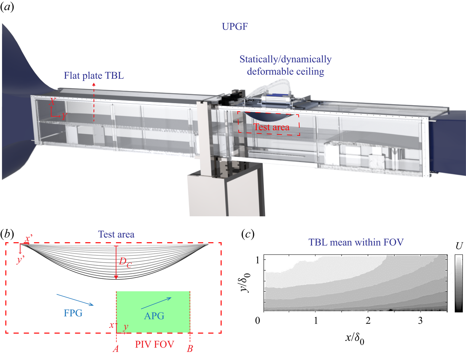
Figure 1. Illustration of the experimental details. (a) The UPGF at UIUC. The red box bounds the test area. (b) Close-up view of the test area illustrating the family of FAPGs being imposed on the flat plate. Distance  $D_c$ is the vertical distance between the flat ceiling and any deflected ceiling. The field of view (FOV) for PIV is set in the APG region and is marked by the green box. Locations $A$ and $B$ mark two key streamwise locations of interest. (c) Example TBL mean computed from PIV.
Table 1. Free-stream conditions measured at the centre of the PIV field of view for the ZPG case.
At a distance of 2.35 m from the leading edge of the flat plate, a 0.61 m section of the ceiling is replaced with the pressure gradients installation. The installation holds a flexible metal ceiling panel within the test section that is connected mechanically to an actuation mechanism located above the test section. The mechanism is used to deform the ceiling panel to the shape of an inverted convex bump of different radii, imposing FAPG sequences of different strengths. The ceiling deformation can be performed either statically or dynamically, depending on whether steady or unsteady pressure gradients are desired. The details of this set-up can be found in Parthasarathy & Saxton-Fox (Reference Parthasarathy and Saxton-Fox2022). For the present work, a series of steady pressure gradients were generated by statically deforming the ceiling to 22 different curvatures. The vertical extent of deformation ( $D_c$ in figure 1) governs the spatial strength of the pressure gradient imposed and was set to span [1–76 mm] in the current 22 cases. The maximum deflection of $D_c = 76$ mm corresponds to a minimum area ratio $(A/A_0)_{min}$ of 40 $\%$, where $A$ is the cross-sectional area above the flat plate local to a streamwise location and $A_0$ is that upstream of the test region.
The spatial distributions of the pressure coefficient,  $C_P$, created in the test area due to the 22 deformed states of the ceiling are shown in figure 2(a). The profiles were computed analytically with a steady, incompressible, one-dimensional flow assumption, using the exact geometric states of the ceiling obtained by imaging the deformed states, and were experimentally validated to be accurate within $6\,\%$ using high-frequency pressure measurements, the details of which can be found in Parthasarathy & Saxton-Fox (Reference Parthasarathy and Saxton-Fox2022). In $0< x'/L_c<0.5$, the pressure gradient is favourable, and in $0.5< x'/L_c\leq 0.82$, the pressure gradient is adverse. The flow over the ceiling was found to have separated in $x'/L_c>0.82$, rendering the pressure distributions invalid after this point. The field of view for PIV was chosen to remain within $x'/L_c \leq 0.81$. The pressure gradient variations in the test area are shown in figure 2(b,c) in terms of the acceleration parameter, $K$ (
$K$ ( $\equiv ({\nu }/{U_l^2})({{\rm d}U_l}/{{\rm d}\kern0.7pt x})$, where $U_l$ is the local average velocity outside the boundary layer), and the approximate Clauser pressure gradient parameter, $\beta _0$ ( $\equiv ({\delta ^*_0}/{\tau _{w_0}})({{\rm d}P}/{{\rm d}\kern0.7pt x}$), where $\tau _{w_0}$ is the ZPG wall shear stress estimated from $u_{\tau _0}$), valid in $0< x'/L_c\leq 0.81$. Note that since $\delta ^*_0$ and $\tau _{w_0}$ correspond to the ZPG TBL, the $\beta _0$ distributions presented are only meant to approximate the variation of the Clauser parameter in the test area.

Figure 2. (a) Coefficient of pressure distributions caused by the 22 deflected ceiling states. Darker greys correspond to higher ceiling deflection ( $D_c$). Length $L_c$ is the length of the ceiling section. Corresponding pressure gradient distributions are shown in (b) in terms of the acceleration parameter, $K$, and in (c) in terms of the approximate Clauser pressure gradient parameter, $\beta _0$, which has been computed using $u_{\tau _0}$, the ZPG friction velocity. The red dashed line in each panel indicates the location until which flow over the ceiling is attached for all test conditions and within which the PIV field of view is set.
2.2. Particle image velocimetry
The response of the flat-plate TBL to the pressure gradients imposed by the UPGF were captured using planar (two-dimensional) PIV in a  $150~{\rm mm} \times 93.75$ mm ( $L_x \times L_y$, $3.57\delta _0 \times 2.23\delta _0$) streamwise–wall-normal plane set in the APG region starting at $x' = 0.228$ or $x'/L_c = 0.5$. This field of view is indicated by the green box in figure 1. A mineral-oil-based seeding was introduced at the tunnel inlet and a Terra PIV 527-80-M dual-pulse laser was used along with a set of sheet-forming optics to illuminate the field of view. A Phantom VEO 710L camera was used to capture the particle image pairs in a frame straddling mode. Both non-time-resolved and time-resolved PIV data are collected for each of the 22 FAPG impositions. The latter has only been used in the present work for the spectral analysis presented in § 3.4. A total of 10 000 image pairs were acquired at a rate of $0.2$ kHz in the non-time-resolved dataset and 6170 image pairs at a rate of $3.755$ kHz were acquired in the time-resolved dataset. The vector fields were processed using DaVis $10.1$ software using a multi-pass approach with a final interrogation window size of $16 \times 16$. The resulting vector fields had a spatial resolution of $\Delta l^+ = 8.9$. The time-resolved fields additionally had a temporal resolution of $\Delta t^+ = 1.78$. The kinematic viscosity, $\nu$, and the friction velocity, $u_{\tau _0}$, were used in defining the viscous scales. A comparison of the measured ZPG mean and streamwise root-mean-square (RMS) velocity with direct numerical simulation of Schlatter et al. (Reference Schlatter, Örlü, Li, Brethouwer, Fransson, Johansson, Alfredsson and Henningson2009) is shown in figure 3.

Figure 3. Comparison of experimental data with benchmark direct numerical simulation (DNS) data (Schlatter et al. Reference Schlatter, Örlü, Li, Brethouwer, Fransson, Johansson, Alfredsson and Henningson2009): (a) streamwise velocity; (b) streamwise RMS velocity.
2.3. Strength of pressure gradients within the PIV field of view
Under the different deflections of the ceiling panel, the TBL within the PIV field of view locally experiences a spatially strengthening APG. For higher ceiling deflections, the local APG is stronger, and so is the upstream FPG as seen in figure 2. While the local magnitudes of the non-dimensional parameters ( $K$ and $\beta _0$ in $0.5 \leq x'/L_c \leq 0.81$ in figure 2b,c) capture the local APG strengths, they do not signify the presence or strengths of the upstream FPGs that strongly affect the APG TBL response. It is an open question as to what cumulative parameters are most important for spatially varying pressure gradients. A few candidate parameters that may influence the total response of the system are reported in table 2, some of which are inspired by Vinuesa et al. (Reference Vinuesa, Örlü, Sanmiguel Vila, Ianiro, Discetti and Schlatter2017).
Table 2. Variables representing the strength of the pressure gradients imposed by each ceiling deflection. Definitions are provided in the text.

The pressure gradient cases are numbered 1 through 22 in order of increasing FAPG strength (or increasing ceiling deflection). Parameters  $K_{max}$ and $\beta _{max}$ are the maximum $K$ and $\beta$, respectively, realised within the test area in each case. Parameters $\overline {K(x)_B}$ and $\overline {\beta (x)_B}$ are the spatially averaged $K$ and $\beta$, respectively, computed as $\overline {Q(x)_B} \equiv ({1}/{(x_B - x_0)})\int _{x_0}^{x_B} Q \,{{\rm d}\kern0.7pt x}$, where $x_0$ corresponds to $x'/L_c = 0$, the beginning of the FPG region, and $x_B$ corresponds to $x/L_x = 1$, the last station of the PIV field of view. Here $Q$ is either $K$ or $\beta$. Note that although the integrated $\overline {K(x)_B}$ takes positive values for all cases, the imposed conditions are not equivalent to purely FPGs with matched $\overline {K(x)}$. This is discussed in § 3.1, further emphasising the need to explore parameters that sufficiently represent history effects for sequential pressure gradients. The rapid spatial changes in the pressure gradients imposed emerged as important to the TBL response, prompting the definition of the maximum ${\rm d}K/{{\rm d}\kern0.7pt x}$ in each case, reported in the table. Since an appropriate variable is an open question, the overall pressure gradient strengths imposed in the different cases will be referred to by $\overline {K(x)_B}$ in most of the discussion. Parameter $\overline {K(x)_B} \times 10^6$ is denoted by $\bar {K}$ for convenience.
3. Results and discussion
3.1. Statistics
The mean and Reynolds stresses of the TBL under the imposed pressure gradients are presented and discussed for 6 cases out of the 22 sets. Statistics for all the cases are included in the supplementary material available at https://doi.org/10.1017/jfm.2023.429. The six cases presented here correspond to sets [1, 5, 9, 13, 17, 22] in table 2, with  $\bar {K} = [0 0.25\ 0.5\ 0.74\ 0.96\ 1.2]$. The streamwise mean velocity, streamwise Reynolds stress (u-RS), wall-normal Reynolds stress (v-RS) and Reynolds shear stress (uv-RS) are shown in figure 4. The statistics are scaled with local outer units (edge velocity $U_e$ and boundary layer thickness $\delta$) obtained using the diagnostic plot technique for pressure gradient TBLs (Vinuesa et al. Reference Vinuesa, Bobke, Örlü and Schlatter2016). Parameters $U_e$ and $\delta$ naturally vary in $x$ and with $\bar {K}$ as the boundary layer accelerates and decelerates. Scaling using these variables affects the statistical trends to be discussed, but the overall trends remain the same regardless of local or global scaling. This is demonstrated in the Appendix. Uncertainties in the statistics were computed with 95 $\%$ confidence, following Benedict & Gould (Reference Benedict and Gould1996), at two spatial locations ( $x/L_x = 0$ and $x/L_x = 1$) and averaged. The uncertainties were then averaged along the wall-normal direction and are as follows, in the format ‘average [minimum, maximum]’: in the streamwise mean, 0.21 $\%$ [0.08 $\%$, 0.82 $\%$]; in the u-RS, 3.06 $\%$ [2.22 $\%$, 3.63 $\%$]; in the v-RS, 3.38 $\%$ [2.86 $\%$, 4.14 $\%$]; in the uv-RS, 3.46 $\%$ [2.47 $\%$, 10.18 $\%$]. The streamwise locations from which the data shown in figure 4 are extracted are indicated above each panel in terms of $x/L_x$; $x = 0$ at the upstream end of the PIV field of view (station A) and $x = L_x$ at the downstream end (station B).

Figure 4. Statistics as a function of space ( $x$) and pressure gradient ( $\bar {K}$). (a) Mean streamwise velocity. (b) Streamwise Reynolds stress. (c) Wall-normal Reynolds stress. (d) Reynolds shear stress. The streamwise location from which the statistics are extracted is indicated above each panel in red in terms of $x/L_x$. Stronger pressure gradients or higher $\bar {K}$ are marked using darker greys. Here $\bar {K} = 0$, 0.25, 0.5, 0.74, 0.96 and 1.2 for the cases shown.
The mean velocity profiles show evidence of upstream acceleration from the FPG region and local deceleration from that accelerated state throughout the APG region. At  $x/L_x = 0$, at the transition from FPG to APG, the mean velocity profiles shown in figure 4(a) are seen to become fuller as the overall pressure gradient strength is increased ( $\bar {K}$, darker data points), which is an effect of stronger acceleration caused by stronger upstream FPGs for higher $\bar {K}$. The mean velocities at this station resemble profiles extracted from successive spatial stations in a region of FPG (Ichimiya et al. Reference Ichimiya, Nakamura and Yamashita1998). At all locations except $x/L_x = 0$, the shown data are in a local APG. Moving along $x/L_x$ at a given $\bar {K}$, the mean velocity gradient in $y < 0.2\delta$ decreases due to the deceleration caused by the APG. For a given location within $x/L_x > 0$, the mean profiles become fuller with increasing $\bar {K}$, despite higher $\bar {K}$ corresponding to a stronger local APG in $x/L_x > 0$. This is because for higher $\bar {K}$, the upstream FPG in the region $x/L_x < 0$ is also stronger, creating a more accelerated incoming TBL on which the APG locally acts. Comparing $x/L_x = 0$ and $x/L_x = 1$, the mean velocity profiles are observed to decelerate through the APG region, but to remain more accelerated than the equivalent ZPG case. This could be expected from the $C_P$ distributions of figure 2(a), where $C_P$ remains negative through the APG region, much like the suction side of typical airfoils at moderate angles of attack, where the strong upstream FPG causes the APG flow to remain faster than the incoming flow despite the local deceleration. Mean velocity variations under other FAPG sequences also exhibit similar trends in the mean, such as in the flow over a bump in Cavar & Meyer (Reference Cavar and Meyer2011).
The Reynolds stresses (figure 4b–d) show two main trends. First, suppression and the appearance of a bimodal structure coming out of the spatially varying FPG; and, second, the strengthening of the near-wall peak across the APG region. Both behaviours show traits specific to the spatially varying pressure gradient used in this experiment. The u-RS at the transition from FPG to APG,  $x/L_x = 0$, in figure 4(b) exhibits a suppression of the stress throughout the measured boundary layer with increasing $\bar {K}$, as is expected of an accelerated TBL (Volino Reference Volino2020). However, a two-peak structure appears, with the two peaks separated by a ‘knee point’ at their valley. At $x/L_x=0$, the knee point can be quantified as a local minimum for the three largest pressure gradients shown ( $\bar {K} \geq 0.74$). For these pressure gradients, the wall-normal location of the knee point reduces with increasing pressure gradient, forming at $y = 0.35 \delta$ when $\bar {K} = 0.74$ and at $y = 0.24 \delta$ when $\bar {K} = 1.2$. At the same streamwise location, $x/L_x = 0$, v-RS and uv-RS shown in figures 4(c) and 4(d), respectively, also show a suppression of stresses caused by the upstream FPG for increasing $\bar {K}$ and the formation of a two-peak structure. For large pressure gradients, $\bar {K} \geq 0.96$, the magnitude of the second peak exceeds that of the first peak. The wall-normal location of the local minimum approximately coincides with that formed in the u-RS (figure 4b). The wall-normal location of the first peak in v-RS and uv-RS at $x/L_x = 0$ shifts away from the wall as $\bar {K}$ increases, from $y = 0.097 \delta$ at $\bar {K}=0$ to $y = 0.136 \delta$ at $\bar {K}=1.2$.
Along the streamwise direction, for a given  $\bar {K}$, the knee point generally persists, and its wall-normal location moves away from the wall. The knee point in the uv-RS is located at $y = 0.36 \delta$ for $\bar {K} = 1.2$ and $x/L_x=1$, versus $y=0.24\delta$ at $x/L_x=0$. In $x/L_x > 0$, the peak moves closer to the wall and reverts back to $y = 0.1 \delta$ at $x/L_x = 1$ for all $\bar {K}$. Below the knee point location, all the stresses are seen to increase with streamwise distance in the APG region, while above the knee point, the stresses are seen to decrease. In the u-RS shown in figure 4(b), this increase and decrease in magnitude below and above the knee point, respectively, cause the knee point to become indistinguishable for $x/L_x \geq 0.8$. In the v-RS and uv-RS shown in figure 4(c,d), the increase in magnitude below the knee point with increasing $x/L_x$ yields a dramatic increase in the magnitude of the first peak (by factors of 2.8 and 4.4, respectively, for $\bar {K} = 1.2$). For $x/L_x > 0$, the Reynolds stresses in figure 4(b–d) are weaker for larger $x/L_x$ or higher $\bar {K}$ over most of the boundary layer, despite larger $x/L_x$ indicating longer exposure to an APG and higher $\bar {K}$ corresponding to a stronger local APG imposition. For example, at $x/L_x = 1$, the u-RS magnitude in the wake region at $y = 0.4 \delta$ is 43 $\%$ lower at $\bar {K} = 1.2$ compared with that at $\bar {K} = 0$.
Overall, there are two key observations from the Reynolds stresses. The first is that the Reynolds stresses of the current APG TBL exhibit knee points and multiple peaks. As introduced in § 1, inflectional footprints in second-order statistics indicate the presence of an internal layer within the TBL. A discontinuity in surface curvature (Matai Reference Matai2018), a step change in surface roughness (Hanson & Ganapathisubramani Reference Hanson and Ganapathisubramani2016), a change in the sign of pressure gradient encountered (Tsuji & Morikawa Reference Tsuji and Morikawa1976), the application of blowing/suction (Simpson Reference Simpson1971) can all trigger the formation of internal layers, which have been shown to dominate the near-wall dynamics of the TBL, especially through skin friction. Thus, an internal layer is inferred to have formed in the present experiments due to the rapid changes in pressure gradients imposed, giving rise to the inflectional stress profiles. The second observation is that the trends with which the magnitude of Reynolds stresses vary with increasing local APG strength along  $x$ and $\bar {K}$ are different from (in fact, opposite to) well-established APG effects. The trends in $x$ showing a strengthening inner peak and weakening/frozen outer peak are consistent with the APG statistics of bump/hill TBLs with internal layers. The growth of the inner peak is attributed to the presence and growth of this layer (Cavar & Meyer Reference Cavar and Meyer2011; Matai & Durbin Reference Matai and Durbin2019), yet much is unknown about the nature of turbulence within these internal layers. The weakening/frozen outer peak has previously been suggested to be effects of convex curvature (Baskaran et al. Reference Baskaran, Smits and Joubert1987; Balin & Jansen Reference Balin and Jansen2021), but similar trends observed in the current experiments where the measurements have been made on the flat wall indicate that surface curvature may not explain this peculiar behaviour. These aspects are investigated in the reminder of this paper. The decreasing Reynolds stresses throughout most of the boundary layer with increasing $\bar {K}$ is likely a direct result of the stronger upstream FPG for cases with higher $\bar {K}$, as suggested by the lasting influence of the upstream FPG on the turbulent mean throughout the recorded APG region. This significant history effect is also studied in parallel in the subsequent sections.
3.2. Internal layers
The presence and growth of internal layers, whose signatures were seen to dominate the statistics, are investigated in this section with the goals of identifying the pressure gradient strengths for which an internal layer is clearly present, characterising the internal layer's spatial growth and characterising the nature of turbulence within and outside this layer.
To correctly bifurcate the boundary layer as regions within and outside the internal layer, the edge of the internal layer needs to be detected. Several techniques to approximate the edge have been introduced by the community studying step changes in surface roughness. These methods are summarised in Rouhi, Chung & Hutchins (Reference Rouhi, Chung and Hutchins2019). A simple half-power plotting scheme proposed by Antonia & Luxton (Reference Antonia and Luxton1971) has been adopted in this study. In this scheme, mean velocities are plotted with respect to  $y^{1/2}$. When an internal layer is present, two regions with differing linear trends appear separated by a ‘kink’. The intersection point between linear fits of these two regions is said to approximately correspond to the wall-normal height of the internal layer. Antonia & Luxton (Reference Antonia and Luxton1971) supported this convenient scaling using dimensional arguments and the method has been widely used since (Jacobi & McKeon Reference Jacobi and McKeon2011; Hanson & Ganapathisubramani Reference Hanson and Ganapathisubramani2016; Li et al. Reference Li, de Silva, Chung, Pullin, Marusic and Hutchins2022), including in a study of internal layers past a step roughness change under APGs (Schofield Reference Schofield1975) and a study on internal layers in sequences of curvatures and pressure gradients (Bandyopadhyay & Ahmed Reference Bandyopadhyay and Ahmed1993). Half-power plots of the mean velocity profiles at stations $A$ and $B$ are shown for all 22 pressure gradient cases in figures 5(a) and 5(b), respectively. The profiles have been extracted from the wall-normal region relevant to the internal layer identification, $0.07 < y/\delta _0 < 0.29$, and the wall-normal coordinate has been non-dimensionalised by the ZPG boundary layer thickness. Darker profiles mark stronger FAPGs (or higher $\bar {K}$). At both stations, the ZPG case does not exhibit a change in slope. The pressure gradient case for which a kink appears is not obvious by visual inspection.

Figure 5. Detection of internal layer edge. Half-power plot of the mean velocity profiles in  $0.07 < y/\delta _0 < 0.29$ at (a) station $A$ and (b) station $B$. (c) Half-power plot of the mean velocity profile at station $B$ for $\bar {K} = 1.2$. The red circle marks the kink identified programmatically by finding the maximum slope difference, $\Delta _p$, between linear fits of the data when partitioned at different points ( $y_p$). Blue dashed line marks the data point corresponding to the wall-normal height of the internal layer obtained. (d) Difference $\Delta _p$ for the same case and location as (c). Velocity $U_0$ is the constant free-stream velocity. (e) Edge of the internal layer for $\bar {K} = 1.2$ (black line) overlaid on the average spanwise vorticity field.
To systematically identify the kink, an algorithm is implemented that partitions the half-power plot data at different points (starting from the third data point) and linearly fits the data below and above the partitioning point. The difference between the slopes of the linear fits is found. The difference is the highest when the data are partitioned at the kink. The intersection between the linear fits with the kink as the partitioning point is the location of internal layer edge. This process is illustrated in figure 5(c,d) for  $\bar {K} = 1.2$ at station $B$. The latter figure shows the slope differences ( $\Delta _p$) between the linear fits as the partitioning point ( $y_p$) is varied. Difference $\Delta _p$ is computed as
 \begin{equation} \Delta_p(y_p) =\left[ \frac{U(y_p) - U(y_i)}{\sqrt{y_p - y_i}} - \frac{U(y_f) - U(y_p)}{\sqrt{y_f - y_p}} \right] \frac{\sqrt{\delta_0}}{U_0}, \end{equation}
and is plotted as a function of the half-power of  $y_p$ in figure 5(d). Here $y_i = 0.07\delta _0$ and $y_f = 0.29\delta _0$. The partitioning point that corresponds to the maximum slope difference $\Delta _p$ is the programmatically obtained kink and is marked with a red circle in figure 5(c,d). Linear fits of the data below and above the kink intersect at the local edge of the internal layer, marked with the blue dashed line in figure 5(c). The detected wall-normal heights of the internal layer at successive streamwise locations for $\bar {K} = 1.2$ are shown in figure 5(e) as a black line overlaid on the average spanwise vorticity field. The internal layer is seen to spatially grow, as expected, and can be observed to be a region of significant shear, outside which the average spanwise vorticity is considerably less.
Using this edge detection method on pressure gradient cases 1 through 7 resulted in the maximum slope difference ( ${\Delta _p}$) being less than 0.2 and did not result in a consistent detection of kinks (i.e. subsequent kinks were not spatially well correlated), suggesting that an internal layer is only clearly present in cases 8 through 22 for which $\bar {K} \geq 0.45$ or $-({\rm d}K/{{\rm d}\kern0.7pt x})_m \delta _0 \geq 0.49 \times 10^{-6}$. For these cases, the edge of the internal layer exhibited power-law growth within the APG region as $\delta _i \propto x^{\alpha }$. The growth rates were computed and are shown in figure 6 as a function of $\bar {K}$. The growth rate is seen to increase with increase in strength of the FAPG and the relationship appears to be linear. The linear relationship was found to be true even when $\alpha$ was plotted against other pressure gradient parameters listed in table 2. Additionally, for all cases shown, the growth rate is greater than 1. In contrast, the growth rates reported for internal layers in TBLs past step changes in roughness have consistently been less than 1: $0.4 < \alpha < 0.8$ for smooth to rough flows and $0.2 < \alpha < 0.4$ for rough to smooth flows. This difference is likely due to the growth of the current internal layers in a local APG and is consistent with the growth rates deduced from previous studies of pressure gradient sequences where the approximate edge of the internal layer has been reported at discrete spatial locations (Tsuji & Morikawa Reference Tsuji and Morikawa1976; Baskaran et al. Reference Baskaran, Smits and Joubert1987; Uzun & Malik Reference Uzun and Malik2022).

Figure 6. Spatial growth rates of the internal layer within the APG region for cases where a clear internal layer is deemed to be present,  $\bar {K} \geq 0.45$.
As demonstrated by figure 5(e) for the strongest FAPG case, the internal layer is a region of strong spanwise vorticity. However, average vorticity magnitudes are not good indicators of whether the region contains significant swirling motion or is a region of pure shear. To elucidate this and to characterise the internal layer further for the different FAPG strengths imposed, a vortex identification technique is used. The swirling strength criterion (or  $\lambda _{ci}$ method) is chosen as it is frame-independent and can distinguish between rotation and shear (Adrian, Christensen & Liu Reference Adrian, Christensen and Liu2000). The spanwise swirling strength, $\lambda _{ci}$, is obtained from the two-dimensional velocity gradient tensor. Swirling strength $\lambda _{ci} > 0$ indicates the presence of a vortex. Defining $\varLambda _{ci} \equiv \lambda _{ci} \times {\omega }/{|\omega |}$ assigns the direction of instantaneous vorticity to the swirling strength.
The RMS of the swirling strength parameter,  $\varLambda ^{RMS}_{ci}$, characterises the strength of vortices at a given location (Wu & Christensen Reference Wu and Christensen2006). The wall-normal variation of $\varLambda ^{RMS}_{ci}$ is studied to understand the composition of swirling motion within the internal layer. Figure 7(a) shows the wall-normal profiles of $\varLambda ^{RMS}_{ci}$ for the ZPG case ( $\bar {K} = 0$) and the strongest FAPG case ( $\bar {K} = 1.2$) at different streamwise locations. Local outer scaling has been used in the non-dimensionalisation, as in the case of the statistics. The analysis is restricted to $y \geq 0.1 \delta$ since the derivatives computed (in computing the velocity gradient) are noisy closer to the wall. The ZPG $\varLambda ^{RMS}_{ci}$ (marked in black in figure 7a) shows the presence of strong vortices near the wall and the strength gradually decreases away from the wall, consistent with Lee et al. (Reference Lee, Lee, Lee and Sung2010). The profiles for the strongest FAPG case are shown at station $A$ (
$A$ ( $x/L_x = 0$, red), at station $B$ (
$B$ ( $x/L_x = 1$, blue) and at the middle of these two locations ( $x/L_x = 0.5$, green). At station $A$, where the TBL has experienced a strong upstream FPG and encounters the pressure gradient sign change, a significant decay in vortex strength is seen throughout the boundary layer compared with the ZPG profile. While a peak in the ZPG case is expected to have formed much closer to the wall (not resolved here, but see Lee et al. (Reference Lee, Lee, Lee and Sung2010)), a peak is observed in the FAPG case at station $A$ at $y = 0.14 \delta$. For milder pressure gradients (not shown), the peak was found to be narrower and formed closer to the wall for the same streamwise location, for example, at $y = 0.097\delta$ for $\bar {K} = 0.45$. At $x/L_x = 0.5$ (figure 7a, green), the peak is seen to have grown and to have shifted closer to the wall. In $y \geq 0.26\delta$, the locally scaled strength of vortices has remained the same as at station $A$ (
$A$ ( $0.73\delta \leq y \leq \delta$) or decreased further ( $0.26\delta \leq y \leq 0.73\delta$). At this streamwise location, the boundary layer has experienced a locally APG region for 2.5 average boundary layer thicknesses. From $x/L_x = 0.5$ to $x/L_x = 1$, in keeping with the trend, the peak is seen to grow significantly and to move closer to the wall while also broadening in the wall-normal direction. Outside this broad peak ( $y \geq 0.35\delta$), the vortex strength is observed to have increased compared with $x/L_x = 0.5$ (while remaining considerably less than the increase in $y \leq 0.35\delta$) and to stay approximately constant across this wall-normal region.

Figure 7. (a) Outer-scaled RMS of swirling strength parameter ( $\varLambda _{ci}$) with respect to wall-normal height for select FAPG cases and streamwise locations indicated by the legend. The increase in $\varLambda _{ci}$ in $y/\delta < 0.4$ for $\bar {K} = 1.2$ suggests the internal layer to be a growing region of strong vortex activity. (b) Plots of $\varLambda ^{RMS}_{ci}$ at $y/\delta = 0.1$ for all FAPG cases investigated, at stations $A$ (
$A$ ( $x/L_x = 0$) and $B$ (
$B$ ( $x/L_x = 0$). In $\bar {K} \geq 0.45$, identified earlier as the pressure gradients for which an internal layer is clearly present, a significant increase $\varLambda ^{RMS}_{ci}$ is observed from stations $A$ to $B$.
$B$.
The structure of  $\varLambda ^{RMS}_{ci}$ in the APG region of this experiment is different from that of APG TBLs originating from a ZPG region, where a dramatic increase in $\varLambda ^{RMS}_{ci}$ is expected to be centred in the wake region. For example, Lee et al. (Reference Lee, Lee, Lee and Sung2010) saw an increase of up to 3.5 times the ZPG value at $y = 0.5\delta$ for a mild APG with $\beta = 1.68$. The weakening of vortices observed at station $A$ in figure 7(a) can be expected as a result of the stabilising influence of the upstream FPG. But the presence of the peak at $y = 0.14\delta$ is not an expected FPG effect and is associated with the presence of the internal layer. The internal layer, then, appears to be a region of increased swirling motion compared with the rest of the boundary layer. The wall-normal location of the scaled $\varLambda ^{RMS}_{ci}$ peak was observed to remain within the internal layer, while the peak magnitude grew significantly with $x$. In the outer layer, only a weak increase in scaled $\varLambda ^{RMS}_{ci}$ was observed from stations $A$ to $B$, while the unscaled $\varLambda ^{RMS}_{ci}$ was found to remain unchanged under the local APG.
The effect of the imposed FAPG magnitude on the strength of vortices close to the wall is quantitatively studied by tracking scaled  $\varLambda ^{RMS}_{ci}$ at $y = 0.1\delta$ for each case. This is shown in figure 7(b) at stations $A$ (red markers) and $B$ (blue markers). Strength parameter $\varLambda ^{RMS}_{ci}$ at $y = 0.1\delta$ was chosen to be tracked rather than the magnitude of the peak observed in figure 7(a) to enable plotting for milder pressure gradient cases for which no peak was found/resolved. At station $A$, figure 7(b) shows that the outer-scaled $\varLambda ^{RMS}_{ci}$ at $y = 0.1\delta$ reduces as $\bar {K}$ increases, as expected. The rate of reduction, however, is considerably milder in $\bar {K} < 0.45$ and stronger in $\bar {K} \geq 0.45$. Similarly at station $B$, the variations with $\bar {K}$ are slightly different for $\bar {K} < 0.45$ and $\bar {K} \geq 0.45$, remaining almost constant in the former range and increasing slowly in the latter. Larger differences were observed above and below $\bar {K} = 0.45$ in the unscaled $\varLambda ^{RMS}_{ci}$, although not shown here. For a given $\bar {K}>0$, the strength of vortices at $y = 0.1\delta$ is seen in figure 7(b) to increase from stations $A$ to $B$. For $\bar {K} = 0.45$, a 19 $\%$ increase is observed, and for $\bar {K} = 1.2$, a $283\,\%$ increase is observed. As mentioned earlier, this increase in $\varLambda ^{RMS}_{ci}$ near the wall with $x$ is associated with the growth of the internal layer, which appears to contain increasingly strong swirling motions within it as it grows in the APG region. In stronger FAPG cases, the rapid spatial pressure gradient changes are more severe, resulting in a stronger and faster-growing internal layer (figure 6) that causes a more dramatic strengthening of swirling motion near the wall. Qualitatively similar trends resulted when $\varLambda ^{RMS}_{ci}$ was averaged over different regions in $y = [0.1\delta, 0.3\delta ]$ as well, instead of being tracked at $y=0.1\delta$ as done in figure 7(b).
Although the streamwise and wall-normal variations in  $\varLambda ^{RMS}_{ci}$ for the different pressure gradients imposed indicate that vortices within the internal layer strengthen, it does not reveal if this layer is composed of an increased number of vortices or if it has caused the swirling strengths of existing vortices to increase. Hence, vortices in the flow are detected and counted across all ensembles. The universal threshold given by $|{\varLambda _{ci}}/{\varLambda ^{RMS}_{ci}} | \geq 1.5$ is used to detect vortices in $3 \times 3$ windows of the data in the streamwise and wall-normal directions. The resulting window size is $0.033\delta _0 \times 0.033\delta _0$. A vortex satisfying the threshold is counted only if it occupies at least a $2 \times 2$ window, consistent with standard practices in the literature used while estimating vortex population densities (Wu & Christensen Reference Wu and Christensen2006). A large vortex occupying multiple 3 $\times$ 3 windows is appropriately counted as 1. Prograde and retrograde vortices are counted separately. Figure 8(a) shows the number ( $N_V$) of prograde (solid lines) and retrograde (dashed lines) vortices detected across the ensembles as a function of the wall-normal height for the ZPG case ( $\bar {K} = 0$, black), and for the strongest FAPG ( $\bar {K} = 1.2$) at stations $A$ (
$A$ ( $x/L_x = 0$, red) and $B$ (
$B$ ( $x/L_x = 1$, blue). Similar to figure 7(b), figure 8(b) shows $N_V$ at $y= 0.1\delta$ plotted as a function of the overall pressure gradient strength for stations $A$ and $B$.
$B$.

Figure 8. (a) Number of vortices detected as a function of wall-normal height for the ZPG case ( $K=0$) and the strongest FAPG case ( $K = 1.2$) at stations $A$ (
$A$ ( $x/L_x = 0$) and $B$ (
$B$ ( $x/L_x = 1$). Solid lines represent prograde vortices and dashed lines represent retrograde vortices. An increase in the number of total number of vortices occurs in $y/\delta < 0.3$ for $K = 1.2$, a wall-normal region within the internal layer identified. (b) Plots of $N_V$ at $y/\delta = 0.1$ for all FAPG cases investigated at stations $A$ (
$A$ ( $x/L_x = 0$) and $B$ (
$B$ ( $x/L_x = 1$). Squares mark prograde and circles mark retrograde vortices. In $\bar {K} \geq 0.45$, identified earlier as the pressure gradients for which an internal layer is clearly present, a significant increase the total number of vortices from stations $A$ to $B$ can be deduced.
For  $\bar {K} = 0$, the wall-normal variations in figure 8(a) show that the number of prograde vortices in the ZPG TBL is 1.4 to 5.8 times more than the number of retrograde vortices. The prograde vortices are largest in population near the wall and drop off with increase in height from the wall, while the retrograde vortices show a maximum near the outer edge of the logarithmic region. These variations are consistent with literature observations of vortex populations in ZPG TBLs (Lee et al. Reference Lee, Lee, Lee and Sung2010; Herpin et al. Reference Herpin, Stanislas, Foucaut and Coudert2013). Under the strongest FAPG imposed ( $\bar {K} = 1.2$), at station $A$, the population of both prograde and retrograde vortices throughout the boundary layer is seen to have reduced as a result of the upstream FPG. The retrograde vortices have reduced in population everywhere, while the prograde vortices show a manner of reduction similar to the scaled $\varLambda ^{RMS}_{ci}$ shown in figure 7(a), exhibiting a peak at a similar wall-normal height embedded within the internal layer. Note that because of the windowing involved with the vortex identification, the wall-normal resolution is lower in figure 8(a) than in figure 7(a). From stations $A$ to $B$, the number of prograde vortices near the wall increases significantly as the internal layer grows in the local APG, and the peak moves closer to the wall, again qualitatively similar to the variation in figure 7(a). Outside the broad peak at station $B$ (in $y > 0.3 \delta$), the number of vortices at a given wall-normal location slightly decreases compared with that at station $A$. This is despite the TBL experiencing a strengthening APG over 5 average boundary layer thicknesses by the time it reaches station $B$, which may have been expected to cause an increase in the population of vortices. The retrograde vortices, on the other hand, show a different variation. Their number decreases within the internal layer in $0.12\delta < y < 0.31\delta$ and stays constant outside the layer.
All the population trends discussed here for  $\bar {K} = 1.2$ were found to be consistent across cases with $\bar {K} \geq 0.45$. The variation from stations $A$ to $B$ at $y = 0.1\delta$ is tracked for all FAPG cases imposed and shown in figure 8(b). The figure reveals the strong increase in the number of prograde vortices as a result of the internal layer growth for $\bar {K} \geq 0.45$. In $\bar {K} < 0.45$, only a weak change is observed. This reinforces the identification of $\bar {K} = 0.45$ as the average pressure gradient for which an internal layer is clearly present and is strong enough to modify the TBL response significantly. The number of retrograde vortices at $y = 0.1\delta$ changes less in $x$ than prograde, but a mild trend of increasing vortices can be deduced for the strong FAPGs with $\bar {K}>0.8$.
While the interpretations of prograde and retrograde vortices in terms of the structure of the TBL are still debated, they have often been associated with hairpin vortices (Natrajan, Wu & Christensen Reference Natrajan, Wu and Christensen2007; Gao, Ortiz-Duenas & Longmire Reference Gao, Ortiz-Duenas and Longmire2011; Herpin et al. Reference Herpin, Stanislas, Foucaut and Coudert2013). Prograde vortices are considered signatures of the heads of hairpin vortices and retrograde, of the necks. Isolated retrograde vortices have also been said to form when hairpin vortices merge in the spanwise direction (Tomkins & Adrian Reference Tomkins and Adrian2003). The current analysis suggests that the internal layer is composed of an increased number of hairpin vortices, whose heads populate  $0.1\delta \leq y \leq 0.3$ and necks and tails extend down below $y = 0.1\delta$. The latter could explain the reduced population of retrograde vortices within most of the internal layer. Another likely explanation is that the retrograde vortices are less successful in resisting the increased mean shear due to the internal layer, which opposes their rotation. Overall, when the internal layer is present, the flow clearly exhibits an increased total number of vortices within that region compared to the rest of the boundary layer (as seen in figure 8a), which further increases as the flow progresses through the APG region and the internal layer grows. This increased population is at least partially responsible for the increased vortex strength seen in figure 7. In contrast, in a TBL that only experiences an APG, the APG causes an increase in the population of prograde vortices centred in the wake region and no significant change in the population of retrograde vortices at all wall-normal locations (Lee et al. Reference Lee, Lee, Lee and Sung2010).
3.3. Turbulent production
It has been established that the FAPG conditions imposed in the current experiments have a strong influence on the TBL response, including a lasting effect of the upstream FPG on the downstream APG region, the formation of an internal boundary layer in cases where  $\bar {K} \geq 0.45$ and subsequent changes to the statistics and vortex organisation of the TBL. With a better understanding of the internal layer and its characteristics, the reasons for the trends in the statistics observed in § 3.1 with $x$ and $\bar {K}$ are revisited by investigating the production rates of turbulent kinetic energy (TKE) ( $P_k$) and Reynolds shear stress ( $P_{uv}$). These quantities are computed as
 \begin{equation}
\left.\begin{gathered}
P_k ={-} \overline{u'_i u'_j} \frac{\partial
\bar{u}_i}{\partial x_j}, \\ P_{uv} ={-} \left(
\overline{u'_1 u'_i} \frac{\partial \bar{u}_2}{\partial x_i}
+ \overline{u'_2 u'_i} \frac{\partial \bar{u}_1}{\partial
x_i} \right), \end{gathered}\right\}
\end{equation}
\begin{equation}
\left.\begin{gathered}
P_k ={-} \overline{u'_i u'_j} \frac{\partial
\bar{u}_i}{\partial x_j}, \\ P_{uv} ={-} \left(
\overline{u'_1 u'_i} \frac{\partial \bar{u}_2}{\partial x_i}
+ \overline{u'_2 u'_i} \frac{\partial \bar{u}_1}{\partial
x_i} \right), \end{gathered}\right\}
\end{equation}
where  ${u_i}$ are instantaneous velocities, overbar denotes ensemble average, primed quantities are fluctuations about the mean and subscripts 1 and 2 denote component along the streamwise and wall-normal directions, respectively. Here $i$ and $j$ each take values ${1,2}$. Before computing the derivatives, the data in the $[313 \times 197]$ grid were interpolated into a grid of $[1000 \times 1000]$ using a shape-preserving interpolant: piecewise cubic Hermite interpolating polynomial. The derivatives were then computed using second-order central difference everywhere except at the edges where single-sided difference was used.
Outer-scaled wall-normal profiles of  $P_k$ and $P_{uv}$ are shown in figure 9 at stations $A$ and $B$ for the six FAPG cases focused on in § 3.1 and at six streamwise stations for the strongest FAPG case to show a representative streamwise evolution. Stronger pressure gradients and successive streamwise stations are marked by darker greys in the figure. At station $A$, the production rates of TKE and uv-RS in the ZPG case ( $\bar {K} = 0$, lightest grey in figure 9a,c) follow an expected variation in the wall-normal direction with maximum $P_k$ and $P_{uv}$ occurring closer to the wall, which gradually decay to 0 at the edge of the boundary layer. The same qualitative variation is exhibited by the mild FAPG case with $\bar {K} = 0.25$ at station $A$, along with a slight reduction in the magnitudes of production observed throughout the boundary layer due to upstream FPG. For $\bar {K} \geq 0.5$, the production of TKE and uv-RS at this station decrease considerably, as expected, under the stabilising action of the strengthening upstream FPG. But the wall-normal structure assumed by the production profiles is different for $\bar {K} \geq 0.5$. Production rate $P_k$ shows a larger difference between the rates of reduction within and outside of $y \sim 0.2\delta$ compared with $\bar {K} < 0.5$, suggesting the appearance of a production peak within the internal layer, although the peak itself has not been resolved. Above $y \sim 0.2\delta$, $P_k$ almost decreases to 0, consistent with the observation by Balin (Reference Balin2020) that the TKE production is ‘turned off’ in the outer layer at the exit of the FPG region of a bump flow. Parameter $P_{uv}$ shows the formation of a peak in $y \sim 0.2\delta$ that moves away from the wall for higher $\bar {K}$, outside of which the shear stress production is significantly lower (but not negligible).

Figure 9. Production of TKE at stations (a)  $A$ and (b) $B$ for $\bar {K} = 0$, 0.25, 0.5, 0.74, 0.96 and 1.2. Stronger FAPGs (or higher $\bar {K}$) are marked by darker greys. Production of Reynolds shear stress at stations (c) $A$ and (d) $B$ for the same FAPG cases as (a,b). (e) Production of TKE for $\bar {K} = 1.2$ at streamwise stations $x/L_x = 0$, 0.2, 0.4, 0.6, 0.8 and 1. Successive streamwise stations are marked by darker greys. (f) Production of Reynolds shear stress for $\bar {K} = 1.2$ at the same streamwise stations as (e).
As the boundary layer moves through a local APG region to reach station  $B$, the changes to the production in TKE and uv-RS are shown at successive streamwise stations in figures 9(e) and 9(f), respectively, for case $\bar {K} = 1.2$, to demonstrate the streamwise variation. Within the internal layer, a strong increase in production is observed as the layer grows in $x$, resulting in an increase of over an order of magnitude in the TKE production. The wall-normal region over which the increase occurs in figure 9(e,f) widens with $x$, consistent with the wall-normal growth of the internal layer with $x$. In contrast to the production within the internal layer, the production in the outer layer is seen to remain frozen throughout the local APG region. The production of TKE and uv-RS remaining ‘turned off’ within the APG region could partially explain the reduction in outer peak magnitudes of the Reynolds stresses observed with $x$ in figure 4(b–d) for the stronger pressure gradients, in contrast to the increase expected of a typical APG TBL (Gungor et al. Reference Gungor, Maciel and Gungor2022). Lastly, the production profiles that result at station $B$ for the six FAPG cases are shown in figure 9(b,d). With increase in $\bar {K}$ imposed, the production close to the wall and within the internal layer increases and that outside decreases as a result of the stronger upstream FPG associated with higher $\bar {K}$. Comparing figure 9(a) with 9(b) and figure 9(c) with 9(d) shows the changes between stations $A$ and $B$ in $P_k$ and $P_{uv}$ for each FAPG case considered. The strongest increase in production within the internal layer happens for $\bar {K} = 1.2$, as can be expected. In the outer layer, none of the cases show any significant change in the production of TKE and uv-RS from stations $A$ to $B$.
$B$.
3.4. Energy spectra
The energy-carrying scales in the TBL are studied by computing the one-dimensional premultiplied Fourier power spectral densities (PSDs) of the streamwise and wall-normal velocity fluctuations. The objective is to assess the trends in scale composition and how they change relative to the ZPG as the pressure gradient is changed along  $x$ and $\bar {K}$. The PSDs are premultiplied by the streamwise wavenumber.
The PSDs of the streamwise velocity fluctuations are shown in figure 10 for select cases and streamwise locations. Figure 10(a) shows the ZPG spectrum. The second row (figure 10b–f) shows the spectra at station  $A$ for the five non-ZPG cases focused on in §§ 3.1 and 3.3 with $\bar {K} = 0.25$, 0.5, 0.74, 0.96 and 1.2, capturing the effect of increasing upstream FPG on the spectral densities. The third row (figure 10g–k) shows the spectra for the strongest FAPG case with $\bar {K} = 1.2$ at a few equidistant streamwise locations, capturing the streamwise variation in the spectral densities due to the local APG. The FAPG case (or ceiling deformation state corresponding to each $\bar {K}$) and the spatial location from which data are extracted for each panel are schematically shown in the insets of figure 10. The PSDs and the axes have been outer scaled. Taylor's hypothesis has been invoked in converting frequencies to wavelengths using the local mean velocity as the convection speed, following Vila et al. (Reference Vila, Vinuesa, Discetti, Ianiro, Schlatter and Örlü2020b).

Figure 10. Outer-scaled Fourier PSDs of the streamwise velocity fluctuations of the flat-plate TBL computed for (a)  $\bar {K} = 0$ (ZPG condition), (b–f) streamwise station $A$ (
$A$ ( $x/L_x = 0$) in cases $\bar {K} = 0.25$, 0.5, 0.74, 0.96, 1.2 and (g–k) streamwise locations $x/L_x = 0$, 0.25, 0.5, 0.75, 1 in case $\bar {K} = 1.2$ (strongest FAPG case). The insets schematically show the ceiling configuration and streamwise station from which data have been extracted for each panel.
The PSD of the ZPG TBL in figure 10(a) shows an expected structure with high spectral density in the logarithmic region, contained in a spectrum of scales. Scales with  $0.2 \leq \lambda _x \leq 8$ appear energetic. In the wake region, a significant amount of energy is contained in $\lambda _x = 3\delta$– $5\delta$, which is a wavelength range associated with large-scale motions in a TBL (Harun et al. Reference Harun, Monty and Marusic2011; Yoon, Hwang & Sung Reference Yoon, Hwang and Sung2018). For the mild FAPG case with $\bar {K} = 0.25$, the PSD at station $A$ (figure 10b) shows a visible reduction in energy throughout the boundary layer compared with the ZPG spectrum. The spatially averaged acceleration parameter up to this station equals $7.4\times 10^{-7}$, indicating that the TBL has only experienced a mild FPG in this case before reaching station $A$. At $y = 0.3\delta$, $\lambda _x = 3\delta$ structure has already lost $33\,\%$ energy compared with the ZPG boundary layer under this mild upstream FPG effect. This decreasing trend in the spectral densities at station $A$ continues as the cumulative strength of the upstream FPG increases across the FAPG cases (figure 10c–f). For the strongest pressure gradient case (figure 10f), the spectral densities of all the resolved scales appear strongly suppressed, with that of $1.5\delta < \lambda _x < 6\delta$ reduced by almost an order of magnitude compared with the ZPG case. A shift in the spectrum towards longer wavelengths is also apparent from figure 10(b–f), compared with the ZPG spectrum. For example, a local maximum in the PSD near the wall ( $y = 0.03\delta$) in the ZPG case occurs at $\lambda _x = 2\delta$, and that shifts to $\lambda _x = 5\delta$ for $\bar {K} = 0.74$ and to $\lambda _x = 8.5\delta$ for $\bar {K} = 1.2$. For this strongest FAPG case ( $\bar {K} = 1.2$), the effect of the local APG on the strongly altered PSD at station $A$ is shown in figure 10(g–k). The overall energy contained in the boundary layer is seen to recover from the suppressed state at the exit of the FPG region, but this recovery is almost entirely contained within a wall-normal region of $y < 0.1\delta$ to $y < 0.3\delta$, depending on the streamwise location. An overall shift in energy towards shorter wavelengths is also observed in this region as the boundary layer grows downstream. The streamwise evolution causes two distinct wavelength ranges to be energised at the last station recorded (figure 10k): small scales with $0.5\delta < \lambda _x < 1.5\delta$ and large scales with $3\delta < \lambda _x < 8.5\delta$.
The effects of the upstream FPG on the PSDs at station  $A$ are as expected, causing structures in the outer region to be weakened and causing a shift in energy towards longer wavelengths. The weakening of outer-region structures is a result of the stabilising effect of the upstream FPG and is similar to that reported by other researchers (Dixit & Ramesh Reference Dixit and Ramesh2008; Bourassa & Thomas Reference Bourassa and Thomas2009). The extent of suppression of this large-scale energy is seen to depend on the strength of the upstream FPG. Since large scales are considered essential for the production and inter-component transfer of turbulence in the outer region (Bradshaw Reference Bradshaw1967; Gungor et al. Reference Gungor, Maciel and Gungor2022), the reduction of strength and/or population of large scales inferred from the PSDs at station $A$ could explain the production of TKE and uv-RS in the outer region diminishing as the FAPG strength is statically increased (figure 9). The shift in energy towards longer wavelengths near the wall for increasing upstream FPG strength seen here is consistent with work by Warnack & Fernholz (Reference Warnack and Fernholz1998) and Dixit & Ramesh (Reference Dixit and Ramesh2008), among others, who have reported ‘stretched’ and ‘flattened’ long structures under FPGs. In the downstream APG region, while milder FAPG cases (not shown) exhibited slight changes to the PSD including a shift in energy towards longer wavelengths near the wall and a fairly unchanged structure of the wake, the stronger FAPG cases showed a qualitatively different evolution of the spectrum, as shown in figure 10(g–k) for a representative case. The energy-carrying scales that were dampened by the upstream FPG did recover under the APG, but most of the increased spectral density at a given streamwise location was found to be confined within a wall-normal region locally occupied by the growing internal layer. Thus, the PSDs in figure 10(g–k) show the spectral composition of the internal layer and how its presence overshadows the energy content outside the layer. These variations in the spectra were consistent for milder FAPG conditions for which the internal layer was present ( $\bar {K} \geq 0.45$). The centre wavelength of the large-scale maxima within the internal layer (observed at $\lambda _x = 5\delta$ in figure 10k) depended on the FAPG case, forming at slightly lower wavelengths for milder FAPGs (for example, at $\lambda _x = 4.3\delta$ for $\bar {K} = 0.74$). The small-scale maxima in $0.5\delta < \lambda _x < 1.5\delta$ began clearly appearing for $\bar {K}> 0.5$.
The PSDs of the wall-normal velocity fluctuations are shown in figure 11. The figure is organised similarly to figure 10, showing the ZPG spectrum in the first row, spectra at station  $A$ for $\bar {K} = 0.25$, 0.5, 0.74, 0.96 and 1.2 in the second row and at $x/L_x = 0$, 0.25, 0.5, 0.75 and 1 for $\bar {K} = 1.2$ in the third row. The ZPG spectrum shows that the energetic scales of the wall-normal velocity fluctuations are shorter than those of the streamwise velocity fluctuations, consistent with an understanding that wall-normal scales are not as streamwise-elongated. Most of the energy is observed to be contained in wavelengths $0.2\delta <\lambda _x<1\delta$, as expected (Gungor et al. Reference Gungor, Maciel and Gungor2022). Under an increasing cumulative upstream FPG (figure 11b–f), the stabilising effect of the acceleration causes the wall-normal structures to significantly lose energy throughout the boundary layer. This is observed to happen across all scales, tending towards a more uniformly energised spectrum as the FAPG strength is increased. Similar to the streamwise spectra (figure 10b–f), the wall-normal spectra show a reduction of up to an order of magnitude in the most energetic scales of the ZPG under this upstream FPG effect. The development of the wall-normal spectrum in the following APG region is shown in figure 11(g–k) for $\bar {K} = 1.2$. From $x/L_x = 0$ to $x/L_x = 0.25$, no significant change is observed, and from $x/L_x = 0.25$ to $x/L_x = 1$, the APG is seen to energise the wall-normal fluctuations in the boundary layer. This energisation is strong in the wall-normal region bounded by the local internal layer edge ( $y<0.1\delta$ to $y<0.3\delta$, depending on the streamwise location), and relatively mild elsewhere. This is why no significant change is seen at $x/L_x = 0.25$ because the local internal layer edge is at $y/\delta = 0.12$ and this is not resolved by the wall-normal spectrum shown. This continued to be the case until $x/L_x = 0.36$. Comparing figure 11(k) with figure 11(a) shows that the strong wall-normal velocity scales are contained within the internal layer. A shift in the spectral energy towards lower wavelengths is also apparent. It is interesting to note that the wall-normal structures in the outer layer recover better than the streamwise structures (see $y>0.3\delta$ in figure 10k, for example) as the flow progresses through the APG region.

Figure 11. Outer-scaled Fourier PSDs of the wall-normal velocity fluctuations of the flat-plate TBL computed for (a)  $\bar {K} = 0$ (ZPG condition), (b–f) streamwise station $A$ (
$A$ ( $x/L_x = 0$) in cases $\bar {K} = 0.25$, 0.5, 0.74, 0.96, 1.2 and (g–k) streamwise locations $x/L_x = 0$, 0.25, 0.5, 0.75, 1 in case $\bar {K} = 1.2$ (strongest FAPG case). The insets schematically show the ceiling configuration and streamwise station from which data have been extracted for each panel.
4. Conclusion
An experimental campaign to study TBLs experiencing a family of pressure gradients characterised by a spatially varying FAPG in sequence was carried out. The pressure gradients were imposed on a flat plate by employing a convex ceiling bump with variable bump height. Particle image velocimetry was performed in a streamwise–wall-normal plane in the APG region of the flat-plate flow for 22 FAPG conditions. The outer-scaled mean and Reynolds stress statistics were presented for 6 of the 22 cases, while the data of all cases are provided as supplementary material along with the pressure distributions and boundary layer edge parameters. The data suggested that the upstream FPG had expected influences on the mean profiles within the APG region: the mean velocity field was accelerated by the upstream FPG and then somewhat decelerated by the local APG. However, the Reynolds stresses showed results that, while consistent with prior work on bump flows, were qualitatively different from traditional expectations of APG TBLs.
The stresses showed a bimodal structure coming out of the spatially varying FPG. The first peak of the bimodal structure showed significant growth as the flow advanced through the APG region, while the second peak showed a decay, particularly for stronger pressure gradients. These were signatures of an internal boundary layer within the TBL, formed due to the rapid spatial changes in the pressure gradients imposed. The presence and growth of this layer and its effects on other turbulence quantities subsequently studied were found to be significant for FAPG cases where the maximum spatial rate of change of the imposed pressure gradient satisfied  $-(\textrm {d}K/{\textrm {d} x})_m \delta _0 \geq 0.45 \times 10^{-6}$. For these cases, the internal layer exhibited power-law growth within the APG region, with the growth rates linearly increasing from 1.03 to 2.05 as the overall FAPG strength statically increased. The internal layer was observed to be a region of significant shear, containing vortices of an increased number and strength, which grew as the layer developed in space. In contrast, the strength and population of vortices were significantly lower in the outer layer (i.e. the region within the TBL and outside the internal layer) and remained that way under the action of the local APG.
The wall-normal variations of the production rates of TKE and uv-RS, studied at different streamwise locations for different FAPG cases, showed a similar bifurcation of the boundary layer into an ‘active’ region composed of the internal layer and a ‘passive’ region outside the layer. In the outer layer, the upstream FPG acted to strongly suppress the production of TKE and uv-RS coming into the PIV field of view. The production levels remained frozen in the outer layer of the boundary layer throughout the recorded APG region, while an increase of up to an order of magnitude in production was observed within the ‘active’ internal layer. A spectral decomposition of the flow showed the PSDs of the streamwise velocity fluctuations at the exit of the FPG region to be suppressed everywhere, but more significantly in the outer layer, and shifted to longer wavelengths compared with the ZPG flow. The PSDs of the wall-normal fluctuations also exhibited strongly suppressed states, but the suppression was more uniform throughout the boundary layer. For the strongest pressure gradient considered, the spectral densities of large scales ( $\lambda _x = 3\delta$– $5\delta$) in the outer layer in both the streamwise and wall-normal velocity spectra reduced by almost an order of magnitude due to the upstream FPG. Within the APG, most of the recovery in the PSD happened within the internal layer, revealing the streamwise spectral composition of the internal layer to be of energetic large-scale structures ( $\lambda _x = 3\delta$– $8\delta$) that came to be because of the upstream FPG, and relatively energetic smaller scales with $\lambda _x = 0.5\delta$– $1.5\delta$. The wall-normal velocity spectrum revealed energetic structures that are less streamwise-elongated, in the range $0.1\delta < \lambda _x<1\delta$, clearly contained by the local internal layer edge. The presence of the internal layer within the current APG TBL and the confinement of stress-producing vortices and large-scale structures within the internal layer are suggested to cause the atypical APG trends in the production rates of TKE and uv-RS, and hence the trends in the Reynolds stresses (i.e. increasing outer-scaled inner peak and decreasing outer-scaled outer peak). As a result of this different bifurcation, it is recommended to study the flow in terms of regions inside and outside the internal layer, rather than in terms of the traditional inner and outer regions of a TBL, especially since the decisive internal layer occupies a significant portion of what would usually be defined as the outer region.
Although TBLs over pressure gradient sequences have been studied by other researchers, a summary of which was given in § 1, the present work provides a systematic study of a range of pressure gradient conditions that yielded a number of useful observations. The systematic variation of the pressure gradient strength in this study allowed for the identification of a threshold geometry: a less extreme geometry did not trigger an internal layer, while a more extreme geometry did, yielding significantly different behaviour in the APG region. The growth rates of the internal layers were also observed to change significantly with the applied pressure gradient and were observed to be consistently larger than is typical in roughness flows. The internal layer's behaviours, including its vortices’ population and strength, the production of TKE and its spectral content, were observed to change with the pressure gradient strength. The observed changes reflected a strengthened internal layer as the FAPG strength was increased, rather than simply stronger favourable and adverse effects separately.
The present work suggests a number of questions to be answered in future work regarding complex pressure gradient TBLs. What parameter controls whether an internal layer forms? Is it a rate of change of the pressure gradient, and if so, scaled with what flow parameters? Does the absolute strength of the pressure gradient matter or only its derivative? Future experiments or simulations that separately vary the rate of change of the pressure gradient and the maximum strength of the pressure gradient are suggested to help disentangle these effects. When an internal layer forms, what parameters govern its spatial growth, including the growth of the internal peaks in the stresses, vortex strength and production rates? Is it the local APG strength, with the upstream FPG only prescribing the ‘boundary condition’, or a cumulative FPG–APG strength, or something else? Attempts to collapse the growth rates with different measures of the local and cumulative  $K$ variations were unsuccessful in the present effort, but future efforts will incorporate shear stress measurements that allow for an improved estimation of $\beta$. How are pressure gradient effects and curvature effects combining in bump flows? The statistics observed in this study were similar to those observed in bump flows, though the present work did not include curvature. Future work is encouraged to answer these questions.
Supplementary material
Supplementary material is available at https://doi.org/10.1017/jfm.2023.429.
Funding
This work was supported by the Office of Naval Research through grant no. N00014-21-1-2648. Support from the Grainger College of Engineering and the Aerospace Engineering Department at the University of Illinois Urbana-Champaign is gratefully acknowledged.
Declaration of interests
The authors report no conflict of interest.
Appendix. Globally scaled mean and Reynolds stresses
The mean and stresses presented in figure 4 were scaled by the local edge velocity ( $U_e$) and the local boundary layer thickness ( $\delta$), which themselves change in $x$ and with $\bar {K}$. As a result, figure 4 presents relative changes in the boundary layer. To depict the physical changes in the boundary layer and to elucidate if any of the statistical trends noted earlier are solely due to variations in the scaling parameters, the statistics are scaled using the free-stream velocity $U_0$ and the free-stream boundary layer thickness ( $\delta _0$) associated with the ZPG flow (see table 1) and plotted in figure 12. The movement away from the wall with $\bar {K}$ of the first peak in v-RS and uv-RS at $x/L_x = 0$ and its movement towards the wall with $x$ for a given $\bar {K}$ are largely due to the local scaling as they do not change significantly in figure 12. The overall suppression of stresses at each $x$ with increasing $\bar {K}$ due to the increasing upstream FPG influence appears less dramatically under the global scaling. The internal layer trends in the Reynolds stresses including the formation of knee points and double-peak structures at the exit of the FPG, and the increase in stresses below the knee point (first peak magnitude) and decrease above the knee point as the flow evolves in the local APG appear more dramatically under the global scaling.

Figure 12. Statistics as a function of space ( $x$) and overall pressure gradient strength ( $\bar {K}$), scaled by the ZPG $U_0$ and $\delta _0$. (a) Mean streamwise velocity. (b) Streamwise Reynolds stress. (c) Wall-normal Reynolds stress. (d) Reynolds shear stress. The streamwise location from which the statistics are extracted is indicated above each panel in red in terms of $x/L_x$. Stronger pressure gradients or higher $\bar {K}$ are marked using darker greys. Here $\bar {K} = 0$, 0.25, 0.5, 0.74, 0.96 and 1.2 for the cases shown.


 Open access