


1. Introduction
According to the classical scenarios of planetary formation, terrestrial bodies were likely partially or totally molten, forming a magma ocean (Taylor & Norman Reference Taylor and Norman1992; Tonks & Melosh Reference Tonks and Melosh1993; Abe Reference Abe1995, Reference Abe1997). This initial stage in planetary history is due to two major phenomena. In the first few million years of the solar system, during the accretion of planetesimals, the decay of short lived radioactive elements such as  $^{26}\rm {Al}$ and
  $^{60}\rm {Fe}$ is an important heating source (Urey Reference Urey1955; Neumann, Breuer & Spohn Reference Neumann, Breuer and Spohn2012;Weidenschilling Reference Weidenschilling2019; Kaminski et al. Reference Kaminski, Limare, Kenda and Chaussidon2020). Later, collisions between planetary embryos and giant impacts converted gravitational energy into heat and produced massive melting events (Tonks & Melosh Reference Tonks and Melosh1992; Safronov & Ruskol Reference Safronov and Ruskol1994; Canup & Asphaug Reference Canup and Asphaug2001). During the cooling of such a system, the temperature evolves from the liquidus to the solidus, a melting interval which is several hundreds of degrees for silicate systems. If the cooling rate controls the pace of solidification of the system, solidification and the fate of crystals can also introduce a feedback on the thermal history of the system. For example, the anorthosite crust of the Moon formed by flotation of light plagioclase crystals (Wood Reference Wood1972; Warren Reference Warren1985; Shearer et al. Reference Shearer2006). This thick crust has an insulating effect on the convective system underneath (Lenardic & Moresi Reference Lenardic and Moresi2003; Grigné, Labrosse & Tackley Reference Grigné, Labrosse and Tackley2007) and hence slowed down its thermal evolution (Elkins-Tanton, Burgess & Yin Reference Elkins-Tanton, Burgess and Yin2011; Maurice et al. Reference Maurice, Tosi, Schwinger, Breuer and Kleine2020).
If the fluid were quiescent, crystals would settle down or float according to the sign of their buoyancy. Convection may prevent this behaviour by maintaining particles in suspension. The crucial issue lies in the determination of the stability of such a suspension. Sparks et al. (Reference Sparks, Huppert, Turner, Sakuyama, O'Hara, Moorbath, Thompson and Oxburgh1984) pointed out that the Stokes velocity of particles in magma chambers, which stands for the typical settling velocity, is small compared with the mid-depth vertical root-mean-square fluid velocity. In that case, suspensions in magmatic reservoirs should always be stable, as particles behave like passive tracers. However, Martin & Nokes (Reference Martin and Nokes1988) illustrated experimentally that negatively buoyant particles initially in suspension eventually settle down and form deposits. Lavorel & Le Bars (Reference Lavorel and Le Bars2009) furthermore highlighted that deposition occurs at the Stokes velocity even though convection is turbulent. These observations can be interpreted by considering the interactions between particles and the dynamical boundary layers that develop at the borders of the reservoir, where velocities vanish because of rigid boundary conditions (Sparks et al. Reference Sparks, Huppert, Turner, Sakuyama, O'Hara, Moorbath, Thompson and Oxburgh1984). As a matter of fact, dealing with suspension sustainability requires a criterion that involves both convection and sedimentation. Solomatov & Stevenson (Reference Solomatov and Stevenson1993) proposed a description based on the energy balance of fluid–particle interaction. These authors assumed that the fluid can transfer an amount  $\epsilon$ of its convective energy to particles. If the suspension gravitational energy that drives settling exceeds this quantity, the suspension is not stable and deposits form. Even though
  $\epsilon =0.1\,\%\text {--}1\,\%$ had been evaluated from experiments (Solomatov, Olson & Stevenson Reference Solomatov, Olson and Stevenson1993; Lavorel & Le Bars Reference Lavorel and Le Bars2009), it has been underlined that this ad hoc parameter is not well constrained (Solomatov et al. Reference Solomatov, Olson and Stevenson1993). If it were, this model could make possible a totally self-consistent mass budget, without involving any ad hoc parametrization.
Instead of dealing with suspension stability, other authors prefer to consider the stability of the beds of particles that may form. Erosion and entrainment of particles is usually described by the formalism proposed by Shields (Reference Shields1936). Basically, particles are locked on the bed surface because of frictional forces that have the same order of magnitude as the buoyancy force according to Coulomb's law. Entrainment is possible if the ratio of the stress acting on particles over the particles buoyancy exceeds a critical value that lies in the range  $0.1\text {--}0.2$ (Charru, Mouilleron & Eiff Reference Charru, Mouilleron and Eiff2004). This model was used to determine sediment transport upon bedloads (Lajeunesse, Malverti & Charru Reference Lajeunesse, Malverti and Charru2010) and the equilibrium height of the settled bed (Leighton & Acrivos Reference Leighton and Acrivos1986). However, these studies refer to experiments that involve controlled flow, with isoviscous and isothermal conditions, that are not consistent with the geophysical applications considered here. Convection in magmatic reservoirs involves destabilization of thermal boundary layers (TBLs) that complexifies both temperature and velocity fields. Solomatov et al. (Reference Solomatov, Olson and Stevenson1993) adapted the previous reasoning by considering that a single particle in the TBL cannot be lifted, but is moved horizontally at the surface of the bed by the tangential stress. Then, particles form dunes that make the stress quasi-vertical, enabling entrainment. However, these authors do not study the equilibrium thickness of the underlying bed, or its influence on the thermal state.
In the present study, we aim at quantifying the behaviour of such a lid embedded within the TBL of a convective system. We will consider the case of an internally heated system cooled from above, displaying only one TBL which is at the upper surface of the convective layer, and we will focus on the stability and the equilibrium thickness of a floating lid. The first part of the study tackles the dimensionless equations that outline the problem, and underlines the key dimensionless numbers that describe the system. In the second part, we develop an experimental approach to study this issue. The set-up used is composed of a tank containing the convective fluid internally heated by microwave absorption and plastic beads that represent crystals. We examine the erosion of the floating lid, and we introduce a model that predicts the equilibrium thickness of the crust according to the thermal state. We identify and test experimentally the stability condition to form a cumulate. We emphasize one dimensionless parameter, the Shields number, as the key parameter to deal both with the lid stability and with the suspension sustainability. Finally, we discuss a geological case illustrating the relevance of our model: the condition of stability of a floating lid on terrestrial bodies.
2. Theoretical framework
2.1. Internally heated convective systems
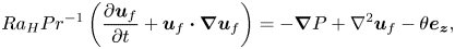
Geophysical problems considered here involve convective systems driven by internal heating and secular cooling, phenomena that are mathematically equivalent. Thermal convection in the Boussinesq approximation is governed by the following equations representing the conservation of momentum, energy and mass (see, e.g. Jaupart & Mareschal Reference Jaupart and Mareschal2010, p. 114):
 $$\begin{gather} \rho_{0,f} \left(\frac{\partial \boldsymbol{u}_{f}}{\partial t}+\boldsymbol{u}_{f} \boldsymbol{\cdot} \boldsymbol{\nabla} \boldsymbol{u}_{f}\right) ={-} \boldsymbol{\nabla} P + \eta_{f} \nabla^{2} \boldsymbol{u}_{f} - \alpha_{f} \rho_{0,f} \theta \boldsymbol{g}, \end{gather}$$
 $$\begin{gather}\rho_{0,f} c_{p,f} \left(\frac{\partial T}{\partial t}+ \boldsymbol{u}_{f}\boldsymbol{\cdot} \boldsymbol{\nabla} T\right)=\lambda_{f} \nabla^{2} T + H, \end{gather}$$
 $$\begin{gather}\boldsymbol{\nabla} \boldsymbol{\cdot} \boldsymbol{u}_{f}=0, \end{gather}$$
where  $\boldsymbol {u}_{f}$ is the fluid velocity field,
  $\rho _{0,f}$ is the reference fluid density,
  $\eta _{f}$ is its dynamic viscosity,
  $\alpha _{f}$ is its thermal expansion,
  $c_{p,f}$ is its specific heat,
  $\lambda _{f}$ is its thermal conductivity,
  $\boldsymbol {g}$ is the acceleration due to gravity,
  $H$ is the rate of internal heat generation,
  $P$ is the pressure,
  $T$ is the temperature field and
  $\theta =T-\langle T\rangle$ is the thermal anomaly with
  $\langle T\rangle$ the horizontal average temperature.
Internally heated convective systems are characterized by the internal temperature scale  $\Delta T_{H}$ defined as
 \begin{equation} \Delta T_{H}=\frac{Hh^{2}}{\lambda_{f}}, \end{equation}
where  $h$ is the vertical thickness of the system. This temperature scale introduces a new definition of the Rayleigh number, called the Rayleigh–Roberts number (Roberts Reference Roberts1967)
 \begin{equation} Ra_{H}=\frac{\alpha_{f} \rho_{0,f} g Hh^{5}}{\eta_{f} \kappa_{f} \lambda_{f}}, \end{equation}
where  $\kappa _{f}=\lambda _{f}/\rho _{0,f}c_{p,f}$ is the fluid's thermal diffusivity. This dimensionless number enables the characterization of the vigour and patterns of convection (e.g. Vilella et al. Reference Vilella, Limare, Jaupart, Farnetani, Fourel and Kaminski2018).
Using  $h$ as the length scale,
  $\Delta T_{H}$ as the temperature scale,
  $W=\rho _{0,f}\alpha _{f}g\Delta T_{H} h^{2}/\eta _{f}$ as the velocity scale that represents the Stokes velocity of a laminar thermal,
  $h/W$ as the time scale and
  $\eta _{f}W/h$ as the pressure scale, one can provide dimensionless form of the Boussinesq equations as follows (see, e.g. Jaupart & Mareschal Reference Jaupart and Mareschal2010, p. 114):
 $$\begin{gather} Ra_{H} Pr^{{-}1}\left(\frac{\partial \boldsymbol{u}_{f}}{\partial t}+\boldsymbol{u}_{f} \boldsymbol{\cdot} \boldsymbol{\nabla} \boldsymbol{u}_{f}\right) ={-} \boldsymbol{\nabla} P + \nabla^{2} \boldsymbol{u}_{f} - \theta \boldsymbol{e_{z}}, \end{gather}$$
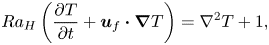 $$\begin{gather}Ra_{H} \left(\frac{\partial T}{\partial t}+ \boldsymbol{u}_{f}\boldsymbol{\cdot} \boldsymbol{\nabla} T\right)=\nabla^{2} T + 1, \end{gather}$$
 $$\begin{gather}\boldsymbol{\nabla} \boldsymbol{\cdot} \boldsymbol{u}_{f}=0, \end{gather}$$
where  $Pr$ is the Prandtl number, which compares viscous and thermal diffusion
 \begin{equation} Pr=\frac{\nu_{f}}{\kappa_{f}}, \end{equation}
where  $\nu _{f}=\eta _{f}/\rho _{f}$ is the kinematic viscosity. The Prandtl and Rayleigh–Roberts numbers characterize the regime of convection occurring in the system. They scale inertia in (2.6). The high-
 $Pr$ low-
 $Ra_{H}$ limit corresponds to laminar flows, whereas low-
 $Pr$ high-
 $Ra_{H}$ yields turbulent inertial flows. In geophysical systems, these dimensionless numbers span a large range of values. For instance, solid-state convection in the current Earth's mantle verifies
  $Pr\approx 10^{23}$ and
  $Ra\approx 10^{7}$, whereas magmatic reservoirs are rather evolving with
  $Pr\approx 10^{3}-10^{8}$ and
  $Ra\approx 10^{11}\text {--}10^{16}$. In the case of magma oceans, huge variation of
  $Pr$ and
  $Ra_{H}$ over the thermal history are expected. Massol et al. (Reference Massol2016) estimated for the terrestrial magma ocean a Rayleigh number that goes from
  $10^{31}$ at the very beginning if the planet is totally molten, to
  $10^{14}$ when crystals are in suspension. This drop can partly be explained by the fact that the presence of crystals increases the apparent viscosity of the mixture by several orders of magnitude when the rheological transition is reached (Lejeune & Richet Reference Lejeune and Richet1995; Guazzelli & Pouliquen Reference Guazzelli and Pouliquen2018). As a consequence, the
  $Pr$ number increases drastically during the solidification, from an initial value around
  $10^{1}\text {--}10^{2}$ to the current value of
  $10^{23}$ for solid mantle convection. In comparison, experiments carried out in the present study lie in the following ranges:
  $Pr\approx 10^{3}$ and
 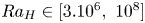 $Ra_{H}\in [3.10^{6},\ 10^{8}]$. According to the theory by Grossmann & Lohse (Reference Grossmann and Lohse2000), partially crystallized magma oceans and our experiments occur in the same regime of convection.
Internally heated convective systems are characterized by a single upper TBL generating cold instabilities. The temperature drop across the TBL  $\Delta T_{TBL}$ and the velocity of downwellings
  $W_{i}$ have been studied experimentally and numerically, and can be expressed based on local scaling analyses (Limare et al. Reference Limare, Vilella, Di Giuseppe, Farnetani, Kaminski, Surducan, Surducan, Neamtu, Fourel and Jaupart2015; Vilella et al. Reference Vilella, Limare, Jaupart, Farnetani, Fourel and Kaminski2018)
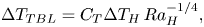 $$\begin{gather} \Delta T_{TBL}=C_{T}\Delta T_{H} \, Ra_{H}^{{-}1/4}, \end{gather}$$
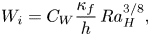 $$\begin{gather}W_{i}=C_{W}\frac{\kappa_{f}}{h} \, Ra_{H}^{3/8}, \end{gather}$$
where the pre-factors  $C_{T}$ and
  $C_{W}$ depend only on the mechanical boundary condition at the top of the system (see table 1).
Table 1. Pre-factors of scaling laws (2.10) and (2.11) determined numerically (Vilella et al. Reference Vilella, Limare, Jaupart, Farnetani, Fourel and Kaminski2018).

Introducing particles into the convective fluid adds significant complexity in the problem. Indeed, depending on the density, shape and size of the particles, but also depending on the fluid flow, multiple phenomena are likely to occur, which are described in an abundant literature (Andreotti, Forterre & Pouliquen Reference Andreotti, Forterre and Pouliquen2011; Boyer, Guazzelli & Pouliquen Reference Boyer, Guazzelli and Pouliquen2011; Houssais et al. Reference Houssais, Ortiz, Durian and Jerolmack2015). We summarize below the theoretical framework and fundamental parameters that will later be used to model these interacted phenomena.
2.2. Particles in suspension – two-phase flow
The presence of crystals dispersed in a magma reservoir makes it a two-phase system. To describe the dynamics of two-phase flow, a set of complementary equations has to be added to the conservation equations (2.1)–(2.3) to describe the two phases and the interactions between them (see, e.g. Andreotti et al. Reference Andreotti, Forterre and Pouliquen2011, p. 306). Considering the fluid phase ( $f$) and the solid phase (
 $p$), and assuming that the volume fraction
  $\phi$ of the solid phase is uniform, i.e. no chemical or mass exchanges between the phases, equations of motion for the fluid and the particles are, respectively,
 \begin{align} (1-\phi)\rho_{0,f}\left(\frac{\partial \boldsymbol{u}_{f}}{\partial t}+ \boldsymbol{u}_{f}\boldsymbol{\cdot}\boldsymbol{\nabla} \boldsymbol{u}_{f}\right)&={-}(1-\phi)\boldsymbol{\nabla} P+(1-\phi) \eta_{f} \nabla^{2} \boldsymbol{u}_{f}, \nonumber\\ &\quad -(1-\phi)\rho_{0,f}\alpha_{f}\theta\boldsymbol{g}-\boldsymbol{f}, \end{align}
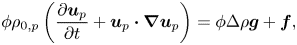 \begin{align} \phi \rho_{0,p}\left( \frac{\partial \boldsymbol{u}_{p}}{\partial t} +\boldsymbol{u}_{p}\boldsymbol{\cdot} \boldsymbol{\nabla} \boldsymbol{u}_{p}\right) &= \phi \Delta \rho \boldsymbol{g} +\boldsymbol{f}, \end{align}
where 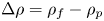 $\Delta \rho =\rho _{f}-\rho _{p}$ is the density difference between the fluid and the particles, and
  $\boldsymbol {f}$ is the fluid–particle interaction force. All other forces are neglected, such as Van der Waals interactions or frictional forces between particles. There are many approaches describing the interaction force
  $\boldsymbol {f}$ depending on the flow regime and particle properties (Maxey & Riley Reference Maxey and Riley1983). Here, we consider that, at high
  $Pr$ number, the interaction between the fluid and particles is dominated by the viscous drag, which is written as
 \begin{equation} \boldsymbol{f}=\beta(\phi)\frac{\eta_{f}}{r^{2}}(\boldsymbol{u}_{f} -\boldsymbol{u}_{p}), \end{equation}
where  $r$ is the particle radius and
  $\beta (\phi )$ is a dimensionless function that refers to the contribution of the other particles to the drag. It increases as
  $\phi$ increases (Andreotti et al. Reference Andreotti, Forterre and Pouliquen2011, p. 306).
Using the same scales as before, the dimensionless set of equations becomes
 $$\begin{gather} \frac{\partial \boldsymbol{u}_{f}}{\partial t}+\boldsymbol{u}_{f}\boldsymbol{\cdot}\boldsymbol{\nabla} \boldsymbol{u}_{f}=Ra_{H}^{{-}1}Pr(\boldsymbol{\nabla} P+\nabla^{2} \boldsymbol{u}_{f}-\theta\boldsymbol{e_{z}})- \frac{\beta(\phi)}{1-\phi}\frac{\rho_{0,p}}{\rho_{0,f}}St^{{-}1} (\boldsymbol{u}_{f}-\boldsymbol{u}_{p}), \end{gather}$$
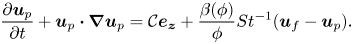 $$\begin{gather}\frac{\partial \boldsymbol{u}_{p}}{\partial t}+\boldsymbol{u}_{p}\boldsymbol{\cdot} \boldsymbol{\nabla} \boldsymbol{u}_{p}=\mathcal{C}\boldsymbol{e_{z}} + \frac{\beta(\phi)}{\phi}St^{{-}1}(\boldsymbol{u}_{f}-\boldsymbol{u}_{p}). \end{gather}$$
Two other dimensionless numbers appear. The  $\mathcal {C}$ parameter compares the gravitational potential energy of particles with the inertial drag
 \begin{equation} \mathcal{C}=\frac{\Delta \rho g h}{\rho_{0,p}W^{2}}. \end{equation}
In our experiments, this parameter is of order unity. The Stokes number characterizes the interaction between the fluid and particles
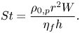 \begin{equation} St=\frac{\rho_{0,p}r^{2}W}{\eta_{f} h}. \end{equation}
For reservoirs much larger than the size of the particles, which is a limit relevant for magma oceans or magma reservoirs and/or for laminar flow, the Stokes number is likely to be much smaller than unity. In this case, particles are statistically passive tracers, following fluid motions (e.g. Crowe et al. Reference Crowe, Schwarzkopf, Sommerfeld and Tsuji2011, p. 25). Consequently, (2.16) becomes
 \begin{equation} \boldsymbol{u}_{p}=\boldsymbol{u}_{f}. \end{equation}
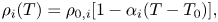
We emphasize that this limit describes the average behaviour of particles but does not imply that particles never settle. Over a short time scale compared with the convective time scale, the particles are indeed passive tracers and the equality (2.19) holds true. Nevertheless, particles are still buoyant, so there is a small component of the particle velocity that participates in settling. In this way, (2.19) rewrites  $\boldsymbol {u}_{p}=\boldsymbol {u}_{f} + \boldsymbol {u}_s$, with
 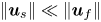 $\| \boldsymbol {u}_s\| \ll \| \boldsymbol {u}_f\|$. Thus, sedimentation actually occurs with a low probability (Patočka, Calzavarini & Tosi Reference Patočka, Calzavarini and Tosi2020), and deposits form at long time scales compared with the convective one.
A direct consequence of particles sedimentation is the formation of settled cumulates or floating lids. This implies in turn that erosion and particles re-entrainment from these layers must be taken into account in the modelling of convective systems.
2.3. Settling and re-entrainment
Erosion and re-entrainment from settled cumulates and/or floating lids bring particles back in suspension (Solomatov et al. Reference Solomatov, Olson and Stevenson1993). However, the framework that describes this phenomenon is different from the one used to treat suspensions as it depends on local mechanical equilibrium of the particles (Charru et al. Reference Charru, Mouilleron and Eiff2004; Lajeunesse et al. Reference Lajeunesse, Malverti and Charru2010). Particles at the surface of the bed are submitted to two forces: (i) the frictional force between the particles and the underlying bed that captures particles at the surface of the bed and is proportional to the particles buoyancy according to Coulomb's law and (ii) the shear stress induced by the flow. A dimensionless number, called the Shields number, compares these two forces (Shields Reference Shields1936)
 \begin{equation} \zeta=\frac{\tau}{\Delta \rho g r}, \end{equation}
where  $\tau$ is the shear stress at the surface of the bed. This ratio enables the definition of a critical value
  $\zeta _{c}$ that describes the threshold behaviour of particles on the bed. If
  $\zeta <\zeta _{c}$, particles are locked on the bed by frictional forces, whereas if
  $\zeta >\zeta _{c}$, the shear stress is strong enough to erode particles. For spherical plastic particles homogeneously sheared by a viscous, laminar flow, Charru et al. (Reference Charru, Mouilleron and Eiff2004) estimated
  $\zeta _{c}=0.12$.
The force driving particles (re-)entrainment does not take into account any vertical pressure effects. This follows the comment made by Solomatov et al. (Reference Solomatov, Olson and Stevenson1993) that a single particle cannot be lifted by a vertical pressure gradient by comparing the pressure force exerted on the particle with its buoyancy. The authors proposed that the mechanism for entrainment of particles is strongly linked to the shear stress acting at the interface, that manages to displace particles and forms dunes that enable entrainment.
The framework presented above can be used to describe the dynamics of a suspension and the coupled stability of cumulates and/or floating layers. To our knowledge, this coupling has not been studied yet in internally heated convective systems relevant for magma reservoirs. To fill this gap, we present below laboratory-scale experiments.
3. Experimental approach
3.1. Convection with internal heating
Achieving experimental convection driven by homogeneous internal heating at high Rayleigh numbers was challenging until Limare et al. (Reference Limare, Surducan, Surducan, Neamtu, di Giuseppe, Vilella, Farnetani, Kaminski and Jaupart2013) developed a unique experimental set-up based on microwave absorption. A  $30\times 30\ \mathrm {cm}^{2}$ wide and
  $5\ \mathrm {cm}$ high tank is introduced in a specially designed microwave oven (Surducan et al. Reference Surducan, Surducan, Limare, Neamtu and Giuseppe2014). The top of the tank is a thermostated aluminium plate whose temperature is fixed and monitored. The other walls and the base of the tank are made of poly(-methyl methacrylate) (PMMA), transparent to visible light and microwave radiation, and ensuring adiabatic thermal boundary conditions.
A laser sheet scans half of the tank ( $15\ \mathrm {cm}$), and we acquire images at a spacing of
  $1\ \mathrm {cm}$. Two CCD cameras register images in different spectral ranges allowing non-invasive measurement of the temperature field via a two-dye laser induced fluorescence method (LIF). The velocity field is measured by particle image velocimetry (PIV). The temperature and velocity spatial resolutions are
  $0.2$ and
  $0.8\ \mathrm {mm}$, respectively. Further details on the experimental set-up and calibration can be found in Fourel et al. (Reference Fourel, Limare, Jaupart, Surducan, Farnetani, Kaminski, Neamtu and Surducan2017). The same set-up and methods are used in the following study, but the fluid is adapted to study the sedimentation of beads. Typical two-dimensional velocity and temperature fields are shown in figure 1 for experiments without beads. Panels (a.1) and (b.1) show the two-dimensional horizontal and vertical velocity fields and their correspondent r.m.s. vertical profiles (panels (a.2) and (b.2)). The velocity is zero on the boundaries since they are all rigid. Negative vertical velocities are associated with thermal instabilities generated at the top boundary of the tank. Positive vertical velocities correspond only to return flow. Figure 1(c.2) displays the temperature vertical profile, showing that the thermal structure of the convective layer can be split into an upper boundary layer and a convective interior. An important feature is that the fluid interior has a slightly negative temperature gradient. This has been verified numerically (Sotin & Labrosse Reference Sotin and Labrosse1999; Vilella et al. Reference Vilella, Limare, Jaupart, Farnetani, Fourel and Kaminski2018) and experimentally (Limare et al. Reference Limare, Vilella, Di Giuseppe, Farnetani, Kaminski, Surducan, Surducan, Neamtu, Fourel and Jaupart2015).
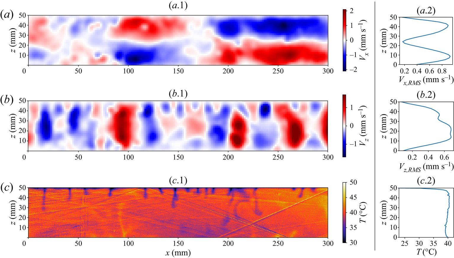
Figure 1. Two-dimensional horizontal velocity (a.1), vertical velocity (b.1) and temperature (c.1) fields for an experiment without beads ( $\rm {IHB29\_3}$). We display the corresponding root-mean-square (r.m.s.) vertical profiles for the horizontal and vertical velocity in (a.2) and (b.2) respectively, and the average temperature profile (c.2).
Table 2. Main physical properties of the fluid and beads. The activation energy is obtained from the viscosity fit with an Arrhenius law:  $\eta (T)=\eta _{f} \exp [({E_{a}}/{R})({1}/{T}-{1}/{T_{0}})]$, with
  $T_{0}=20\,^\circ \textrm {C}$. Properties are all measured in the laboratory, except those marked with (*) which are taken from Mark (Reference Mark2007). See supplementary material available at https://doi.org/10.1017/jfm.2021.862 for further information on the way property measurements have been carried out.
3.2. Fluid and particles
The working fluid used in experiments is a mixture of  $44\ \mathrm {wt}\,\%$ glycerol and
  $56\ \mathrm {wt}\,\%$ ethylene glycol. Particles are PMMA spherical beads. Two sets of beads are used, corresponding to two different radii (
 $r_{1}=290\ \mathrm {\mu }$m,
  $r_{2}=145\ \mathrm {\mu }$m). The main properties are summarized in table 2. Particles have a different thermal expansion coefficient
  $\alpha _{p}$ than the fluid, allowing the investigation of the full range of particle behaviours. For both phases, the density is linked to the temperature according to the thermal equation of state
 \begin{equation} \rho_{i}(T)=\rho_{0,i}[1-\alpha_{i}(T-T_{0})], \end{equation}
where  $T_{0}$ is the reference temperature,
  $\rho _{0,i}$ is the reference density at the reference temperature
  $T_{0}$ and
  $i$ refers to the fluid or particles. In this case, the density difference between the fluid and particles is
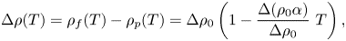 \begin{equation} \Delta \rho(T)=\rho_{f}(T)-\rho_{p}(T)=\Delta \rho_{0}\left(1-\frac{\Delta (\rho_{0}\alpha)}{\Delta \rho_{0}}\ T\right), \end{equation}
with  $\Delta (\rho _0 \alpha )=\rho _{0,f}\alpha _f-\rho _{0,p}\alpha _p$. If the fluid is cold enough, particles are lighter than the fluid and float, whereas at higher temperature, beads become heavier and can sink. Thus, an inversion of buoyancy exists at an ‘inversion temperature’
  $T_{{inv}}$ (figure 2). Furthermore, when the thermal state in the experimental tank spans a large range of temperatures, from the cold surface temperature
  $T_{{s}}< T_{{inv}}$ to the bulk temperature
  $T_{{bulk}}>T_{{inv}}$, the system can display simultaneously both a floating lid and cumulate formation. In our case,
 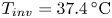 $T_{{inv}}=37.4\,^\circ \textrm {C}$.
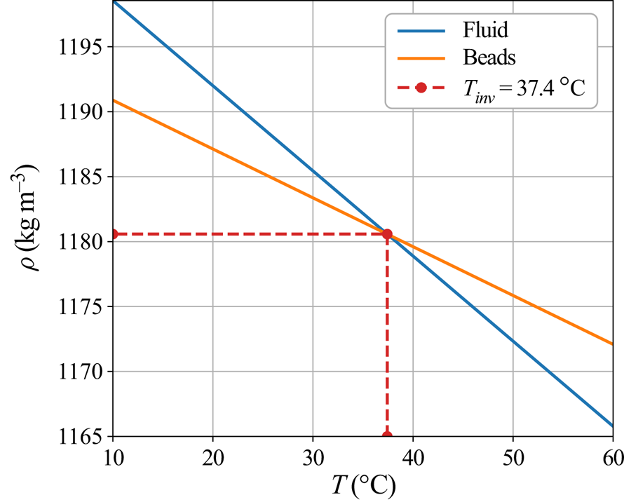
Figure 2. Variation of the density of the beads and the fluid with temperature. The range of temperatures reached in experiments ( $10\text {--}60\,^\circ \textrm {C}$) gives rise to both sinking and floating particle behaviours.
Experimental conditions are summarized in table 3. The fluid Prandtl number is high ( $Pr\approx 1000$) and experiments reached high Rayleigh–Roberts numbers (
 $Ra_{H}\in [3.10^{6},\ 10^{8}]$). The particle Stokes number is approximately
  $10^{-5}\text {--}10^{-4}$, which makes them passive tracers.
Table 3. Experimental characteristics: the beads’ radius  $r$, the initial floating bed thickness
  $\delta _{0}$, the imposed surface temperature
  $T_{s}$, the mean bulk temperature at steady state
  $T_{{bulk}}$, the Rayleigh–Roberts number calculated at steady state
  $Ra_{H}$. The two last columns inform about the erosion of the floating lid (whether partial or total), and the formation of a cumulate at the bottom of the tank. Note that two families of beads with different radii are used. The last 8 rows correspond to experiments done without beads.

As particles are made of PMMA, they are transparent to microwave radiation, so internal heating only occurs in the fluid. Comparing the diffusive time scale in one particle  $\tau _{d}\sim r^{2}/\kappa _{p}$ and the convective time scale
  $\tau _{c}\sim h/W$ leads to
 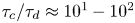 $\tau _{c}/\tau _{d}\approx 10^{1}-10^{2}$, which shows that the thermal equilibration of the particles is rapid. Thus, we assess that the local temperature difference between the particles and the fluid is negligible.
Unfortunately, in this configuration, we could not achieve refractive index matching between the beads and particles (see supplementary material). Consequently, plastic beads are light-scattering objects and the images recorded by the cameras are blurred. This has little influence on the velocity measurement, as particles behave like passive tracers. In order to check if it affects the temperature measurements, we carried out a sedimentation experiment using a homogeneous suspension in a controlled isothermal environment. We monitored the fluorescent signal whilst particles settled, and confirmed that the mean temperature measured was consistent with the imposed temperature. Hence, the presence of beads does not affect the measurement of the average properties of convection, on which further reasoning is based.
3.3. Experiments
Experiments were conducted as follows. The tank was filled with a mixture of fluid and particles. One has to avoid introducing air into the system, in order to limit surface tension effects (see supplementary materials for more details). The system is thermostated at the surface temperature  $T_{s}$ generally bellow
  $T_{{inv}}$, so that particles form initially a floating lid (see figure 3). Then, the microwave power is turned on and convection starts within a time lapse of a few tens of seconds. As convection proceeds, the floating lid is eroded, and particles are placed in suspension. In some experiments, the inversion temperature was reached, and particles could further form a cumulate (table 3). We waited until the thermal steady state was reached (which corresponds to a period of time spanning from 2 to 6 hours).
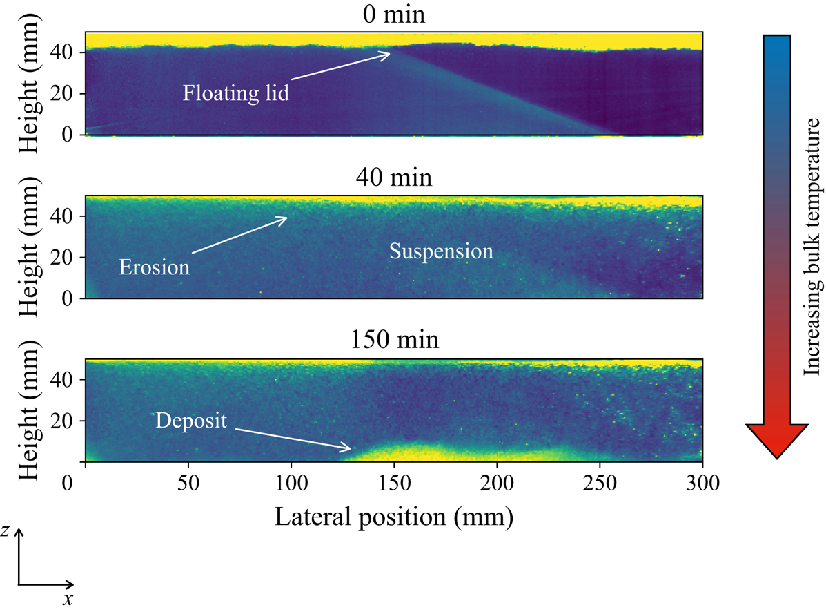
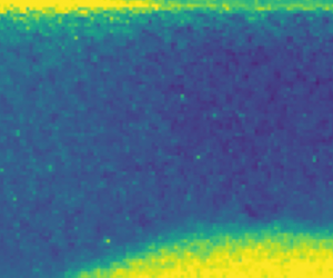
Figure 3. Snapshots of one cross-section ( $y=20\ \textrm {mm}$ from the tank front wall) during an experiment (IHB05), showing the typical phenomena observed. Images are taken at 3 different moments in time:
  $t=0, 40$ and
  $150\ \textrm {min}$ after the microwave power was turned on. Colours stand for the laser light intensity scattered. Blue colour corresponds to the fluid. Hotter colours correspond to beads. At
  $t=0$, convection begins, and particles are eroded from the floating lid. The erosion of the floating lid can be either partial or total depending on the experimental conditions (table 3). In some cases, due to progressive heating of fluid, beads become heavier than the fluid and settle to form a cumulate.
In the following section, we will study in detail these two aspects: the erosion of the floating lid and the formation of the cumulate.
4. Floating lid
4.1. Thermal steady state
The presence of a floating lid is likely to influence the thermal state of the system as it is situated in the TBL (figure 4). In the following section, we will quantify the thickness of the steady lid and the thermal state of the system.
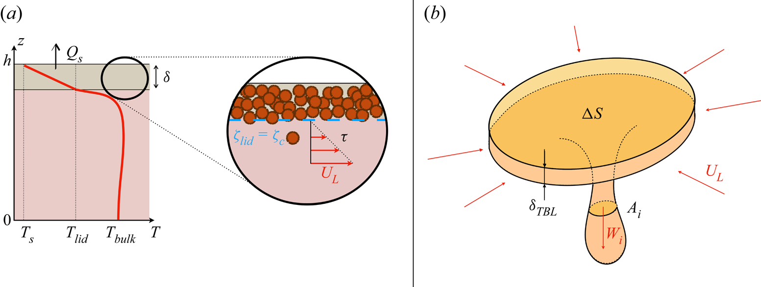
Figure 4. (a) Illustration of the thermal state of the system and of the erosion model used to determine the lid thickness at steady state, with  $h$ the reservoir thickness,
  $T_{s}$ the surface temperature,
  $T_{{lid}}$ the basal temperature of the floating lid,
  $T_{{bulk}}$ the average bulk temperature,
  $Q_{s}$ the surface heat flux,
  $\delta$ the floating lid thickness,
  $\zeta$ the Shields number defined in the text,
  $\zeta _{c}$ its critical value,
  $\tau$ the convective shear stress and
  $U_{L}$ the horizontal velocity scale. (b) Schematic view of a downwelling used for the shear stress scaling law. Here,
  $\Delta S$ stands for the surface from which the fluid is drained,
  $\delta _{TBL}$ is the TBL thickness,
  $W_{i}$ the maximal velocity of cold plumes.
Figure 5 reveals that the dimensionless drop of temperature between the bulk and the surface is systematically higher than the one predicted by the scaling laws (2.10). We displayed the scalings for both mechanical conditions (rigid and free slip) since this boundary condition is not well defined beneath a granular lid. The lid reduces the efficiency of heat transfer that occurs at the top of the reservoir and causes an insulating effect related to the lid thickness.
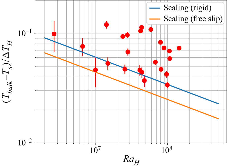
Figure 5. Experimental dimensionless drop of temperature  $(T_{{bulk}}-T_{s})/\Delta T_{H}$ as a function of the Rayleigh–Roberts number at steady state. The two solid lines stand for scaling laws for homogeneous internal heating with rigid and free-slip top conditions:
  $(T_{{bulk}}-T_{s})/\Delta T_{H}=C_{T} \, Ra_{H}^{-1/4}$ where
  $C_{T}$ is given table 1.
To quantify this effect, we use the model developed to study convection under a conductive lid (Guillou & Jaupart Reference Guillou and Jaupart1995; Lenardic & Moresi Reference Lenardic and Moresi2003; Grigné et al. Reference Grigné, Labrosse and Tackley2007). The reasoning is based on two hypotheses. First, we consider the lid as a homogeneous conductive layer with an average conductivity  $\bar {\lambda }$, and an averaged thickness
  $\delta$, such that the heat flow through the lid is
 \begin{equation} Q_{s}=\bar{\lambda} \frac{T_{{lid}}-T_{s}}{\delta_{{th}}}, \end{equation}
where  ${T_{{lid}}}$ is the basal temperature of the lid and
  $Q_{s}=Hh$ is the surface heat flux at steady state. The lid's mean conductivity is estimated based on the individual values of each component weighted by their respective volume fraction
  $\bar {\lambda }=\phi _{{RLP}}\lambda _{p}+(1-\phi _{{RLP}})\lambda _{f}$, with
  $\phi _{{RLP}}$ the beads packing in the lid, assumed to be the random loose one:
  $\phi _{RLP}=56\,\%$. We further consider that the scaling laws for thermal convection hold true beneath the conducting lid. It has been verified experimentally for homogeneous internally heated systems that the drop of temperature between the surface and the bulk
  $T_{{bulk}}-T_{s}$ scales like the drop of temperature through the TBL
  $\Delta T_{TBL}$ given in (2.10) with a pre-factor
  $C_{T}=3.38\pm 0.16$ at steady state (Limare et al. Reference Limare, Jaupart, Kaminski, Fourel and Farnetani2019). Thus, thanks to the continuity of temperature between the lid and the fluid, one can get
 \begin{equation} T_{{bulk}}= T_{{lid}}+C_{T}\Delta T_{H}\, Ra_{H}^{{-}1/4}, \end{equation}
which combined with (4.1) yields
 \begin{equation} \frac{\delta_{{th}}}{h}=\frac{\bar{\lambda}}{\lambda_{f}} \left(\frac{T_{{bulk}}-T_{{s}}}{\Delta T_{H}}-C_{T}\, Ra_{H}^{{-}1/4}\right),\end{equation}
showing that the larger the lid thickness, the hotter the bulk.
To validate this model, which uses the thermal state of the system to estimate the lid thickness, an independent way to measure  $\delta$ is required. In that aim we explore the r.m.s. velocity field. Figures 6(
 $a.1$) and 6(
 $a.2$) highlight the shape of r.m.s. velocity profiles for a convective fluid in the absence of particles. Because of rigid boundary conditions, velocities vanish at the surface and at the floor of the reservoir. Consequently, by symmetry, the vertical velocity field has a maximum value at mid-depth – figure 6(
 $a.2$). Also by symmetry, the horizontal profiles have a minimum value at mid-depth between two maxima corresponding to
  $1/4$ and
  $3/4$ of the total thickness of the tank, as can be seen in figure 6(
 $a.1$). This shape is due to the confined environment that creates a horizontal recirculation flow. As emphasized in figures 6(
 $b.1$) and 6(
 $b.2$), the presence of the floating lid shifts vertically the point where the horizontal velocity is minimal by an amount
  $\Delta \delta$, which is set by the ‘mechanical’ thickness of the lid
  $\delta _{m}$
 \begin{equation} \Delta \delta=\frac{\delta_{m}}{2}. \end{equation}
Comparison between the thickness deduced from the velocity-shift method  $\delta _{m}$ and the inverted thermal thickness
  $\delta _{{th}}$ calculated thanks to (4.3) is shown in figure 7. In this plot, we only use experiments where the lid is partially eroded and where no cumulate appears at steady state, in order to limit unwanted shifts due to the presence of a deposit of particles at the base of the tank. The agreement between the measurements and the model is fair, despite some scatter due to the simplifications of the model used. We assessed that the floating lid can be approximated by a homogeneous conductive lid whilst it is composed of packed particles containing interstitial fluid. Moreover, its thickness is not strictly uniform as dunes form during erosion/deposition processes (see supplementary materials). In the following, we will use the thermal thickness
  $\delta _{{th}}$ to characterize the lidthickness.
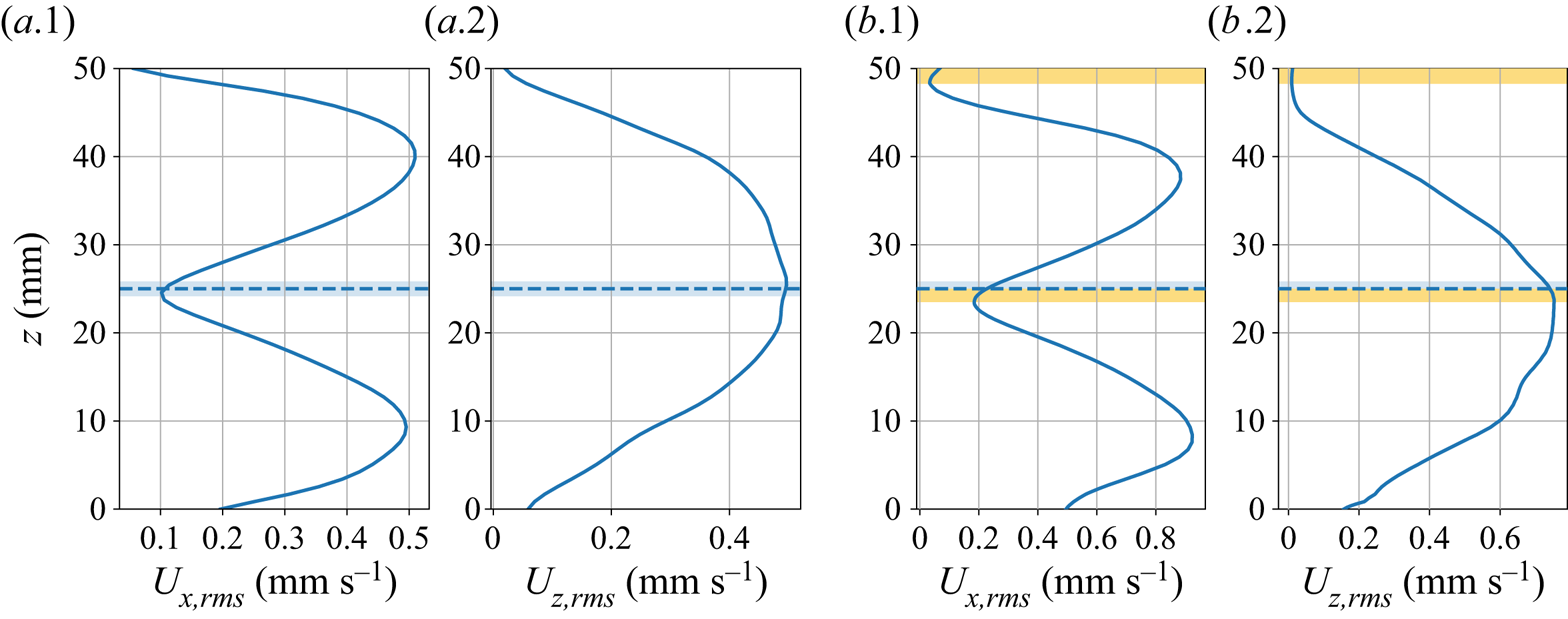
Figure 6. The r.m.s. horizontal and vertical velocity values at steady state, averaged at each depth  $z$ for an experiment without beads (a) and with a floating lid (b). The mid-depth of the tank is represented by the dashed line. In the case (b), the depth at which the local extremum of the velocity is shifted, because of the floating lid schematized by the yellow bands.
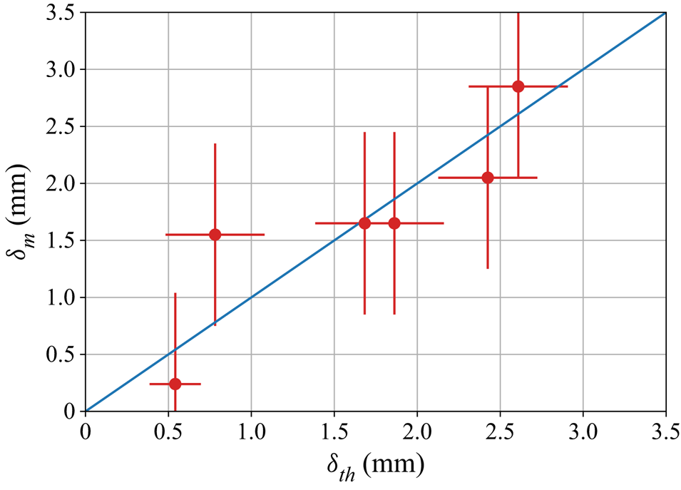
Figure 7. Comparison between the lid thickness inverted from the thermal state  $\delta _{{th}}$ and the one measured by the velocity-shift method
  $\delta _{m}$. Error bars on
  $\delta _{m}$ correspond to one pixel of the PIV grid, and those on
  $\delta _{{th}}$ correspond to one particle radius.
Besides, the symmetry observed in the horizontally averaged vertical profile  $U_{x,rms}$ is clearly related to the return flow due to the rigid lateral boundaries and is not a general feature of convection driven by internal heating. For instance, in the case of a spherical shell, this symmetry has a priori no reason to exist. This experimental feature was used as an additional measurement of the floating lid thickness. This assumption does not affect the validity of the reasoning as our model does not require a symmetry of the lateralflow.
4.2. Predictive model for the floating lid
4.2.1. Local mechanical equilibrium
As illustrated in figure 4(a), local equilibrium of the beads is set by the balance between erosion forces and the bead buoyancy. To quantify such an equilibrium, we rely on the threshold theory of mechanical erosion (Glover & Florey Reference Glover and Florey1951; Métivier, Lajeunesse & Devauchelle Reference Métivier, Lajeunesse and Devauchelle2017) and we define the Shields number  $\zeta _{{lid}}$ at the base of the floating lid as
 \begin{equation} \zeta_{{lid}}=\frac{\tau}{\Delta \rho(T_{{lid}})gr}, \end{equation}
where  $\tau =\eta _{f} \dot \gamma$ is the characteristic convective shear that acts on the bottom of the lid, and
  $\dot \gamma$ the corresponding strain rate. We consider only the experiments with partial erosion of the floating lid at steady state, which means that the lid thickness
  $\delta \neq 0$. In these experiments, the Shields number reaches the critical threshold (
 $\zeta _{{lid}}=\zeta _{c}$ in (4.5) and
  ${\delta =\delta _{{th}}}$ in (4.1)). At steady state, we assume that the temperature field in the floating lid varies linearly with depth, so that the temperature at the base of the lid is
 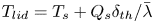 ${T_{{lid}}=T_s+Q_s \delta _{{th}} /\bar \lambda}$. Introducing this temperature in (3.2), some algebra yields the following set of equations:
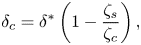 $$\begin{gather} \delta_{c}=\delta^{*}\left(1-\frac{\zeta_{s}}{\zeta_{c}}\right), \end{gather}$$
 $$\begin{gather}\delta^{*}=\frac{\Delta \rho (T_{s})}{\Delta (\rho_{0}\alpha)} \frac{\bar{\lambda}}{Q_{s}}, \end{gather}$$
 $$\begin{gather}\zeta_{s}=\frac{\tau}{\Delta \rho(T_{s})gr}, \end{gather}$$
where  $\zeta _{s}$ is the Shields number calculated at the surface temperature
  $T_{s}$. With (4.6),
  $\zeta _s$ appears as the control parameter that determines the critical thickness
  $\delta _{c}$, as
  $T_{s}$ and
  $Q_{s}$ are known. The problem thus boils down to the determination of the characteristic convective shear stress
  $\tau$. For instance, in experiments done by Charru et al. (Reference Charru, Mouilleron and Eiff2004), the shear is experimentally controlled and homogeneously applied to the bed, which facilitatesits characterization. Here, the bed lies in the unstable cold TBL. Thus the flow field is complex and contains spatial and temporal fluctuations. Hence, characterizing the shear stress in a homogeneously heated convective system is required.
4.2.2. Scaling laws for velocities and shear stresses
Equation (4.5) emphasizes the importance of the horizontal shear stress, hence of the velocity field, for the erosion process. The strain rate  $\dot \gamma$ scales as follows:
 \begin{equation} \dot \gamma \sim \frac{U_{L}}{\delta_{v}}, \end{equation}
where  $U_{L}$ is the characteristic horizontal velocity, and
  $\delta _{v}$ is the characteristic length over which velocity vanishes. By definition, the latter corresponds to the dynamical boundary layer (DBL) thickness. First, the Reynolds numbers
  $Re$ reached in our experiments are low, which implies laminar flows and thus
  $\delta _{v}\sim h$ (see Appendix A). As a consequence, the strain rate
  $\dot \gamma$ becomes
 \begin{equation} \dot \gamma \sim \frac{U_{L}}{h}. \end{equation}
We consider the volume of fluid in the TBL that is drained by one downwelling (figure 4b). On one side, fluid from the TBL is drained at the characteristic velocity  $W_{i}$ by the downwelling whose cross-sectional area is
  $A_{i}$. On the other hand, fluid is converging at the characteristic horizontal velocity
  $U_{L}$ through the lateral surface of the cylinder of thickness
  $\delta _{TBL}$ and area
  $\Delta S$. This reasoning is based on the fact that the fluid drained in one downwelling comes mainly from the TBL. This assumption is valid at the high Prandtl number limit where entrainment between downwellings and the ambient fluid is negligible (Davaille & Vatteville Reference Davaille and Vatteville2005). Mass conservation imposes
 \begin{equation} U_{L}\delta_{TBL}\Delta S^{1/2}\sim W_{i}A_{i}. \end{equation}
Using the same scalings as in Vilella et al. (Reference Vilella, Limare, Jaupart, Farnetani, Fourel and Kaminski2018)  $\delta _{TBL}\sim hRa_{H}^{-1/4}, \Delta S \sim h^{2} \, Ra_{H}^{-1/4}, A_{i}\sim h^{2}\, Ra_{H}^{-3/8}, W_{i}\sim \kappa _{f}/h\ Ra_{H}^{3/8}$, valid for
  $10^{6} \leq Ra_{H}\leq 10^{9}$, we obtain the horizontal velocity scale
 \begin{equation} U_{L}=C_{u} \frac{\kappa_{f}}{h}\, Ra_{H}^{3/8}, \end{equation}
with  $C_{u}$ a pre-factor which depends on the boundary conditions.
To verify these scaling laws, experiments without beads have been carried out using the same fluid and the same methods as those described previously. We recorded the horizontal and vertical velocities using the PIV method, and we calculated the horizontal and vertical strain rate. As we are interested in the average shear rate, we determined their r.m.s. values calculated over the entire volume of the tank. Results are displayed in figures 8(a) and 8(b) for the horizontal and vertical velocities. The scaling law pre-factors determined experimentally are summarized in table 4. In our experiments,  $Re\approx 10^{-1}-1$, so the convection is laminar.

Figure 8. Scaling laws derived from experiments without beads. Horizontal (a) and vertical (b) velocity, horizontal (c) and vertical (d) strain rate. All these physical properties are evaluated thanks to their r.m.s. values calculated in the entire volume of the tank and are represented by the dots. Blue lines represent best fit laws with fixed exponent  $3/8$ and the orange dashed line are those with the exponent left to vary. All parameters of these laws are summarized in table 4.
Table 4. Parameters of power laws determined experimentally for the horizontal and vertical r.m.s. velocities and the horizontal and vertical r.m.s. shear rates.
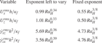
The scaling law for the strain rate is therefore  $C_{\gamma }({\kappa _{f}}/{h^{2}}) \, Ra_{H}^{3/8}$. Results are displayed in figures 8(c) and 8(d) for the horizontal and vertical strain rates, respectively. In both cases, the predicted scaling law is in good agreement with experimental data.
We can thus estimate the Shields number as follows:
 \begin{equation} \zeta_{s}=\frac{\eta_{f} \kappa_{f}}{h^{2}\Delta \rho(T_{s}) g r} \, Ra_{H}^{3/8}. \end{equation}
4.2.3. Critical shields number and stability of deposits
Thanks to the previous scaling analyses, (4.6) provides a way to measure experimentally the critical Shields number. By considering that the lid thickness at steady state corresponds to the critical thickness  $\delta _{{th}}=\delta _{c}$, one can determine the critical Shields number
  $\zeta _{c}$ for each experiment
 \begin{equation} \zeta_{c}=\zeta_{s}\left(1-\frac{\delta_{{th}}}{\delta^{*}}\right)^{{-}1}, \end{equation}
with  $\zeta _{s}$ given by (4.13). The critical number is calculated for each experiment, and results are displayed in figure 9. We obtain
  $\zeta _{c}=0.29 \pm 0.17$. This value is of the same order of magnitude of the one estimated by Charru et al. (Reference Charru, Mouilleron and Eiff2004). Error bars represent a variation of one bead radius of the floating lid thickness. The discrepancy is due to the sensitivity of the prediction to the value of the lid thickness, and the higher the heat flux, the steeper the thermal gradient in the lid and the greater the error bars. This is the reason why one experiment in particular (IHB13) does not appear in the plot because the uncertainties are too large.
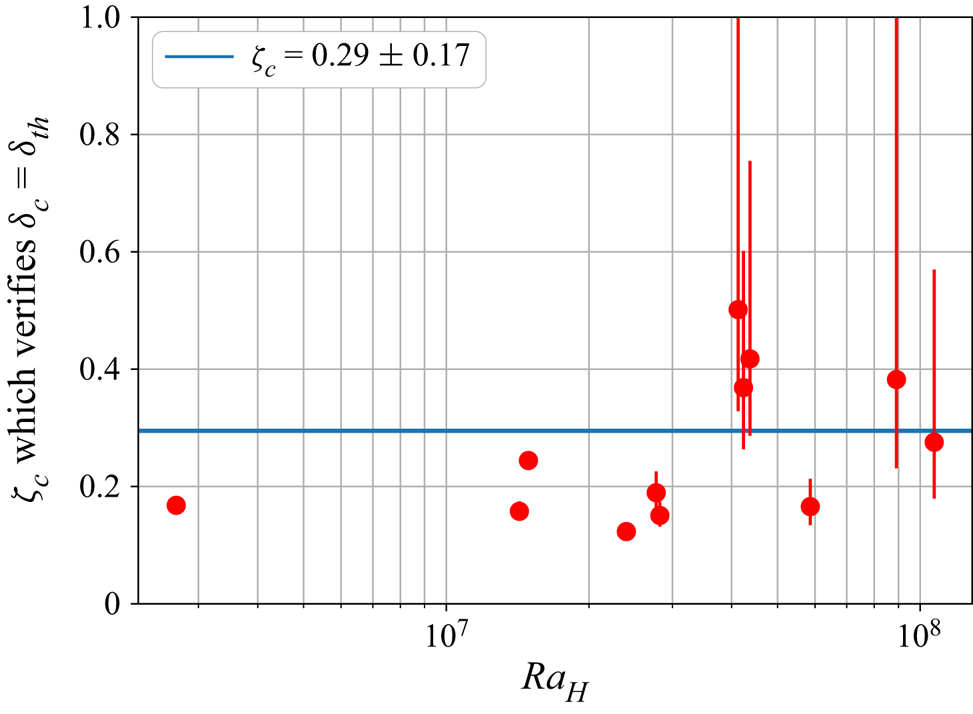
Figure 9. Determination of the critical Shields number  $\zeta _{c}=0.29 \pm 0.17$ to achieve a perfect match between the reference lid thickness
  $\delta _{{th}}$ and the critical thickness
  $\delta _{c}$.
With the critical number  $\zeta _{c}$ determined, we can compare the stability of the different deposits predicted by the Shields approach with the experimental observations (figures 10a and 10b). For the floating lid, we calculate the surface Shields number
  $\zeta _{s}$. If
  $\zeta _{s}>\zeta _{c}$, the floating lid is unstable and erosion should be total. But if
  $\zeta _{s}<\zeta _{c}$, a floating lid of some thickness is stable. Results are displayed in figure 10(a) and the transition between total erosion and partial erosion is well described by
  $\zeta _{c}$. Similarly, we calculate the bulk Shields number
  $\zeta _{{bulk}}$, which is also the Shields number at the base of the reservoir
 \begin{equation} \zeta_{{bulk}}=\frac{\eta_{f} \kappa_{f}}{h^{2}\Delta \rho(T_{{bulk}}) g r} \, Ra_{H}^{3/8}, \end{equation}
and we compare it with  $\zeta _{c}$. If
  $\zeta _{{bulk}}>\zeta _{c}$, convection prevents deposition at the base of the tank. Otherwise, a basal deposit is stable. This transition is also verified experimentally in figure 10(b).
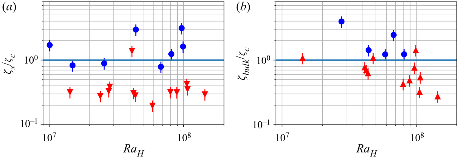
Figure 10. Stability of different deposits. (a) Stability diagram for the floating lid, based on the value of  $\zeta _{s}=\zeta (T_{s})$. Circles: the lid is totally eroded. Downward-pointing triangles: a stable lid is observed at steady state. (b) Stability of the cumulates that is likely to form when
  $T_{{bulk}}>T_{{inv}}$. This stability is compared with the value of the local Shields number at the bottom of the tank
  $\zeta _{{bulk}}=\zeta (T_{{bulk}})$. Circles: no deposit at steady state. Upward-pointing triangles: a cumulate is observed at steady state.
5. Suspension stability
The scalings derived above allow prediction of whether a deposit can form at the base of the reservoir and a stable lid at the top of it, but we need another framework to describe the full dynamics of the suspension containing the particles eroded from the deposits. In a fluid at rest, particles with negative buoyancy will all eventually settle down. Observations show that in a convective fluid, even negatively buoyant particles can remain in suspension at steady state (Lavorel & Le Bars Reference Lavorel and Le Bars2009). Solomatov & Stevenson (Reference Solomatov and Stevenson1993) proposed that the dynamics of the suspension can be described based on the equilibrium between buoyancy and shear forces, described by the balance
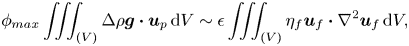 \begin{equation} \phi_{max} \iiint_{(V)}\Delta \rho \boldsymbol{g}\boldsymbol{\cdot}\boldsymbol{u}_{p}\, \mathrm{d}V \sim \epsilon \iiint_{(V)}\eta_{f} \boldsymbol{u}_{f}\boldsymbol{\cdot} \nabla^{2} \boldsymbol{u}_{f}\, \mathrm{d}V, \end{equation}
or in compact form,
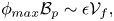 \begin{equation} \phi_{max}\mathcal{B}_{p} \sim \epsilon \mathcal{V}_{f}, \end{equation}
where  $\mathcal {B}_{p}$ is the integral on the left-hand side of (5.1) related to beads buoyancy,
  $\mathcal {V}_{f}$ is the integral on the right-hand side of (5.1) referring to the bulk viscous dissipation,
  $(V)$ is the total volume of the reservoir and
  $\epsilon$ is the percentage of viscous energy being used to maintain particles in suspension (also called the efficiency parameter). This description can be further used to determine the maximal concentration of particles
  $\phi _{{max}}$ that can be maintained in suspension by convection. Assuming
  $\epsilon$ to be constant, Solomatov & Stevenson (Reference Solomatov and Stevenson1993) get the following law for
  $\phi _{max}$:
 \begin{equation} \phi_{{max}}= C_{s}\epsilon \left(\frac{\bar{\tau}}{\overline{\Delta \rho} g r}\right)^{2}=C_{s} \epsilon \bar \zeta^{2}, \end{equation}
where  $\bar {\tau }$ and
  $\overline{\Delta \rho }$ stand for the volume averaged values of
  $\tau$ and
  $\Delta \rho$, respectively, and
  $C_{s}=9/2$ (Solomatov & Stevenson Reference Solomatov and Stevenson1993). Basically, if the concentration of particles in the convective bulk
  $\bar \phi$ is below this limit, particles stay in suspension. Otherwise, the convective fluid only sustains the quantity of particles corresponding to the maximal concentration
  $\phi _{max}$, and the rest settle, forming a cumulate. Interestingly, this law can be expressed with a Shields parameter
  $\bar \zeta$ similar to the one used previously. The major difference lies in the fact that
  $\bar \zeta$ is a global parameter, comparing volume average properties, whereas previously
  $\zeta$ has been estimated locally. However, by neglecting the thin TBL at the top of the reservoir, one can approximate that
 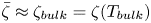 $\bar \zeta \approx \zeta _{{bulk}}=\zeta (T_{{bulk}})$, and thus
  $\phi _{{max}}$ is described by previous scaling laws.
In order to verify the validity of this criterion in our experiments, we considered the formation of the cumulate at the base of the tank. As the direct measurement of particle concentration  $\phi$ is not possible due to the refractive index mismatch, we calculate a proxy
  $\varphi$ of the quantity of particles eroded from the floating lid. To do so, taking
  $\delta _{0}$ as the initial thickness of the bed, and
  $\delta _{{th}}$ as the thickness at steady state, the quantity of particles that are eroded is proportional to
  $\delta _{0}-\delta _{{th}}$. The coefficient of proportionality is linked to the packing of particles inside the floating lid. The packing is assumed to be constant, as all experiments are prepared similarly. Thus, the concentration of particles in the bulk is calculated as if all the eroded material stays in suspension
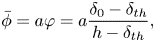 \begin{equation} \bar \phi=a\varphi =a\frac{\delta_{0}-\delta_{{th}}}{h-\delta_{{th}}}, \end{equation}
where  $a$ is a constant which depends potentially on the packing of beads inside the lid (
 $a=0.56$ for a random loose packing). As the measurement of the total quantity of deposit particles is subject to large uncertainties, we detect
  $\phi _{{max}}$ as the limit between partial sedimentation and absolute suspension defined by the limit
  $\phi _{{max}}\sim \overline {\zeta }^{2}$. The blue line in figure 11 represents the empirical boundary between the two regimes. Now, we have a complete framework that describes the steady state of any suspension in a convective environment driven by internal heating. The Shields formalism enables us to quantify the thickness of the lid located in a boundary layer, and Solomatov's approach enables us to describe the maximal quantity of particles that can stay in suspension.
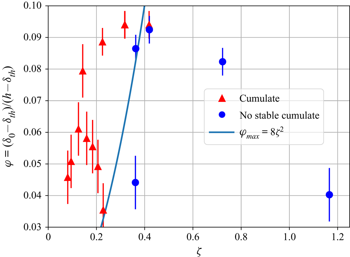
Figure 11. Proxy of particle concentration at steady state for all experiments where particles in suspension are heavier than the fluid. The blue line represents the transition between the cumulate regime et the absolute suspension one, assuming a constant efficiency coefficient.
6. Lid formation in a convective system bearing particles
Our results can be used to describe the fate of particles in a convective fluid by splitting the system into three reservoirs: (i) the floating lid situated in the TBL, (ii) the bulk fluid containing suspended particles and (iii) the deposit at the base. Our model quantifies the volume of particles that can be stored in each reservoir (figure 12). Buoyant crystals first fill the floating lid reservoir. We can define the maximal capacity of the floating lid  $V_{c}$ determined by (4.6). Particles exceeding this critical volume of the lid remain in suspension or form a cumulate. In the same way, for negatively buoyant crystals, if the bulk Shields number is below the critical value, a deposit may form. The concentration of crystals that stay in suspension is limited to
  $\phi _{{max}}$, the rest settle and form the basal deposit.
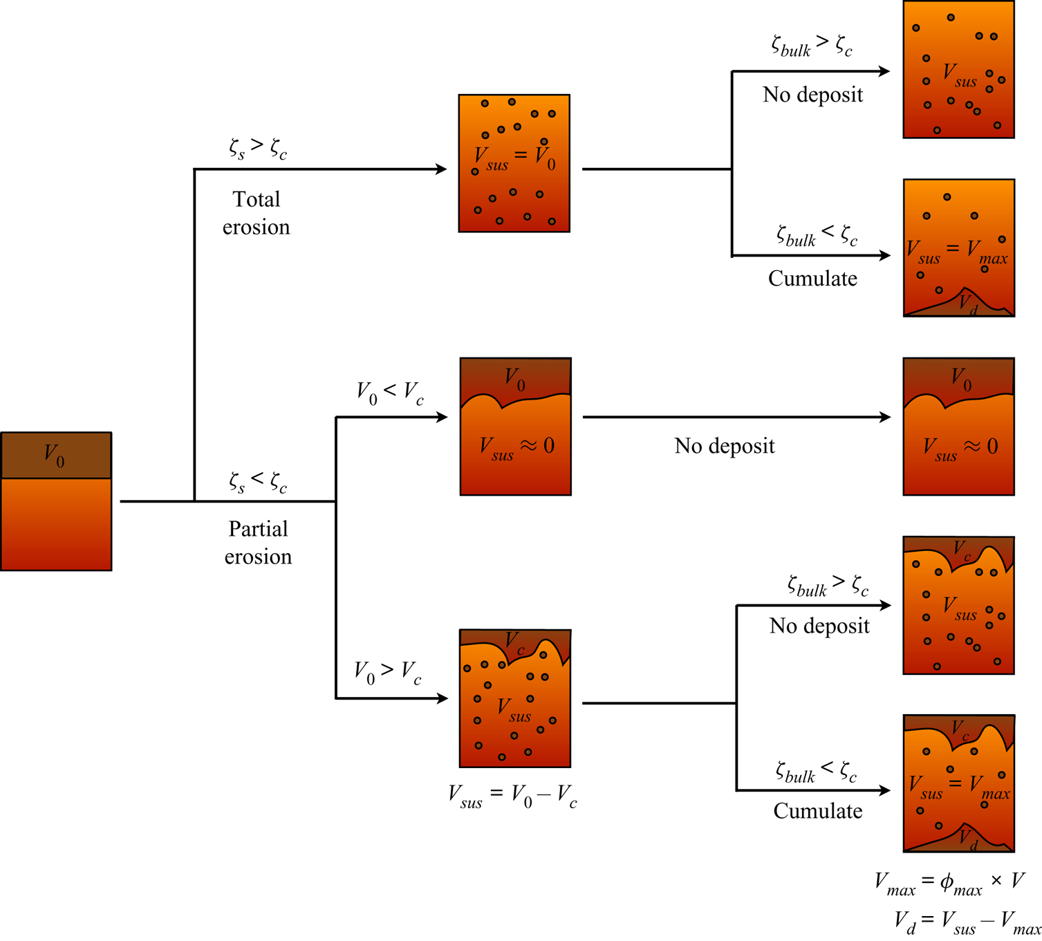
Figure 12. Synopsis that fully determines the system's regime at steady state. The surface Shields number  $\zeta _{s}$ is given by (4.13) and depends on the surface temperature
  $T_{s}$, the Rayleigh–Roberts number
  $Ra_{H}$ and the initial volume of particles
  $V_{0}$ which are all input parameters. Here,
  $V_{c}$ is the volume of the critical floating lid that can form at the surface of the convective fluid, corresponding to a lid of thickness
  $\delta _{c}$ given by (4.6). Stability of the floating lid: if
  $\zeta _{s}>\zeta _{c}$, the floating lid is unstable and all particles are placed in suspension. If
  $\zeta _{s}<\zeta _{c}$, the erosion is partial. In this case, if
  $V_{0}< V_{c}$, the initial crust is stable, and very few particles are placed in suspension. If
  $V_{0}>V_{c}$, only a volume of particles
  $V_{c}$ stays at the surface, the rest of the volume
  $V_{{sus}}=V_{0}-V_{c}$ is placed in suspension. Cumulate formation: we consider the stability of the suspension in the case of negatively buoyant suspended particles. If the basal Shields number
  $\zeta _{{bulk}}$ is greater than
  $\zeta _{c}$, the suspension is stable and no cumulate forms. If
  $\zeta _{{bulk}}>\zeta _{c}$, a basal cumulate can settle down. The volume of this cumulate is given by the maximal concentration of particles that can stay in suspension
  $\phi _{{max}}$ given by (5.3). The convective fluid can only sustain a maximal volume
  $V_{{max}}=\phi _{{max}} V$ in suspension, where
  $V$ is the volume of the convective layer;
  $V_{{max}}$ has to be compared with the volume of particle that have been eroded
  $V_{{sus}}$. The surplus
  $V_{d}=V_{{sus}}-V_{{max}}$ forms a basal cumulate.
7. Discussion
7.1. Validity of the experimental results
The approach adopted here takes into account the main mechanisms that deal with suspension and deposit stability. The main goal was to highlight how to use the framework treating of fluid/crystal interaction in the case of convective systems bearing crystals. It is based on hypotheses that allow us to express the problem in terms of scaling laws that can easily be re-scaled to conveniently describe a geophysical system as it will be illustrated in next section.
Even though experimental results are well described by our models at first order, certain discrepancies exist and should not be ignored. They result from different factors. First, our experiments enable the estimation of the floating lid thickness by an indirect measurement based on the average temperature state of the system. This method might increase the uncertainty on the determination of  $\delta$ and, thus, all parameters that are linked to it, such as the entrainment threshold. One way to improve this measurement could be the use of fluid and beads that have a near-perfect optical index matching. In this way, the bottom of the lid would be directly observable, and the thickness measurable more precisely. This prerequisite enabled the study of the bed surface motions and even of the motions of beads inside a granular bed (Mouilleron, Charru & Eiff Reference Mouilleron, Charru and Eiff2009; Houssais et al. Reference Houssais, Ortiz, Durian and Jerolmack2015). In this way, the bottom of the lid will be directly observable, and the thickness measurable more precisely.
Second, our theory is based on averaged physical properties, which leads to the general predicament of describing a three-dimensional problem by a one-dimensional theory. This crude approximation leads to results that are fairly consistent with data at first order, but a local description of the convection and the erosion mechanism can improve this approach. Downwellings develop from the TBL, which can have an influence on the local behaviour of beads at the bottom of the floating lid. Equivalently, we describe the floating lid as a quiescent solid medium of homogeneous thickness, but this assumption is a strong simplification. We point out the existence of a topography (see supplementary materials) that can have an influence on the local flow in the TBL, which, in turn, impacts the erosion mechanism that occurs at the interface (Charru & Hinch Reference Charru and Hinch2006). Local recirculation flow that induces dune formation is intimately linked to downwellings in our case, and understanding the interaction between dune growth and the downwelling dynamics can upgrade the present study. Furthermore, the suspension is also considered in our model as evenly distributed in the bulk. This assumption represents only a particular case and numerical simulations underline the fact that crystals can concentrate depending on the flow field and their buoyancy (Patočka et al. Reference Patočka, Calzavarini and Tosi2020). Further investigations are required to observe experimentally the behaviour of particles in suspension as a function, for instance, of the Shields number, with a set-up that allows the study of a large range of values for  $\zeta$.
Dealing with the erosion mechanism, we have only treated the threshold in terms of one critical value of the Shields number. Our estimate is consistent with data but deviation from this value can be due to an oversimplification. First, as time scales to reach the steady state are long, the steady state might not have been reached for the erosion of the floating lid when we stopped the experiment. This might induce an over-estimate of the equilibrium thickness of the bed, and consequently an under-estimate of the threshold value. Besides, the Shields number may depend on parameters such as the grain size and the flow regime. Buffington (Reference Buffington1999) showed for instance a variation for turbulent flow in the range  $0.03\text {--}0.1$, whereas Ouriemi et al. (Reference Ouriemi, Aussillous, Medale, Peysson and Guazzelli2007) underlined that the threshold is stable in laminar flow but it depends on the way the bed is packed (Agudo & Wierschem Reference Agudo and Wierschem2012). The latter authors measured changes in the critical Shields number of a factor 2 up to a factor 5 depending on the exposure of the beads to the flow and the packing and orientation of the substrate. Thus, a dependence of
  $\zeta _c$ on other physical parameters related to the flow (such as the
  $Ra_H$), or related to the substrate (such as the packing), has to be verified with an experimental device that enables a study over several orders of magnitude.
All these effects could explain the outliers that appears in our data. Nonetheless, our results are proposed here as a first step in the path of using the physical framework used in granular media in order to describe the behaviour of particles in convective systems.
7.2. Characterization of fluid/particle coupling in our experiments
We now illustrate a way to draw a parallel between the two-phase flow framework and the above energy balance approach developed in § 5. The purpose is to show qualitatively how the efficiency parameter  $\epsilon$ could be refined and how it relates to the different regimes that are reached in our experiments. This parameter is supposed to depend on many factors such as the fluid and particle densities, the particle size, the concentration and the heat flux involved (Solomatov et al. Reference Solomatov, Olson and Stevenson1993) but this dependency has not yet been clarified.
In a convective system without particles, there is a bulk equilibrium between the total viscous dissipation  $\mathcal {V}_{f}$ and the total buoyancy of the fluid
  $\mathcal {B}_{f}$. In the presence of particles, part of the viscous dissipation corresponds to the work done to maintain the particles in suspension
 \begin{equation} \mathcal{B}_{f}=(1-\epsilon)\mathcal{V}_{f}, \end{equation}
with
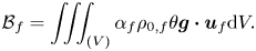 \begin{equation} \mathcal{B}_{f}= \iiint_{(V)}\alpha_{f}\rho_{0,f}\theta \boldsymbol{g}\boldsymbol{\cdot} \boldsymbol{u}_f\mathrm{d}V. \end{equation}
Combining (2.12) with (7.1) leads to
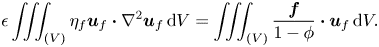 \begin{equation} \epsilon \iiint_{(V)}\eta_{f} \boldsymbol{u}_{f}\boldsymbol{\cdot}\nabla^{2}\boldsymbol{u}_{f}\, \mathrm{d}V = \iiint_{(V)}\frac{\boldsymbol{f}}{1-\phi} \boldsymbol{\cdot} \boldsymbol{u}_{f}\, \mathrm{d}V. \end{equation}
This relation links quantitatively the efficiency parameter to the coupling force between the fluid and particles. In our case, for laminar convection, the coupling force (2.14) can be used and we obtain
 \begin{equation} \iiint_{(V)}\boldsymbol{f}\boldsymbol{\cdot} \boldsymbol{u}_{f}\, \mathrm{d}V=\iiint_{(V)}\beta \frac{\eta_{f}}{r^{2}}(\boldsymbol{u}_{f}-\boldsymbol{u}_{p})\boldsymbol{\cdot} \boldsymbol{u}_{f}\, \mathrm{d}V. \end{equation}
As discussed earlier, as  $St\ll 1$, particles are statistically passive tracers. Nevertheless, we observed experimentally the formation of cumulates, so there is a weak component of particle motion that enables settling. In this way, we assume the following decomposition for the particle velocity:
 \begin{equation} \boldsymbol{u}_{p}=\boldsymbol{u}_{f}+\boldsymbol{u}_{s}, \end{equation}
where  $\boldsymbol {u}_{s}$ stands for the settling velocity, which is considered to be the Stokes velocity, and verifies
  $\| \boldsymbol {u}_{f}\| \gg \| \boldsymbol {u}_{s}\|$ in our case. This hypothesis is also corroborated by the experiments done by Lavorel & Le Bars (Reference Lavorel and Le Bars2009), who showed that particles in turbulent convection settle at a speed that scales with the Stokes velocity. Equation (7.4) thus suggest the (order-of-magnitude) balance
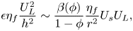 \begin{equation} \epsilon \eta_{f} \frac{U_{L}^{2}}{h^{2}}\sim \frac{\beta(\phi)}{1-\phi} \frac{\eta_{f}}{r^{2}}U_{s}U_{L}, \end{equation}
where the convective velocity scales are 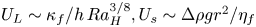 $U_{L}\sim \kappa _{f}/h\, Ra_{H}^{3/8}, U_{s}\sim \Delta \rho g r^{2}/\eta _{f}$ and where
  $\beta (\phi )/(1-\phi )\approx 0.5-1$ in our experiments, which yields
 \begin{equation} \epsilon\sim \frac{h^{2}}{r^{2}}\frac{U_{s}}{U_{L}}\sim \frac{\overline{\Delta \rho} g h^{3}}{\eta_{f} \kappa_{f} } \, Ra_{H}^{{-}3/8}, \end{equation}
which relates the efficiency parameter to the physical properties of the fluid and particles.
To verify this expression in our experiments, we rewrite (5.3) by substituting  $\epsilon$ with (7.7) and deduce a new scaling law for the maximal concentration of particles in the suspension
 \begin{equation} \phi_{{max}}\sim \frac{h}{r} \bar \zeta. \end{equation}
As a consequence, the proxy  $\varphi$ of the particle concentration should also follow this law
  $\varphi =C_{\varphi } h/r \bar \zeta$, with
  $C_{\varphi }$ a constant that is constrained experimentally
  $C_{\varphi }=8.10^{-4}$ (figure 13).

Figure 13. Proxy of particle concentration at steady state for all experiments where particles in suspension are heavier than the fluid. The blue dashed line stands for the transition between the cumulate regime, and the absolute suspension one, using our model based on (7.8).
To verify qualitatively the consistency of this expression with  $\epsilon$, we compare (5.3) and (7.8) to get an expression for the efficient coefficient
 \begin{equation} \epsilon=\frac{C_{\varphi}a}{C_{s}} \frac{\overline{\Delta \rho} g h^{3}}{\eta_{f} \kappa_{f} } \, Ra_{H}^{{-}3/8}. \end{equation}
Assuming that particles are packed randomly in the floating lid ( $a=0.56$), we get the average value of
  $\epsilon = 4\pm 3\,\%$ in our experiments. This estimate is slightly higher than the values reported in the literature but still consistent with them (Solomatov et al. Reference Solomatov, Olson and Stevenson1993; Lavorel & Le Bars Reference Lavorel and Le Bars2009). However, the main purpose of this physical argument is to show how to reconcile Solomatov's ad hoc expression with the complete physical framework that governs the two-phase flow and to verify it qualitatively. Experiments where the bulk concentration of beads is precisely measured are required to corroborate quantitatively this reasoning.
7.3. Application to magma oceans
7.3.1. Crystal segregation in magma ocean
Based on the model developed above, we propose an insight into the segregation process of particles in the thermal history of a magma ocean, and especially the flotation of plagioclase. This type of crystal is known to be lighter than the residual liquid from which they form (Elkins-Tanton et al. Reference Elkins-Tanton, Burgess and Yin2011). The flotation of plagioclase is the main scenario invoked to explain the formation of the light anorthosite crust of the Moon (Wood Reference Wood1970; Solomon & Longhi Reference Solomon and Longhi1977). Convection driven by secular cooling is the relevant regime for convective magma ocean. Secular cooling is mathematically equivalent to internal heating treated in our model (see, e.g. Krishnamurti Reference Krishnamurti1968).
Deschamps et al. (Reference Deschamps, Yao, Tackley and Sanchez-Valle2012) demonstrated that scaling laws that describe thermal convection in volumetrically heated Cartesian boxes are also valid in a spherical geometry, provided we take into account a geometrical factor describing the shell curvature. In this case, the surface heat flux is linked to the secular cooling and the internal heating rate as follows:
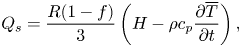 \begin{equation} Q_{s}=\frac{R(1-f)}{3}\left(H-\rho c_{p} \frac{\partial \overline{T}}{\partial t}\right), \end{equation}
where  $f=(R-h)/R$ is the ratio between the depth of the magma ocean
  $h$ and the planetary radius
  $R$. Further details can be found in Appendix B.
The value of  $Q_{s}$ ranges from
  $10^{6}\ \mathrm {W\ m}^{-2}$ for molten planetary bodies that release heat by radiation to space (Elkins-Tanton et al. Reference Elkins-Tanton, Burgess and Yin2011; Massol et al. Reference Massol2016), down to
  $10^{-3}-10^{-2}\ \mathrm {W\ m}^{-2}$ when the flotation crust is present (Maurice et al. Reference Maurice, Tosi, Schwinger, Breuer and Kleine2020). All physical quantities used in the model are summarized in table 5.
Table 5. Physical parameters used in the model.
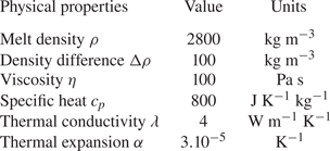
We deduce the critical particle radius enabling crystal flotation for two types of magma ocean: a 200 km deep shallow lunar magma ocean ( $R=1737\ \mathrm {km}, f=0.88, g=1.6\ \mathrm {m\ s}^{-2}$) and a fully molten planetesimal (
 $R=300\ \mathrm {km}, f=0.42, g=0.23\ \mathrm {m\ s}^{-2}$). This critical radius
  $r_c$ is calculated from the critical Shields number (4.13)
 \begin{equation} r_c=\frac{\kappa \eta}{h\Delta \rho g \zeta_c} \left(\frac{\alpha \rho g Q_s h^4}{\eta \kappa \lambda}\right)^{3/8}. \end{equation}
Results are displayed in figure 14. As the crystal size during crystallization is estimated to be in the range  $r=0.1\text {--}10\ \mathrm {mm}$ (Solomatov Reference Solomatov2000), we deduce that crystals float during magma ocean cooling. Magma ocean episodes enable efficient crystal segregation. This segregation is less efficient for smaller bodies such as planetesimals (with
  $R\le 300\ \mathrm {km}$), suggesting that the crystallization history might be more complex in these cases. We compared our results with those displayed in Elkins-Tanton (Reference Elkins-Tanton2012) based on the law of Solomatov et al. (Reference Solomatov, Olson and Stevenson1993)
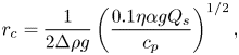 \begin{equation} r_c=\frac{1}{2\Delta \rho g} \left(\frac{0.1 \eta \alpha g Q_s}{c_p}\right)^{1/2}, \end{equation}
with  $\eta =0.1\ \mathrm {Pa\ s}$. Equation (7.12) was considered by these authors to be applicable in both laminar and turbulent experiments but established for a system heated from below. Here, we propose a model for convective systems driven by secular cooling. Our model enables smaller particles to participate in crust formation.
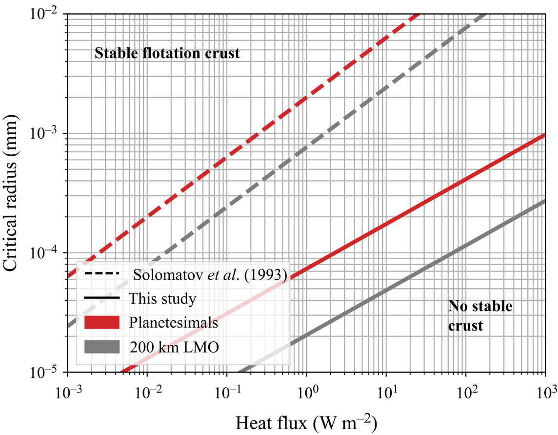
Figure 14. Diagram of flotation vs suspension for two planetary bodies. Each solid line corresponds to the critical radius  $r_c$ given by (7.11). Particles with radius greater than the critical one are allowed to float, otherwise they stay in suspension. Dashed line shows the critical radius of crystals predicted by Solomatov's law (7.12).
7.3.2. Crust thickness and flotation efficiency
Our model not only provides criteria for the formation of stable crystal reservoirs, floating crust or cumulates, but can also be used to quantify the partitioning of the crystals between the suspension and these deposits. We illustrate how to quantify this partition of crystals between the deposits and the convective bulk in the particular case of the lunar magma ocean (LMO).
In the literature, it is widely assumed that all plagioclase crystals settle instantaneously once they nucleate in the LMO (Elkins-Tanton et al. Reference Elkins-Tanton, Burgess and Yin2011; Maurice et al. Reference Maurice, Tosi, Schwinger, Breuer and Kleine2020), which yields a system composed of a flotation crust growing above a purely liquid magma ocean. The main results of these two studies are indicated by the two highlighted bands in figure 15. This hypothesis was relaxed using the flotation efficiency, which is the ratio between the volume of crystals that float and the total volume of crystals that nucleate in the system. This parameter can be estimated from field data. For instance, Namur et al. (Reference Namur, Charlier, Pirard, Hermann, Liégeois and Auwera2011) determined the value for plagioclase flotation by studying the Sept Iles layered intrusion, and they found an efficiency of 50 %. They assumed that this flotation efficiency would be the same in the case of the LMO, and they use it to constrain the amount of plagioclase that composed the anorthosite crust and its thickness. Charlier et al. (Reference Charlier, Grove, Namur and Holtz2018) used the crustal thickness measured by spacecraft gravity data (Wieczorek et al. Reference Wieczorek2012) and a flotation efficiency in the range between 40 % and 100 % in order to constrain the thickness of the LMO.
Figure 15. Evolution of the maximal thickness of the anorthosite crust formed by plagioclase flotation above the lunar magma ocean as a function of the crystal size and the surface heat flux. We represent also the range of surface heat flux that is simulated by two thermal models (Elkins-Tanton et al. Reference Elkins-Tanton, Burgess and Yin2011; Maurice et al. Reference Maurice, Tosi, Schwinger, Breuer and Kleine2020).
This ad hoc parameter can be discussed in the light of our model. According to the present study, if the initial volume of crystals is smaller than the critical volume that can be sustained at the surface, all crystals form a flotation crust. If the crust has reached its maximum thickness, the crystals ‘in excess’, i.e. that cannot be incorporated in the crust, remain in suspension. This is a fundamentally different way of thinking which links crystal flotation to physical parameters.
We consider that the LMO is a shallow shell corresponding to 20 vol% of the total volume of the Moon. This high level of solidification is necessary to trigger plagioclase crystallization (Elkins-Tanton et al. Reference Elkins-Tanton, Burgess and Yin2011). The evolution of the maximal thickness sustainable at the surface of the LMO is displayed in figure 15. The crystal size has almost no influence on the steady state crustal thickness except at the low limit. This is due to the sub-critical value of the Shields number, which is essentially constrained by the low value of the melt viscosity. In order to form a crust with a thickness of 40 km corresponding to current estimates of the lunar crust, our model predicts that the surface heat flux should be below  $3\ \mathrm {W\ m}^{-2}$. In the cases of Elkins-Tanton et al. (Reference Elkins-Tanton, Burgess and Yin2011) and Maurice et al. (Reference Maurice, Tosi, Schwinger, Breuer and Kleine2020), 100 % flotation efficiency would imply a thicker crust. Our model adds some physical constraints on the LMO evolution in general, by coupling quantitatively the segregation of crystals to the thermal history.
We emphasize that our reasoning is dealing with the stability of the crust and its steady state. The predicted crust thickness is reached after a time-dependent deposition process which is not discussed in this paper. It requires a complete description of the transient regime of the flotation crust.
7.3.3. Limitation of the model
We aim to illustrate how the criteria developed in this paper can be applied to natural systems and how they can provide new constraints on conditions under which a deposit can form or not. Of course, our illustration is a crude approximation of the complexity of the magma ocean. We use simplified hypotheses, but the framework we propose here is robust enough to enable refinements that can be added at will in order to include complexity.
Our first strong assumption is the bulk crystallization that was abundantly considered in the literature as a common end member (Solomatov Reference Solomatov2000; Elkins-Tanton et al. Reference Elkins-Tanton, Burgess and Yin2011). This is justified by the nature of convection driven by secular cooling, which implies that crystals nucleate within the cold downwellings that end up in an isentropic convective bulk. For small-size bodies, this is equivalent to an isothermal interior.
We also assume that crystals are non-cohesive, as in experiments. This hypothesis is compatible with batch crystallization where crystals nucleate in the convective bulk. This regime of crystallization is consistent with magma oceans, but may not be for smaller magmatic reservoirs such as magma chambers or lava lakes. In these cases, crystals may mainly form at the boundary of the system, directly where they are supposed to settle. This adds a complexity to the system as cohesion between crystals becomes important. One way to take cohesion into account in the present model may be by increasing the erosion threshold  $\zeta _c$. The stronger the interactions between crystals are, the higher the value of
  $\zeta _c$.
In addition, we did not consider in detail the effect of crystallization series on the evolution of composition and its consequences on all the physical parameters such as the number of crystals, crystal size and liquidus and solidus temperatures. We expect that in the limit of small crystal fractions, our results would still apply, but the transient behaviour of crystallizing systems needs to be studied specifically.
Moreover, our model does not take into account the influence of pressure on all the physical parameters. This hypothesis is consistent with small planetary bodies such as planetesimals, or with the latest stages of shallow magma oceans, but it is less justified for larger bodies such as the Earth. In the latter case, pressure would affect the whole thermodynamics, as it influences the geotherm, the solidus and liquidus of crystals, the viscosity of the liquid magma, the formation of crystals, etc. In these cases, our stability criterion based on the Shields number is still valid, but the threshold value and the scaling laws that are involved should be adapted accordingly.
Furthermore, we described the system by adopting a stability criterion as did Solomatov. But magma oceans are evolving systems where temperature varies a lot during the thermal history. Hence, describing their complex behaviour over time thanks to a stationary criterion is a strong assumption that has to be relaxed. Complete thermal model that takes into account the kinetics of sedimentation and erosion is required to deal with suspension stability in magma oceans. Erosion/deposition mechanisms commonly used in geomorphology (Charru et al. Reference Charru, Mouilleron and Eiff2004; Lajeunesse et al. Reference Lajeunesse, Malverti and Charru2010) could be further revisited in terms of crystal erosion and sedimentation in magmatic reservoirs.
We considered here the high Prandtl limit where inertia is negligible compared with viscous forces. Nonetheless, magma oceans have experienced turbulent episodes (Solomatov Reference Solomatov2000) that imply high Rayleigh numbers that are not yet attainable experimentally or numerically. This seems to be all the more true for large bodies. In this case, scaling laws used for the thermal state have to be adapted. For instance, Kraichnan (Reference Kraichnan1962) expressed the different scaling law for turbulent flow, depending on the Prandtl number. It would lead to other scaling laws for the shear stress and thus other expressions for the Shields number. But fundamentally, the bases of our approach would remain true even in the turbulent case.
8. Conclusion
Particles sheared in a convective fluid can form deposits, floating crusts or cumulates, depending on the sign of their buoyancy. Using laboratory experiments, we proposed a model that estimates the partitioning of particles in such systems at high Prandtl number and for Rayleigh–Roberts numbers up to  $10^{9}$. Our model is based on the estimation of one dimensionless parameter that encapsulates the main physical ingredients required to describe the system: the generalized Shields number
  $\zeta$ that compares the buoyancy of particles with the shear stress generated by convection. The value of this parameter quantifies both the thickness of the flotation crust, and the maximal concentration of crystals that can be sustained in suspension. The volume of particles that forms a cumulate can be deduced from these two pieces of information by a mass budget. This unifying framework can be adapted to understand transient episodes of the thermal history of natural systems driven by secular cooling and/or internal heating. In order to do so we need to complete the model by the detailed description of the dynamics of erosion and deposition, and in particular of the characteristic time scales that are involved. These time scales have to be compared with the convective system cooling time scale. Further studies are needed to completely understand the feedback existing between these intricate time scales. This is a necessary step in order to explain the wealth of the observed structures in planetary bodies and in their vestiges that reach us as meteorites.
Supplementary material
Supplementary material are available at https://doi.org/10.1017/jfm.2021.862.
Acknowledgements
This paper is part of C. Sturtz's PhD thesis (Université de Paris, Institut de Physique du Globe de Paris). The authors thank Pr. Chomaz and two anonymous reviewers for their fruitful comments that improved the paper. This study contributes to the IdEx Université de Paris ANR-18-IDEX-0001.
Funding
This work was supported by the Programme National de Planétologie (PNP) of CNRS/INSU, co-funded by CNES, and by the ANR V-Care-18-CE03-0010.
Declaration of interest
The authors report no conflict of interest.
Appendix A. Reynolds numbers and DBL
With rigid boundary condition, one can define the DBL as the region where the velocity tends to zero. The thickness of the DBL can be expressed from the balance between the convective term and the diffusion term in the conservation of momentum equation (e.g. Jaupart & Mareschal Reference Jaupart and Mareschal2010, p. 128)
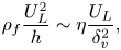 \begin{equation} \rho_{f}\frac{U_{L}^{2}}{h}\sim \eta \frac{U_{L}}{\delta_{v}^{2}}, \end{equation}
which leads to 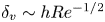 $\delta _{v}\sim h Re^{-1/2}$, where
 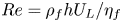 $Re=\rho _{f}hU_{L}/\eta _{f}$ is the Reynolds number. This relation justifies quantitatively that the DBL occupies the entire reservoir in the laminar limit, which is the regime reached in our experiments (figure 16).

Figure 16. Scaling laws for the horizontal (a) and vertical (b) Reynolds numbers in internally heated convective systems.
The scaling law that characterizes velocity in internally heated convective systems can be rewritten in terms of Reynolds number  $Re$ using (4.11)
 \begin{equation} Re\sim Ra_{H}^{3/8} Pr^{{-}1}, \end{equation}
which has been verified experimentally as illustrated in figure 16. The pre-factors for the horizontal and vertical Reynolds numbers are given in table 6.
Table 6. Parameters of power laws determined experimentally for the vertical and horizontal Reynolds numbers.

Appendix B. Secular cooling and internal heating
In geophysical systems evolving over long periods of time, the thermal state is transient, so one can argue that our reasoning is not applicable as scaling laws that are used here hold only at steady state. Here, we will show that it is possible to adapt them to describe the transient state.
First, we treat the floating lid as a homogeneous layer where Fourier's law can be applied. In the transient state, the heat flux departs from (4.1), which is valid only in steady state conditions. Hence, we can define the diffusive time scale in the floating lid  $\tau _{{diff}}=\delta ^{2}/\bar \kappa$, with
  $\bar \kappa =\bar \lambda / \bar \rho \, \bar c_{p}$ the thermal diffusivity of the floating lid where
  $\bar \lambda, \bar \rho$ and
  $\bar c_{p}$ are respectively its average thermal conductivity, density and specific heat. This time scale is compared with the time scale related to the evolution of the thermal state of a convective fluid heated from inside. The latter is given by
 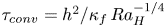 $\tau _{{conv}}=h^{2}/\kappa _{f}\, Ra_H^{-1/4}$ (Limare et al. Reference Limare, Jaupart, Kaminski, Fourel and Farnetani2019). Thus, the criterion that ensures that the lid's thermal state evolves quasi-statically is based on the ratio
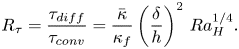 \begin{equation} R_{\tau}=\frac{\tau_{{diff}}}{\tau_{{conv}}}=\frac{\bar \kappa}{\kappa_{f}} \left(\frac{\delta}{h}\right)^{2} \, Ra_{H}^{1/4}.\end{equation}
If  $R_{\tau }\ll 1$, the lid reaches its steady state quickly and (4.1) holds true. In our experiments,
  $R_{\tau }\approx 0.1\text {--}0.5$, so the approximation is justified. In geophysical systems, the approximation holds true if
  $Ra_{H}$ is moderate and/or if the floating lid is thin compared with the depth of the convective mantle. For instance, for lids that represent
  $\delta /R=1\,\%$ equivalent to the ratio between the lithosphere thickness and the Earth's radius, the quasi-static approximation is correct for
  $Ra_{H}$ up to
  $10^{12}$, which is relevant for geophysical applications.
Second, the model is based on scaling laws that describe the thermal state of convective systems heated internally. In the transient state, the secular cooling term can be considered as an additional source of internal heat. We define the modified rate of internal heat generation as
 \begin{equation} H^{*}=H-\rho_{f} c_{p,f}\frac{\partial \overline{T}}{\partial t}. \end{equation}
In this way, the Rayleigh–Roberts number is also modified
 \begin{equation} Ra_{H}^{*}=\frac{\alpha_{f} \rho_{0,f} g H^{*}h^{5}}{\eta_{f} \kappa_{f} \lambda_{f}}. \end{equation}
Thus, the drop of temperature across the TBL becomes
 \begin{equation} \Delta T_{TBL}=C_{T}^{*} \frac{H^{*}h^{2}}{\lambda_{f}} (Ra_{H}^{*})^{{-}1/4}. \end{equation}
Limare et al. (Reference Limare, Kenda, Kaminski, Surducan, Surducan and Neamtu2021) showed that this model describes well the transient state in experimental convective systems. The authors measured  $C_{T}^{*}=3.58 \pm 0.15$ similar to the value retrieved from experiments in homogeneous, steady state conditions. This model was further used to describe the thermal evolution of parent bodies of iron meteorites (Kaminski et al. Reference Kaminski, Limare, Kenda and Chaussidon2020). It shows that convective systems where convection is mainly driven by secular cooling can also be treated in the framework presented in this paper.
Consequently, we are able to estimate the evolution of the Shields number from the thermal history of such systems, enabling the study of the formation of floating crust and/or deposits.


 Open access