




1 Introduction
The interaction of fluids with structures has long attracted the attention of scientists due to its importance in the design of products in many traditional engineering fields such as aeronautics, wind engineering and off-shore oil extraction. The divergence and flutter analysis of wings is for instance an important step in the design of an aircraft, since these phenomena may induce premature fatigue and even lead to fracture of the structure. The vortex-induced vibration of elongated marine risers is another example of an industrial system where structural oscillations are detrimental. Because of the high flow speeds and the large scales of the structures encountered in most of these applications, inviscid models have often been used to describe the high Reynolds number flows (Dowell Reference Dowell2004).
However, neglecting the viscous effects in the aerodynamic model is not always possible, for instance when addressing the aeroelastic design of micro- and unmanned air vehicles that fly at lower speed. New phenomena may occur, such as the spontaneous pitching oscillations of airfoils, observed and characterized experimentally by Poirel, Harris & Benaissa (Reference Poirel, Harris and Benaissa2008) for the transitional flow regime ( $Re=10^{4}{-}10^{5}$). The use of a viscous flow model is then essential to capture the laminar flow separation at the origin of the airfoil oscillations. In the renewable energy industry, new concepts are developed to exploit the flow-induced vibrations of small-scale structures (Young, Lai & Platzer Reference Young, Lai and Platzer2014) and transform their kinetic energy into energy using piezoelectric and electromagnetic technologies (Khaligh, Zeng & Zheng Reference Khaligh, Zeng and Zheng2009). For instance, Leontini & Thompson (Reference Leontini and Thompson2012) showed that a small active rotational oscillation of an elastically mounted cylinder can result in very large transverse oscillations, and is therefore an efficient method to transfer energy from the fluid to the structure. Peng & Zhu (Reference Peng and Zhu2009) proposed a purely passive device relying on self-induced and self-sustained oscillations. Rather than actively controlling the pitching motion, the foil motion is completely excited by flow-induced instability, using the same mechanism responsible for flutter of airfoils. Recent advances in energy harvesting from flow-induced vibrations or aeroelastic phenomena can be found in the review by Abdelkefi (Reference Abdelkefi2016). The main aim when designing an energy harvesting system is to predict the geometrical and physical properties of the system allowing sustained oscillating limit cycles to emerge (Olivieri et al. Reference Olivieri, Boccalero, Mazzino and Boragno2017). The simple argument to identify such oscillating states is based on a simple resonance condition between the natural frequencies of the flow and structure. But the validity of this resonance condition strongly depends on the solid-to-fluid density ratio. For density ratios close to unity, typical of fluid–structure experiments in water experimental facilities, large-amplitude oscillations can be obtained even far from the resonance condition (see for instance Mittal (Reference Mittal2016) for the vortex-induced vibration of a circular cylinder). Numerical simulations of the evolution equations governing the coupled fluid–solid nonlinear dynamics can be performed to explore the existence of self-sustained oscillating states and to characterize the vibration amplitude that results from the nonlinear saturation. However, the complex dynamics obtained with those temporal simulations is somehow difficult to analyse and the inherent nonlinearity of this approach prevents us from identifying simple linear mechanisms that may be predominant, and explaining the emergence of self-sustained oscillations. One of the objectives of the present study is to use linear stability analyses of the coupled fluid–structure problem so as to predict regions of the parameter space where self-sustained fluid–solid oscillations occur and to characterize their frequency. Such linear analyses have successfully been used to predict and explain the vortex-induced vibrations of rigid bodies (Mittal Reference Mittal2016) or the wake-induced oscillatory paths of rigid bodies freely rising or falling in fluids (Tchoufag, Fabre & Magnaudet Reference Tchoufag, Fabre and Magnaudet2014a; Tchoufag, Magnaudet & Fabre Reference Tchoufag, Magnaudet and Fabre2014b). In the same spirit, we aim here at simulating the self-sustained deformation of elastic splitter plates attached to the rear of a circular cylinder immersed in an incompressible flow and explaining the emergence of those limit cycle solutions based on a linear stability analysis. In the following subsections, we review previous studies, first on the flow past a circular cylinder with rigid and flexible splitter plates, and then on the linear fluid–solid stability analyses of rigid and flexible structures interacting with wake flows.
1.1 Interaction of the circular cylinder wake flow with rigid and flexible splitter plates
Among passive control methods, a rigid splitter plate has been one of the most successful devices to control the vortex shedding behind bluff bodies. The control of the turbulent vortex shedding was experimentally investigated first by Roshko (Reference Roshko1954) and Roshko (Reference Roshko1955) for a circular cylinder at Reynolds number  $Re=5000$ (based on the cylinder diameter $D^{\ast }$ and the uniform inflow velocity $U_{\infty }^{\ast }$) and then by Bearman (Reference Bearman1965) for other bluff body wake flows. For higher Reynolds number flows ( $10\,000<Re<50\,000$), Apelt, West & Szewczyk (Reference Apelt, West and Szewczyk1973) observed that splitter plates have an effect of increasing the base pressure and thus significantly reducing the drag. For lower Reynolds number flows ( $140<Re<3600$), Unal & Rockwell (Reference Unal and Rockwell1988) showed that splitter plates reduce the absolute instability responsible for the onset of vortex shedding. Numerical simulations of the two-dimensional incompressible Navier–Stokes equations were performed by Kwon & Choi (Reference Kwon and Choi1996) in the range of lower Reynolds numbers $80<Re<160$. The vortex shedding completely disappears when the length of the splitter plate is larger than a critical length that is proportional to the Reynolds number. Mittal (Reference Mittal2003) investigated the effect of a ‘slip’ splitter plate, to further understand the control mechanism at play. Other configurations of splitter plates have been considered, such as for instance two splitter plates symmetrically arranged (Bao & Tao Reference Bao and Tao2013).
When the rigid splitter plate is attached to a circular cylinder that is now free to rotate around its axis, a striking symmetry breaking of the configuration may appear depending on the length  $L^{\ast }$ of splitter plate. The cylinder and splitter plate then migrate to a asymmetric equilibrium position, for which the moment exerted by the fluid forces is equal to zero. Such symmetry breaking was first observed experimentally by Cimbala, Garg & Park (Reference Cimbala, Garg and Park1988), Cimbala & Garg (Reference Cimbala and Garg1991) and Cimbala & Chen (Reference Cimbala and Chen1994) for large Reynolds number flows, and more recently by Gu et al. (Reference Gu, Wang, Qiao and Huang2012). At lower Reynolds numbers ( $Re<100$), two-dimensional numerical simulations of the flow in conjunction with the rotational dynamics of the body were performed by Xu, Sen & Gad-el Hak (Reference Xu, Sen and Gad-el Hak1990) for plate lengths in the range $0.5<L^{\ast }/D^{\ast }<2$. The symmetry-breaking bifurcation appears when increasing the Reynolds number above a critical value that depends on the ratio between the plate length and cylinder diameter $L^{\ast }/D^{\ast }$. Further increasing the Reynolds number, Xu, Sen & Gad-el Hak (Reference Xu, Sen and Gad-el Hak1993) identified a supercritical Hopf bifurcation leading to the oscillation of the splitter plate around a asymmetric position. The effect of adding a restoring and dissipative moment at the elastic centre was recently investigated by Lu et al. (Reference Lu, Guo, Tang, Liu, Chen and Xie2016) for the low Reynolds number of $Re=100$. For the same Reynolds number, a similar symmetry-breaking bifurcation was reported by Bagheri, Mazzino & Bottaro (Reference Bagheri, Mazzino and Bottaro2012) for a flexible filament hinged to a circular cylinder. This is a flexible splitter plate with infinitesimally small thickness $H^{\ast }$, which is allowed to rotate about the hinge point at the base of the cylinder. They reported spontaneous deviations for splitter plates of length $L^{\ast }<2D^{\ast }$, as for the rotatable rigid splitter plate (Xu et al. Reference Xu, Sen and Gad-el Hak1990). A semi-empirical model has been later proposed by Lacis et al. (Reference Lacis, Brosse, Ingremeau, Mazzino, Lundell, Kellay and Bagheri2014) to predict the deviation and an analogy with an inverse pendulum was proposed to explain the occurrence of this phenomenon.
The dynamics of flexible splitter plates, free to continuously deform along their length due to the fluid forces acting on them, was recently investigated experimentally by Shukla, Govardhan & Arakeri (Reference Shukla, Govardhan and Arakeri2013). For a plate of length  $L^{\ast }=5D^{\ast }$, they identified several regimes of splitter plate motions when varying the Reynolds number in the range $1800<Re<10^{4}$. Two regimes of periodic motions, characterized by a non-dimensional frequency $f^{\ast }D^{\ast }/U_{\infty }^{\ast }\sim 0.15{-}0.2$, were found for low and high Reynolds numbers, and separated by a regime of aperiodic motion. The magnitude of the tip displacement was also found to vary strongly and non-monotonically, especially for the lower values of bending stiffness explored in that study. Meanwhile, Lee & You (Reference Lee and You2013) performed numerical simulations for the low Reynolds number of $Re=100$ while varying the plate’s length and stiffness. For smaller plate lengths, they obtained a non-monotonic variation of the frequency and magnitude of the tip displacement when varying the bending stiffness. In addition, the splitter plate was found to vibrate like a first- (respectively second) bending mode for $L^{\ast }=D^{\ast }$ (respectively $L^{\ast }=2D^{\ast }$). For the larger plate’s length $L^{\ast }=3D^{\ast }$, a monotonic variation of the oscillating frequency and magnitude of the tip displacement is reported, and the vibration shape of the splitter plate was a combination of the first- and second-bending mode. Wu, Qiu & Zhao (Reference Wu, Qiu and Zhao2014) investigated the control of the vortex shedding past a circular cylinder at $Re=150$ by using an attached flexible filament of length $D^{\ast }<L^{\ast }<3D^{\ast }$. By varying the flexibility of the filament stiffness, they concluded that the fluctuation of lift force and vortex shedding of a fixed cylinder can be suppressed efficiently. Using a viscoelastic model of the splitter plate attached to the circular cylinder immersed in a channel flow, Mishra et al. (Reference Mishra, Kulkarni, Bhardwaj and Thompson2019) concluded that a careful tuning of the damping may be effectively employed, to suppress flow-induced vibration when it is detrimental to the structure, or to enhance power output for energy extraction applications.
If unsteady simulations give the amplitude and frequency of the self-sustained oscillations resulting from the interaction of the flexible splitter plate with the flow, they provide only a limited overview of the underlying destabilizing linear mechanisms at play. For instance, Lee & You (Reference Lee and You2013) concluded that the Strouhal number of vortex shedding or the frequency of plate deflection were difficult to estimate using natural frequencies of the plate’s bending modes. It is therefore unclear whether a resonance condition between the frequency of the hydrodynamic vortex-shedding mode and that of the plate’s bending modes may apply. Moreover, to our knowledge, a global stability analysis of the fluid–structure interaction has never been performed to explain the symmetry breaking of the flexible splitter plate configuration. In the present study, we thus propose to use linear fluid–solid stability analyses so as to better identify and characterize the various regimes of interaction of the splitter plate with the wake flow.
1.2 Linear stability analysis for fluid–rigid and fluid–elastic interactions
Using linear analysis to unravel the mechanism at play in the fluid–structure interaction is not new. Classical aeroelasticity is mainly based on linear analysis, and the flutter and divergence instability of wings can be predicted by considering a linear model of the interaction between the fluid and the solid (Bisplinghoff, Ashley & Halfman Reference Bisplinghoff, Ashley and Halfman1955). The fluid–structure stability analysis refers here to an investigation of the temporal evolution of infinitesimally small perturbations than develop in a time-independent solution of the fluid–structure interaction problem. Conceptually, this is very similar to hydrodynamic stability analysis, but the time-independent solution as well as the temporal perturbations may be both in the flow and the structure. The additional theoretical and numerical difficulty in performing stability analyses in fluid–structure interaction problems is taking into account rigorously the perturbation of the fluid–solid interface motion. Linear stability analysis has been predominantly applied to fluid–solid configurations where the solid is rigid and its dynamics is described by few degrees of freedom. For instance, the transverse displacement of a spring-mounted cylinder facing a uniform flow is simply governed by a damped harmonic oscillator. In most of the following studies, the flow equations can then be rewritten in a frame of reference attached to the rigid solid. To our knowledge, the first linear stability analysis of a spring-mounted rigid body was performed by Cossu & Morino (Reference Cossu and Morino2000) to investigate the vortex-induced vibration of a circular cylinder in a laminar flow regime. They found the existence an unstable fluid–solid eigenmode for sub-critical values of the Reynolds number, i.e. below the critical value given by a purely hydrodynamic stability analysis (Zebib Reference Zebib1987). For these sub-critical Reynolds numbers, Mittal & Singh (Reference Mittal and Singh2005) then showed that results of the linear stability analysis are in good agreement with those of two-dimensional direct numerical simulations. The mechanism of frequency lock-in of the fluid–structure to the natural frequency of the solid (the frequency of the spring in vacuum) was later on investigated with linear stability analysis by Mittal (Reference Mittal2016) for the spring-mounted circular-cylinder flow in a laminar subsonic flow regime, and by Gao, Zhang & Ye (Reference Gao, Zhang and Ye2016), Gao et al. (Reference Gao, Zhang, Li, Liu, Quan, Ye and Jiang2017) for a spring-mounted airfoil in turbulent transonic buffeting flow. The wake-induced oscillatory paths of bodies freely rising or falling in fluids (see Ern et al. (Reference Ern, Risso, Fabre and Magnaudet2012) for a review) have also been investigated using fluid–solid stability analysis. They revealed the essential role of the wake in the path instability of buoyancy-driven disks/thin cylinders (Tchoufag et al. Reference Tchoufag, Fabre and Magnaudet2014a) and of freely rising spheroidal bubble (Tchoufag et al. Reference Tchoufag, Magnaudet and Fabre2014b). Fewer authors have investigated the linear stability of fully deformable structures in flows. The flutter instability of a thin flexible plate in channel flow was first investigated by Shoele & Mittal (Reference Shoele and Mittal2016) using an inviscid flow model, and then by Cisonni et al. (Reference Cisonni, Lucey, Elliott and Heil2017) using a viscous flow model and time-marching simulations. The effect of structural inhomogeneity on the flutter instability of elastic cantilevers was further investigated by Cisonni, Lucey & Elliott (Reference Cisonni, Lucey and Elliott2019). A linear and nonlinear analysis of the dynamics of an inverted-flap flapping in a low Reynolds number flow was also performed by Goza, Colonius & Sader (Reference Goza, Colonius and Sader2018). The effect of a compliant wall on the growth of perturbations developing in a Blasius boundary layer was considered investigated by Tsigklifis & Lucey (Reference Tsigklifis and Lucey2017) with modal and non-modal linear stability analyses of the fluid–structure interaction. In all of these studies, the elastic thin structure was modelled with a one-dimensional elastic beam. The more general case of a finite-thickness structure modelled with the nonlinear Saint Venant–Kirchoff constitutive relation was recently considered by Pfister, Marquet & Carini (Reference Pfister, Marquet and Carini2019) for some of the fluid–solid configurations previously mentioned. The linear stability analysis then relies on a linearization of the nonlinear equations governing the incompressible flow and the elastic structure that are coupled using the arbitrary Lagrangian Eulerian (ALE) method. This approach, that we will follow, has the advantage of preserving a high-quality description of the fluid–solid conform interface, at the price of introducing an arbitrary extension operator for propagating the solid interface deformations onto the fluid domain.
The paper is organized as follows. In § 2, we present first the governing parameters of this fluid–solid configuration and then the mathematical formulation of the fluid–solid interaction. The nonlinear governing equations are briefly introduced before describing the fully coupled as well as the simplified quiescent-fluid and quasi-static linear stability analyses. Simulation results of the unsteady nonlinear dynamics are presented in § 3, where several regimes of interaction, identified when decreasing the plate’s stiffness, are carefully described. Results of various linear stability analyses are finally presented in § 4 so as to better characterize the linear mechanisms at play in the emergence of these nonlinear regimes.
2 Fluid structure configuration and formulations
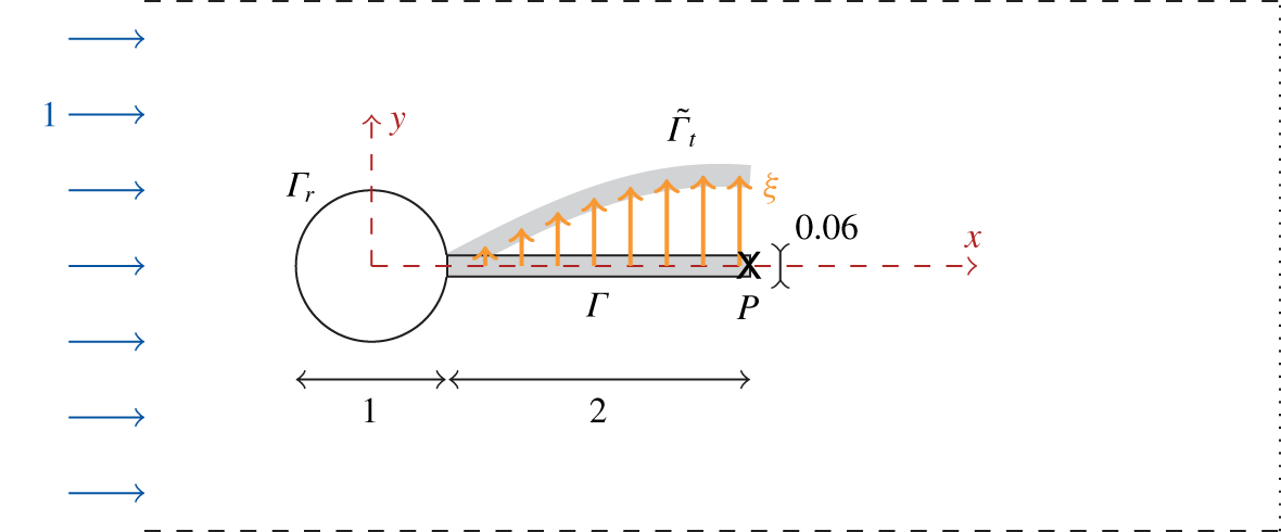
Figure 1. Sketch of the elastic plate (grey, boundary  $\unicode[STIX]{x1D6E4}$ in the reference configuration and $\tilde{\unicode[STIX]{x1D6E4}}_{t}$ in the deformed configuration) clamped on the rigid cylinder (white, boundary $\unicode[STIX]{x1D6E4}_{r}$) and immersed in a uniform incoming flow field (blue arrows). Lengths/velocity are made non-dimensional using the inlet velocity and the cylinder’s diameter. The plate’s tip is marked by the point $P(2.5,0)$.
The fluid–structure configuration investigated here is an elastic plate of length  $L^{\ast }$ and thickness $H^{\ast }$ that is clamped on the rear side of a rigid circular cylinder of diameter $D^{\ast }$. As shown in figure 1, the plate’s length is rather short and set to $L^{\ast }=2D^{\ast }$, a value for which a symmetry-breaking bifurcation has been previously reported by Xu et al. (Reference Xu, Sen and Gad-el Hak1990) and Bagheri et al. (Reference Bagheri, Mazzino and Bottaro2012), while the thickness of the plate is set to $H^{\ast }=0.06D^{\ast }$, as in Lee & You (Reference Lee and You2013). The elastic part (displayed in grey colour) deforms under the action of the flow field of uniform inlet velocity $U_{\infty }^{\ast }$. We assume that the viscous flow of density $\unicode[STIX]{x1D70C}_{f}^{\ast }$ and dynamic viscosity $\unicode[STIX]{x1D702}_{f}^{\ast }$ is incompressible, and that the solid and fluid have the same density, i.e. $\unicode[STIX]{x1D70C}_{s}^{\ast }=\unicode[STIX]{x1D70C}_{f}^{\ast }$. The homogeneous, isotropic solid is characterized by its Young modulus $E_{s}^{\ast }$ and Poisson coefficient $\unicode[STIX]{x1D708}_{s}$. In addition to this non-dimensional coefficient, the fluid–elastic configuration is governed by three non-dimensional parameters, defined here with $D^{\ast }$ and $U_{\infty }^{\ast }$ as characteristic length and velocity. These are the Reynolds number, the density ratio and the non-dimensional Young modulus, defined as follows:
 $$\begin{eqnarray}{\mathcal{R}}_{e}=\frac{\unicode[STIX]{x1D70C}_{f}^{\ast }U_{\infty }^{\ast }D^{\ast }}{\unicode[STIX]{x1D702}_{f}^{\ast }},\quad {\mathcal{M}}_{s}=\frac{\unicode[STIX]{x1D70C}_{s}^{\ast }}{\unicode[STIX]{x1D70C}_{f}^{\ast }},\quad \text{and}\quad {\mathcal{E}}_{s}=\frac{E_{s}^{\ast }}{\unicode[STIX]{x1D70C}_{f}^{\ast }(U_{\infty }^{\ast })^{2}}.\end{eqnarray}$$
2.1 Nonlinear arbitrary Lagrangian Eulerian formulation
The motion of an elastic solid is classically described in a Lagrangian framework, using the displacement field  $\unicode[STIX]{x1D743}(\boldsymbol{x},t)=\tilde{\boldsymbol{x}}_{t}(\boldsymbol{x},t)-\boldsymbol{x}$, defined as the difference between the position of any material point $\tilde{\boldsymbol{x}}_{t}$ in the deformed solid domain $\tilde{\unicode[STIX]{x1D6FA}}_{t}$ and its position $\boldsymbol{x}$ in a reference solid configuration $\unicode[STIX]{x1D6FA}_{s}$ (see figure 1). On the other hand, the motion of the fluid is classically described in an Eulerian framework, the governing flow equations being written in the moving domain surrounding the deformed solid. The arbitrary Lagrangian Eulerian method allows for combining of the Eulerian and Lagrangian descriptions of the fluid and solid dynamics (Donea et al. Reference Donea, Huerta, Ponthot, Rodrigez-Ferran, Stein, Borst and Hughes2017). An extension field $\unicode[STIX]{x1D743}_{e}(\boldsymbol{x},t)$, defined in the reference fluid domain $\unicode[STIX]{x1D6FA}_{f}$, is introduced to account for the deformation for the fluid domain induced by the solid domain. At the fluid–solid interface $\unicode[STIX]{x1D6E4}$, it is equal to the solid displacement, to obtain a conformal description of this interface. In the reference fluid domain, it satisfies an arbitrary equation which is introduced to smoothly propagate the solid displacement to the fluid domain. Applying the arbitrary Lagrangian Eulerian transformation to the fluid equations, the nonlinear evolution equations governing the fluid–elastic problem are written in the fixed reference domain $\unicode[STIX]{x1D6FA}=\unicode[STIX]{x1D6FA}_{s}\cup \unicode[STIX]{x1D6FA}_{f}$ – see Le Tallec & Mouro (Reference Le Tallec and Mouro2001).
More specifically, we consider here a so-called three-field formulation (Lesoinne & Farhat Reference Lesoinne and Farhat1993) where the fluid–structure solution  $\boldsymbol{q}=(\boldsymbol{q}_{s},\boldsymbol{q}_{e},\boldsymbol{q}_{f})^{\text{T}}$ is decomposed between a solid component $\boldsymbol{q}_{s}$, an extension component $\boldsymbol{q}_{e}$ and a fluid component $\boldsymbol{q}_{f}$. The solid component $\boldsymbol{q}_{s}=(\unicode[STIX]{x1D743},\boldsymbol{u}_{s})$ gathers the (Lagrangian) solid displacement $\unicode[STIX]{x1D743}$ field and the solid velocity field defined as $\boldsymbol{u}_{s}=\text{d}\unicode[STIX]{x1D743}/\text{d}t$. The fluid component $\boldsymbol{q}_{f}=(\boldsymbol{u},p,\unicode[STIX]{x1D740})$ gathers the fluid velocity $\boldsymbol{u}$ and pressure $p$ fields, as well as the Lagrange multiplier $\unicode[STIX]{x1D740}$, which is introduced so as to enforce the velocity and stress continuity conditions at the fluid–solid interface (Deparis et al. Reference Deparis, Forti, Grandperrin and Quarteroni2016; Pfister et al. Reference Pfister, Marquet and Carini2019). Finally, the extension variable $\boldsymbol{q}_{e}=(\unicode[STIX]{x1D743}_{e},\unicode[STIX]{x1D740}_{e})$ gathers the extension displacement and a second Lagrange multiplier, denoted $\unicode[STIX]{x1D740}_{e}$, that is introduced to enforce the displacement continuity condition at the interface. The fluid–solid evolution equation is formally written here
 $$\begin{eqnarray}\unicode[STIX]{x1D63D}(\boldsymbol{q})\frac{\unicode[STIX]{x2202}\boldsymbol{q}}{\unicode[STIX]{x2202}t}=\unicode[STIX]{x1D63C}(\boldsymbol{q}),\end{eqnarray}$$
 with the block fluid–structure operators  $\unicode[STIX]{x1D63D}$ and $\unicode[STIX]{x1D63C}$ defined as follows:
 $$\begin{eqnarray}\unicode[STIX]{x1D63D}(\boldsymbol{q})=\left(\begin{array}{@{}ccc@{}}\unicode[STIX]{x1D63D}_{\boldsymbol{s}} & \unicode[STIX]{x1D7EC} & \unicode[STIX]{x1D7EC}\\ \unicode[STIX]{x1D7EC} & \unicode[STIX]{x1D7EC} & \unicode[STIX]{x1D7EC}\\ \unicode[STIX]{x1D7EC} & -\unicode[STIX]{x1D63D}_{\unicode[STIX]{x1D65B}\unicode[STIX]{x1D65A}}(\boldsymbol{q}_{f},\boldsymbol{q}_{e}) & \unicode[STIX]{x1D63D}_{\unicode[STIX]{x1D65B}}(\boldsymbol{q}_{e})\end{array}\right),\quad \unicode[STIX]{x1D63C}(\boldsymbol{q})=\left(\begin{array}{@{}c@{}}\unicode[STIX]{x1D63C}_{\unicode[STIX]{x1D668}}(\boldsymbol{q}_{s})+{\unicode[STIX]{x1D644}_{\unicode[STIX]{x1D65B}\unicode[STIX]{x1D668}}}^{\text{T}}\boldsymbol{q}_{f}\\ -\unicode[STIX]{x1D63C}_{\unicode[STIX]{x1D65A}}\,\boldsymbol{q}_{e}+\unicode[STIX]{x1D644}_{\unicode[STIX]{x1D65A}\unicode[STIX]{x1D668}}\,\boldsymbol{q}_{s}\\ \unicode[STIX]{x1D63C}_{\unicode[STIX]{x1D65B}}(\boldsymbol{q}_{f},\boldsymbol{q}_{e})+\unicode[STIX]{x1D644}_{\unicode[STIX]{x1D65B}\unicode[STIX]{x1D668}}\boldsymbol{q}_{s}\end{array}\right).\end{eqnarray}$$
 The first line of this block formulation refers to the (rewritten as first order in time) evolution equation of the structure, modelled in the present study by the Saint-Venant Kirchhoff strain–stress relation, defined by the nonlinear operator  $\unicode[STIX]{x1D63C}_{\unicode[STIX]{x1D668}}(\boldsymbol{q}_{s})$ – see appendix A for more details. The solid equation is coupled to the fluid variable by the fluid loads written here as ${\unicode[STIX]{x1D644}_{\unicode[STIX]{x1D65B}\unicode[STIX]{x1D668}}}^{\text{T}}\boldsymbol{q}_{f}$. The second line corresponds to the arbitrary equation of the ALE formulation, where the operator $\unicode[STIX]{x1D63C}_{\unicode[STIX]{x1D65A}}$ is chosen to smoothly propagate the displacement of the fluid–solid interface into the fluid domain. This is a static problem that is entirely subordinated to the solid interface displacement via the term $\unicode[STIX]{x1D644}_{\unicode[STIX]{x1D65A}\unicode[STIX]{x1D668}}\,\boldsymbol{q}_{s}$. Finally, the last line corresponds to the ALE formulation of the incompressible Navier–Stokes equations written in the reference configuration, and denoted here $\unicode[STIX]{x1D63C}_{\unicode[STIX]{x1D65B}}(\boldsymbol{q}_{f},\boldsymbol{q}_{e})$ to recall the dependence of the differential operators on the extension field $\boldsymbol{q}_{e}$. The velocity coupling with the solid appears in the form of the term $\unicode[STIX]{x1D644}_{\unicode[STIX]{x1D65B}\unicode[STIX]{x1D668}}\boldsymbol{q}_{s}$. The explicit definitions of these operators and their variational formulations are given in appendix A.
2.2 Linear stability analyses of steady fluid–structure solution
We are interested in investigating the temporal stability of time-independent fluid–structure solutions  $\boldsymbol{Q}=(\boldsymbol{Q}_{s},\boldsymbol{Q}_{e},\boldsymbol{Q}_{f})^{\text{T}}$ of (2.1), that satisfy
 $$\begin{eqnarray}\unicode[STIX]{x1D63C}(\boldsymbol{Q})=\mathbf{0}.\end{eqnarray}$$
 The component  $\boldsymbol{Q}_{s}$ then accounts for the static displacement of the structure induced by the steady flow $\boldsymbol{Q}_{f}$ in a fluid domain deformed through $\boldsymbol{Q}_{e}$.
The most general approach for investigating the linear stability of an elastic structure immersed in an incompressible flow is presented in § 2.2.1. It relies on the exact linearization of (2.1) and (2.2) around steady solutions. Thus, all the couplings between the fluid and structural perturbations are taken into account. To better distinguish the physical effects at play in the fluid–solid coupling, it may also be interesting to consider two simplified stability analyses. In the quiescent-fluid stability analysis exposed in § 2.2.2, the fluid is assumed to be at rest. By neglecting the effect of the fluid flow on the small vibration of the solid, added-mass effects (including viscous diffusion) can be isolated in the interaction between the fluid and structural perturbations. In the quasi-static analysis exposed in § 2.2.3, the fluid time scale is assumed to be slow compared to the solid time scale. The fluid–solid eigenvalue problem can be then reduced to a solid vibration problem where the fluid effect is taken into account with added-mass, added-damping and added-stiffness operators, as is stated in classical aeroelasticity (Dowell Reference Dowell2004).
2.2.1 Exact fluid–structure stability analysis
The fluid–structure solution is decomposed as
 $$\begin{eqnarray}\boldsymbol{q}(\boldsymbol{x},t)=\boldsymbol{Q}(\boldsymbol{x})+\unicode[STIX]{x1D700}(\boldsymbol{q}^{\circ }(\boldsymbol{x})\text{e}^{\unicode[STIX]{x1D706}t}+\text{c.c.}),\end{eqnarray}$$
 where an infinitesimal perturbation ( $\unicode[STIX]{x1D700}\ll 1$) is superimposed on the steady solution and is decomposed in the form of global modes: $\boldsymbol{q}^{\circ }=(\boldsymbol{q}_{s}^{\circ },\boldsymbol{q}_{e}^{\circ },\boldsymbol{q}_{f}^{\circ })^{\text{T}}$ is a complex fluid–structure mode whose temporal evolution is exponential and fully defined by the complex scalar $\unicode[STIX]{x1D706}=\unicode[STIX]{x1D706}^{r}+\text{i}\unicode[STIX]{x1D706}^{i}$. The real part $\unicode[STIX]{x1D706}^{r}$ indicates the growth ( $\unicode[STIX]{x1D706}^{r}>0$) or decay ( $\unicode[STIX]{x1D706}^{r}<0$) of the mode, while the imaginary part $\unicode[STIX]{x1D706}^{i}$ gives its oscillation frequency. The above decomposition is injected into (2.1) and the operators (2.2) are linearized around the steady solutions. Since the reference fluid and solid domains are time independent, the linearization is straightforward but tedious because of spatial derivative operators accounting for the domain motion. We refer to Pfister et al. (Reference Pfister, Marquet and Carini2019) for a detailed derivation and validation of this method. It can be shown that $\unicode[STIX]{x1D706}$ and $\boldsymbol{q}^{\circ }$ are eigenvalues and eigenvectors of the generalized eigenvalue problem
 $$\begin{eqnarray}\unicode[STIX]{x1D706}\unicode[STIX]{x1D63D}(\boldsymbol{Q})\boldsymbol{q}^{\circ }=\unicode[STIX]{x1D63C}^{\prime }(\boldsymbol{Q})\boldsymbol{q}^{\circ },\end{eqnarray}$$
 where the left-hand side operator  $\unicode[STIX]{x1D63D}$, defined in (2.2), is here evaluated for the steady solution $\boldsymbol{Q}$, and the Jacobian operator $\unicode[STIX]{x1D63C}^{\prime }$ around the steady state writes as follows:
 $$\begin{eqnarray}\unicode[STIX]{x1D63C}^{\prime }(\boldsymbol{Q})=\left(\begin{array}{@{}ccc@{}}\unicode[STIX]{x1D63C}_{\unicode[STIX]{x1D668}}^{\prime }(\boldsymbol{Q}_{s}) & \unicode[STIX]{x1D7EC} & {\unicode[STIX]{x1D644}_{\unicode[STIX]{x1D65B}\unicode[STIX]{x1D668}}}^{\text{T}}\\ \unicode[STIX]{x1D644}_{\unicode[STIX]{x1D65A}\unicode[STIX]{x1D668}} & -\unicode[STIX]{x1D63C}_{\unicode[STIX]{x1D65A}} & \unicode[STIX]{x1D7EC}\\ \unicode[STIX]{x1D644}_{\unicode[STIX]{x1D65B}\unicode[STIX]{x1D668}} & \unicode[STIX]{x1D63C}_{\unicode[STIX]{x1D65B}\unicode[STIX]{x1D65A}}^{\prime }(\boldsymbol{Q}_{e},\boldsymbol{Q}_{f}) & \unicode[STIX]{x1D63C}_{\unicode[STIX]{x1D65B}}^{\prime }(\boldsymbol{Q}_{e},\boldsymbol{Q}_{f})\end{array}\right).\end{eqnarray}$$
 The linearized operators  $\unicode[STIX]{x1D63C}_{\unicode[STIX]{x1D668}}^{\prime },\unicode[STIX]{x1D63C}_{\unicode[STIX]{x1D65B}}^{\prime }$ and $\unicode[STIX]{x1D63C}_{\unicode[STIX]{x1D65B}\unicode[STIX]{x1D65A}}^{\prime }$ are obtained by linearization of $\unicode[STIX]{x1D63C}_{\unicode[STIX]{x1D668}}$ (hyperelastic solid) and $\unicode[STIX]{x1D63C}_{\unicode[STIX]{x1D65B}}$ (Navier–Stokes equations written in the reference configuration), respectively. In particular, $\unicode[STIX]{x1D63C}_{\unicode[STIX]{x1D65B}}^{\prime }(\boldsymbol{Q}_{e},\boldsymbol{Q}_{f})$ corresponds to the linearized Navier–Stokes equations (with respect to the velocity/pressure) in the reference configuration and thus depend on the extension steady variable $\boldsymbol{Q}_{e}$. The shape derivative operator $\unicode[STIX]{x1D63C}_{\unicode[STIX]{x1D65B}\unicode[STIX]{x1D65A}}^{\prime }(\boldsymbol{Q}_{e},\boldsymbol{Q}_{f})$ represents the influence of the variations of the domain shape on the fluid momentum and continuity equations. Their expressions are reported in appendix A.
2.2.2 Quiescent-fluid stability analysis
In this analysis, we investigate small vibrations of an elastic solid in a quiescent fluid. The stability equations can be derived from the generalized eigenvalue problem (2.5) by considering  $\boldsymbol{Q}=(\boldsymbol{Q}_{f},\boldsymbol{Q}_{s},\boldsymbol{Q}_{e})^{\text{T}}=\mathbf{0}$. It can be shown that the shape derivative operators are then identically equal to zero, i.e. $\unicode[STIX]{x1D63D}_{\unicode[STIX]{x1D65B}\unicode[STIX]{x1D65A}}(\mathbf{0},\mathbf{0})=\unicode[STIX]{x1D63C}_{\unicode[STIX]{x1D65B}\unicode[STIX]{x1D65A}}^{\prime }(\mathbf{0},\mathbf{0})=\mathbf{0}$, and the (second) equation governing the extension perturbation is decoupled from the others. For the quiescent-fluid stability analysis, the eigenvalue problem then reduces to an interaction between the fluid and solid perturbation components, i.e.
 $$\begin{eqnarray}\unicode[STIX]{x1D706}\left(\begin{array}{@{}cc@{}}\unicode[STIX]{x1D63D}_{\boldsymbol{s}} & \unicode[STIX]{x1D7EC}\\ \unicode[STIX]{x1D7EC} & \unicode[STIX]{x1D63D}_{\unicode[STIX]{x1D65B}}(\mathbf{0})\end{array}\right)\left(\begin{array}{@{}c@{}}\boldsymbol{q}_{s}^{\circ }\\ \boldsymbol{ q}_{f}^{\circ }\end{array}\right)=\left(\begin{array}{@{}cc@{}}\unicode[STIX]{x1D63C}_{\unicode[STIX]{x1D668}}^{\prime }(\mathbf{0}) & {\unicode[STIX]{x1D644}_{\unicode[STIX]{x1D65B}\unicode[STIX]{x1D668}}}^{\text{T}}\\ \unicode[STIX]{x1D644}_{\unicode[STIX]{x1D65B}\unicode[STIX]{x1D668}} & \unicode[STIX]{x1D63C}_{\unicode[STIX]{x1D65B}}^{\prime }(\mathbf{0},\mathbf{0})\end{array}\right)\left(\begin{array}{@{}c@{}}\boldsymbol{q}_{s}^{\circ }\\ \boldsymbol{ q}_{f}^{\circ }\end{array}\right),\end{eqnarray}$$
 where the left-hand side operator is a block diagonal operator with the solid and fluid mass operators. In the right-hand side operator,  $\unicode[STIX]{x1D63C}_{\unicode[STIX]{x1D668}}^{\prime }(\mathbf{0})$ is the linearized elasticity operator and $\unicode[STIX]{x1D63C}_{\unicode[STIX]{x1D65B}}^{\prime }(\mathbf{0},\mathbf{0})$ corresponds to the Stokes operator. Note that neglecting the steady flow does not imply that the fluid has no effect on the perturbed dynamics. The fluid effect at play is that of the momentum transport by the fluid caused by small movements close to the vibrating solid. If the viscosity is neglected in the Stokes operator, the fluid effect can be reduced to an inertia coefficient often referred to as an added-mass coefficient, whose main effect is to lower the vibrating frequency of the structure (de Langre Reference de Langre2002), compared to the case without fluid. Accounting for the viscosity, the fluid effect cannot be simply reduced to an added-mass coefficient effect, since the transport of momentum perturbations is delayed in time as they propagate in space (Maxey & Riley Reference Maxey and Riley1983). The resolution of (2.7) allows us to determine that viscous effect.
2.2.3 Quasi-static stability analysis
In the quasi-static stability analysis, the solid velocity in  $\boldsymbol{q}_{s}^{\circ }=(\unicode[STIX]{x1D743}^{\circ },\boldsymbol{u}_{s}^{\circ })$ is first explicitly written $\boldsymbol{u}_{s}^{\circ }=\unicode[STIX]{x1D706}\unicode[STIX]{x1D743}^{\circ }$. This gives a second-order eigenvalue problem, equivalent to (2.5)
 $$\begin{eqnarray}\displaystyle & & \displaystyle \unicode[STIX]{x1D706}^{2}\left(\begin{array}{@{}ccc@{}}\unicode[STIX]{x1D648}_{\unicode[STIX]{x1D668}} & \unicode[STIX]{x1D7EC} & \unicode[STIX]{x1D7EC}\\ \unicode[STIX]{x1D7EC} & \unicode[STIX]{x1D7EC} & \unicode[STIX]{x1D7EC}\\ \unicode[STIX]{x1D7EC} & \unicode[STIX]{x1D7EC} & \unicode[STIX]{x1D7EC}\end{array}\right)\left(\begin{array}{@{}c@{}}\unicode[STIX]{x1D743}^{\circ }\\ \boldsymbol{q}_{e}^{\circ }\\ \boldsymbol{q}_{f}^{\circ }\end{array}\right)+\unicode[STIX]{x1D706}\left(\begin{array}{@{}ccc@{}}\unicode[STIX]{x1D7EC} & \unicode[STIX]{x1D7EC} & \unicode[STIX]{x1D7EC}\\ \unicode[STIX]{x1D7EC} & \unicode[STIX]{x1D7EC} & \unicode[STIX]{x1D7EC}\\ -\unicode[STIX]{x1D644}_{\unicode[STIX]{x1D65B}\unicode[STIX]{x1D743}} & -\unicode[STIX]{x1D63D}_{\unicode[STIX]{x1D65B}\unicode[STIX]{x1D65A}} & \unicode[STIX]{x1D63D}_{\unicode[STIX]{x1D65B}}\end{array}\right)\left(\begin{array}{@{}c@{}}\unicode[STIX]{x1D743}^{\circ }\\ \boldsymbol{q}_{e}^{\circ }\\ \boldsymbol{q}_{f}^{\circ }\end{array}\right)\nonumber\\ \displaystyle & & \displaystyle \quad =\left(\begin{array}{@{}ccc@{}}-{\displaystyle \frac{{\mathcal{E}}_{s}}{{\mathcal{M}}_{s}}}\unicode[STIX]{x1D646}^{\prime } & \unicode[STIX]{x1D7EC} & {\displaystyle \frac{1}{{\mathcal{M}}_{s}}}{\unicode[STIX]{x1D644}_{\unicode[STIX]{x1D65B}\unicode[STIX]{x1D743}}}^{\text{T}}\\ \unicode[STIX]{x1D644}_{\unicode[STIX]{x1D65A}\unicode[STIX]{x1D743}} & -\unicode[STIX]{x1D63C}_{\unicode[STIX]{x1D65A}} & \unicode[STIX]{x1D7EC}\\ \unicode[STIX]{x1D7EC} & \unicode[STIX]{x1D63C}_{\unicode[STIX]{x1D65B}\unicode[STIX]{x1D65A}}^{\prime } & \unicode[STIX]{x1D63C}_{\unicode[STIX]{x1D65B}}^{\prime }\end{array}\right)\left(\begin{array}{@{}c@{}}\unicode[STIX]{x1D743}^{\circ }\\ \boldsymbol{q}_{e}^{\circ }\\ \boldsymbol{q}_{f}^{\circ }\end{array}\right).\end{eqnarray}$$
 Details of the different operators are given in appendix A. Further eliminating the extension and fluid variables, we eventually obtain an equation for  $\unicode[STIX]{x1D743}^{\circ }$ only
 $$\begin{eqnarray}\left(\unicode[STIX]{x1D706}^{2}\unicode[STIX]{x1D648}_{\unicode[STIX]{x1D668}}+\frac{{\mathcal{E}}_{s}}{{\mathcal{M}}_{s}}\unicode[STIX]{x1D646}^{\prime }(\boldsymbol{Q}_{s})\right)\unicode[STIX]{x1D743}^{\circ }=\unicode[STIX]{x1D63C}_{\unicode[STIX]{x1D668}\unicode[STIX]{x1D65B}\unicode[STIX]{x1D668}}(\unicode[STIX]{x1D706};\boldsymbol{Q}_{e},\boldsymbol{Q}_{f})\unicode[STIX]{x1D743}^{\circ }.\end{eqnarray}$$
In the above formulation, the left-hand side is a solid vibration problem, while the action of the fluid on the solid dynamics is entirely contained in the right-hand side ‘solid-to-fluid-to-solid’ operator
 $$\begin{eqnarray}\displaystyle \unicode[STIX]{x1D63C}_{\unicode[STIX]{x1D668}\unicode[STIX]{x1D65B}\unicode[STIX]{x1D668}}(\unicode[STIX]{x1D706};\boldsymbol{Q}_{e},\boldsymbol{Q}_{f}) & = & \displaystyle \frac{1}{{\mathcal{M}}_{s}}\underbrace{{\unicode[STIX]{x1D644}_{\unicode[STIX]{x1D65B}\unicode[STIX]{x1D743}}}^{\text{T}}}_{(3)}\underbrace{(\unicode[STIX]{x1D706}\unicode[STIX]{x1D63D}_{\unicode[STIX]{x1D65B}}(\boldsymbol{Q}_{e})-\unicode[STIX]{x1D63C}_{\unicode[STIX]{x1D65B}}^{\prime }(\boldsymbol{Q}_{f},\boldsymbol{Q}_{e}))^{-1}}_{(2)}\nonumber\\ \displaystyle & & \displaystyle \times \,\cdots \underbrace{(\unicode[STIX]{x1D706}\unicode[STIX]{x1D644}_{\unicode[STIX]{x1D65B}\unicode[STIX]{x1D743}}+(\unicode[STIX]{x1D706}\unicode[STIX]{x1D63D}_{\unicode[STIX]{x1D65B}\unicode[STIX]{x1D65A}}(\boldsymbol{Q}_{f},\boldsymbol{Q}_{e})+\unicode[STIX]{x1D63C}_{\unicode[STIX]{x1D65B}\unicode[STIX]{x1D65A}}^{\prime }(\boldsymbol{Q}_{f},\boldsymbol{Q}_{e}))\unicode[STIX]{x1D63C}_{\unicode[STIX]{x1D65A}}^{-1}\unicode[STIX]{x1D644}_{\unicode[STIX]{x1D65A}\unicode[STIX]{x1D743}})}_{(1)}\qquad\end{eqnarray}$$
 that represents how a linear solid deformation influences the solid modal problem after having ‘travelled’ in the fluid. Indeed, in the first term (1) acting onto the solid displacement  $\unicode[STIX]{x1D743}^{\circ }$, the operator $\unicode[STIX]{x1D63C}_{\unicode[STIX]{x1D65A}}^{-1}\unicode[STIX]{x1D644}_{\unicode[STIX]{x1D65A}\unicode[STIX]{x1D743}}$ propagates the solid deformation into the fluid domain, while $\unicode[STIX]{x1D706}\unicode[STIX]{x1D63D}_{\unicode[STIX]{x1D65B}\unicode[STIX]{x1D65A}}+\unicode[STIX]{x1D63C}_{\unicode[STIX]{x1D65B}\unicode[STIX]{x1D65A}}^{\prime }$ evaluates into what forcing of the fluid momentum and continuity equation this domain deformation results. The operator $\unicode[STIX]{x1D706}\unicode[STIX]{x1D644}_{\unicode[STIX]{x1D65B}\unicode[STIX]{x1D743}}$ extracts the solid velocity at the interface. The output of the operator (1) is therefore the forcing of the fluid induced by the solid deformation. The second term (2) is the fluid resolvent operator that propagates and amplifies this forcing into a fluid perturbation. Finally, the last term (3) extracts the constraints exerted by the fluid onto the solid at the fluid–solid interface. Note that, in the limit ${\mathcal{M}}_{s}\rightarrow +\infty$, i.e. the limit of a ‘very heavy’ solid, this feedback term becomes negligible and the system behaves as a solid oscillator to which the fluid can only respond. So far, the formulation (2.9)–(2.10) is equivalent to (2.5).
In the quasi-static approach, we assume that the time scale of the fluid–structure instability is slow and sufficiently close to onset. The eigenvalue  $\unicode[STIX]{x1D706}$ is then close to zero and a Taylor expansion of the fluid resolvent operator gives
 $$\begin{eqnarray}(\unicode[STIX]{x1D706}\unicode[STIX]{x1D63D}_{\unicode[STIX]{x1D65B}}-\unicode[STIX]{x1D63C}_{\unicode[STIX]{x1D65B}}^{\prime })^{-1}=-\unicode[STIX]{x1D63C}_{\unicode[STIX]{x1D65B}}^{\prime -1}-\unicode[STIX]{x1D706}\unicode[STIX]{x1D63C}_{\unicode[STIX]{x1D65B}}^{\prime -1}\unicode[STIX]{x1D63D}_{\unicode[STIX]{x1D65B}}\unicode[STIX]{x1D63C}_{\unicode[STIX]{x1D65B}}^{\prime -1}+\cdots \,,\end{eqnarray}$$
 where we have dropped the dependency of the operators on the steady states so as to simplify the notations. In this development, the first term accounts for a purely static approximation of the linearized fluid dynamics while the second term is a first-order correction that approximates the low-frequency dynamics. Injecting the above expansion of the fluid resolvent into (2.10), we obtain an approximation  $\unicode[STIX]{x1D63C}_{\unicode[STIX]{x1D668}\unicode[STIX]{x1D65B}\unicode[STIX]{x1D668}}(\unicode[STIX]{x1D706})\simeq \unicode[STIX]{x1D706}^{2}\unicode[STIX]{x1D648}_{a}+\unicode[STIX]{x1D706}\unicode[STIX]{x1D63F}_{a}+\unicode[STIX]{x1D646}_{a}$, where $\unicode[STIX]{x1D648}_{a}$, $\unicode[STIX]{x1D63F}_{a}$ and $\unicode[STIX]{x1D646}_{a}$ are added-mass, added-damping and added-stiffness operators, respectively. The eigenvalue problem (2.9) can then be written on the form of the quadratic problem
 $$\begin{eqnarray}\left(\unicode[STIX]{x1D706}^{2}(\unicode[STIX]{x1D648}_{\unicode[STIX]{x1D668}}-\unicode[STIX]{x1D648}_{a})-\unicode[STIX]{x1D706}\unicode[STIX]{x1D63F}_{a}+\left(\frac{{\mathcal{E}}_{s}}{{\mathcal{M}}_{s}}\unicode[STIX]{x1D646}^{\prime }-\unicode[STIX]{x1D646}_{a}\right)\right)\unicode[STIX]{x1D743}^{\circ }=\mathbf{0}.\end{eqnarray}$$
To further understand how these added-fluid operators modify the purely structural dynamics, the solid component of the coupled problem is decomposed as
 $$\begin{eqnarray}\displaystyle \unicode[STIX]{x1D743}^{\circ }=\mathop{\sum }_{i=1}^{N}\unicode[STIX]{x1D6FC}_{i}\unicode[STIX]{x1D753}_{i}^{\circ }, & & \displaystyle\end{eqnarray}$$
 where  $\unicode[STIX]{x1D753}_{i}^{\circ }$ is the $i\text{th}$ solid free-vibration mode, vibrating at the frequency $\unicode[STIX]{x1D714}_{s,i}$. They are obtained as eigenvectors/eigenvalues of the solid mass and stiffness operators, i.e.
 $$\begin{eqnarray}\left\{-\unicode[STIX]{x1D714}_{s,i}^{2}\unicode[STIX]{x1D648}_{\unicode[STIX]{x1D668}}+\frac{{\mathcal{E}}_{s}}{{\mathcal{M}}_{s}}\unicode[STIX]{x1D646}^{\prime }\right\}\unicode[STIX]{x1D753}_{i}^{\circ }=\mathbf{0}.\end{eqnarray}$$
 Only real modes are found – whatever the stiffness – if the steady strains are neglected, as will be done in the following. By introducing the decomposition (2.13) into (2.12) and using the orthogonality property of the free-vibrations modes, i.e.  $\unicode[STIX]{x1D753}_{i}^{\circ \text{T}}\unicode[STIX]{x1D648}_{\unicode[STIX]{x1D668}}\unicode[STIX]{x1D753}_{j}^{\circ }=\unicode[STIX]{x1D6FF}_{ij}$, we obtain the reduced-scale eigenvalue problem
 $$\begin{eqnarray}\left(\unicode[STIX]{x1D706}^{2}(\unicode[STIX]{x1D644}-\hat{\unicode[STIX]{x1D648}}_{a})-\unicode[STIX]{x1D706}\hat{\unicode[STIX]{x1D63F}}_{a}+\left(\frac{{\mathcal{E}}_{s}}{{\mathcal{M}}_{s}}\hat{\unicode[STIX]{x1D646}}-\hat{\unicode[STIX]{x1D646}}_{a}\right)\right)\unicode[STIX]{x1D736}=\mathbf{0}.\end{eqnarray}$$
 where  $\unicode[STIX]{x1D736}=[\unicode[STIX]{x1D6FC}_{1},\ldots ,\unicode[STIX]{x1D6FC}_{N}]^{\text{T}}$ is the vector gathering the coefficients of the modal projection, $\unicode[STIX]{x1D644}$ is the identity matrix of size $N\times N$ and $\hat{\unicode[STIX]{x1D646}}$ is a diagonal matrix containing the free-vibration frequencies. The projected added-fluid matrices are defined as $\hat{\unicode[STIX]{x1D648}}_{a}=\unicode[STIX]{x1D753}^{\text{T}}\unicode[STIX]{x1D648}_{a}\unicode[STIX]{x1D753}$, $\hat{\unicode[STIX]{x1D63F}}_{a}=\unicode[STIX]{x1D753}^{\text{T}}\unicode[STIX]{x1D63F}_{a}\unicode[STIX]{x1D753}$ and $\hat{\unicode[STIX]{x1D646}}_{a}=\unicode[STIX]{x1D753}^{\text{T}}\unicode[STIX]{x1D646}_{a}\unicode[STIX]{x1D753}$, where $\unicode[STIX]{x1D753}$ is a matrix whose columns are the free-vibration modes $\unicode[STIX]{x1D753}_{i}^{\circ }$. This analysis will be applied to analyse the steady and low-frequency fluid–elastic modes. Note that the problem (2.15) is similar to linear flutter equations used for aeroelasticity analyses (Dowell Reference Dowell2004), but are here obtained as a first-order expansion of our fully coupled analysis rather than stated a priori. Moreover, we see that the approach is valid as long as the expansion (2.11) is valid.
3 Results of temporal nonlinear simulations
Numerical simulations of the evolution equations (2.1)–(2.2) have been performed for fixed values of the Reynolds number, solid-to-fluid density ratio and Poisson coefficient, but with varying values of the non-dimensional Young modulus, such that
 $$\begin{eqnarray}{\mathcal{R}}_{e}=80,\quad {\mathcal{M}}_{s}=1,\quad \unicode[STIX]{x1D708}_{s}=0.35,\quad 2\times 10^{2}\leqslant {\mathcal{E}}_{s}\leqslant 2\times 10^{5}.\end{eqnarray}$$
 Before describing the various regimes of nonlinear interaction that have been identified, we first explain this choice of non-dimensional parameters and discuss it with respect to dimensional values that may be encountered in experiments or in nature. The Reynolds number  ${\mathcal{R}}_{e}=80$ corresponds for instance to a cylinder of diameters $D^{\ast }=0.01~\text{m}$ immersed in a water flow of kinematic viscosity $\unicode[STIX]{x1D708}_{f}^{\ast }=1.5\times 10^{-5}~\text{m}^{2}~\text{s}^{-1}$ and velocity $U_{\infty }^{\ast }=0.12~\text{m}~\text{s}^{-1}$. Compared to the previous studies on the dynamics of flexible splitter plates by Lee & You (Reference Lee and You2013) ( ${\mathcal{R}}_{e}=100$) and Wu et al. (Reference Wu, Qiu and Zhao2014) ( ${\mathcal{R}}_{e}=150$), it is deliberately smaller and we chose it to be below the critical value ${\mathcal{R}}_{e}^{c,rigid}=92$ above which vortex-shedding occurs when the splitter plate is rigid. With the additional choice of equal solid and fluid densities ( ${\mathcal{M}}_{s}=1$), we can investigate destabilizing mechanisms that are driven by fluid–solid couplings rather than by the instability of the wake flow. The non-dimensional Young modulus is varied in the range $2\times 10^{2}\leqslant {\mathcal{E}}_{s}\leqslant 2\times 10^{5}$, large compared to the previous studies mentioned above, for which the smallest non-dimensional Young modulus was of the order $10^{4}$. By considering smaller values, we expect to decrease the restoring elastic force compared to the hydrodynamic pressure force and to obtain vibrations modes initially of higher frequency interacting with the flow. The smallest values could be reached by considering a splitter plate made of soft material such as silk. For instance, in the soap-film experiment of Lacis et al. (Reference Lacis, Brosse, Ingremeau, Mazzino, Lundell, Kellay and Bagheri2014), silk filaments of diameter 0.25 mm and bending stiffness $K^{\ast }=4.0\times 10^{-11}~\text{Pa}~\text{m}^{4}$ were immersed in a flow velocity $1.9~\text{m}~\text{s}^{-1}$, resulting in ${\mathcal{E}}_{s}\simeq 10$. The above variation of non-dimensional Young modulus is therefore representative of experimental set-ups, but for lower Reynolds numbers. Note that the low Reynolds number considered in the present study is characteristic of small swimming micro-organisms like ascidian larvae (McHenry, Azizi & Strother Reference McHenry, Azizi and Strother2003) or larval fish (China & Holzman Reference China and Holzman2014; China et al. Reference China, Levy, Liberzon and Elmaliach2017), for which the solid-to fluid density ratio is ${\mathcal{M}}_{s}\simeq 1$ and the Reynolds numbers are similar. The stiffness of tissues of those micro-organisms is hard to determine, but is likely to be found in the range investigated here, as can be for instance extrapolated from data found in the paper by McHenry (Reference McHenry2005).
The simulations are initialized by a uniform, zero flow. The inlet velocity is smoothly increased from zero to one. As time goes on, two symmetric (with respect to the  $y=0$ axis) recirculating bubbles appear behind the cylinder, above and below the splitter plate. These recirculating regions tend to slightly compress the splitter plate in the direction $x<0$. After some time and for low enough rigidities, self-developing instabilities set in, that result in different types of limit cycles. More details on the numerical methods used are given in appendix B.
Five regimes of nonlinear interaction, labelled  $R_{i}$ ( $1\leqslant i\leqslant 5$) in the following, have been identified when varying the stiffness. The main characteristics of each regime are summarized in table 1. Let us now describe typical solutions for each regime (for stiffness values ${{\mathcal{E}}_{s}}_{i}$).
Table 1. Characteristics of the five nonlinear regimes identified with unsteady simulations, labelled  $R_{i,1\leqslant i\leqslant 5}$. The second column reports the typical stiffness value ${{\mathcal{E}}_{s}}_{i}$ used to analyse a representative solution in the regime $R_{i}$. The third column reports the state of the solution and the fourth column gives the corresponding dominant oscillation frequencies. The fifth and sixth columns display the minimal and maximal values of ${\mathcal{E}}_{s}$ for which this regime is observed. Finally, the last column indicates whether a time-averaged deviation of the flexible plate is observed in the cross-stream direction.
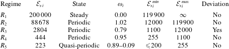
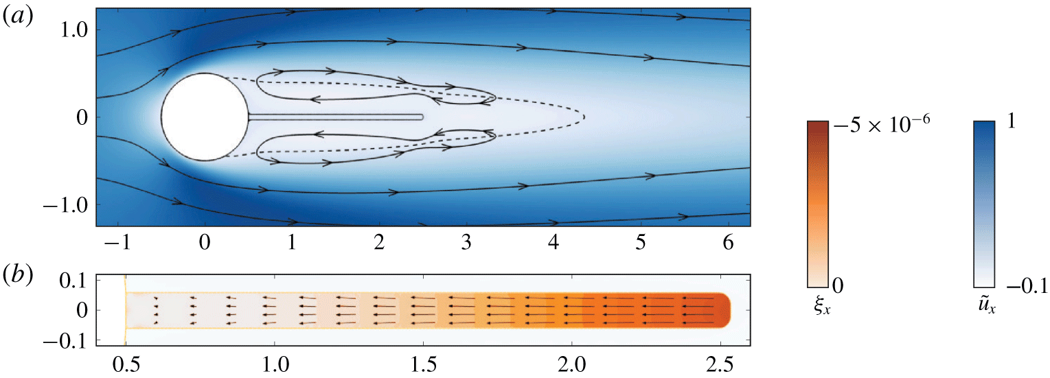
Figure 2. Regime  $R_{1}$: steady interaction of the elastic plate with the fluid flow. (a) Streamwise fluid velocity (white–blue gradient) and flow streamlines (black curves with arrows). The recirculation region is delimited by the dashed line. (b) Close-up view of the solid displacement (orange gradient), direction given by arrows.
Regime  $R_{1}$ – steady symmetric solution. A steady behaviour is observed for high values of the plate’s rigidity. A steady wake develops symmetrically around the axis $y=0$ downstream to the cylinder, while the plate is kept aligned along this symmetry axis. The steady flow obtained for ${\mathcal{E}}_{s}={{\mathcal{E}}_{s}}_{1}$ (see table 1) is shown in figure 2. The fluid flow is represented in (a), where the black solid lines indicate a few streamlines. The flow detaches from the cylinder surface and forms two symmetric recirculating regions above and below the splitter plate. Since the splitter plate surface completely lies inside the backflow region (delimited by the dashed line), the shear stress generated by the fluid is directed upstream. As a consequence, the solid is slightly compressed, as shown in (b). The displacement field is oriented almost exclusively along the $x$ axis, but a slight flare in the direction of the $\pm y$ axis is observed as one moves closer to the clamped edge of the plate, due to the positive Poisson effect ( $\unicode[STIX]{x1D708}_{s}=0.35$). The amplitude of the compression is rather small: for the case considered, the tip end streamwise displacement is only $-5\times 10^{-6}$.
Regime  $R_{2}$ – symmetric and periodic oscillation. When decreasing the rigidity below the critical value ${\mathcal{E}}_{s}=119\,900$, unsteady oscillations appear. A typical solution is reported in figure 3 for a stiffness parameter ${{\mathcal{E}}_{s}}_{2}=88\,678$. The transverse tip displacement of the splitter plate as well as the total lift coefficient (exerted on the cylinder and splitter plate) are shown as a function of time at the top. For $t>175$ an oscillation develops and grows exponentially, before saturating in a periodic limit cycle for $t>300$. We observe that the plate exhibits large displacements (more than half the cylinder’s diameter at the plate’s tip). The frequency spectrum, computed for the lift signal and displayed in figure 7(a), shows a single peak at the fundamental circular frequency $\unicode[STIX]{x1D714}_{2}\simeq 1.02$.
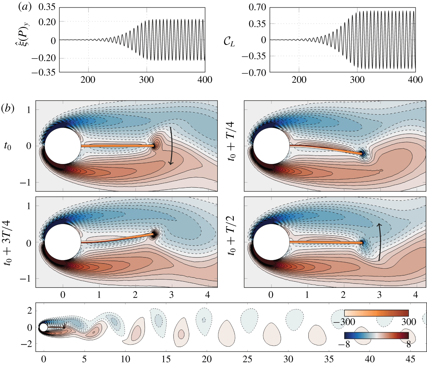
Figure 3. Regime  $R_{2}$: symmetric and periodic fluid–structure interaction obtained for ${{\mathcal{E}}_{s}}_{2}=88\,678$. (a) Temporal evolution of the transverse tip displacement $\unicode[STIX]{x1D743}(P)_{y}$ and of the lift coefficient ${\mathcal{C}}_{L}$. (b) Plot of the $z$ vorticity (blue–red colours, dashed negative contours) in the fluid and of the $yy$ stress in the solid (orange colour). Black arrows indicate the direction of the space-averaged velocity vector in the solid.
Snapshots of the fluid–structure solutions (flow vorticity and  $yy$ solid stress component) are displayed in figure 3(b). Two shear layers of opposite sign emerge from the top and bottom faces of the rigid cylinder, and vortices are shed further downstream in the wake, as seen in the overall bottom picture. The splitter plate clearly interacts with the shedding of large vortices that occur near the tip of the plate, and may act as a ‘vortex cutter’ promoting the vortex shedding. Examining more carefully the flow around the plate, secondary smaller vortices are visible around the plate’s tip during its motion, with a positive sign as the plate goes downwards (upper left picture) and a negative sign as the plate goes upwards (lower right picture). They do not have a sufficient strength to be released in the wake and stay attached, but the resulting downwash (or upwash) effect is sufficient to affect the larger, surrounding vortices.
Regime  $R_{3}$ – deviated and periodic oscillation. When rigidity is further decreased below ${\mathcal{E}}_{s}=12\,000$, a new regime appears for which the plate oscillates around a position deviated from the symmetry axis $x=0$. For the solution displayed in figure 4 ( ${{\mathcal{E}}_{s}}_{3}=2804$), the plate is deviated towards the bottom but deviated solutions towards the top may be obtained for other meshes or initial conditions. The mean deviation is clearly visible in the temporal evolutions shown in figure 4(a). The tip of the plate first deviates slowly towards the bottom between $t\simeq 100$ and $t\simeq 200$, which goes together with the appearance of negative lift, as already observed in previous numerical studies (Lacis et al. Reference Lacis, Brosse, Ingremeau, Mazzino, Lundell, Kellay and Bagheri2014; Bagheri et al. Reference Bagheri, Mazzino and Bottaro2012). For $200\leqslant t\leqslant 600$, the displacement and lift signals do not oscillate, as if the solution had reached a steady state. However, for $t>600$, unsteady oscillations appear, grow exponentially and saturate in a periodic limit cycle for $t>750$. The spectrum for the lift signal, reported in figure 7(b), shows one fundamental frequency at $\unicode[STIX]{x1D714}_{3}=0.79$ and one harmonic peak at $2\unicode[STIX]{x1D714}_{3}$. Note that a peak is obtained at $2\unicode[STIX]{x1D714}_{3}$ (and not $3\unicode[STIX]{x1D714}$ as in the previous case) because the plate ceases to oscillate about the symmetric position, so that the lift and drag coefficients have now the same periodicity. The amplitude of the vibrations is much smaller than in regime $R_{2}$. The mean deviation has thus a strong stabilizing effect on the wake oscillation. The drag (not shown) is also reduced. In figure 4(b), snapshots of vorticity in the deviated limit cycle are reported. The mean position of the plate is always maintained in the $y<0$ region (which corresponds to a negative lift), on top of which small oscillations are superimposed. Vortices are shed, but with a smaller intensity than before, and further away from the plate (the shedding region is around $x\simeq 10$, as compared to $x\simeq 5$ in the previous case). All goes as if the seemingly more streamlined overall shape prevents the release of vortices in the wake.
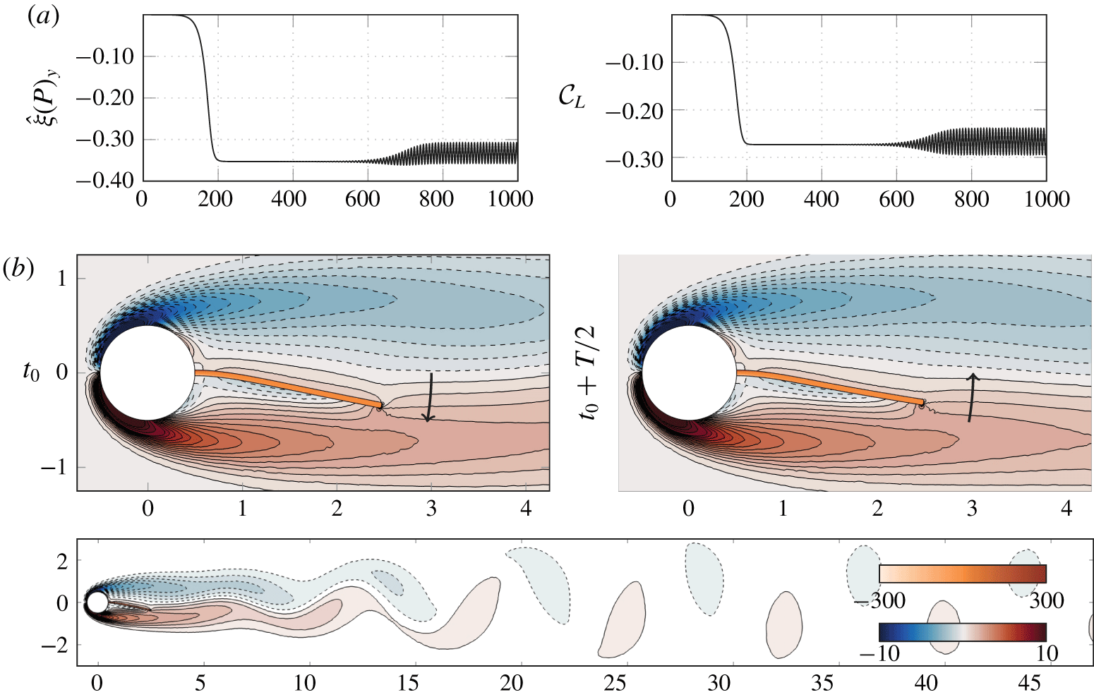
Figure 4. Regime  $R_{3}$: deviated periodic solution for ${{\mathcal{E}}_{s}}_{3}=2804$. (a) Temporal evolution of the transverse tip displacement $\unicode[STIX]{x1D743}(P)_{y}$ and of the lift coefficient ${\mathcal{C}}_{L}$. (b) Plot of the $z$ vorticity (blue–red colours, dashed negative contours) in the fluid and of the $yy$ stress in the solid (orange colour). Black arrows indicate the direction of the space-averaged velocity vector in the solid.
Regime  $R_{4}$ – back to symmetric and periodic oscillations. When further decreasing the rigidity below ${\mathcal{E}}_{s}=1100$, the mean deviation disappears. The main characteristics of this solution are reported in figure 5 obtained for ${{\mathcal{E}}_{s}}_{4}=444$. The symmetric deformation of the plate follows a different pattern than the one obtained in regime $R_{2}$. Indeed, an inflexion point appears in the centreline deformation of the plate, and the maximal transverse deviation is increased. Despite this increase of the oscillation amplitude, the lift amplitude is reduced compared to the case ${\mathcal{E}}_{s}={{\mathcal{E}}_{s}}_{2}$, probably because the kinematics of the plate decreases the strength of the vortex release. The spectrum of the lift signal is reported in figure 7(c). The largest peak of response is located at $\unicode[STIX]{x1D714}_{4}\simeq 0.95$. Because of the recovered symmetry, the harmonics are obtained at frequencies $3\unicode[STIX]{x1D714}_{4}$, $5\unicode[STIX]{x1D714}_{4}$, etc.
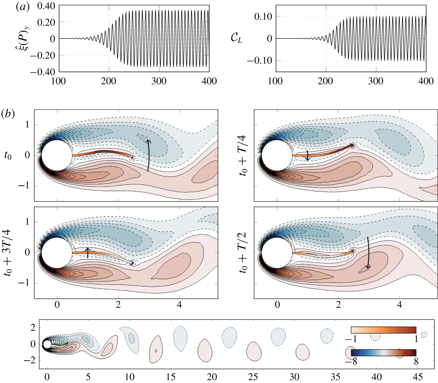
Figure 5. Regime  $R_{4}$: symmetric and periodic oscillation obtained for ${{\mathcal{E}}_{s}}_{4}=444$. (a) Temporal evolution of the transverse tip displacement $\unicode[STIX]{x1D743}(P)_{y}$ and of the lift coefficient ${\mathcal{C}}_{L}$. (b) Plot of the $z$ vorticity (blue–red colours, dashed negative contours) in the fluid and of the $yy$ stress in the solid (orange colour). Black arrows indicate the direction of the space-averaged velocity vector in the solid.
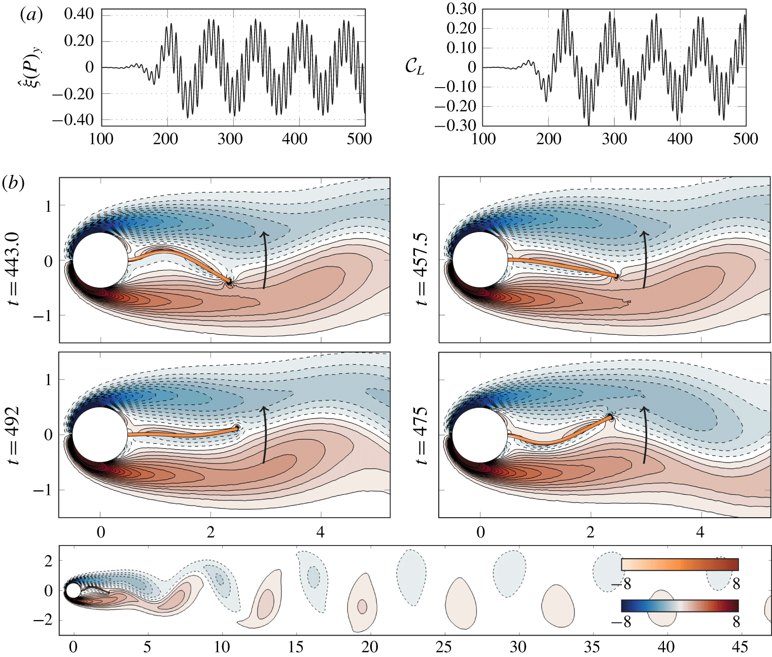
Figure 6. Regime  $R_{5}$: symmetry and quasi-periodic oscillation, obtained for ${{\mathcal{E}}_{s}}_{5}=223$. (a) Temporal evolution of the transverse tip displacement $\unicode[STIX]{x1D743}(P)_{y}$ and of the lift coefficient ${\mathcal{C}}_{L}$. (b) Plot of the $z$ vorticity (blue–red colours, dashed negative contours) in the fluid and of the $yy$ stress in the solid (orange colour). Black arrows indicate the direction of the velocity vector in the solid, averaged over the high-frequency period.
Regime  $R_{5}$ – symmetric and quasi-periodic oscillations. Finally, for the lower values of rigidity explored in the present study, another regime of unsteady symmetric solutions is observed, shown in figure 6 for ${{\mathcal{E}}_{s}}_{5}=223$. The high-frequency oscillation is now superposed to a secondary low-frequency oscillation that is clearly visible in the temporal signals as well as in the spectrum (figure 7d). The high frequency $\unicode[STIX]{x1D714}_{5}=0.89$ is close to the vortex-shedding frequency found in the previous periodic regimes, while the secondary frequency $\unicode[STIX]{x1D714}_{5}^{(2)}=0.09$ is almost ten times lower. The vibration pattern in the solid is very different from what was observed previously, its movement is now composed of a combination of bending with one and two vibration nodes.
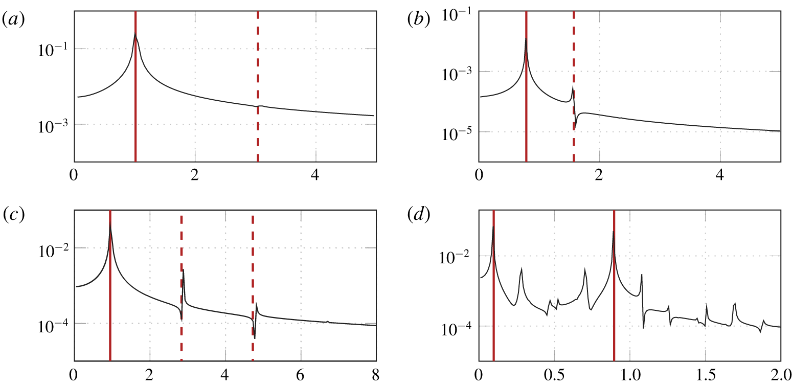
Figure 7. Frequency spectra. Plot of the fast Fourier transform spectra of the lift coefficient  ${\mathcal{C}}_{L}$ for the time-marching simulations with (a) ${{\mathcal{E}}_{s}}_{2}=88\,678$, (b) ${{\mathcal{E}}_{s}}_{3}=2804$, (c) ${{\mathcal{E}}_{s}}_{4}=444$ and (d) ${{\mathcal{E}}_{s}}_{5}=223$. Fundamental frequencies are marked with the solid vertical line, noticeable harmonics with the dashed lines.
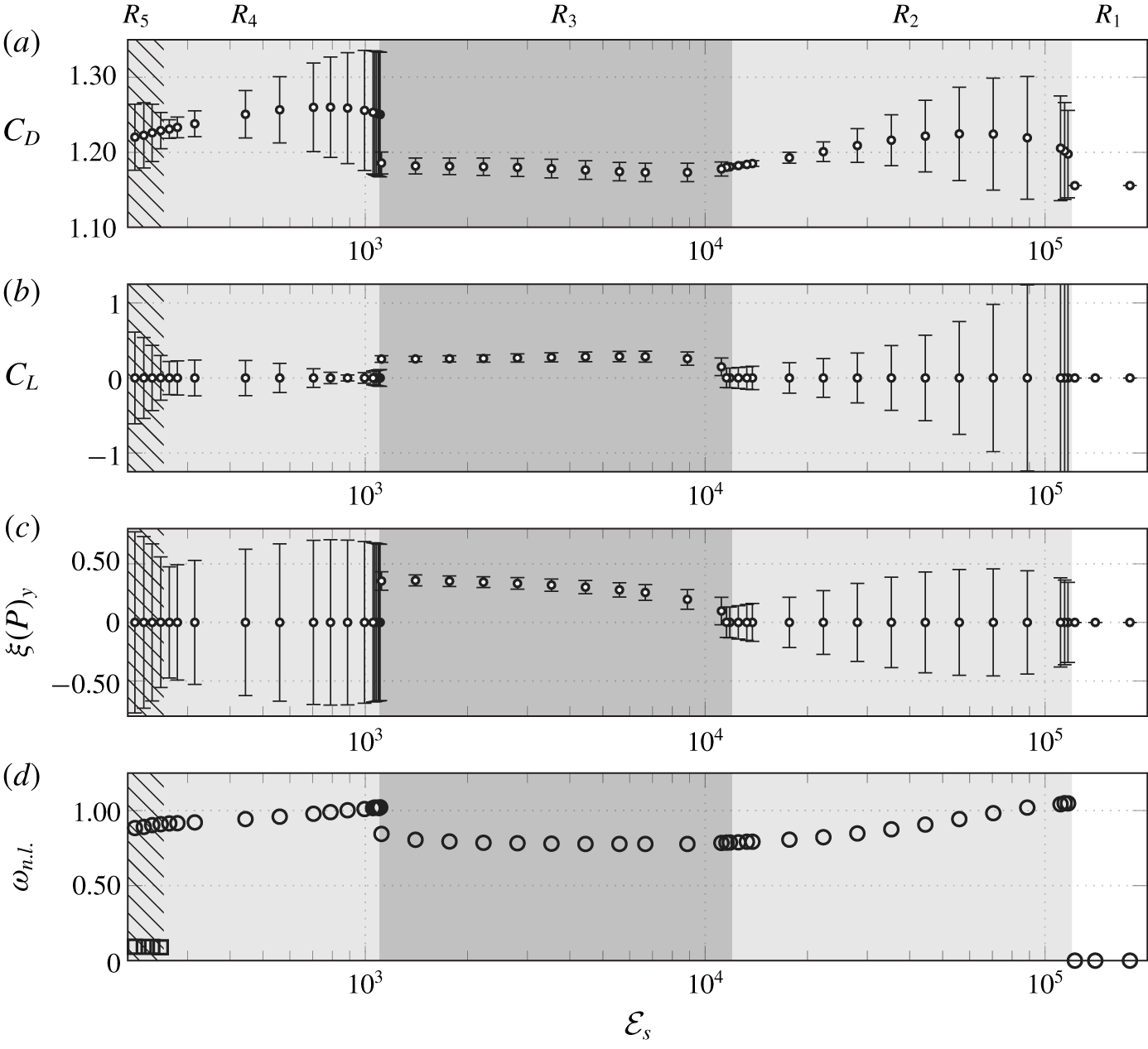
Figure 8. Characteristics of the five regimes of nonlinear interaction. For different values of  ${\mathcal{E}}_{s}$, plot of the (a) drag and (b) lift coefficients, and the (c) plate transverse tip displacement, in the limit-cycle regime. The mean value, indicated by a circle (○) symbol, is computed as $1/2\,(\max +\min )$, while the amplitude $(\max -\min )$ is indicated by the error bar and centred about the mean. The fundamental high and low frequencies (if any) are reported in (d) with ○ and ▫ symbols, respectively. Regions $R_{2}$ and $R_{4}$ are highlighted with a grey colour, while region $R_{3}$ coming with deviated mean oscillations is emphasized by a darker grey colour. Region $R_{5}$ with quasi-periodic oscillations is hatched with oblique lines.
A general overview of the five regimes is shown in figure 8, that displays in (a) the total drag coefficient, (b) the total lift coefficient, (c) the transverse displacement of the plate’s tip and (d) the fundamental frequencies of the periodic (and quasi-periodic) solutions as a function of the stiffness  ${\mathcal{E}}_{s}$. For large stiffness values (right end, region $R_{1}$), steady fluid–structure solutions are found: the plate slightly deforms and the flow remains steady and symmetric. Decreasing the rigidity below ${\mathcal{E}}_{s}=119\,900$ results in oscillating states (region $R_{2}$) with a zero-mean $y$-displacement. In this region, very large-amplitude lift fluctuations are observed, while the mean drag is increased compared to the stationary case. Note that the same behaviour was observed for the simpler case of spring-mounted cylinders where, when decreasing the stiffness (i.e. increasing the reduced velocity), one suddenly passes from a steady regime with zero lift to an unsteady regime where lift and vibration amplitudes are the highest (Zhang et al. Reference Zhang, Li, Ye and Jiang2015; Navrose & Mittal Reference Navrose and Mittal2016). Decreasing further the rigidity below ${\mathcal{E}}_{s}=12\,000$ results in oscillating states with a deviated mean transverse displacement (region $R_{3}$). This region comes with much smaller oscillation amplitudes. This region suddenly ceases to exist from ${\mathcal{E}}_{s}=1100$. A symmetric oscillating state is recovered in this region $R_{4}$, but with other flapping features than previously. Very high vibration amplitudes are reached (greater than the diameter of the cylinder), but the lift fluctuation amplitudes are smaller than in the first unsteady symmetric region. Finally, below ${\mathcal{E}}_{s}=255$, quasi-periodic limit cycles are observed (region $R_{5}$).
We have seen that several solutions can be reached by simply varying the rigidity. The transient behaviours observed suggest that the limit cycles result from the saturation of linear instabilities of the steady states. In the next section, we therefore conduct a linear stability analysis, so as to identify and characterize the various fluid–structure instabilities that may arise.
4 Results of stability analyses
4.1 Results of the exact fluid–structure stability analysis
We report here results of the fully coupled, linear fluid–structure stability analysis, first by describing the various unstable eigenmodes found, and then by characterizing the regimes of linear instability. These results are then compared to the previous results obtained with temporal simulations. Details about the numerical methods used to determine the steady nonlinear solutions of (2.1) and to compute the eigenvalues of (2.5) are given in appendix B.
Varying  ${\mathcal{E}}_{s}$ in the range $[2\times 10^{2},2\times 10^{5}]$ and keeping the other parameters fixed, we have obtained steady and symmetric solutions that are very similar to fluid–structure solutions obtained with time-marching simulations in regime $R_{1}$ (see figure 2). The axial compression in the plate increases almost linearly when ${\mathcal{E}}_{s}$ is decreased, over the whole range of rigidities. The maximal deviation to linearity is reached at small stiffness and does not exceed 0.5 %. The total drag coefficient is around ${\mathcal{C}}_{D}=1.155$ and varies less than 0.1 % over the whole range of rigidities.
By performing the stability analysis, we have identified four types of fluid–structure modes that may be unstable, labelled  $m_{i}$ ( $1\leqslant i\leqslant 4$) in the following, and summarized in table 2. Let us now describe these modes.
Table 2. The four unstable typical eigenmodes, labelled  $m_{i}$ ( $1\leqslant i\leqslant 4$), found with the linear stability analysis. The second column reports the value ${{\mathcal{E}}_{s}}_{i}$ for which each mode is displayed in the text and figures. The third and fourth columns report their growth rate $\unicode[STIX]{x1D706}_{i}^{r}$ and frequency $\unicode[STIX]{x1D706}_{i}^{i}$. The fifth and sixth columns give the minimal and maximal values of the Young modulus for which the given type of mode is unstable.
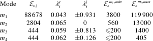
Unsteady mode  $m_{1}$. This is the first mode to get destabilized when decreasing the rigidity. The eigenvalue spectrum and the spatial structure of such mode are shown in figure 9, for the same stiffness value ${{\mathcal{E}}_{s}}_{2}=88\,678$ as that of the typical nonlinear solution in regime $R_{2}$. We observe a pair of complex-conjugate unstable modes ( $\unicode[STIX]{x1D706}^{r}>0$) in the eigenvalue spectrum, emphasized with the ○ symbol. Note that as the governing operators are real valued, the eigenvalue spectrum is necessarily symmetric with respect to the real axis (Golub & van Loan Reference Golub and van Loan2013). The real part of the corresponding eigenvector is displayed in figure 9, with contour lines representing the streamwise Eulerian velocity perturbation $\tilde{\boldsymbol{u}}^{\circ }=\boldsymbol{u}^{\circ }-\unicode[STIX]{x1D735}\boldsymbol{U}\unicode[STIX]{x1D743}_{e}^{\circ }$. Recall that this quantity represents the velocity perturbation in the perturbed domain (Fanion, Fernández & Le Tallec Reference Fanion, Fernández and Le Tallec2000; Fernández & Le Tallec Reference Fernández and Le Tallec2003) and does not depend upon the choice of the extension operator (Pfister et al. Reference Pfister, Marquet and Carini2019). This representation is actually a snapshot of the perturbation at a certain phase of the oscillation cycle. When the phase is varied, the vortex structures are advected downstream in the wake flow, while the plate’s deformation alternates up and down. This dynamical deformation is made more clear for the solid with a superposition of the plate’s position (the displacement being arbitrarily scaled) at different phases (dark lines). The perturbed position of the solid, deduced by applying the real part of the mode to its position in the steady deformed configuration, is represented by the orange line. The downwards deformation of the structure induces a positive streamwise velocity in the vicinity of the splitter plate, while the flow goes in the other direction further away in the transverse direction. The streamwise deformation of the plate is almost zero, which indicates that, at the linear level, the coupling with the solid occurs essentially through a pressure effect rather than through shear stresses. In the fluid, the characteristic features of an unstable vortex-shedding mode are found (Hill Reference Hill1992), i.e. alternate lobes of positive and negative streamwise velocity that mark the early stages of development of the unsteady Bénard–von Kármán vortex street, that was clearly visible in figure 3. The oscillation frequency of the linear mode, $\unicode[STIX]{x1D706}_{2}^{i}=0.93$, is also very close to the oscillation frequency of the nonlinear periodic solution, $\unicode[STIX]{x1D714}_{2}=1.02$. The coupled fluid–solid vibration frequency is, however, much lower than that of the lowest free solid vibration frequency of the plate $(\unicode[STIX]{x1D714}_{s,1})_{2}=4.86$ obtained by solving (2.14) at the same stiffness parameter. This indicates that strong added-mass effects are at play, that will be discussed into more detail in § 4.3.
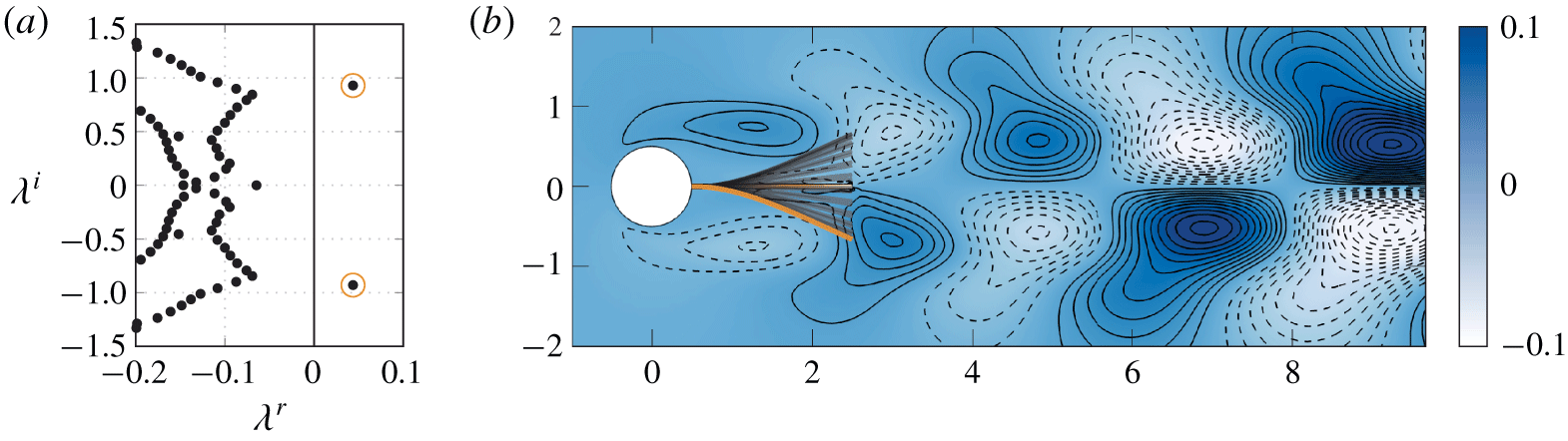
Figure 9. Unsteady mode  $m_{1}$ for ${{\mathcal{E}}_{s}}_{2}=88\,678$. (a) Eigenvalue spectrum showing one unstable pair of complex-conjugate modes ( $\unicode[STIX]{x1D706}^{r}>0$) emphasized by the ○ symbol. (b) Eulerian velocity component (blue gradient and contours, dashed negative) for the real part of the unstable eigenvector; and instantaneous positions of the elastic plate in an oscillation cycle (black), superposed on the reference configuration (orange, in background) and the deformed position according to the real part of the mode (orange, in foreground) of the plate.
Steady mode  $m_{2}$. Let us now consider a case with a stiffness ${{\mathcal{E}}_{s}}_{3}=2804$ (nonlinear regime $R_{3}$ with a mean deviation of the plate). Results are shown in figure 10. The eigenvalue spectrum exhibits one unstable eigenvalue with zero frequency ( $\unicode[STIX]{x1D706}^{i}=0$). The corresponding real mode thus grows exponentially in time without oscillating. This steady mode breaks the reflection symmetry of the symmetric steady flow around the axis $x=0$, and for that reason is called a symmetry-breaking – or divergence – instability mode. The elastic plate is deflected, here downward, but an upward deviation is obtained by reversing the arbitrary sign of this real mode. In the fluid, the spatial structure of this mode is similar to those found when investigating the dynamics of freely rising or falling bodies (see for instance Ern et al. (Reference Ern, Risso, Fabre and Magnaudet2012) for a review). Unlike unsteady modes, there is no spatial oscillation of structures in the fluid component. Large values are found in the vicinity of the elastic plate, with slowly decreasing positive (respectively negative) streamwise velocity for $y<0$ (respectively $y>0$) when progressing downstream. This is the same spatial structure as in the back to terminal velocity modes in Assemat, Fabre & Magnaudet (Reference Assemat, Fabre and Magnaudet2012) – see for instance their figure 7(a).
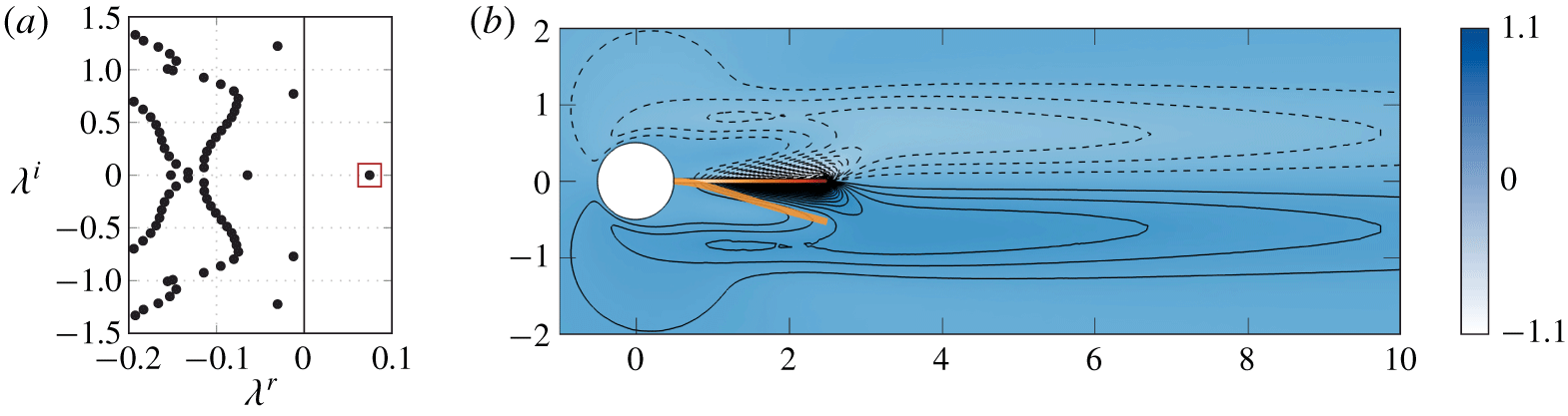
Figure 10. Steady mode  $m_{2}$ for ${\mathcal{E}}_{s}=2804$. (a) Eigenvalue spectrum showing one unstable steady mode ( $\unicode[STIX]{x1D706}^{r}>0,\unicode[STIX]{x1D706}^{i}=0$) emphasized with ▫ symbol. (b) Spatial representation of the real part of the Eulerian velocity component of the unstable mode (blue gradient and contours, dashed negative) in the steady deformed configuration, and solid deformation arbitrarily scaled (orange, thick deviated line).
Examining the velocity perturbation in figure 10, we see that it tends to decrease (respectively increase) the size of the lower (respectively upper) recirculating region in the steady symmetric solution, the signs of the steady and perturbation velocities being opposed (respectively identical). This is better visualized by plotting the superposition of the mode with the symmetric steady flow (figure 11), for two different, arbitrary values of the mode’s amplitude. The Lagrangian-based perturbation (i.e. obtained directly as eigenvector of (2.5)) is displayed here. Since it is defined in the reference configuration, we can then deform both the solid and the fluid domain according to the solid/extension perturbation field. We clearly see how the asymmetry in the mode tends to deform the recirculating region as well as to bend the splitter plate. The same type of flow and plate deformation is observed in the nonlinear regime  $R_{3}$ before the onset of oscillations.

Figure 11. Sum of the nonlinear steady solution plus the scaled – by amplitudes (a) 0.1 and (b) 0.4 – mode  $m_{2}$, for ${\mathcal{E}}_{s}=2804$. The Lagrangian-based perturbation is shown, where contours indicate negative velocity levels between 0 and $-0.15$.
High-frequency ( $m_{3}$) and low-frequency ( $m_{4}$) modes. For the lowest values of stiffness explored here, the stability analysis reveals the existence of two unstable, unsteady modes, reported in figure 12 obtained for ${{\mathcal{E}}_{s}}_{5}=223$: one oscillating at the high frequency $\unicode[STIX]{x1D706}^{i}=0.813$ (mode $m_{3}$) and one oscillating at the low frequency $\unicode[STIX]{x1D706}^{i}=0.126$ (mode $m_{4}$). For the high-frequency mode $m_{3}$, the spatial structure of the flow perturbation is typical of a vortex-shedding velocity pattern. It is very similar to that of the unsteady mode $m_{1}$ (see figure 9). However, the displacement of the elastic plate is different, as the tip of the plate is bent again in the direction of the centreline. For the low-frequency mode $m_{4}$, spatially oscillating flow perturbations are also found in the far wake (not shown here), characterized by much larger wavelengths, in agreement with the much lower oscillation frequency of this mode.
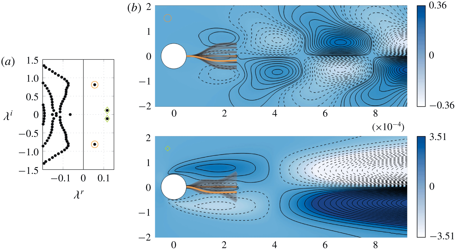
Figure 12. High-frequency and low-frequency unstable modes  $m_{3}$ and $m_{4}$ at ${\mathcal{E}}_{s}=223$. (a) Eigenvalue spectrum showing low-frequency (♢) and higher-frequency (○) unstable eigenvalues. (b) Eulerian velocity component (blue gradient and contours, dashed negative) for the real part of the unstable eigenvector; and instantaneous positions of the elastic plate in an oscillation cycle (black), superposed on the reference configuration (orange, in background) and the deformed position according to the real part of the mode (orange, in foreground) of the plate. The higher-frequency mode is at the top and the low-frequency mode at the bottom.
Effect of stiffness. The effect of a variation of the plate’s stiffness on the position of the four fluid–solid eigenmodes in the complex plane is reported in figure 13.

Figure 13. Evolution of the unstable eigenvalues in the complex plane growth rate/frequency when varying the stiffness  ${\mathcal{E}}_{s}$. Eigenvalues corresponding to (a) symmetry-breaking steady modes $m_{2}$ (▫) and low-frequency unsteady modes $m_{4}$ (♢), (b) high-frequency modes $m_{1}$ (●, orange) and (c) high-frequency modes $m_{3}$ (●, orange). The arrows indicate increasing (respectively decreasing) values of the stiffness in (a) (respectively b,c). In (b,c) the blue × symbols correspond to the modes obtained when the splitter plate is rigid, while small blue dots (●, blue) represent the evolution of the least stable hydrodynamic mode when the stiffness is decreased.
The various positions of the low-frequency  $m_{4}$ and steady $m_{2}$ eigenvalues are reported in figure 13(a), with ♢ and ▫ symbols respectively. When the stiffness is increased, the growth rate of the low-frequency modes $m_{4}$ (green circles) decreases until they become stable. Their frequency also decreases and the two complex-conjugate eigenvalues eventually collide on the zero-frequency axis $\unicode[STIX]{x1D706}^{i}=0$. Two steady eigenvalues emerge from this, one getting more and more stable, the other one being the mode $m_{2}$ that becomes unstable for ${\mathcal{E}}_{s}\geqslant 560$, before getting stable again at higher stiffness. This clearly establishes a connection between the low-frequency mode $m_{4}$ and the steady symmetry-breaking mode $m_{2}$.
The evolution of the high-frequency eigenvalues  $m_{1}$ and $m_{3}$ is depicted with ○ symbols in figures 13(b) and 13(c), respectively, now by decreasing the stiffness. In these figures, the blue crosses represent a stable branch of purely hydrodynamic modes, i.e. obtained when considering a rigid splitter plate. Among them, the least stable eigenvalue correspond to the vortex-shedding eigenmode, noted $F$. The evolution of the corresponding fluid–structure mode when decreasing the stiffness, has also been tracked and is reported with the blue circles. The modes $m_{1}$ and $m_{3}$ are both stable at high stiffness. For high values of the stiffness, their frequencies evolve according to the frequency of the structural mode that scales as ${\mathcal{E}}_{s}^{1/2}$. When the stiffness decreases so that the frequency gets closer to the frequency of the lest stable hydrodynamic mode, the two fluid–structure modes become unstable, with a frequency $\unicode[STIX]{x1D706}^{i}\sim 1.0$. Further decreasing the stiffness, the frequency of the two modes evolves towards the frequency of the hydrodynamic vortex-shedding modes. Mode $m_{1}$ is stabilized and, remarkably, it reaches the region of the spectrum in the vicinity of the (purely) hydrodynamic vortex-shedding mode. Mode $m_{3}$ remains unstable with a frequency $\unicode[STIX]{x1D706}^{i}\sim 0.8$ very close to the frequency of the (purely) hydrodynamic vortex-shedding eigenmode. To summarize, when decreasing the stiffness, the frequencies of both modes first behave as the frequency of the structural modes, until they lock to the hydrodynamic frequency. Interestingly, the mode $F$ also travels in the complex plane when the stiffness is reduced, and tends to have an increased frequency. Similar evolution of the eigenvalues has already been reported by Zhang et al. (Reference Zhang, Li, Ye and Jiang2015) and Navrose & Mittal (Reference Navrose and Mittal2016) when investigating the interaction of a spring-mounted circular cylinder with a low Reynolds number flow. We observe here the same mechanism, in the case of a more complex fluid–structure interaction – involving a flexible structure with several vibration modes.
Comparison of linear and nonlinear regimes. The growth rate and frequency of the four eigenmodes is displayed in figure 14 as a function of the stiffness. Depending on which modes are unstable, seven linear regimes of interaction are to be distinguished, referred to as  $l_{1},\ldots ,l_{7}$. The limits between these regimes are also indicated on top of the figure. Let us now compare these regions to the different nonlinear regimes observed previously. The frequency and symmetry properties of the four unstable linear modes explain some characteristics of the nonlinear regimes identified with the temporal simulations. The unsteady mode $m_{1}$ has an oscillating frequency similar to the periodic oscillations observed in regime $R_{1}$. The destabilization of the symmetry-breaking mode $m_{2}$ is coherent with time-averaged deviated solutions found in regime $R_{3}$. Finally, the coexistence of unstable low-frequency and high-frequency modes for low values of the rigidity explains the quasi-periodic solutions found in regime $R_{5}$. A comprehensive comparison is shown in figure 15, where the nonlinear regimes $R_{1},\ldots ,R_{5}$ are superimposed on the graph giving the growth rate and frequency of the linear modes. The graph at the bottom further compares the nonlinear frequencies (black circle and square symbols) and the linear frequency obtained as the imaginary part of the unstable eigenvalue (colours).
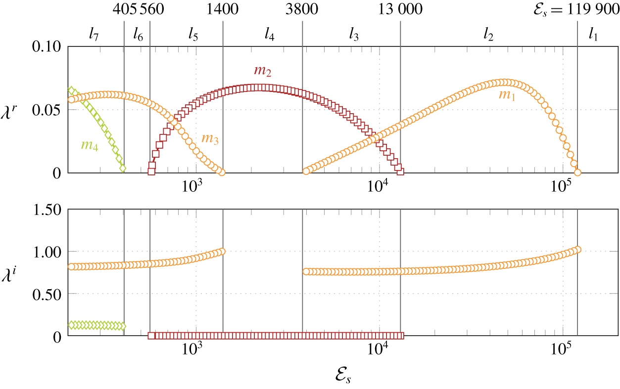
Figure 14. Eigenvalue variation with  ${\mathcal{E}}_{s}$. Evolution of the unstable eigenvalues noted $\unicode[STIX]{x1D706}=\unicode[STIX]{x1D706}^{r}+\text{i}\unicode[STIX]{x1D706}^{i}$, as a function of ${\mathcal{E}}_{s}$. Unstable, unsteady modes are depicted with orange circles (○), steady modes are depicted with red square symbols (▫) and low-frequency modes with green diamond symbols (♢). Seven regions $l_{i}$ are identified, delimited with vertical lines for which the corresponding abscissa is indicated at the top.
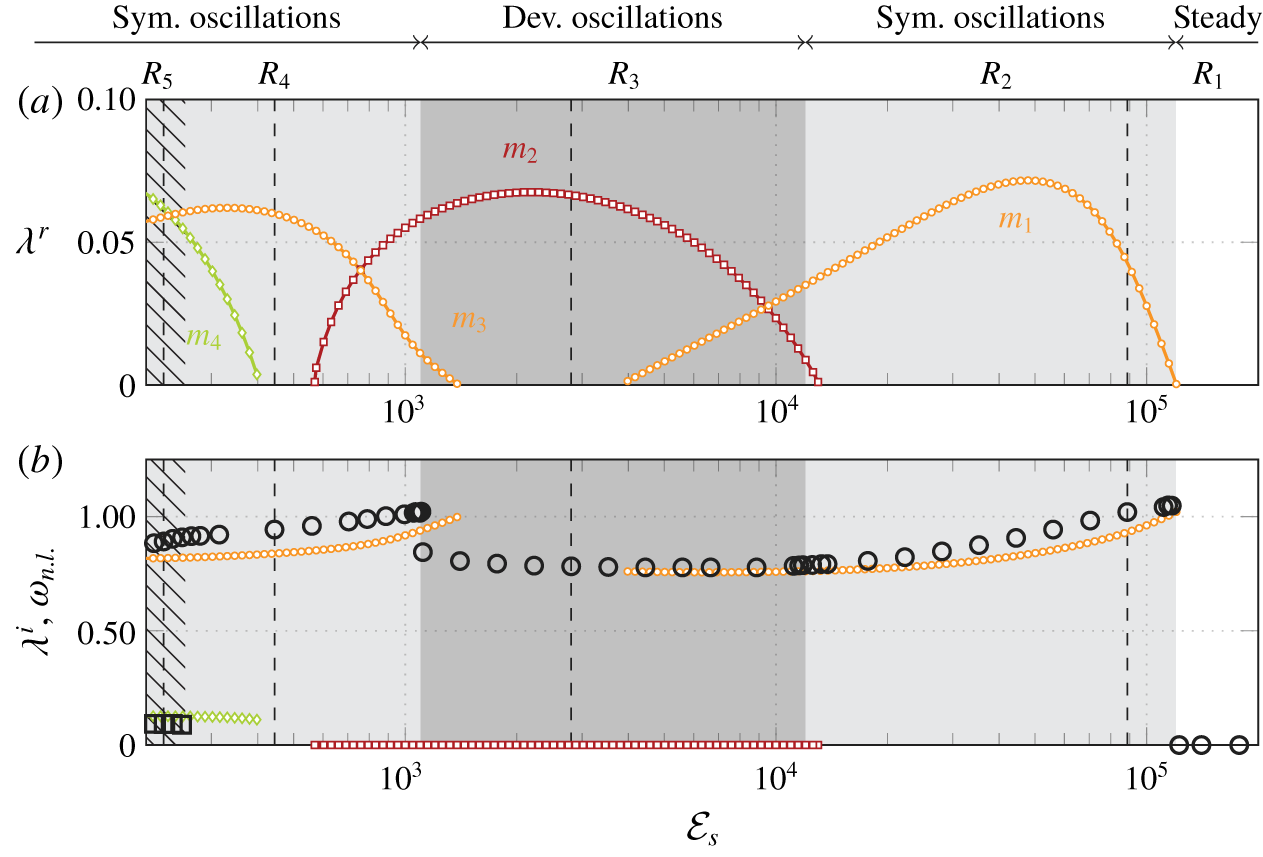
Figure 15. Comparison of linear stability results with unsteady nonlinear results. Plot of the real  $\unicode[STIX]{x1D706}^{r}$ (a) and imaginary (b) part $\unicode[STIX]{x1D706}^{i}$ for the unstable eigenvalues found by investigating the linear stability of the symmetric steady state. The values of the stiffness for the nonlinear computations are reported with a dashed line, as well as the corresponding nonlinear regimes $R_{1},\ldots ,R_{5}$. At the bottom, the largest-amplitude frequency peak $\unicode[STIX]{x1D714}_{n.l.}$ in a Fourier transform of the plate’s tip end displacement is reported with circles (○) while square symbols (▫) report (if appropriate) frequencies with a high spectrum peak that are not harmonics from the previous one.
We first examine the bifurcation between the regimes  $R_{1}$ and $R_{2}$. This threshold is perfectly captured by the stability analysis. The complex mode $m_{1}$ (○) becomes unstable at ${\mathcal{E}}_{s}=119\,900$ where a supercritical Hopf bifurcation occurs. The periodic solution observed in $R_{2}$ is the limit-cycle solution emerging from this bifurcation. Close to the threshold, the linear vibration frequency $\unicode[STIX]{x1D706}^{i}$ matches exactly the frequency of the periodic solution. A fairly good agreement between the linear and nonlinear frequencies is actually found over the whole range where the high-frequency mode $m_{1}$ is unstable: the deviation is not greater than 10 %.
We now examine the bifurcations between symmetric and non-symmetric (deviated) oscillations, that occur between regimes  $R_{2}$ and $R_{3}$ at high rigidity, and between $R_{3}$ and $R_{4}$ at lower rigidity. The steady symmetry-breaking modes $m_{3}$ (▫) are clearly related to the existence of non-symmetric oscillations in regime $R_{3}$. However, we note that the range of stiffness where this mode is unstable (encompassing linear regimes $l_{3}$, $l_{4}$ and $l_{5}$ in figure 14) does not perfectly coincide with the regime $R_{3}$. We observe three discrepancies between the linear and nonlinear results.
First, the transition between linear regimes  $l_{2}$ and $l_{3}$ where the steady mode becomes unstable occurs at ${\mathcal{E}}_{s}=13\,000$, while the bifurcation between $R_{2}$ and $R_{3}$ occurs at ${\mathcal{E}}_{s}=12\,000$. Secondly, the deviated oscillations that characterizes the regime $R_{3}$ are observed even in the linear regime $l_{4}$ where all the unsteady modes are stable and only the steady mode is unstable. This is for instance visible in the time series displayed in figure 4. A mean deviation first sets in (in agreement with the presence of a single unstable, steady mode in the eigenvalue spectrum), but then unsteady oscillations develop. This indicates the existence of secondary instabilities. Third, the stability analysis poorly predicts the bifurcation threshold ${\mathcal{E}}_{s}=1100$ between the regimes $R_{3}$ of non-symmetric oscillations and the regime $R_{4}$ of symmetric oscillations. Indeed, the steady symmetry-breaking mode is stabilized at a much lower value ${\mathcal{E}}_{s}=560$. Moreover, at the bifurcation threshold between $R_{3}$ and $R_{4}$, a sudden increase of frequency is observed in figure 15, while the linear frequency of mode $m_{3}$ decreases smoothly.
Finally, the linear analysis does not well predict the bifurcation threshold from regime  $R_{4}$ to regime $R_{5}$ where quasi-periodic oscillations appear. Indeed, the low-frequency mode gets unstable for a larger value of ${\mathcal{E}}_{s}$. Two unstable (low- and high-frequency) modes may coexist but this does not imply the onset of quasi-periodic oscillations. The latter seem to occur when the growth rate of the low-frequency mode $m_{4}$ is similar to that of the high-frequency mode $m_{3}$. However, this is only a qualitative argument. A weakly nonlinear expansion, in the spirit of Meliga, Chomaz & Sipp (Reference Meliga, Chomaz and Sipp2009) and Meliga, Gallaire & Chomaz (Reference Meliga, Gallaire and Chomaz2012), should be performed to properly determine the amplitude of each mode in the quasi-periodic solution. In particular, studying jet flows, Meliga et al. (Reference Meliga, Gallaire and Chomaz2012) performed a weakly nonlinear expansion in a case where there were two marginally stable linear modes – which was a prerequisite of their analysis – and then obtained amplitude equations describing the weakly nonlinear evolution of both modes. This kind of situation could perhaps be obtained for modes $m_{3}$ and $m_{4}$ by carefully tuning other parameters than only the stiffness. Nevertheless, as seen in the bottom figure 15, the two frequencies predicted by the linear stability analysis match well with the frequencies of the quasi-periodic solutions.
4.2 Quasi-static analysis of the steady and low-frequency modes
As observed in the previous section, there exists a connection between the steady mode  $m_{2}$ and the low-frequency mode $m_{4}$. Furthermore, both modes evolve on a time scale that is much slower than the characteristic time scale of the – stable – fluid vortex-shedding frequency (the leading eigenvalue of the fluid operator has a frequency $\unicode[STIX]{x1D714}=0.808$, see figure 13). Since these fluid–structure modes evolve on a slow time scale, the fully coupled problem (2.5) may be reduced to the quasi-static problem (2.15).
Since the plate is modelled as a purely elastic solid, the solid eigenvalue spectrum, displayed in figure 16(a), is composed of purely imaginary eigenvalues. Only the two eigenvalues of smallest frequency, labelled  $S_{1}$ and $S_{2}$, are shown in the spectrum, the corresponding modal shapes $\unicode[STIX]{x1D753}_{i}^{\circ }$ being displayed in figure 16(b). A visual comparison with the solid components of modes $m_{2}$ and $m_{4}$ (see figures 10 and 12) clearly suggest that the solid displacement can be decomposed with these two first modes as $\unicode[STIX]{x1D743}^{\circ }=\unicode[STIX]{x1D6FC}_{1}\unicode[STIX]{x1D753}_{1}^{\circ }+\unicode[STIX]{x1D6FC}_{2}\unicode[STIX]{x1D753}_{2}^{\circ }$, where the $\unicode[STIX]{x1D6FC}_{i}$ are the amplitudes of the modes. The amplitudes vector $\unicode[STIX]{x1D736}=[\unicode[STIX]{x1D6FC}_{1},\unicode[STIX]{x1D6FC}_{2}]^{\text{T}}$ is an eigenvector of the reduced eigenvalue problem (2.15), where the solid stiffness matrix $\hat{\unicode[STIX]{x1D646}}$ is diagonal with coefficients $2.659\times 10^{-4}$ and $1.034\times 10^{-2}$. The fluid added-mass, added-damping and added-rigidity matrices, are
 $$\begin{eqnarray}\hat{\unicode[STIX]{x1D648}}_{a}=\left[\begin{array}{@{}cc@{}}-73.5 & 5.22\\ -82.8 & -18.9\end{array}\right],\quad \hat{\unicode[STIX]{x1D63F}}_{a}=\left[\begin{array}{@{}cc@{}}-33.1 & -11.4\\ -25.0 & -23.3\end{array}\right],\quad \hat{\unicode[STIX]{x1D646}}_{a}=\left[\begin{array}{@{}cc@{}}3.74 & -5.02\\ 4.47 & 0.63\end{array}\right].\end{eqnarray}$$
Diagonal terms represent the added-mass, damping and stiffness effects related to individual free-vibration modes, while off-diagonal terms account for the interactions between these modes.

Figure 16. (a) Eigenvalue spectrum obtained for the solid eigenvalue problem (2.14) and (b) instantaneous displacements of the free-vibration modes  $S_{1}$ and $S_{2}$ corresponding to the two lowest frequencies displayed in (a). Results are shown for ${\mathcal{E}}_{s}=46\,800$.
A comparison of the eigenvalues obtained by solving the reduced quasi-static eigenvalue problem (2.15) and the fully coupled fluid–structure eigenvalue problem (2.1) is given in figure 17. The eigenvalues of the fully coupled problem are shown with symbols, while those of the reduced problems are displayed with the black curves.
We observe an overall good agreement between both approaches. A steady mode is found at high stiffness, that is unstable in a similar range as the steady mode  $m_{2}$. The prediction of the critical stiffness is, however, better for the upper threshold (destabilization of steady mode $m_{2}$) than for the lower thresholds (restabilization of steady modes and destabilization of low-frequency modes). This can be understood by recalling that we neglected the steady deformations of the plate ( $\boldsymbol{Q}_{s}=\boldsymbol{Q}_{e}=\mathbf{0}$) when computing the free-vibration modes used to obtain the reduced eigenvalue problem. This assumption exhibits its limits for small values of the stiffness, where the steady strains exerted by the steady flow on the plate have a non-negligible influence on the solid modes.
Secondly, when further decreasing the plate rigidity, the two steady modes merge and form a pair of complex-conjugate eigenvalues that becomes unstable, similarly to what was observed (in figure 13) for the destabilization of mode  $m_{4}$ in the fully coupled eigenvalue problem. The frequencies of these complex conjugate eigenvalues well compare to the low frequencies of modes $m_{4}$ (green symbols).
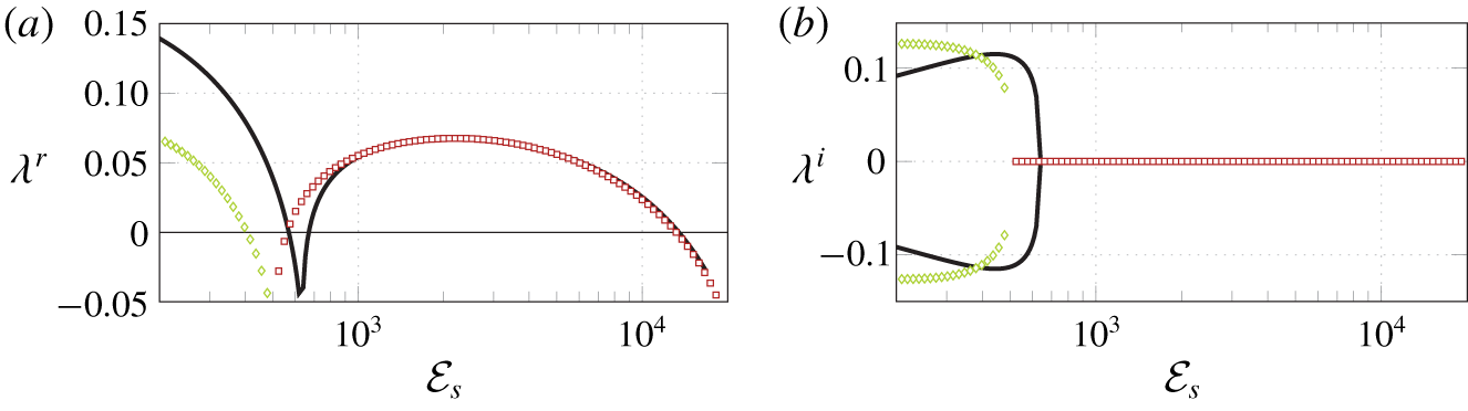
Figure 17. Comparison of the quasi-static modes found with the fully coupled analysis (symbols ▫ for the steady modes  $m_{2}$ and ♢ for the low-frequency modes $m_{4}$) and the quasi-static analysis (solid lines) with two vibration modes. (a) Growth rate and (b) frequency of the modes as a function of the Young’s modulus ${\mathcal{E}}_{s}$.
To summarize, this analysis shows that the steady instability, that appears at the high-stiffness threshold, is a divergence instability developing when the negative fluid added stiffness associated with the free-vibration mode  $S_{1}$ overcomes the restoring elastic force of the splitter plate. Thus, it is not the result of a buckling instability that would be provoked by the compression load exerted by the steady flow, since the latter has been neglected in the quasi-static analysis. The stabilization of this steady instability, followed by the onset of a low-frequency instability when decreasing the plate stiffness, results from the interaction between the free-vibration modes $S_{1}$ and $S_{2}$ through the fluid.
4.3 Quiescent-fluid analysis of the high-frequency modes
The quasi-static analysis does not allow us to capture the coupled modes  $m_{1}$ and $m_{3}$. Indeed, they correspond to oscillations of the order of the vortex-shedding frequency, as discussed previously (see figures 13 and 14). Thus, the fluid feedback now occurs on a quicker time scale so that the polynomial expansion (2.11) of the fluid resolvent is not valid anymore. It is, however, interesting to examine in that case how the fluid–structure interaction modifies the vibration dynamics, compared to that of the free-vibration case. The solid components of the coupled modes $m_{1}$ and $m_{3}$, displayed in figures 9 and 12, are close to the solid vibration modes $S_{1}$ and $S_{2}$, respectively (see figure 16 and § 4.2). Their frequencies are shown in figure 18(a) as a function of the Young’s modulus. The symbols correspond to the frequency of coupled fluid–structures modes, the grey area indicating stiffness values for which the coupled modes are unstable. The solid and dashed lines correspond to the frequency of solid vibration modes $S_{1}$ and $S_{2}$ respectively. Because the steady strains are neglected there, they evolve as ${\mathcal{E}}_{s}^{1/2}$ and thus appear as straight lines in the log–log plot. Clearly, the frequency of the coupled modes is much lower than the frequency of the solid vibration modes. For instance, for ${\mathcal{E}}_{s}=1\times 10^{4}$, the frequency of mode $m_{1}$ is twice smaller than that of the solid vibration mode $S_{1}$. In fact, the frequency of modes $m_{3}$ is closer to that of mode $S_{1}$, even if its vibration pattern is closer to that of mode $S_{2}$. Therefore, a comparison with the deformation and frequencies of the free-vibration modes is not conclusive and even misleading.
The large difference between the frequencies of the coupled and solid vibration modes can be better understood by considering the quiescent-fluid stability analysis introduced in § 2.2.2. It simply consists in solving the coupled eigenvalue problem (2.1) evaluated for a steady fluid at rest. Two stables modes of frequencies similar to modes  $m_{1}$ and $m_{3}$ have been identified and are therefore denoted $m_{1}^{0}$ and $m_{3}^{0}$. Their frequencies are reported in figure 18(b) with the solid and dashed lines. The horizontal dotted line is the vortex-shedding frequency corresponding to the purely hydrodynamic mode $\unicode[STIX]{x1D706}_{F}$.
The frequency approximation given by the quiescent-fluid modes is much better than that given by the solid vibration modes. When the coupled mode  $m_{1}$ gets unstable at high rigidity, its frequency is very well approximated by the frequency of the quiescent-fluid mode $m_{1}^{0}$. The frequency of the quiescent-fluid mode $m_{3}^{0}$ also well approximates that of the coupled mode $m_{3}$, but before the latter becomes unstable. This indicates that, before getting unstable, the frequency of the high-frequency modes $m_{1}$ and $m_{3}$ is strongly affected by the added-mass effect of the fluid. On the other hand, we also observe in figure 18(b) that, in the region of instability, the frequency of coupled modes is close to the hydrodynamic frequency (horizontal dotted line), as previously reported in figure 13(b,c). Therefore, the destabilization of the coupled modes $m_{1}$ and $m_{3}$ can be interpreted as a resonance effect between the quiescent-fluid modes and the hydrodynamics vortex-shedding mode. At the crossing between the oblique and the dotted lines, the frequency of the quiescent-fluid modes correspond to the hydrodynamic vortex-shedding frequency. The destabilization of the coupled modes clearly occurs close to these resonant frequencies. A similar scenario was reported by Zhang et al. (Reference Zhang, Li, Ye and Jiang2015) and Navrose & Mittal (Reference Navrose and Mittal2016) for the vibration of spring-mounted cylinders in low Reynolds number flows. The destabilization of a coupled mode occurred when the spring frequency (proportional to the square root of the spring stiffness) was close to the vortex-shedding frequency of the cylinder flow. The smaller the ratio between the solid and the fluid, the larger the interaction and the resonance region. The present result shows that this resonance scenario can be extended to the interaction of light elastic structures with wake flows, if the frequency of the elastic modes is corrected by the added-mass effect (quiescent-fluid modes). Finally, our result provides a new evidence that, as proposed by de Langre (Reference de Langre2006), the linear mechanism underlying the lock-in of frequencies in flow-induced vibrations/deformations can be viewed as a coupled mode flutter between hydrodynamic and structural modes.
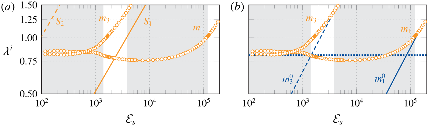
Figure 18. Modal frequencies as a function of  ${\mathcal{E}}_{s}$. (a) Frequencies of modes $m_{1}$ and $m_{3}$ (○) compared with the two first lowest free-vibration frequencies $S_{1}$ and $S_{2}$. (b) Frequencies of modes $m_{1}$ and $m_{3}$ (○) compared to frequencies of modes $m_{1}^{0}$ and $m_{3}^{0}$ obtained from the fully coupled problem with a quiescent fluid (blue oblique lines) and to the frequency of the purely hydrodynamic eigenmode (dashed horizontal line).
5 Conclusion
The dynamics of flexible splitter plates interacting with the laminar wake flow of a circular cylinder has been investigated using both nonlinear unsteady simulations and linear stability analysis. For fixed plate length  $L^{\ast }=2D^{\ast }$ and Reynolds number ${\mathcal{R}}_{e}=80$, the effect of the plate’s stiffness has been carefully examined. The nonlinear unsteady simulations are based on the arbitrary Lagrangian Eulerian formulation of the incompressible Navier–Stokes equations for modelling the flow, coupled with a Saint-Venant Kirchhoff model for the hyperelastic splitter plate. They allowed for the identification of five regimes of nonlinear interaction when decreasing the stiffness. In the first regime, the splitter plate does not oscillate and is very slightly compressed by the steady recirculating flow. In the second regime, periodic flow-induced oscillations of the splitter plate around a symmetric position are observed. In the third regime, these oscillations occur around an asymmetric position. In the fourth regime, the asymmetry has disappeared. A secondary, low frequency appears in the fifth regime, that comes with quasi-periodic oscillations.
A linear fully coupled fluid–solid stability analysis has then been considered to explain the emergence of the four regimes of self-sustained oscillations. An unstable complex eigenmode well predicts the onset and frequency of oscillations in the first regime. An unstable symmetry-breaking mode is obtained when further decreasing the stiffness, thus providing an explanation for the mechanism at the origin of the deviated oscillations. This static divergence mode becomes unstable when a negative fluid added stiffness compensates the solid restoring stiffness. Finally, the stabilization of the static mode followed by the destabilization of a low-frequency eigenmode is coherent with the existence of the quasi-periodic oscillations at low stiffness. It was observed that several features present in the linear modes are actually conserved in the nonlinear limit cycles, especially when one single mode is unstable. When two modes are unstable, other types of analyses such as weakly nonlinear expansions would be helpful in better predicting the nonlinear evolution of the perturbations. For intermediate values of the stiffness, where one of the two unstable modes is steady, it is also suggested to compute the nonlinear asymmetric steady state and to analyse its linear stability.
Finally, two simplified linear stability analyses have been derived and proposed to better characterize the destabilizing linear mechanisms at play. The quiescent-fluid analysis allows computing of the fluid added mass associated with each splitter plate’s bending mode. A resonance condition between the frequency of the (stable) vortex-shedding mode and the added-mass modes gives a good prediction of the oscillation frequency. The quasi-static linear stability analysis is appropriate to understand not only the destabilization of the symmetry-breaking mode, but also its stabilization at lower stiffness and the subsequent destabilization of the low-frequency mode.
As a perspective, we note that the present study was restricted to cases with a fixed plate length, a fixed Reynolds number and a fixed mass ratio. It would certainly be worth studying in more detail the effects of these parameters: for instance, experimental studies (conducted at higher Reynolds numbers) often considered a variation of the length of the plate rather than the stiffness. In particular, when the length of the plate is increased above a certain point, the influence of the recirculating regions decreases and the dynamics becomes mainly that of a flag. The mass ratio is also a critical parameter, that dictates the strength of dynamical couplings. Higher values of the mass ratio would certainly come with a narrower range in which vortex-induced vibration would occur, as well as the amplitude of frequency shifts compared to the free-vibration frequencies.
Acknowledgements
This project has received funding from the European Research Council (ERC) under the European Union’s Horizon 2020 research and innovation program (grant agreement no. 638307).
Declaration of interests
The authors report no conflict of interest.
Appendix A. Fluid–structure equations and operators
A.1 Nonlinear ALE fluid–solid equations
For the sake of conciseness, the governing equations (2.1) have been written in an abstract block notation, as a function of groups of variables  $\boldsymbol{q}_{s}=(\unicode[STIX]{x1D743},\boldsymbol{u}_{s})^{\text{T}}$, $\boldsymbol{q}_{e}=(\unicode[STIX]{x1D743}_{e},\unicode[STIX]{x1D740}_{e})^{\text{T}}$ and $\boldsymbol{q}_{f}=(\boldsymbol{u},p,\unicode[STIX]{x1D740})^{\text{T}}$. We provide here some details about the derivation of (2.1), and refer the reader to Pfister (Reference Pfister2019) for a comprehensive treatment. The governing nonlinear, local equations read as follows:
 $$\begin{eqnarray}\displaystyle & \displaystyle {\mathcal{M}}_{s}\frac{\unicode[STIX]{x2202}^{2}\unicode[STIX]{x1D743}}{\unicode[STIX]{x2202}t^{2}}-\unicode[STIX]{x1D735}\boldsymbol{\cdot }(\unicode[STIX]{x1D641}(\unicode[STIX]{x1D743})\unicode[STIX]{x1D64E}(\unicode[STIX]{x1D743}))=\mathbf{0}\quad \text{in}~\unicode[STIX]{x1D6FA}_{s}, & \displaystyle\end{eqnarray}$$
 $$\begin{eqnarray}\displaystyle & \displaystyle -\unicode[STIX]{x1D735}\boldsymbol{\cdot }(h_{\boldsymbol{x}}\unicode[STIX]{x1D735}\unicode[STIX]{x1D743}_{e})=\mathbf{0}\quad \text{in}~\unicode[STIX]{x1D6FA}_{e}, & \displaystyle\end{eqnarray}$$
 $$\begin{eqnarray}\displaystyle & \displaystyle \unicode[STIX]{x1D743}_{e}-\unicode[STIX]{x1D743}=\mathbf{0}\quad \text{on}~\unicode[STIX]{x1D6E4}, & \displaystyle\end{eqnarray}$$
 $$\begin{eqnarray}\displaystyle & \displaystyle J(\unicode[STIX]{x1D743}_{e})\frac{\unicode[STIX]{x2202}\boldsymbol{u}}{\unicode[STIX]{x2202}t}+(\unicode[STIX]{x1D735}\boldsymbol{u}\unicode[STIX]{x1D731}(\unicode[STIX]{x1D743}_{e}))\left(\boldsymbol{u}-\frac{\unicode[STIX]{x2202}\unicode[STIX]{x1D743}_{e}}{\unicode[STIX]{x2202}t}\right)-\unicode[STIX]{x1D735}\boldsymbol{\cdot }\unicode[STIX]{x1D72E}(\boldsymbol{u},p,\unicode[STIX]{x1D743}_{e})=\mathbf{0}\quad \text{in}~\unicode[STIX]{x1D6FA}_{f}, & \displaystyle\end{eqnarray}$$
 $$\begin{eqnarray}\displaystyle & \displaystyle -\unicode[STIX]{x1D735}\boldsymbol{\cdot }(\unicode[STIX]{x1D731}(\unicode[STIX]{x1D743}_{e})\boldsymbol{u})=0\quad \text{in}~\unicode[STIX]{x1D6FA}_{f}, & \displaystyle\end{eqnarray}$$
 $$\begin{eqnarray}\displaystyle & \displaystyle \boldsymbol{u}-\boldsymbol{u}_{s}=\mathbf{0}\quad \text{on}~\unicode[STIX]{x1D6E4}, & \displaystyle\end{eqnarray}$$
 $$\begin{eqnarray}\displaystyle & \displaystyle \unicode[STIX]{x1D72E}(\boldsymbol{u},p,\unicode[STIX]{x1D743}_{e})\boldsymbol{n}=\unicode[STIX]{x1D641}(\unicode[STIX]{x1D743})\unicode[STIX]{x1D64E}(\unicode[STIX]{x1D743})\boldsymbol{n}\quad \text{on}~\unicode[STIX]{x1D6E4}. & \displaystyle\end{eqnarray}$$
Equation (A 1) is the solid elasticity equation. Equations (A 2) and (A 3) define the extension problem. Equations (A 4) and (A 5) are the Navier–Stokes equations, rewritten in the reference domain. Finally, equations (A 6) and (A 7) express the interface velocity and stress continuity.
A.1.1 Solid sub-problem
A Saint-Venant Kirchhoff solid is considered in (A 1). The second Piola–Kirchhoff stress tensor  $\unicode[STIX]{x1D64E}$ then depends on the Green–Lagrange strain tensor $\unicode[STIX]{x1D640}$ as
 $$\begin{eqnarray}\unicode[STIX]{x1D64E}(\unicode[STIX]{x1D743})=\frac{{\mathcal{E}}_{s}}{1+\unicode[STIX]{x1D708}_{s}}\left\{\frac{\unicode[STIX]{x1D708}_{s}}{1-2\unicode[STIX]{x1D708}_{s}}\operatorname{tr}(\unicode[STIX]{x1D640}(\unicode[STIX]{x1D743}))\unicode[STIX]{x1D644}+\unicode[STIX]{x1D640}(\unicode[STIX]{x1D743})\right\},\end{eqnarray}$$
 where  $\unicode[STIX]{x1D640}=\frac{1}{2}(\unicode[STIX]{x1D641}(\unicode[STIX]{x1D743})^{\text{T}}\unicode[STIX]{x1D641}(\unicode[STIX]{x1D743})-\unicode[STIX]{x1D644})$ and $\unicode[STIX]{x1D641}(\unicode[STIX]{x1D743})=\unicode[STIX]{x1D644}+\unicode[STIX]{x1D735}\unicode[STIX]{x1D743}$ is the deformation gradient, and $\operatorname{tr}(\unicode[STIX]{x1D640})=E_{ii}$ is the trace of $\unicode[STIX]{x1D640}$. Multiplication of (A 1) by a test function and integrating by parts over $\unicode[STIX]{x1D6FA}_{s}$ then gives the variational formulation of the solid problem, that may be written as
 $$\begin{eqnarray}{\mathcal{M}}_{s}\unicode[STIX]{x1D648}_{\unicode[STIX]{x1D668}}\frac{\unicode[STIX]{x2202}^{2}\unicode[STIX]{x1D743}}{\unicode[STIX]{x2202}t^{2}}=-{\mathcal{E}}_{s}\unicode[STIX]{x1D646}_{\unicode[STIX]{x1D668}}(\unicode[STIX]{x1D743})+{\unicode[STIX]{x1D644}_{\unicode[STIX]{x1D65B}\unicode[STIX]{x1D743}}}^{\text{T}}\boldsymbol{q}_{f}.\end{eqnarray}$$
 This equation is coupled with the fluid group of variables  $\boldsymbol{q}_{f}=(\boldsymbol{u},p,\unicode[STIX]{x1D740})^{\text{T}}$ through the operator ${\unicode[STIX]{x1D644}_{\unicode[STIX]{x1D65B}\unicode[STIX]{x1D743}}}^{\text{T}}=(\unicode[STIX]{x1D7EC}\,\unicode[STIX]{x1D7EC}\,{\unicode[STIX]{x1D644}_{\unicode[STIX]{x1D668}}}^{\text{T}})$, because the fluid applies a load on the solid boundary $\unicode[STIX]{x1D6E4}$. Formally, from the stress continuity condition (A 7), the interface solid stress $\unicode[STIX]{x1D641}(\unicode[STIX]{x1D743})\unicode[STIX]{x1D64E}(\unicode[STIX]{x1D743})\boldsymbol{n}$ resulting from the integration by parts of (A 1) is identified with the interface fluid stress $\unicode[STIX]{x1D740}=\unicode[STIX]{x1D72E}(\boldsymbol{u},p,\unicode[STIX]{x1D743}_{e})\boldsymbol{n}$, the normal $\boldsymbol{n}$ being taken as pointing outside the solid domain. The operators involved read as follows:
 $$\begin{eqnarray}\displaystyle & \displaystyle \langle \unicode[STIX]{x1D74D}_{s}^{\boldsymbol{u}},\unicode[STIX]{x1D648}_{\unicode[STIX]{x1D668}}\unicode[STIX]{x1D743}\rangle =\int _{\unicode[STIX]{x1D6FA}_{s}}\unicode[STIX]{x1D743}\boldsymbol{\cdot }\unicode[STIX]{x1D74D}_{s}^{\boldsymbol{u}}\,\text{d}\unicode[STIX]{x1D6FA}, & \displaystyle \nonumber\\ \displaystyle & \displaystyle \langle \unicode[STIX]{x1D74D}_{s}^{\boldsymbol{u}},\unicode[STIX]{x1D646}_{\unicode[STIX]{x1D668}}(\unicode[STIX]{x1D743})\rangle =\frac{1}{1+\unicode[STIX]{x1D708}_{s}}\int _{\unicode[STIX]{x1D6FA}_{s}}\unicode[STIX]{x1D641}(\unicode[STIX]{x1D743})\left\{\frac{\unicode[STIX]{x1D708}_{s}}{1-2\unicode[STIX]{x1D708}_{s}}\operatorname{tr}(\unicode[STIX]{x1D640}(\unicode[STIX]{x1D743}))\unicode[STIX]{x1D644}+\unicode[STIX]{x1D640}(\unicode[STIX]{x1D743})\right\}\boldsymbol{ : }\unicode[STIX]{x1D735}\unicode[STIX]{x1D74D}_{s}^{\boldsymbol{u}}\,\text{d}\unicode[STIX]{x1D6FA}, & \displaystyle \nonumber\\ \displaystyle & \displaystyle \langle \unicode[STIX]{x1D74D}^{\unicode[STIX]{x1D740}},\unicode[STIX]{x1D644}_{\unicode[STIX]{x1D668}}\unicode[STIX]{x1D743}\rangle =\int _{\unicode[STIX]{x1D6E4}}\unicode[STIX]{x1D74D}^{\unicode[STIX]{x1D740}}\boldsymbol{\cdot }\unicode[STIX]{x1D743}\,\text{d}\unicode[STIX]{x1D6E4}. & \displaystyle \nonumber\end{eqnarray}$$
 For convenience, a solid problem first order in time is preferred. Introducing the solid velocity  $\boldsymbol{u}_{s}=\unicode[STIX]{x2202}\unicode[STIX]{x1D743}/\unicode[STIX]{x2202}t$ and noting $\boldsymbol{q}_{s}=(\unicode[STIX]{x1D743},\boldsymbol{u}_{s})$, equation (A 9) is easily rewritten as $\unicode[STIX]{x1D63D}_{\boldsymbol{s}}\unicode[STIX]{x2202}_{t}\boldsymbol{q}_{s}=\unicode[STIX]{x1D63C}_{\unicode[STIX]{x1D668}}(\boldsymbol{q}_{s})+{\unicode[STIX]{x1D644}_{\unicode[STIX]{x1D65B}\unicode[STIX]{x1D668}}}^{\text{T}}\boldsymbol{q}_{f}$ – first line of (2.1) – where
 $$\begin{eqnarray}\unicode[STIX]{x1D63D}_{\boldsymbol{s}}=\left(\begin{array}{@{}cc@{}}\unicode[STIX]{x1D648}_{\unicode[STIX]{x1D668}} & \unicode[STIX]{x1D7EC}\\ \unicode[STIX]{x1D7EC} & {\mathcal{M}}_{s}\unicode[STIX]{x1D648}_{\unicode[STIX]{x1D668}}\end{array}\right),\quad \unicode[STIX]{x1D63C}_{\unicode[STIX]{x1D668}}(\boldsymbol{q}_{s})=\left(\begin{array}{@{}c@{}}\unicode[STIX]{x1D648}_{\unicode[STIX]{x1D668}}\boldsymbol{u}_{s}\\ -{\mathcal{E}}_{s}\unicode[STIX]{x1D646}_{\unicode[STIX]{x1D668}}(\unicode[STIX]{x1D743})\end{array}\right),\quad \unicode[STIX]{x1D644}_{\unicode[STIX]{x1D65B}\unicode[STIX]{x1D668}}=\left(\begin{array}{@{}cc@{}}\unicode[STIX]{x1D7EC} & \unicode[STIX]{x1D644}_{\unicode[STIX]{x1D65B}\unicode[STIX]{x1D743}}\end{array}\right).\end{eqnarray}$$
A.1.2 Extension sub-problem
In the same way, integration by parts of (A 2) with  $\unicode[STIX]{x1D743}_{e}(\boldsymbol{x},t)=\mathbf{0}$ on $\unicode[STIX]{x2202}\unicode[STIX]{x1D6FA}_{e}\setminus \unicode[STIX]{x1D6E4}$ results in a volume stiffness term and an interface term $\unicode[STIX]{x1D740}_{e}=h_{\boldsymbol{x}}\unicode[STIX]{x1D735}\unicode[STIX]{x1D743}_{e}\boldsymbol{n}$ defined on $\unicode[STIX]{x1D6E4}$ only, that is used as a Lagrange multiplier to enforce the displacement continuity condition (A 3). The extension sub-problem reads $\unicode[STIX]{x1D63C}_{\unicode[STIX]{x1D65A}}\,\boldsymbol{q}_{e}=\unicode[STIX]{x1D644}_{\unicode[STIX]{x1D65A}\unicode[STIX]{x1D668}}\,\boldsymbol{q}_{s}$ – second line of (2.1) – with
 $$\begin{eqnarray}\unicode[STIX]{x1D63C}_{\unicode[STIX]{x1D65A}}=\left(\begin{array}{@{}cc@{}}\unicode[STIX]{x1D642} & {\unicode[STIX]{x1D644}_{\unicode[STIX]{x1D65A}}}^{\text{T}}\\ \unicode[STIX]{x1D644}_{\unicode[STIX]{x1D65A}} & \unicode[STIX]{x1D7EC}\end{array}\right),\quad \unicode[STIX]{x1D644}_{\unicode[STIX]{x1D65A}\unicode[STIX]{x1D668}}=\left(\begin{array}{@{}cc@{}}\unicode[STIX]{x1D644}_{\unicode[STIX]{x1D65A}\unicode[STIX]{x1D743}} & \unicode[STIX]{x1D7EC}\end{array}\right),\quad \unicode[STIX]{x1D644}_{\unicode[STIX]{x1D65A}\unicode[STIX]{x1D743}}=\left(\begin{array}{@{}c@{}}\unicode[STIX]{x1D7EC}\\ \unicode[STIX]{x1D644}_{\unicode[STIX]{x1D668}}\end{array}\right),\end{eqnarray}$$
where the operators involved are defined as follows,
 $$\begin{eqnarray}\langle \unicode[STIX]{x1D74D}_{e}^{\boldsymbol{u}},\unicode[STIX]{x1D642}\unicode[STIX]{x1D743}_{e}\rangle =\int _{\unicode[STIX]{x1D6FA}_{f}}h_{\boldsymbol{x}}\unicode[STIX]{x1D735}\unicode[STIX]{x1D743}_{e}\boldsymbol{ : }\unicode[STIX]{x1D735}\unicode[STIX]{x1D74D}_{e}^{\boldsymbol{u}}\text{d}\unicode[STIX]{x1D6FA}\quad \text{and}\quad \langle \unicode[STIX]{x1D74D}_{e}^{\unicode[STIX]{x1D740}},\unicode[STIX]{x1D644}_{\unicode[STIX]{x1D65A}}\unicode[STIX]{x1D743}_{e}\rangle =\int _{\unicode[STIX]{x1D6E4}}\unicode[STIX]{x1D743}_{e}\boldsymbol{\cdot }\unicode[STIX]{x1D74D}_{e}^{\unicode[STIX]{x1D740}}\,\text{d}\unicode[STIX]{x1D6E4}.\end{eqnarray}$$
 Note that the choice of the extension equation (A 2) is arbitrary. We have chosen here a weighted Laplace equation (Stein, Tezduyar & Benney Reference Stein, Tezduyar and Benney2003) with  $h_{\boldsymbol{x}}$ a pseudo-stiffness field, defined as the squared inverse of the local mesh size. This enables us to propagate smoothly the interface deformation field onto the whole domain. The equation is defined in an extension domain $\unicode[STIX]{x1D6FA}_{e}$ enclosed into (but not necessarily equivalent with) the fluid domain $\unicode[STIX]{x1D6FA}_{f}$.
A.1.3 Fluid sub-problem
Equations (A 4) and (A 5) are the non-conservative ALE formulation of the Navier–Stokes equations (Le Tallec & Mouro Reference Le Tallec and Mouro2001) that govern the velocity  $\boldsymbol{u}(\boldsymbol{x},t)$ and pressure $p(\boldsymbol{x},t)$ fields defined in the reference domain $\unicode[STIX]{x1D6FA}_{f}$. The transformation to the reference domain introduces new geometric operators: the deformation operator $\unicode[STIX]{x1D731}(\unicode[STIX]{x1D743}_{e})=J(\unicode[STIX]{x1D743}_{e})\unicode[STIX]{x1D641}(\unicode[STIX]{x1D743}_{e})^{-1}$ and the Jacobian of the deformation gradient $J(\unicode[STIX]{x1D743}_{e})=\det (\unicode[STIX]{x1D641}(\unicode[STIX]{x1D743}_{e}))$, with $\unicode[STIX]{x1D641}(\unicode[STIX]{x1D743}_{e})=\unicode[STIX]{x1D644}+\unicode[STIX]{x1D735}\unicode[STIX]{x1D743}_{e}$. In the momentum equation (A 4), the convective velocity is corrected by $\unicode[STIX]{x2202}_{t}\unicode[STIX]{x1D743}_{e}$ the extension domain velocity. The fluid stress tensor reads $\unicode[STIX]{x1D72E}(\boldsymbol{u},p,\unicode[STIX]{x1D743}_{e})=\unicode[STIX]{x1D748}(\boldsymbol{u},p,\unicode[STIX]{x1D743}_{e})\unicode[STIX]{x1D731}(\unicode[STIX]{x1D743}_{e})^{\text{T}}$, where $\unicode[STIX]{x1D748}(\boldsymbol{u},p,\unicode[STIX]{x1D743}_{e})=-p\unicode[STIX]{x1D644}+2/{\mathcal{R}}_{e}\unicode[STIX]{x1D63F}(\boldsymbol{u},\unicode[STIX]{x1D743}_{e})$, and $\unicode[STIX]{x1D63F}$ is the viscous dissipation tensor,
 $$\begin{eqnarray}\displaystyle \unicode[STIX]{x1D63F}(\boldsymbol{u},\unicode[STIX]{x1D743}_{e})=\frac{1}{2}\frac{1}{J(\unicode[STIX]{x1D743}_{e})}((\unicode[STIX]{x1D735}\boldsymbol{u})\unicode[STIX]{x1D731}(\unicode[STIX]{x1D743}_{e})+\unicode[STIX]{x1D731}(\unicode[STIX]{x1D743}_{e})^{\text{T}}(\unicode[STIX]{x1D735}\boldsymbol{u})^{\text{T}}). & & \displaystyle\end{eqnarray}$$
As previously, the variational formulation of these equations is written, combined with (A 6), in the form of
 $$\begin{eqnarray}-\unicode[STIX]{x1D63D}_{\unicode[STIX]{x1D65B}\unicode[STIX]{x1D65A}}(\boldsymbol{q}_{f},\boldsymbol{q}_{e})\frac{\unicode[STIX]{x2202}\boldsymbol{q}_{e}}{\unicode[STIX]{x2202}t}+\unicode[STIX]{x1D63D}_{\unicode[STIX]{x1D65B}}(\boldsymbol{q}_{e})\frac{\unicode[STIX]{x2202}\boldsymbol{q}_{f}}{\unicode[STIX]{x2202}t}=\unicode[STIX]{x1D63C}_{\unicode[STIX]{x1D65B}}(\boldsymbol{q}_{f},\boldsymbol{q}_{e})+\unicode[STIX]{x1D644}_{\unicode[STIX]{x1D65B}\unicode[STIX]{x1D668}}\boldsymbol{q}_{s},\end{eqnarray}$$
 which is the last line of the fully coupled problem (2.1). In the above equation,  $\unicode[STIX]{x1D63D}_{\unicode[STIX]{x1D65B}}$ and $\unicode[STIX]{x1D63C}_{\unicode[STIX]{x1D65B}}$ are the Navier–Stokes operators in the reference configuration, while $\unicode[STIX]{x1D63D}_{\unicode[STIX]{x1D65B}\unicode[STIX]{x1D65A}}$ is related to the modified domain convection velocity. More precisely,
 $$\begin{eqnarray}\displaystyle \unicode[STIX]{x1D63D}_{\unicode[STIX]{x1D65B}}(\boldsymbol{q}_{f})=\left(\begin{array}{@{}ccc@{}}\unicode[STIX]{x1D648}_{\unicode[STIX]{x1D65B}}(\unicode[STIX]{x1D743}_{e}) & \unicode[STIX]{x1D7EC} & \unicode[STIX]{x1D7EC}\\ \unicode[STIX]{x1D7EC} & \unicode[STIX]{x1D7EC} & \unicode[STIX]{x1D7EC}\\ \unicode[STIX]{x1D7EC} & \unicode[STIX]{x1D7EC} & \unicode[STIX]{x1D7EC}\end{array}\right),\quad \unicode[STIX]{x1D63D}_{\unicode[STIX]{x1D65B}\unicode[STIX]{x1D65A}}(\boldsymbol{q}_{f},\boldsymbol{q}_{e})=\left(\begin{array}{@{}cc@{}}\unicode[STIX]{x1D649}(\unicode[STIX]{x1D743}_{e},\boldsymbol{u}) & \unicode[STIX]{x1D7EC}\\ \unicode[STIX]{x1D7EC} & \unicode[STIX]{x1D7EC}\\ \unicode[STIX]{x1D7EC} & \unicode[STIX]{x1D7EC}\end{array}\right), & & \displaystyle \nonumber\\ \displaystyle \unicode[STIX]{x1D63C}_{\unicode[STIX]{x1D65B}}(\boldsymbol{q}_{f},\boldsymbol{q}_{e})=\left(\begin{array}{@{}c@{}}-\unicode[STIX]{x1D649}(\unicode[STIX]{x1D743}_{e},\boldsymbol{u})\boldsymbol{u}+\unicode[STIX]{x1D63D}(\unicode[STIX]{x1D743}_{e})^{\text{T}}p-{\displaystyle \frac{2}{{\mathcal{R}}_{e}}}\unicode[STIX]{x1D63F}(\unicode[STIX]{x1D743}_{e})\boldsymbol{u}-{\unicode[STIX]{x1D644}_{\unicode[STIX]{x1D65B}}}^{\text{T}}\unicode[STIX]{x1D740}\\ \unicode[STIX]{x1D63D}(\unicode[STIX]{x1D743}_{e})\boldsymbol{u}\\ -\unicode[STIX]{x1D644}_{\unicode[STIX]{x1D65B}}\boldsymbol{u}\end{array}\right), & & \displaystyle \nonumber\end{eqnarray}$$
with
 $$\begin{eqnarray}\displaystyle & \displaystyle \langle \unicode[STIX]{x1D74D}^{\boldsymbol{u}},\unicode[STIX]{x1D648}_{\unicode[STIX]{x1D65B}}(\unicode[STIX]{x1D743}_{e})\boldsymbol{u}\rangle =\int _{\unicode[STIX]{x1D6FA}_{f}}J(\unicode[STIX]{x1D743}_{e})\boldsymbol{u}\boldsymbol{\cdot }\unicode[STIX]{x1D74D}^{\boldsymbol{u}}\,\text{d}\unicode[STIX]{x1D6FA},\quad \langle \unicode[STIX]{x1D713}^{p},\unicode[STIX]{x1D63D}(\unicode[STIX]{x1D743}_{e})\boldsymbol{u}\rangle =\int _{\unicode[STIX]{x1D6FA}_{f}}\unicode[STIX]{x1D731}(\unicode[STIX]{x1D743}_{e})^{\text{T}}\boldsymbol{ : }\unicode[STIX]{x1D735}\boldsymbol{u}\unicode[STIX]{x1D713}^{p}\,\text{d}\unicode[STIX]{x1D6FA}, & \displaystyle \nonumber\\ \displaystyle & \displaystyle \langle \unicode[STIX]{x1D74D}^{\boldsymbol{u}},\unicode[STIX]{x1D649}(\unicode[STIX]{x1D743}_{e},\boldsymbol{u})\boldsymbol{w}\rangle =\int _{\unicode[STIX]{x1D6FA}_{f}}\unicode[STIX]{x1D735}\boldsymbol{u}\unicode[STIX]{x1D731}(\unicode[STIX]{x1D743}_{e})\boldsymbol{w}\boldsymbol{\cdot }\unicode[STIX]{x1D74D}^{\boldsymbol{u}}\,\text{d}\unicode[STIX]{x1D6FA},\quad \langle \unicode[STIX]{x1D74D}^{\unicode[STIX]{x1D740}},\unicode[STIX]{x1D644}_{\unicode[STIX]{x1D65B}}\boldsymbol{u}\rangle =\int _{\unicode[STIX]{x1D6E4}}\boldsymbol{u}\boldsymbol{\cdot }\unicode[STIX]{x1D74D}^{\unicode[STIX]{x1D740}}\,\text{d}\unicode[STIX]{x1D6E4}, & \displaystyle \nonumber\\ \displaystyle & \displaystyle \langle \unicode[STIX]{x1D74D}^{\boldsymbol{u}},\unicode[STIX]{x1D63F}(\unicode[STIX]{x1D743}_{e})\boldsymbol{u}\rangle =\int _{\unicode[STIX]{x1D6FA}_{f}}\unicode[STIX]{x1D63F}(\boldsymbol{u},\unicode[STIX]{x1D743}_{e})\unicode[STIX]{x1D731}(\unicode[STIX]{x1D743}_{e})^{\text{T}}\boldsymbol{ : }\unicode[STIX]{x1D735}\unicode[STIX]{x1D74D}^{\boldsymbol{u}}\,\text{d}\unicode[STIX]{x1D6FA}. & \displaystyle \nonumber\end{eqnarray}$$
A.2 Linearized ALE fluid–solid equations
The linearization of (2.1) is easily achieved once the different operators are known, since they are all defined in a fixed domain. The linearized solid stiffness operator reads
 $$\begin{eqnarray}\unicode[STIX]{x1D63C}_{\unicode[STIX]{x1D668}}^{\prime }=\left(\begin{array}{@{}cc@{}}\unicode[STIX]{x1D7EC} & \unicode[STIX]{x1D648}_{\unicode[STIX]{x1D668}}\\ -\unicode[STIX]{x1D646}^{\prime } & \unicode[STIX]{x1D7EC}\end{array}\right)\quad \text{with}~\langle \unicode[STIX]{x1D74D}_{s}^{\boldsymbol{u}},\unicode[STIX]{x1D646}^{\prime }(\unicode[STIX]{x1D729})\unicode[STIX]{x1D743}^{\prime }\rangle =\int _{\unicode[STIX]{x1D6FA}_{s}}(\unicode[STIX]{x1D735}\unicode[STIX]{x1D743}^{\prime }\unicode[STIX]{x1D64E}(\unicode[STIX]{x1D729})+\unicode[STIX]{x1D641}(\unicode[STIX]{x1D729})\unicode[STIX]{x1D64E}^{\prime }(\unicode[STIX]{x1D729};\unicode[STIX]{x1D743}^{\prime }))\boldsymbol{ : }\unicode[STIX]{x1D735}\unicode[STIX]{x1D74D}_{s}^{\boldsymbol{u}}\,\text{d}\unicode[STIX]{x1D6FA},\end{eqnarray}$$
 where  $\unicode[STIX]{x1D64E}^{\prime }$ is obtained from (A 8) by taking the directional derivative in direction $\unicode[STIX]{x1D743}^{\prime }$ about the steady-state solid displacement $\unicode[STIX]{x1D729}$. In the same way, the linearized fluid operators read
 $$\begin{eqnarray}\unicode[STIX]{x1D63C}_{\unicode[STIX]{x1D65B}}^{\prime }=\left(\begin{array}{@{}ccc@{}}\displaystyle -\unicode[STIX]{x1D649}^{\prime }(\unicode[STIX]{x1D729}_{e},\boldsymbol{U})-\frac{2}{{\mathcal{R}}_{e}}\unicode[STIX]{x1D63F}(\unicode[STIX]{x1D729}_{e}) & \unicode[STIX]{x1D63D}(\unicode[STIX]{x1D729}_{e})^{\text{T}} & -{\unicode[STIX]{x1D644}_{\unicode[STIX]{x1D65B}}}^{\text{T}}\\ \unicode[STIX]{x1D63D}(\unicode[STIX]{x1D729}_{e}) & \unicode[STIX]{x1D7EC} & \unicode[STIX]{x1D7EC}\\ -\unicode[STIX]{x1D644}_{\unicode[STIX]{x1D65B}} & \unicode[STIX]{x1D7EC} & \unicode[STIX]{x1D7EC}\end{array}\right),\quad \unicode[STIX]{x1D63C}_{\unicode[STIX]{x1D65B}\unicode[STIX]{x1D65A}}^{\prime }=\left(\begin{array}{@{}cc@{}}\unicode[STIX]{x1D63C}_{u}^{\prime }(\unicode[STIX]{x1D729}_{e},\boldsymbol{U},P) & \unicode[STIX]{x1D7EC}\\ \unicode[STIX]{x1D63C}_{p}^{\prime }(\unicode[STIX]{x1D729}_{e},\boldsymbol{U}) & \unicode[STIX]{x1D7EC}\\ \unicode[STIX]{x1D7EC} & \unicode[STIX]{x1D7EC}\end{array}\right),\end{eqnarray}$$
 where  $\unicode[STIX]{x1D729}$ is the steady extension displacement, $\boldsymbol{U}$ the steady fluid velocity and $P$ the steady pressure field. The linearized advection operator reads $\unicode[STIX]{x1D649}^{\prime }(\unicode[STIX]{x1D729}_{e},\boldsymbol{U})\boldsymbol{u}^{\prime }=\unicode[STIX]{x1D649}(\unicode[STIX]{x1D729}_{e},\boldsymbol{U})\boldsymbol{u}^{\prime }+\unicode[STIX]{x1D649}(\unicode[STIX]{x1D729}_{e},\boldsymbol{u}^{\prime })\boldsymbol{U}$, and the different shape derivative sub-operators write
 $$\begin{eqnarray}\displaystyle & \displaystyle \langle \unicode[STIX]{x1D74D}^{\boldsymbol{u}},\unicode[STIX]{x1D63C}_{u}^{\prime }(\unicode[STIX]{x1D729}_{e},\boldsymbol{U},P)\unicode[STIX]{x1D743}_{e}^{\prime }\rangle =\int _{\unicode[STIX]{x1D6FA}_{f}}P\unicode[STIX]{x1D731}^{\prime }(\unicode[STIX]{x1D729}_{e};\unicode[STIX]{x1D743}_{e}^{\prime })^{\text{T}}\boldsymbol{ : }\unicode[STIX]{x1D735}\unicode[STIX]{x1D74D}^{\boldsymbol{u}}\,\text{d}\unicode[STIX]{x1D6FA}-\int _{\unicode[STIX]{x1D6FA}_{f}}\unicode[STIX]{x1D735}\boldsymbol{U}\unicode[STIX]{x1D731}^{\prime }(\unicode[STIX]{x1D729}_{e};\unicode[STIX]{x1D743}_{e}^{\prime })\boldsymbol{U}\boldsymbol{\cdot }\unicode[STIX]{x1D74D}^{\boldsymbol{u}}\text{d}\unicode[STIX]{x1D6FA} & \displaystyle \nonumber\\ \displaystyle & \displaystyle -\frac{2}{{\mathcal{R}}_{e}}\int _{\unicode[STIX]{x1D6FA}_{f}}[\unicode[STIX]{x1D63F}^{\prime }(\boldsymbol{U},\unicode[STIX]{x1D729}_{e};\unicode[STIX]{x1D743}_{e}^{\prime })\unicode[STIX]{x1D731}(\unicode[STIX]{x1D729}_{e})^{\text{T}}+\unicode[STIX]{x1D63F}(\boldsymbol{U},\unicode[STIX]{x1D729}_{e})\unicode[STIX]{x1D731}^{\prime }(\unicode[STIX]{x1D729}_{e};\unicode[STIX]{x1D743}_{e}^{\prime })^{\text{T}}]\boldsymbol{ : }\unicode[STIX]{x1D735}\unicode[STIX]{x1D74D}^{\boldsymbol{u}}\,\text{d}\unicode[STIX]{x1D6FA}, & \displaystyle \nonumber\\ \displaystyle & \displaystyle \langle \unicode[STIX]{x1D713}^{p},\unicode[STIX]{x1D63C}_{p}^{\prime }(\unicode[STIX]{x1D729}_{e},\boldsymbol{U})\unicode[STIX]{x1D743}_{e}^{\prime }\rangle =\int _{\unicode[STIX]{x1D6FA}_{f}}\unicode[STIX]{x1D713}^{p}\unicode[STIX]{x1D731}^{\prime }(\unicode[STIX]{x1D729}_{e};\unicode[STIX]{x1D743}_{e}^{\prime })^{\text{T}}\boldsymbol{ : }\unicode[STIX]{x1D735}\boldsymbol{U}\,\text{d}\unicode[STIX]{x1D6FA}. & \displaystyle \nonumber\end{eqnarray}$$
 These expressions involve the linearized deformation operator  $\unicode[STIX]{x1D731}^{\prime }(\unicode[STIX]{x1D729}_{e};\unicode[STIX]{x1D743}_{e}^{\prime })$ and the linearized diffusion operator $\unicode[STIX]{x1D63F}^{\prime }(\boldsymbol{U},\unicode[STIX]{x1D729}_{e};\unicode[STIX]{x1D743}_{e}^{\prime })$, that are expressed as
 $$\begin{eqnarray}\displaystyle & \displaystyle \unicode[STIX]{x1D731}^{\prime }(\unicode[STIX]{x1D729}_{e};\unicode[STIX]{x1D743}_{e}^{\prime })=\frac{1}{J(\unicode[STIX]{x1D729}_{e})}[(\unicode[STIX]{x1D731}(\unicode[STIX]{x1D729}_{e})^{\text{T}}\boldsymbol{ : }\unicode[STIX]{x1D735}\unicode[STIX]{x1D743}_{e}^{\prime })\unicode[STIX]{x1D731}(\unicode[STIX]{x1D729}_{e})-\unicode[STIX]{x1D731}(\unicode[STIX]{x1D729}_{e})\unicode[STIX]{x1D735}\unicode[STIX]{x1D743}_{e}^{\prime }\unicode[STIX]{x1D731}(\unicode[STIX]{x1D729}_{e})], & \displaystyle\end{eqnarray}$$
 $$\begin{eqnarray}\displaystyle & \displaystyle \unicode[STIX]{x1D63F}^{\prime }(\boldsymbol{U},\unicode[STIX]{x1D729}_{e};\unicode[STIX]{x1D743}_{e}^{\prime })=\frac{-1/2}{J(\unicode[STIX]{x1D729}_{e})^{2}}[\unicode[STIX]{x1D735}\boldsymbol{U}\unicode[STIX]{x1D731}(\unicode[STIX]{x1D729}_{e})\unicode[STIX]{x1D735}\unicode[STIX]{x1D743}_{e}^{\prime }\unicode[STIX]{x1D731}(\unicode[STIX]{x1D729}_{e})+(\unicode[STIX]{x1D735}\boldsymbol{U}\unicode[STIX]{x1D731}(\unicode[STIX]{x1D729}_{e})\unicode[STIX]{x1D735}\unicode[STIX]{x1D743}_{e}^{\prime }\unicode[STIX]{x1D731}(\unicode[STIX]{x1D729}_{e}))^{\text{T}}].\qquad & \displaystyle\end{eqnarray}$$
 Note that somewhat more compact expressions can be obtained by expressing these operators in the domain deformed by the steady displacement fields  $\unicode[STIX]{x1D729}$ and $\unicode[STIX]{x1D729}_{e}$, see Pfister et al. (Reference Pfister, Marquet and Carini2019).
Appendix B. Numerical methods
B.1 Numerical methods for the temporal simulations
The spatial discretization of the governing equations (2.1) is obtained by a continuous Galerkin finite-element method. Quadratic ( $P_{2}$) elements are used to discretize the velocity and displacement fields while linear ( $P_{1}$) elements are used for the pressure and interface Lagrange multipliers. The corresponding finite-element bases are defined on unstructured meshes obtained after Delaunay triangulation of the computation domain, that extends between $-15\leqslant x\leqslant 50$ in the streamwise direction and $-25\leqslant y\leqslant 25$ in the cross-stream direction. The mesh used for the nonlinear computations is shown in figure 19. It is composed of 29 976 triangles (15 297 vertices) among which 1376 (respectively 1007) are located in the solid region $\unicode[STIX]{x1D6FA}_{s}$. At the conforming fluid–solid interface, the grid spacing in the $x$ and $y$ directions is set to 0.0067, while the largest spacing of 1.67 is set in the far-field region. Refinement is applied in the wake up to $x=26$ so as to capture properly the wake vortices. Note that the edges of the splitter plate are not squared but rounded, with a radius 0.02. This helps to have a smooth ALE mesh generation, but is not strictly mandatory (in particular, taking straight edges does not cause special stability or convergence problems). The extension region $\unicode[STIX]{x1D6FA}_{e}$, discretized with black triangles in figure 19, is defined as a sub-region of the fluid domain, enclosing the splitter plate, with dimensions $x\in [-1.5,7]$ and $y\in [-2,2]$. The mesh is not symmetric with respect to the $x=0$ axis. A similar, symmetrized (about the axis $y=0$) mesh is used for the stability analyses.
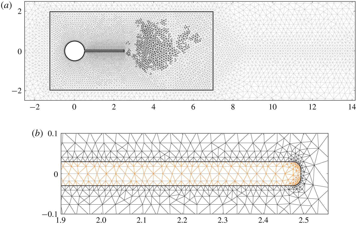
Figure 19. Plot of a typical unstructured mesh used for the spatial discretization with finite elements. (a) The discretization of the extension domain  $\unicode[STIX]{x1D6FA}_{e}$ is displayed in black while the discretization in the far-field fluid region $\unicode[STIX]{x1D6FA}_{f}$ is in light grey. Only a portion of the mesh is represented. (b) Close-up view in the vicinity of the splitter plate’s tip. The mesh in the solid region $\unicode[STIX]{x1D6FA}_{s}$ is displayed in orange.
A fully implicit temporal scheme is then used to discretize in time the fluid–structure problem (2.1). More specifically, we use the shifted Crank–Nicholson scheme proposed by Wick (Reference Wick2013b), as it offers a good compromise between low dissipation and numerical stability. At each temporal iteration, the time-discretized fully nonlinear problem derived from (2.1) is solved with a Newton method with an exact Jacobian (Wick Reference Wick2013a). The resulting sparse matrices and vectors are assembled using the software FreeFEM (Hecht Reference Hecht2012) and the resolution of the linear system at each iteration of the Newton method is performed with the distributed direct sparse solver Mumps (Amestoy et al. Reference Amestoy, Buttari, Guermouche, l’Excellent and Ucar2013). Results shown in the next paragraph have been obtained with a time step equal to  $\unicode[STIX]{x0394}t=0.01$ which was found to result in converged time series. A uniform velocity is prescribed at the inlet boundary $x=-15$, slip conditions are taken at the top and bottom far-field boundaries $y=\pm 25$ and a stress-free outflow condition is taken for the outflow at $x=50$. No-slip conditions are prescribed at the rigid boundary of the cylinder. The simulations are initialized by a uniform, zero flow. Between the non-dimensional time units $t=0$ and $t=20$ the inlet velocity is smoothly increased following the law $u_{in}(t)=0.5\,(1-\cos (\unicode[STIX]{x03C0}/20t))$, and for $t>20$ the inflow velocity is set to 1.
B.2 Numerical methods for the stability analysis
A linear stability analysis of the fluid–structure problem requires us to first determine nonlinear steady solutions of (2.1) so as to then solve the eigenvalue problem (2.5). The problems are discretized on a symmetric mesh (with respect with the axis  $y=0$). A Newton method is used to compute iteratively nonlinear steady solutions. After assembling the sparse matrices with the FreeFEM (Hecht Reference Hecht2012) software, the Mumps library (Amestoy et al. Reference Amestoy, Buttari, Guermouche, l’Excellent and Ucar2013) is used to perform the matrix inversions. When it comes to the steady flow, a uniform velocity of amplitude unity is prescribed at the inlet boundary $x=-15$, slip conditions are taken at the top and bottom far-field boundaries $y=\pm 25$ and a stress-free outflow condition is taken for the outflow at $x=50$. No-slip conditions are prescribed at the rigid boundary of the cylinder. The same boundary conditions are taken in the linearized problem, except for the inflow velocity, that is zero at the perturbation level.
The leading eigenvalue of the generalized eigenvalue problem (2.5) is then looked for with a shift-and-invert Arnoldi method using the library ARPACK (Lehoucq, Sorensen & Yang Reference Lehoucq, Sorensen and Yang1997). It requires us again to invert the Jacobian matrix in (2.6) shifted by the left-hand side matrix when computing leading eigenvalues with non-zero frequency. The solver Mumps is also used. A more detailed description of the shift-and-invert algorithm is given in Pfister et al. (Reference Pfister, Marquet and Carini2019), as well as an approach based on a block Gauss–Seidel preconditioner or modal projections, that can be used to reduce the overall memory requirements. For large-scale eigenvalue problems at moderate Reynolds numbers, the LU (lower–upper) factorization of the Jacobian fluid matrix that appears in the Gauss–Seidel loop can also be replaced by an efficient iterative solver based on the augmented Lagrangian preconditioner, as proposed by Moulin, Jolivet & Marquet (Reference Moulin, Jolivet and Marquet2019).
The nonlinear steady solver and linear eigenvalue solver used here have been validated in Pfister et al. (Reference Pfister, Marquet and Carini2019) for several fluid–structure configurations. More specifically, a configuration very similar to the present one and often used in fluid–structure interaction numerical benchmarks (Turek & Hron Reference Turek and Hron2006) has been investigated. Numerical results obtained with the stability analysis have been compared to results of nonlinear unsteady simulations, thus validating the numerical tools and the linearization approach of the fluid–structure problem. The FreeFEM scripts allowing the numerical resolutions are available on the website https://w3.onera.fr/erc-aeroflex/.


 Open access

