


1. Introduction
Vortex rings are ubiquitous across many scales, playing key roles in systems such as starting jets for propulsion (Krueger & Gharib Reference Krueger and Gharib2003), aquatic locomotion in organisms such as fish (Akanyeti et al. Reference Akanyeti, Putney, Yanagitsuru, Lauder, Stewart and Liao2017), squid (Gosline & Demont Reference Gosline and Demont1985; Anderson & DeMont Reference Anderson and DeMont2000; Bartol et al. Reference Bartol, Krueger, Stewart and Thompson2009), salps (Linden & Turner Reference Linden and Turner2004) and jellyfish (Ichikawa & Mochizuki Reference Ichikawa and Mochizuki2008; Dabiri Reference Dabiri2009; Costello et al. Reference Costello, Colin, Dabiri, Gemmell, Lucas and Sutherland2021; Gemmell et al. Reference Gemmell, Du Clos, Colin, Sutherland and Costello2021). They are also seen in respiratory flows such as coughing (Simha & Rao Reference Simha and Rao2020), and cardiac flows in the left ventricle (Pierrakos & Vlachos Reference Pierrakos and Vlachos2006). A distinguishing feature of many of these systems is that fluid is pushed out of a flexible structure which is linked to high efficiency due to the interaction of the flexible structure with the surrounding fluid (Wang et al. Reference Wang, Tang and Zhang2022). Dabiri (Reference Dabiri2009) proposed that flexible living structures, such as those found in marine animals and the heart, operate under optimal conditions of vortex formation, making them highly efficient. Therefore, understanding the dynamics and formation of isolated vortex rings generated from flexible structures could provide further insight into engineering higher efficiency systems that leverage this phenomenon.
Vortex rings are typically generated in experiments by expelling fluid through a sharp-edged nozzle or orifice into another larger body of fluid using a piston. The formation process of vortex rings from rigid nozzles has been well studied. Didden (Reference Didden1979) identified several key parameters governing vortex ring formation, including the nozzle diameter ( $D$
), the piston stroke length (
$D$
), the piston stroke length ( $L$
) and the velocity history of the piston motion
$L$
) and the velocity history of the piston motion $U_p(t)$
. For short piston stroke to diameter ratios
$U_p(t)$
. For short piston stroke to diameter ratios ${L}/{D}={U_{p}(t) t}/{D}$
, a single vortex ring forms, entraining all the expelled fluid given an impulsive piston motion. Gharib et al. (Reference Gharib, Rambod and Shariff1998) identified a limiting stroke ratio (
${L}/{D}={U_{p}(t) t}/{D}$
, a single vortex ring forms, entraining all the expelled fluid given an impulsive piston motion. Gharib et al. (Reference Gharib, Rambod and Shariff1998) identified a limiting stroke ratio ( ${L}/{D}$
) ranging from 3.6 to 4.5 below which a single vortex ring is formed, and any larger stroke ratio results in additional expelled fluid forming a trailing jet behind the vortex ring, making it a limited process. Further studies have shown that different nozzle geometries and velocity flow profiles can alter the critical
${L}/{D}$
) ranging from 3.6 to 4.5 below which a single vortex ring is formed, and any larger stroke ratio results in additional expelled fluid forming a trailing jet behind the vortex ring, making it a limited process. Further studies have shown that different nozzle geometries and velocity flow profiles can alter the critical ${L}/{D}$
value at which a vortex ring will pinch-off and no longer gain circulation (Gharib et al. Reference Gharib, Rambod and Shariff1998; Dabiri & Gharib Reference Dabiri and Gharib2005; Krieg & Mohseni Reference Krieg and Mohseni2021). Dabiri & Gharib (Reference Dabiri and Gharib2005) demonstrated that by forcing a circular nozzle exit to reduce in area as fluid was being expelled, vortex ring pinch-off could be delayed until
${L}/{D}$
value at which a vortex ring will pinch-off and no longer gain circulation (Gharib et al. Reference Gharib, Rambod and Shariff1998; Dabiri & Gharib Reference Dabiri and Gharib2005; Krieg & Mohseni Reference Krieg and Mohseni2021). Dabiri & Gharib (Reference Dabiri and Gharib2005) demonstrated that by forcing a circular nozzle exit to reduce in area as fluid was being expelled, vortex ring pinch-off could be delayed until ${L}/{D}\approx {}8$
, due to changes in the output velocity and shear layer development. Similarly, Limbourg & Nedić (Reference Limbourg and Nedić2021c
) showed that the formation process for orifice-generated vortex rings differs from those produced by a nozzle due to geometrical effects. Limbourg & Nedić (Reference Limbourg and Nedić2021a
) and Limbourg & Nedić (Reference Limbourg and Nedić2021b
) provided a correction to the traditional slug flow model to account for contraction effects at an orifice outlet, which can predict formation times that are consistent with observations for nozzle geometries. Krieg & Mohseni (Reference Krieg and Mohseni2021) found that pinch-off is determined by the characteristic velocity of the vortex ring relative to the feeding velocity of the liquid. Similar to Dabiri & Gharib (Reference Dabiri and Gharib2005), Krieg & Mohseni (Reference Krieg and Mohseni2021) showed that vortex ring pinch-off could be delayed up to a value of
${L}/{D}\approx {}8$
, due to changes in the output velocity and shear layer development. Similarly, Limbourg & Nedić (Reference Limbourg and Nedić2021c
) showed that the formation process for orifice-generated vortex rings differs from those produced by a nozzle due to geometrical effects. Limbourg & Nedić (Reference Limbourg and Nedić2021a
) and Limbourg & Nedić (Reference Limbourg and Nedić2021b
) provided a correction to the traditional slug flow model to account for contraction effects at an orifice outlet, which can predict formation times that are consistent with observations for nozzle geometries. Krieg & Mohseni (Reference Krieg and Mohseni2021) found that pinch-off is determined by the characteristic velocity of the vortex ring relative to the feeding velocity of the liquid. Similar to Dabiri & Gharib (Reference Dabiri and Gharib2005), Krieg & Mohseni (Reference Krieg and Mohseni2021) showed that vortex ring pinch-off could be delayed up to a value of $t^*\approx {}8$
for a continually accelerating feeding velocity so that the vortex ring could not outpace the feeding source. Their work provided valuable insights into predicting pinch-off timing under time varying output velocity programs.
$t^*\approx {}8$
for a continually accelerating feeding velocity so that the vortex ring could not outpace the feeding source. Their work provided valuable insights into predicting pinch-off timing under time varying output velocity programs.
Hydrodynamic impulse can be used to quantify the fluid thrust generated by a vortex ring, which is the summation of fluid impulse from the change in fluid inertia and fluid pressure (Saffman Reference Saffman1993). The total thrust supplied by a starting jet is primarily controlled by the momentum flux, and secondarily by the pressure change at the nozzle exit. The change in momentum flux is directly affected by the vortex generator as it is the integration of $\rho _{f}U_{e}^2$
, where
$\rho _{f}U_{e}^2$
, where $U_{e}$
is the fluid velocity distributed across the nozzle exit being produced by the pump or propeller and
$U_{e}$
is the fluid velocity distributed across the nozzle exit being produced by the pump or propeller and $\rho_{f}$
is the fluid density. For a rigid nozzle, this cannot be easily altered without changing the input to the system from the vortex generator. However, the pressure change,
$\rho_{f}$
is the fluid density. For a rigid nozzle, this cannot be easily altered without changing the input to the system from the vortex generator. However, the pressure change, $p - p_{\infty }$
, where
$p - p_{\infty }$
, where $p_{\infty }$
is the ambient fluid pressure, is affected by several factors including the fluid acceleration, nozzle geometry and duration of the velocity being expelled (Krueger & Gharib Reference Krueger and Gharib2003; Krieg & Mohseni Reference Krieg and Mohseni2013; Gao et al. Reference Gao, Wang, Yu and Chyu2020; Limbourg & Nedić Reference Limbourg and Nedić2021c
). These factors are all closely related to the vortex ring formation process, and help describe the increase in impulse by forming a single vortex ring. It was determined that the maximum thrust normalised by momentum flux could be achieved at
$p_{\infty }$
is the ambient fluid pressure, is affected by several factors including the fluid acceleration, nozzle geometry and duration of the velocity being expelled (Krueger & Gharib Reference Krueger and Gharib2003; Krieg & Mohseni Reference Krieg and Mohseni2013; Gao et al. Reference Gao, Wang, Yu and Chyu2020; Limbourg & Nedić Reference Limbourg and Nedić2021c
). These factors are all closely related to the vortex ring formation process, and help describe the increase in impulse by forming a single vortex ring. It was determined that the maximum thrust normalised by momentum flux could be achieved at $t^* \approx {} 4$
, for an impulsively started piston, due to the increase in pressure rise at the nozzle exit when a vortex ring pinches off (Krueger & Gharib Reference Krueger and Gharib2003). This effect has been shown to be magnified for orifice geometries due to the radial component of velocity at the edge of an orifice which is negligible in the case of a nozzle (Krieg & Mohseni Reference Krieg and Mohseni2013; Limbourg & Nedić Reference Limbourg and Nedić2021c
). Notably, thrust can also be increased with a faster fluid acceleration for the same
$t^* \approx {} 4$
, for an impulsively started piston, due to the increase in pressure rise at the nozzle exit when a vortex ring pinches off (Krueger & Gharib Reference Krueger and Gharib2003). This effect has been shown to be magnified for orifice geometries due to the radial component of velocity at the edge of an orifice which is negligible in the case of a nozzle (Krieg & Mohseni Reference Krieg and Mohseni2013; Limbourg & Nedić Reference Limbourg and Nedić2021c
). Notably, thrust can also be increased with a faster fluid acceleration for the same $t^*$
value, as would be expected based on the increased fluid momentum (Krueger & Gharib Reference Krueger and Gharib2003). Gao et al. (Reference Gao, Wang, Yu and Chyu2020) stated that the total impulse depends on the fluid deceleration as well, which can create a stopping vortex near the nozzle exit which favourably contributes to the pressure impulse. Additionally, Yin & Gad-El-Hak (Reference Yin and Gad-El-Hak2021) demonstrated that, for a pumping jet style propeller, refilling the body creates positive momentum and a stopping vortex within the body cavity.
$t^*$
value, as would be expected based on the increased fluid momentum (Krueger & Gharib Reference Krueger and Gharib2003). Gao et al. (Reference Gao, Wang, Yu and Chyu2020) stated that the total impulse depends on the fluid deceleration as well, which can create a stopping vortex near the nozzle exit which favourably contributes to the pressure impulse. Additionally, Yin & Gad-El-Hak (Reference Yin and Gad-El-Hak2021) demonstrated that, for a pumping jet style propeller, refilling the body creates positive momentum and a stopping vortex within the body cavity.
When applied to aquatic vehicles, it has been demonstrated that pulsed jet propulsion can achieve a much higher efficiency compared with steady-state jets of equivalent volume. The benefits stem from the added mass and entrainment effects from forming a series of vortex rings, which depends on formation length, fluid acceleration and Reynolds number (Siekmann Reference Siekmann1963; Krueger & Gharib Reference Krueger and Gharib2005; Dabiri Reference Dabiri2009; Moslemi & Krueger Reference Moslemi and Krueger2010, Reference Moslemi and Krueger2011; Bujard et al. Reference Bujard, Giorgio-Serchi and Weymouth2021; Baskaran & Mulleners Reference Baskaran and Mulleners2022). The increase in efficiency associated with creating sequences of vortex rings is due to a combination of increased pressure impulse per pulse as well as the interactions of each pulse with one another (Krueger & Gharib Reference Krueger and Gharib2005). However, Qin et al. (Reference Qin, Liu and Xiang2018) showed the vortex–vortex interactions of a pulsed jet could either increase circulation by as much as 10 % or reduce it by 20 % depending on the spacing of each vortex ring with one another. For instance, Xu & Dabiri (Reference Xu and Dabiri2020) showed that controlling contraction frequencies in jellyfish with micro-controllers could triple their swimming speed, while only creating a twofold increase in cost of transport, likely due to beneficial vortex interactions. In general, jet powered aquatic robotics show promise in that the impulsive motion of a starting jet can provide thrust almost instantaneously compared with several seconds for a traditional propeller to reach the desired thrust (Krieg & Mohseni Reference Krieg and Mohseni2013). This type of propulsion can enable low speed manoeuvring such as sideways translation, zero radius turns (yaw), all because there is no external fluid manipulator simply an internal jetting cavity (Krieg & Mohseni Reference Krieg and Mohseni2013). Although there are many achievements in terms of jet propelled robotics, there is limited research into the effect of utilising flexible structures to increase efficiency and maximise thrust per pulse from these types of aquatic vehicles.
Jellyfish and squid have been shown to be among the most efficient swimmers, attributed to their flexible, deformable bodies creating desirable movement kinematics (Costello et al. Reference Costello, Colin, Dabiri, Gemmell, Lucas and Sutherland2021). Jellyfish locomotion encompasses three parts: suction thrust during contraction, passive energy recapture during relaxation and a wall effect created by the interaction with counter rotating vortices left in their wake (Gemmell et al. Reference Gemmell, Du Clos, Colin, Sutherland and Costello2021). Squid exhibit similar swimming kinematics as well. Anderson et al. (2001) showed that squid utilise two distinct modes of locomotion, alternating between small bursts of fluid that create individual vortex rings, and larger jets that generate multiple vortex structures at the expense of efficiency for additional force. Xiaobo et al. (Reference Xiaobo, Wei, Qiang and Jun2021) numerically demonstrated that in the case of a soft bodied jet propulsor, with geometry similar to a squid, sucking liquid into the body has the same effect as pushing water out by increasing positive momentum within the body, which is likely related to a squid’s swimming efficiency. Numerical simulations of jellyfish revealed that synchronising contractions with the natural wave speed of the bell margin results in a maximum in thrust efficiency, related to the resonant frequency of varied stiffness bodies (Hoover et al. Reference Hoover, Xu, Gemmell, Colin, Costello, Dabiri and Miller2021).
The impact of employing flexible flaps and hinges to manipulate the flow produced by starting jets has been studied as well. Many nature-inspired researchers have shown that a specific amount of flexibility enhances thrust generation or efficiency in terms of a flapping wing or fin model (Kang et al. Reference Kang, Aono, Cesnik and Shyy2011; Marais et al. Reference Marais, Thiria, Wesfreid and Godoy-Diana2012; Dewey et al. Reference Dewey, Boschitsch, Moored, Stone and Smits2013; Park et al. Reference Park, Park, Lee, Cho and Choi2016; Medina & Kan Reference Medina and Kan2018; David et al. Reference David, Govardhan and Arakeri2019; Leroy-Calatayud et al. Reference Leroy-Calatayud, Pezzulla, Mulleners, Keiser and Reis2021; Li et al. Reference Li, Jaiman and Khoo2021). All of these studies indicate that a specific level of flexibility increases thrust production or power efficiency in flapping wing or fin models, attributed to the alignment of shed vortices and surface deformations. However, the number of studies relating flexibility to thrust generation from a starting jet is still somewhat lacking, with most findings showing that indefinitely decreasing stiffness increases thrust efficiency. Das et al. (Reference Das, Govardhan and Arakeri2018) showed that flexible flaps installed at the outlet of a rectangular channel could amplify fluid impulse by a factor of two while utilising the same energy input, due to rearrangement of vorticity of the jet. Jung et al. (Reference Jung, Song and Kim2021) demonstrated that by using everting flexible elastic sheets at a nozzle exit, the fluid impulse of a jet could be enhanced by as much as 14 times, with increased bending rigidity of the sheets.
Studies of flow within a flexible tube have been investigated, but with very limited application to jet or vortex flows. The majority of studies focus on flexible tubes with rigid circular supports at either end (Lin & Morgan Reference Lin and Morgan1956; Kraus Reference Kraus1967; Païdoussis Reference Païdoussis1998). Through the use of shell theory coupled with hydrodynamic equations, the natural frequency and vibration mode of a submerged cylindrical shell can be predicted (Kraus Reference Kraus1967). The hydrodynamics and inertial effects within the thin shell significantly alter the frequency and mode shapes resulting from the thin shell, but this can be accounted for using a mass and speed ratio relation of the shell and the fluid (Païdoussis Reference Païdoussis1998). Additionally, the length to radius ratio ( $L/R$
) and wall thickness to radius ratio (
$L/R$
) and wall thickness to radius ratio ( $h/R$
) have a large impact on the stability on the resulting deformations relative to the velocity of the fluid being expelled (Paak et al. Reference Paak, Païdoussis and Misra2014). Specifically, Paak et al. (Reference Paak, Païdoussis and Misra2014) showed that, for clamped–free boundary conditions, the output velocity can excite periodic, multi-mode or chaotic vibration depending on the velocity ratio
$h/R$
) have a large impact on the stability on the resulting deformations relative to the velocity of the fluid being expelled (Paak et al. Reference Paak, Païdoussis and Misra2014). Specifically, Paak et al. (Reference Paak, Païdoussis and Misra2014) showed that, for clamped–free boundary conditions, the output velocity can excite periodic, multi-mode or chaotic vibration depending on the velocity ratio $U=u_b/c_s$
, where
$U=u_b/c_s$
, where $u_b$
is the bulk fluid velocity and
$u_b$
is the bulk fluid velocity and $c_s$
is the wave speed on the cylinder surface. Choi & Park (Reference Choi and Park2022) found that there is an optimal stiffness for a circular nozzle to maximise thrust for jet flows, rather than indefinitely increased thrust for a decreased stiffness. Their work derived an optimal flexibility condition, relating the stiffness of the nozzle to the acceleration of the fluid being expelled. In a subsequent study, their work showed that these concepts could be applied with single pulsed jet flows (Choi & Park Reference Choi and Park2024). However, these concepts have yet to be analysed with respect to the wake formation of single vortex rings to maximise pressure impulse and thus ejected volume. Additionally, the effect of stopping vortices has not yet been accounted for in these models in terms of finding an optimal stiffness relative to the fluid generation apparatus.
$c_s$
is the wave speed on the cylinder surface. Choi & Park (Reference Choi and Park2022) found that there is an optimal stiffness for a circular nozzle to maximise thrust for jet flows, rather than indefinitely increased thrust for a decreased stiffness. Their work derived an optimal flexibility condition, relating the stiffness of the nozzle to the acceleration of the fluid being expelled. In a subsequent study, their work showed that these concepts could be applied with single pulsed jet flows (Choi & Park Reference Choi and Park2024). However, these concepts have yet to be analysed with respect to the wake formation of single vortex rings to maximise pressure impulse and thus ejected volume. Additionally, the effect of stopping vortices has not yet been accounted for in these models in terms of finding an optimal stiffness relative to the fluid generation apparatus.
In this study, we experimentally investigate vortex ring formation through nozzles of varied flexibility, aiming to find the optimal nozzle stiffness (optimal condition) to maximise thrust (normalised hydrodynamic impulse) with a fixed kinematic input to the nozzle. A novel experimental method for determining the optimal nozzle stiffness condition for increased thrust based on the optimal timing condition given by Choi & Park (Reference Choi and Park2022, Reference Choi and Park2024) is proposed based on measured material properties for the flexible nozzles and their corresponding damped natural frequencies relative to the fluid acceleration in §§ 3.1 and 3.2. The measured circulation is related to the effective formation length ( ${L}/{D}_{eff}$
) from the different nozzles of varied stiffness in § 3.2. In § 3.3, the vortices generated by the different flexible nozzles are studied using finite time Lypunov exponent (FTLE) fields to experimentally determine primary vortex ring pinch-off and verified by the predicted pinch-off time from the work of Krieg & Mohseni (Reference Krieg and Mohseni2021). The vorticity distribution between the primary vortex ring is delineated from the rest of the flow, and used to further understand the optimal conditions to maximise the normalised hydrodynamic impulse for the current flow characteristics. Lastly in § 3.4, particle image velocimetry is performed within the flexible nozzles to quantify the stopping vortex formed at the end of the nozzle deformations, which provides a fuller picture of the performance of these nozzles in a pulsed jet framework.
${L}/{D}_{eff}$
) from the different nozzles of varied stiffness in § 3.2. In § 3.3, the vortices generated by the different flexible nozzles are studied using finite time Lypunov exponent (FTLE) fields to experimentally determine primary vortex ring pinch-off and verified by the predicted pinch-off time from the work of Krieg & Mohseni (Reference Krieg and Mohseni2021). The vorticity distribution between the primary vortex ring is delineated from the rest of the flow, and used to further understand the optimal conditions to maximise the normalised hydrodynamic impulse for the current flow characteristics. Lastly in § 3.4, particle image velocimetry is performed within the flexible nozzles to quantify the stopping vortex formed at the end of the nozzle deformations, which provides a fuller picture of the performance of these nozzles in a pulsed jet framework.
2. Methods
2.1. Experimental set-up
Experiments were conducted in a 46 cm $\times$
46 cm
$\times$
46 cm $\times$
46 cm free-surface water tank filled with water to a height of 41 cm. An Aladdin NE-1000 syringe pump was used to generate the vortex flows. A 140 ml Monoject syringe was connected to a 1′ SCH40 PVC pipe (inner diameter
$\times$
46 cm free-surface water tank filled with water to a height of 41 cm. An Aladdin NE-1000 syringe pump was used to generate the vortex flows. A 140 ml Monoject syringe was connected to a 1′ SCH40 PVC pipe (inner diameter $(ID)$
= 2.66 cm) with flexible tubing. Nozzles with diameter (
$(ID)$
= 2.66 cm) with flexible tubing. Nozzles with diameter ( $D$
= 2.55 cm) and length (
$D$
= 2.55 cm) and length ( $L_{nozzle} = 11.5$
cm) were installed at the end of the pipe to eject fluid downward in the centre of the tank, 14 cm below the water surface. Further description of the nozzle adapters will be discussed in § 2.2. A schematic of the experimental set-up is shown in figure 1. The origin of the coordinate system used for calculations and defining coordinate directions is defined by the centre of the nozzle exit with the positive
$L_{nozzle} = 11.5$
cm) were installed at the end of the pipe to eject fluid downward in the centre of the tank, 14 cm below the water surface. Further description of the nozzle adapters will be discussed in § 2.2. A schematic of the experimental set-up is shown in figure 1. The origin of the coordinate system used for calculations and defining coordinate directions is defined by the centre of the nozzle exit with the positive $Y$
direction oriented vertically downward in the flow direction, as shown in figure 1 nozzle detail.
$Y$
direction oriented vertically downward in the flow direction, as shown in figure 1 nozzle detail.

Figure 1. Schematic of the experimental set-up used for generating the vortex flows with NE-1000 Aladdin pump. A 1 mm thick laser sheet is used to illuminate a two-dimensional plane of the tank. Interchangeable nozzle detail is also shown for mounting the rigid and flexible nozzles.
The syringe pump velocity profiles were defined using the Windows Command Prompt Program, in combination with an Excel spreadsheet to format the input data, to control the velocity ( $U_{piston}$
) and duration (
$U_{piston}$
) and duration ( $t_{cycle}$
) of the syringe piston motion. Three syringe piston velocity programs were selected corresponding to formation lengths,
$t_{cycle}$
) of the syringe piston motion. Three syringe piston velocity programs were selected corresponding to formation lengths, ${L}/{D} = \int _{0}^ {t_{cycle}}{U_{piston}(t)}/{D}{\rm d}t = 1,2, 4$
, ensuring the rigid nozzle would produce a single vortex ring with negligible trailing wake at the maximal ejected volume (Gharib et al. Reference Gharib, Rambod and Shariff1998). Each profile had an impulsively started piston motion measured at the syringe pump. The input diameter-based Reynolds Number (
${L}/{D} = \int _{0}^ {t_{cycle}}{U_{piston}(t)}/{D}{\rm d}t = 1,2, 4$
, ensuring the rigid nozzle would produce a single vortex ring with negligible trailing wake at the maximal ejected volume (Gharib et al. Reference Gharib, Rambod and Shariff1998). Each profile had an impulsively started piston motion measured at the syringe pump. The input diameter-based Reynolds Number ( ${Re}_{D} = {U_{piston}{D_{piston}}}/{\nu }$
), where
${Re}_{D} = {U_{piston}{D_{piston}}}/{\nu }$
), where $\nu$
is the kinematic viscosity of room temperature water, was held constant at 1000. The programmed piston velocity profiles were verified by imaging the rear edge of the piston and tracking the displacement over time using an in-house MATLAB script. In brief, the tracking was accomplished by converting the videos to images, reducing each image to the area of interest, passing a Canny edge detection filter over the images, and binarising the images using a threshold value (Canny Reference Canny1986). Each piston velocity profile was imaged 5 times to ensure repeatability and was averaged over these trials and is plotted in figure 2. The mean steady-state piston velocity data for each
$\nu$
is the kinematic viscosity of room temperature water, was held constant at 1000. The programmed piston velocity profiles were verified by imaging the rear edge of the piston and tracking the displacement over time using an in-house MATLAB script. In brief, the tracking was accomplished by converting the videos to images, reducing each image to the area of interest, passing a Canny edge detection filter over the images, and binarising the images using a threshold value (Canny Reference Canny1986). Each piston velocity profile was imaged 5 times to ensure repeatability and was averaged over these trials and is plotted in figure 2. The mean steady-state piston velocity data for each ${L}/{D}$
is 1.68 cm s−1 with 95 % confidence interval of
${L}/{D}$
is 1.68 cm s−1 with 95 % confidence interval of $\pm 0.01$
cm s−1 from a one sample t test.
$\pm 0.01$
cm s−1 from a one sample t test.
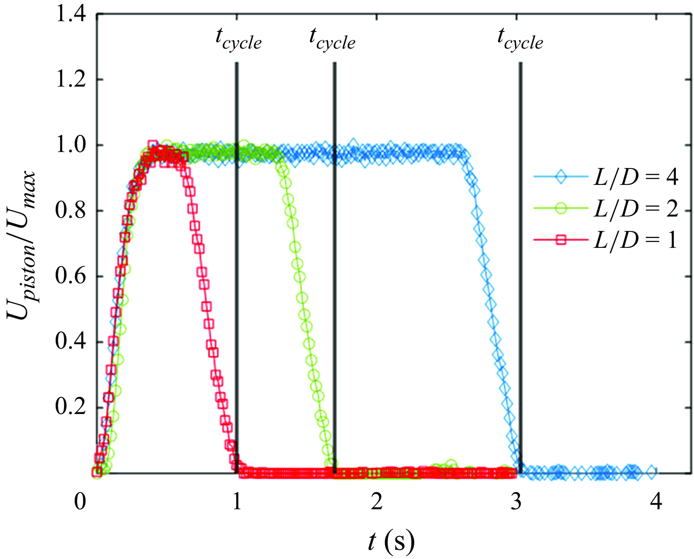
Figure 2. Measured syringe pump piston velocity by syringe motion normalised by the programmed maximum velocity for the pump ( $U_{max}$
).
$U_{max}$
).
2.2. Nozzle construction and characterisation
A rigid nozzle was 3D printed out of PLA plastic with a layer height of 0.03 mm. The rigid nozzle was manufactured to be the same length ( $L_{nozzle}=11.5$
cm) as the flexible nozzles, with the only difference being a bevelled edge of 25 degrees at the exit. This nozzle design was selected to be consistent with previous studies in vortex ring literature (Gharib et al. Reference Gharib, Rambod and Shariff1998; Krueger & Gharib Reference Krueger and Gharib2003; Dabiri & Gharib Reference Dabiri and Gharib2005).
$L_{nozzle}=11.5$
cm) as the flexible nozzles, with the only difference being a bevelled edge of 25 degrees at the exit. This nozzle design was selected to be consistent with previous studies in vortex ring literature (Gharib et al. Reference Gharib, Rambod and Shariff1998; Krueger & Gharib Reference Krueger and Gharib2003; Dabiri & Gharib Reference Dabiri and Gharib2005).
The flexible nozzles were moulded from SmoothOn SortaClear 40A two-part liquid silicone. The selected nozzle construction method was adopted from Choi & Park (Reference Choi and Park2022), using a pour mould method over a 2.55 cm diameter ( $D$
) aluminium rod press fit into a 3D printed base to create the mounting surface for the flexible nozzles. Figure 1 shows a complete flexible nozzle with the integrated mounting surface, and figure 3(a) shows an isometric view of the flexible nozzle geometry. After curing, the nozzles were cut to a length (
$D$
) aluminium rod press fit into a 3D printed base to create the mounting surface for the flexible nozzles. Figure 1 shows a complete flexible nozzle with the integrated mounting surface, and figure 3(a) shows an isometric view of the flexible nozzle geometry. After curing, the nozzles were cut to a length ( $L_{nozzle}$
) of 11.5 cm measured from the top of the nozzle base to the edge of the nozzle exit, resulting in an aspect ratio (
$L_{nozzle}$
) of 11.5 cm measured from the top of the nozzle base to the edge of the nozzle exit, resulting in an aspect ratio ( ${L_{nozzle}}/{D}$
) of 4.55. This aspect ratio was chosen to ensure all of the fluid ejected was initially contained within the nozzle. This is in contrast to Choi & Park (Reference Choi and Park2022, Reference Choi and Park2024), where a aspect ratio of 2 was used (ejected fluid slug not initially fully contained within flexible nozzle). The stiffness of the flexible nozzles was controlled by adding different mass percentages (
${L_{nozzle}}/{D}$
) of 4.55. This aspect ratio was chosen to ensure all of the fluid ejected was initially contained within the nozzle. This is in contrast to Choi & Park (Reference Choi and Park2022, Reference Choi and Park2024), where a aspect ratio of 2 was used (ejected fluid slug not initially fully contained within flexible nozzle). The stiffness of the flexible nozzles was controlled by adding different mass percentages ( $\%ma = 15\,\% - 50\,\%$
) of SmoothOn silicone thinner relative to the base liquid silicone mixture.
$\%ma = 15\,\% - 50\,\%$
) of SmoothOn silicone thinner relative to the base liquid silicone mixture.
The flexible nozzles were mounted to the experimental set-up using a 3D printed part that clamped onto the base of the nozzle using bolts, shown in figure 1. This set-up was used to reduce stress concentrations from forming at the edges of the nozzle which could potentially affect the nozzle deformation behaviour. Additionally, the mount created a consistent rigid boundary condition between the different nozzles to ensure repeatability of the experiment. After a nozzle was clamped onto the mount, it was installed onto the outlet pipe using an interference fit. The rigid nozzle was similarly installed with an interference fit on the outlet pipe.
For each nozzle, a representative nozzle was made to be sliced into strips to measure the mean nozzle wall thickness ( $h$
) using an Olympus BX60 microscope with a 10
$h$
) using an Olympus BX60 microscope with a 10 $\,\times\,$
power lens. The wall thickness was measured at a total of 16 locations for each nozzle, at 4 streamwise locations 2.5 cm apart and 4 equally spaced azimuthal locations around the nozzle circumference at each streamwise height as shown in figure 3(a). The wall thickness variation was negligible with a maximum azimuthal variation of 4.1 % for the manufactured nozzles. The wall thickness varied approximately linearly along each nozzle’s length due to the pour moulding manufacturing method. The spatial distribution of the wall thickness along the nozzle length (
$\,\times\,$
power lens. The wall thickness was measured at a total of 16 locations for each nozzle, at 4 streamwise locations 2.5 cm apart and 4 equally spaced azimuthal locations around the nozzle circumference at each streamwise height as shown in figure 3(a). The wall thickness variation was negligible with a maximum azimuthal variation of 4.1 % for the manufactured nozzles. The wall thickness varied approximately linearly along each nozzle’s length due to the pour moulding manufacturing method. The spatial distribution of the wall thickness along the nozzle length ( $L$
) is plotted in figure 3(b). The thickness decreased at an average rate of 17.7 µm/
$L$
) is plotted in figure 3(b). The thickness decreased at an average rate of 17.7 µm/ $D^{-1}$
along the streamwise direction of the nozzle. The total change in thickness was approximately constant between the different nozzles, thus the thickness was averaged over the measured locations for each nozzle. Mean wall thickness (
$D^{-1}$
along the streamwise direction of the nozzle. The total change in thickness was approximately constant between the different nozzles, thus the thickness was averaged over the measured locations for each nozzle. Mean wall thickness ( $h$
) varied from 188.4 to 96.8 µm across the different nozzles, and the nozzle inner diameter was held constant.
$h$
) varied from 188.4 to 96.8 µm across the different nozzles, and the nozzle inner diameter was held constant.
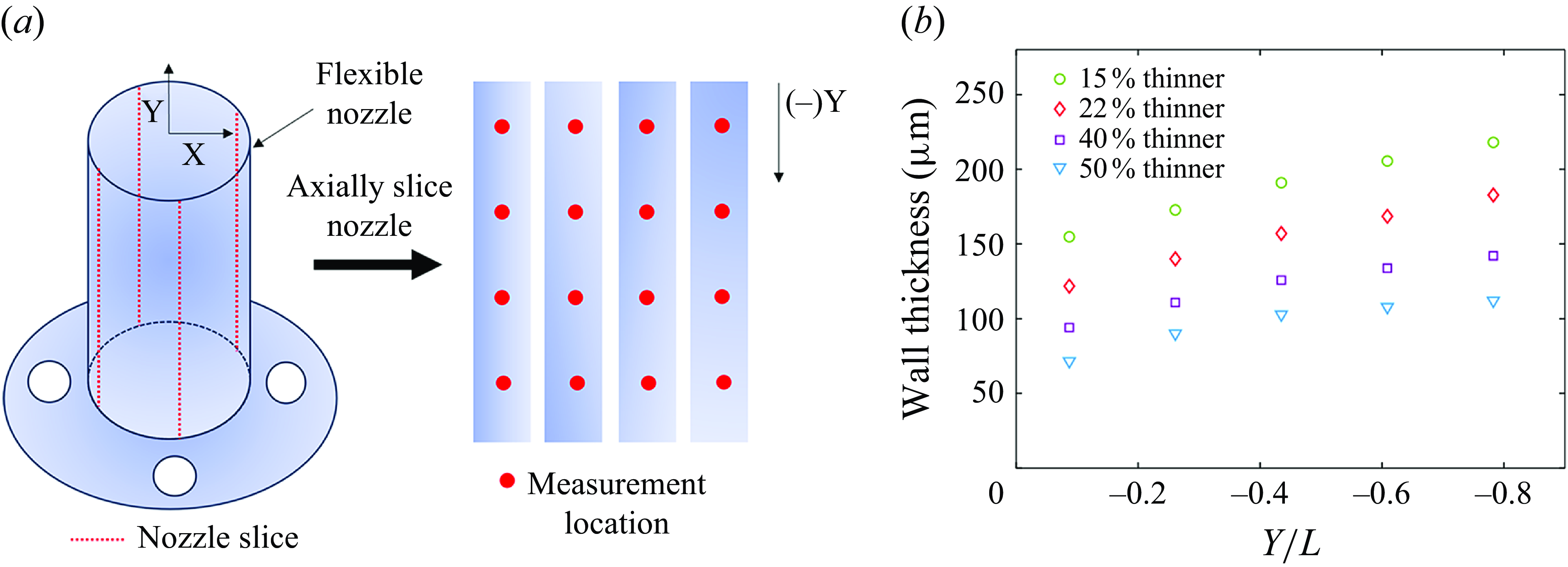
Figure 3. Nozzle wall thickness measurement schematic and variation in wall thickness. (a) Schematic indicating the cut sections used for measuring nozzle wall thickness. The nozzles were cut along their streamwise direction to create 4 strips that were measured at 4 streamwise locations along the nozzle’s length. (b) Distribution of measured nozzle thickness along the length ( $L$
) of the nozzles. The labelled per cent values in the legend correspond to the %ma of silicone thinner added to the mixture to mould each nozzle.
$L$
) of the nozzles. The labelled per cent values in the legend correspond to the %ma of silicone thinner added to the mixture to mould each nozzle.
Young’s modulus was calculated by completing tensile tests on 5 mm thick dog bone samples prepared with cross-sectional geometry as described in ASTM D412-16 standard test methods for vulcanised rubber and thermoplastic elastomers – tension (AST 2021). The tests were completed on an Instron 312 series frame with a 25 kN load cell. For each nozzle, 8 tensile tests were completed from two different batches of silicone, one batch from the silicone used for the experimental nozzle, and second batch from the silicone used for the representative nozzle. The maximum variation in $E$
between the two sets was negligible, with the maximum being 4.2 %. Young’s modulus (
$E$
between the two sets was negligible, with the maximum being 4.2 %. Young’s modulus ( $E$
) varied from 404 to 193 kPa, as shown in figure 4(a).
$E$
) varied from 404 to 193 kPa, as shown in figure 4(a).
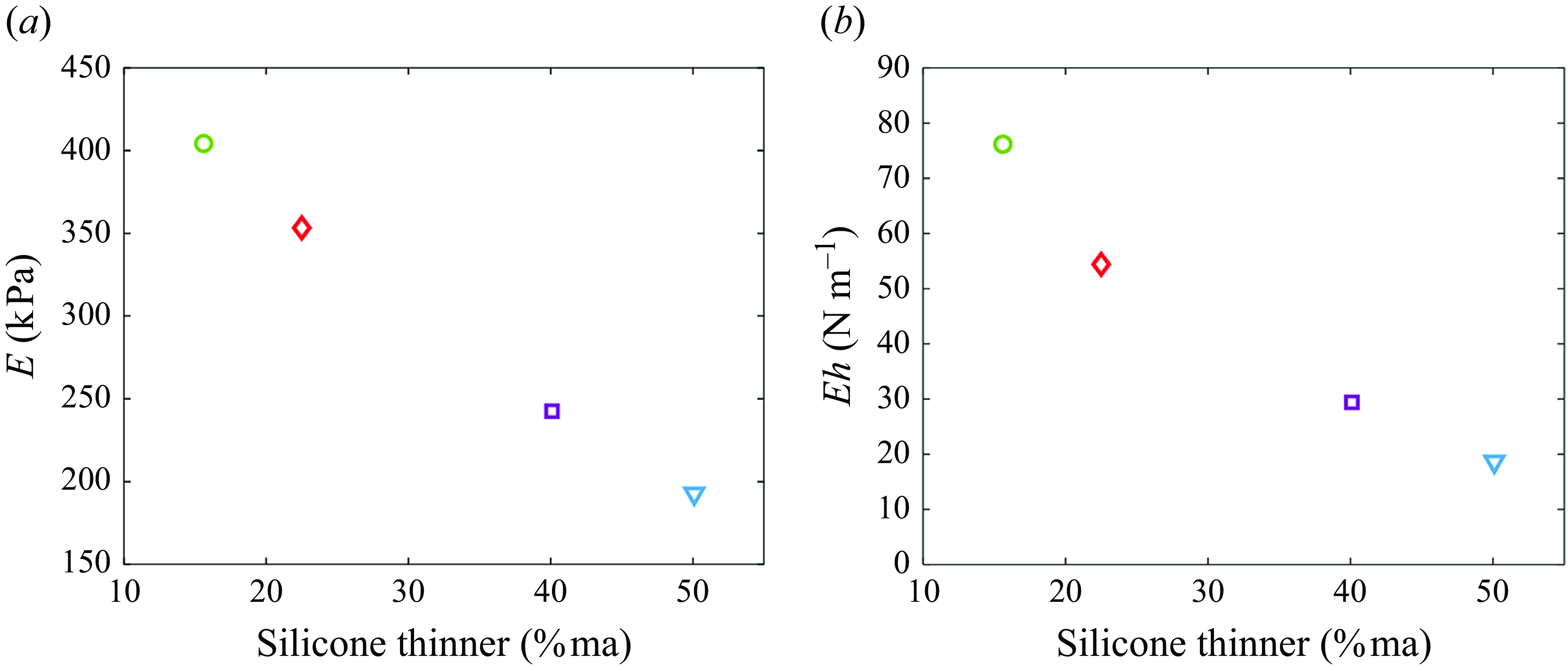
Figure 4. Material properties measured with varied %ma thinner (a) Young’s modulus ( $E$
) averaged over 8 samples from each %ma of silicone thinner added to the nozzle mixtures. (b) Value of
$E$
) averaged over 8 samples from each %ma of silicone thinner added to the nozzle mixtures. (b) Value of $E$
multiplied by the mean wall thickness (
$E$
multiplied by the mean wall thickness ( $h$
), defining the characteristic stiffness of the varied %ma thinner nozzles.
$h$
), defining the characteristic stiffness of the varied %ma thinner nozzles.
The representative characteristic stiffness parameter was chosen to be Young’s modulus ( $E$
) multiplied by the mean wall thickness (
$E$
) multiplied by the mean wall thickness ( $h$
), which is plotted in figure 4(b). Overall, a set of 5 nozzles were tested with characteristic stiffness parameter
$h$
), which is plotted in figure 4(b). Overall, a set of 5 nozzles were tested with characteristic stiffness parameter $Eh$
= 19, 29, 54, 78 and
$Eh$
= 19, 29, 54, 78 and $Eh = \infty\,\rm N\, m^-{^1}$
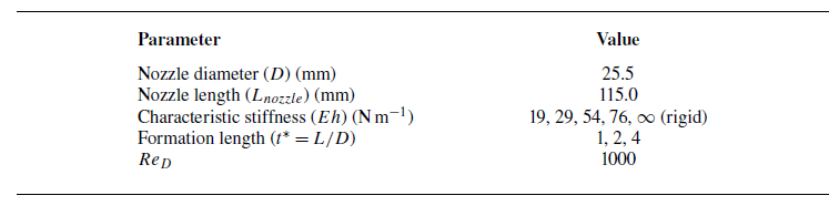
(rigid). Table 1 summarises the parameters studied in this experiment.
$Eh = \infty\,\rm N\, m^-{^1}$
(rigid). Table 1 summarises the parameters studied in this experiment.
Table 1. Experimental parameters.
2.3. Velocity field measurements
Particle image velocimetry (PIV) was conducted to quantify the velocity vector fields beneath the nozzles. Images were sampled at 60 Hz with a resolution of 1080 $\,\times\,$
1920 pixels. A total of 600 image pairs were analysed for each experimental run. The camera was triggered to start simultaneously with the initiation of the pump using an in-house LabVIEW program via a MyDAQ (National Instruments). Hollow glass sphere particles with mean diameter of 10 µm, and average density of 1.10 g ml−1 were used to seed the tank (Potters’ Industries Sphericel, 110P8). A 532 nm continuous wavelength laser and a convex cylindrical lens were mounted underneath the tank to illuminate a 1 mm vertical sheet passing through the centre cross-section of the nozzle in either the XY or XZ plane as defined in figure 1, with the Z direction being out of the page. Cross-correlation of the image pairs was completed using a multiple pass interrogation method with successive reductions in window sizes using the open-source software PIVlab (Thielicke & Sonntag 2021; Thielicke Reference Thielicke2022). For a field of view of 5.5
$\,\times\,$
1920 pixels. A total of 600 image pairs were analysed for each experimental run. The camera was triggered to start simultaneously with the initiation of the pump using an in-house LabVIEW program via a MyDAQ (National Instruments). Hollow glass sphere particles with mean diameter of 10 µm, and average density of 1.10 g ml−1 were used to seed the tank (Potters’ Industries Sphericel, 110P8). A 532 nm continuous wavelength laser and a convex cylindrical lens were mounted underneath the tank to illuminate a 1 mm vertical sheet passing through the centre cross-section of the nozzle in either the XY or XZ plane as defined in figure 1, with the Z direction being out of the page. Cross-correlation of the image pairs was completed using a multiple pass interrogation method with successive reductions in window sizes using the open-source software PIVlab (Thielicke & Sonntag 2021; Thielicke Reference Thielicke2022). For a field of view of 5.5 $D$
$D$ $\times$
3
$\times$
3 $D$
, a final interrogation window size of 64
$D$
, a final interrogation window size of 64 $\,\times\,$
64 pixels with 50 % overlap was chosen. This resulted in a vector space of 59
$\,\times\,$
64 pixels with 50 % overlap was chosen. This resulted in a vector space of 59 $\,\times\,$
32 vectors with a vector spacing of 0.098
$\,\times\,$
32 vectors with a vector spacing of 0.098 $D$
. The time interval between image pairs,
$D$
. The time interval between image pairs, $\Delta t$
, was 0.0167 s and the particle motion between image pairs was limited to approximately 1/4 of the window size to ensure the accuracy of the cross-correlation (Willert & Gharib Reference Willert and Gharib1991). As the flexible nozzles were found to deform about a preferential axis, PIV was performed both perpendicular (XY plane), and parallel (XZ plane), to this preferential axis to ensure axisymmetry in our results (see Appendix A for further details). For each nozzle, 10 trials were completed, with 5 trials from each plane. In subsequent plots, the average of these 10 trials is plotted unless otherwise noted. The mean maximum spatially averaged velocity measured
$\Delta t$
, was 0.0167 s and the particle motion between image pairs was limited to approximately 1/4 of the window size to ensure the accuracy of the cross-correlation (Willert & Gharib Reference Willert and Gharib1991). As the flexible nozzles were found to deform about a preferential axis, PIV was performed both perpendicular (XY plane), and parallel (XZ plane), to this preferential axis to ensure axisymmetry in our results (see Appendix A for further details). For each nozzle, 10 trials were completed, with 5 trials from each plane. In subsequent plots, the average of these 10 trials is plotted unless otherwise noted. The mean maximum spatially averaged velocity measured $0.019D$
below the rigid nozzle outlet was calculated to be 3.97 cm s−1 across all ejected volumes, with a 95 % confidence interval of
$0.019D$
below the rigid nozzle outlet was calculated to be 3.97 cm s−1 across all ejected volumes, with a 95 % confidence interval of $\pm$
0.1 cm s−1 based on a one sample t test. All reported confidence intervals hereon represent the 95 % confidence interval based on a one sample t test. The flexible nozzles altered the measured exit velocity, which is discussed in § 3, where the
$\pm$
0.1 cm s−1 based on a one sample t test. All reported confidence intervals hereon represent the 95 % confidence interval based on a one sample t test. The flexible nozzles altered the measured exit velocity, which is discussed in § 3, where the $Eh = 29\,\rm N\,m^-{^1}$
nozzle had the largest variation, with mean maximum spatial averaged velocity of 6.40 cm s−1 and confidence interval
$Eh = 29\,\rm N\,m^-{^1}$
nozzle had the largest variation, with mean maximum spatial averaged velocity of 6.40 cm s−1 and confidence interval $\pm$
0.3 cm s−1.
$\pm$
0.3 cm s−1.
2.4. Nozzle deformation measurements
To track the side deformation of the flexible nozzles, the particles were removed from the tank, and the laser sheet was used to illuminate the longitudinal centre cross-section of the nozzle in the XY and XZ planes. The camera imaged the centre plane deformations, which were used for nozzle tracking with an in-house MATLAB edge detection code. The same image processing steps were applied to these images as was used to determine the syringe pump velocity profiles. Two time sets were considered, forced vibration when the pump was active, and free vibration when the pump had stopped moving and the nozzle was freely oscillating. The bottom millimetre of the nozzle was used as a representative point to track the position over time. Fast Fourier transforms (FFTs) were completed in MATLAB to find the repeated oscillations frequencies from the free vibration positional datasets. The single-side amplitude spectrum of the position data, or the occurrence of each frequency in the positive domain, was calculated using a sampling period of 0.0167 sec and sample length of 600 samples (10 s). The single sided amplitude spectrum was plotted to find a peak in frequency occurrences to estimate the damped natural frequency of ( $\omega _{d}$
) of the nozzles. The deformation viewed from beneath the nozzle (YZ plane) was also imaged.
$\omega _{d}$
) of the nozzles. The deformation viewed from beneath the nozzle (YZ plane) was also imaged.
2.5. FTLE fields and ridges
The predicted material boundaries of the generated vortex rings were identified by detecting ridges within the FTLE field using the LCS Matlab Kit V2 by the Biological Propulsion Laboratory at the California Institute of Technology (Shadden et al. Reference Shadden, Dabiri and Marsden2006; Peng & Dabiri Reference Peng and Dabiri2009; Dabiri Reference Dabiri2021). The FTLE fields are directly derived from the velocity fields generated from PIV by either initiating fluid particle tracking forward or backward in time. This process yields both positive (forward) pFTLE and negative (backward) nFTLE fields. The FTLE field is computed by
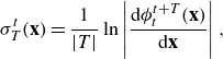 \begin{equation} \sigma _{T}^{t}(\mathbf{x}) = \frac {1}{|T|} \ln \left | \frac {{\rm d}\phi ^{t+T}_{t}(\mathbf{x})}{{\rm d}\mathbf{x}} \right |, \end{equation}
where $ \sigma _{T}^{t}(\mathbf{x})$
represents the scalar FTLE field, or how much particles nearby a point diverge, and
$ \sigma _{T}^{t}(\mathbf{x})$
represents the scalar FTLE field, or how much particles nearby a point diverge, and $\phi^{t+T}_{t}(\mathbf{x})$
signifies the flow map of particles from their location at signifies the flow map of particles from their location at
$\phi^{t+T}_{t}(\mathbf{x})$
signifies the flow map of particles from their location at signifies the flow map of particles from their location at $\mathbf{x}$
at time
$\mathbf{x}$
at time $t$
to
$t$
to $t+T$
and
$t+T$
and $|T|$
represents the integration time used to track the particle motion, with
$|T|$
represents the integration time used to track the particle motion, with $T\lt 0$
, indicating backward time and
$T\lt 0$
, indicating backward time and $T\gt 0$
, corresponding to forward time. After obtaining the FTLE fields, regions of local maxima, or ridges, were identified to pinpoint regions where fluid transport is restricted or intensified. These ridges are known as Lagrangian coherent structures (LCS), which are valuable for analysing vortex ring pinch-off. Negative LCS (nLCS), found from the ridges within a nFTLE field, indicate an attractive material lines in the flow field, while positive LCS (pLCS), found from ridges within a pFTLE field, indicate repelling material lines. When a nLCS and pLCS combine to form a closed loop, it signifies the formation of a pinched-off vortex ring (Shadden et al. Reference Shadden, Dabiri and Marsden2006). The presence of a pLCS on a vortex ring’s rear edge suggests that further fluid entry into the enclosed structure of the vortex ring from the vortex generator is unlikely, and the vortex ring will not gain additional vorticity. The integration length
$T\gt 0$
, corresponding to forward time. After obtaining the FTLE fields, regions of local maxima, or ridges, were identified to pinpoint regions where fluid transport is restricted or intensified. These ridges are known as Lagrangian coherent structures (LCS), which are valuable for analysing vortex ring pinch-off. Negative LCS (nLCS), found from the ridges within a nFTLE field, indicate an attractive material lines in the flow field, while positive LCS (pLCS), found from ridges within a pFTLE field, indicate repelling material lines. When a nLCS and pLCS combine to form a closed loop, it signifies the formation of a pinched-off vortex ring (Shadden et al. Reference Shadden, Dabiri and Marsden2006). The presence of a pLCS on a vortex ring’s rear edge suggests that further fluid entry into the enclosed structure of the vortex ring from the vortex generator is unlikely, and the vortex ring will not gain additional vorticity. The integration length $|T|$
chosen for the data analysed within this paper corresponds to 1 s, or 60 image frames. A step size of 1 and time step of 0.0167 s per frame were used.
$|T|$
chosen for the data analysed within this paper corresponds to 1 s, or 60 image frames. A step size of 1 and time step of 0.0167 s per frame were used.
3. Results and discussion
3.1. Changes in flow characteristics due to nozzle flexibility
First, we examine how the development of the vortical structures in the flow fields is influenced by the fluid structure interaction as the characteristic stiffness parameter ( $Eh$
) is varied for the given input flow parameters. Figure 5(a) illustrates the flow development from the
$Eh$
) is varied for the given input flow parameters. Figure 5(a) illustrates the flow development from the $Eh = \infty\,\rm N\,m^-{^1}$
(rigid) nozzle for
$Eh = \infty\,\rm N\,m^-{^1}$
(rigid) nozzle for ${L}/{D}=2$
from (i)
${L}/{D}=2$
from (i) $t/t_{cycle}=0.41$
to (iv)
$t/t_{cycle}=0.41$
to (iv) $t/t_{cycle}=3$
, where
$t/t_{cycle}=3$
, where $t_{cycle}$
is the time when the pump stops for each
$t_{cycle}$
is the time when the pump stops for each ${L}/{D}$
. The nozzle position relative to the flow field is shown as the black trapezoid at the top of each frame. As the fluid is expelled from the nozzle, the shear layer rolls up, forming a single primary vortex (PV) ring as it enters the quiescent tank. The plots show a cross-section cut across the middle of the ring, which is displayed as a single counter rotating vortex pair of opposite sign vorticity. This is consistent with Gharib et al. (Reference Gharib, Rambod and Shariff1998), wherein the ejected fluid from impulsive piston motion will form a single vortex ring for
${L}/{D}$
. The nozzle position relative to the flow field is shown as the black trapezoid at the top of each frame. As the fluid is expelled from the nozzle, the shear layer rolls up, forming a single primary vortex (PV) ring as it enters the quiescent tank. The plots show a cross-section cut across the middle of the ring, which is displayed as a single counter rotating vortex pair of opposite sign vorticity. This is consistent with Gharib et al. (Reference Gharib, Rambod and Shariff1998), wherein the ejected fluid from impulsive piston motion will form a single vortex ring for ${L}/{D} \lt 4$
. However, this behaviour changes when
${L}/{D} \lt 4$
. However, this behaviour changes when $Eh$
is sufficiently low enough (flexible enough) to perturb the input flow conditions.
$Eh$
is sufficiently low enough (flexible enough) to perturb the input flow conditions.
Figure 5(b–e; i – iv) shows the flexible nozzle ( $Eh$
= 76, 54, 29, 19 N m–1) flow fields, under the same input kinematic flow conditions from the pump (
$Eh$
= 76, 54, 29, 19 N m–1) flow fields, under the same input kinematic flow conditions from the pump ( ${L}/{D} \lt 2$
). As
${L}/{D} \lt 2$
). As $Eh$
decreases (becomes more flexible) the flow structures begin to deviate from the rigid case. For
$Eh$
decreases (becomes more flexible) the flow structures begin to deviate from the rigid case. For $Eh = 76\,\rm N\,m^-{^1}$
the vortex cores are slightly elongated, but become approximately circular after
$Eh = 76\,\rm N\,m^-{^1}$
the vortex cores are slightly elongated, but become approximately circular after $t/t_{cycle}$
= 1. It is understood that the alteration is due to small-scale oscillations (
$t/t_{cycle}$
= 1. It is understood that the alteration is due to small-scale oscillations ( $\approx {0.02D}$
) of the flexible nozzle. As
$\approx {0.02D}$
) of the flexible nozzle. As $Eh$
is lowered further, the deformation of the nozzles becomes an order of magnitude more pronounced (up to
$Eh$
is lowered further, the deformation of the nozzles becomes an order of magnitude more pronounced (up to $\approx {0.19D}$
), multiple distinct vortex structures form, and the PV begins to significantly differ from the rigid case. For
$\approx {0.19D}$
), multiple distinct vortex structures form, and the PV begins to significantly differ from the rigid case. For $Eh = 54\,\rm N\,m^-{^1}$
in figure 5(c), two cores form, where the secondary vorticity eventually leap frogs through the PV core, but the two cores do not separate from one another. The formation of this second core of vorticity corresponds to the nozzle oscillations and rapid collapse at
$Eh = 54\,\rm N\,m^-{^1}$
in figure 5(c), two cores form, where the secondary vorticity eventually leap frogs through the PV core, but the two cores do not separate from one another. The formation of this second core of vorticity corresponds to the nozzle oscillations and rapid collapse at $t=t_{cycle}$
, which is examined further below. For
$t=t_{cycle}$
, which is examined further below. For $Eh = 29\,\rm N\,m^-{^1}$
in figure 5(d), the PV separates from the nozzle prior to
$Eh = 29\,\rm N\,m^-{^1}$
in figure 5(d), the PV separates from the nozzle prior to $t/t_{cycle} = 1$
. A weak secondary vortex (SV) structure forms, and separates from the nozzle at
$t/t_{cycle} = 1$
. A weak secondary vortex (SV) structure forms, and separates from the nozzle at $t/t_{cycle}$
= 2. Notably the PV travels significantly further than the rigid case reaching
$t/t_{cycle}$
= 2. Notably the PV travels significantly further than the rigid case reaching $2.8D$
compared with
$2.8D$
compared with $1.6D$
at
$1.6D$
at $t/t_{cycle} = 2$
, defined by the averaged location of peak vorticity between the positive and negative cores. For the most flexible nozzle,
$t/t_{cycle} = 2$
, defined by the averaged location of peak vorticity between the positive and negative cores. For the most flexible nozzle, $Eh = 19\,\rm N\,m^-{^1}$
, two separate vortex structures also form, but the SV is slightly larger than that produced by the
$Eh = 19\,\rm N\,m^-{^1}$
, two separate vortex structures also form, but the SV is slightly larger than that produced by the $Eh = 29\,\rm N\,m^-{^1}$
nozzle. Interestingly, in this case, the PV travels a shorter distance of
$Eh = 29\,\rm N\,m^-{^1}$
nozzle. Interestingly, in this case, the PV travels a shorter distance of $2.4D$
below the nozzle at
$2.4D$
below the nozzle at $t/t_{cycle} = 2$
compared with the slightly stiffer
$t/t_{cycle} = 2$
compared with the slightly stiffer $Eh = 29\,\rm N\,m^-{^1}$
nozzle. Similar trends are observed at the other ejected volumes (
$Eh = 29\,\rm N\,m^-{^1}$
nozzle. Similar trends are observed at the other ejected volumes ( ${L}/{D} = 1, 4$
), see Supplementary Material 1.
${L}/{D} = 1, 4$
), see Supplementary Material 1.
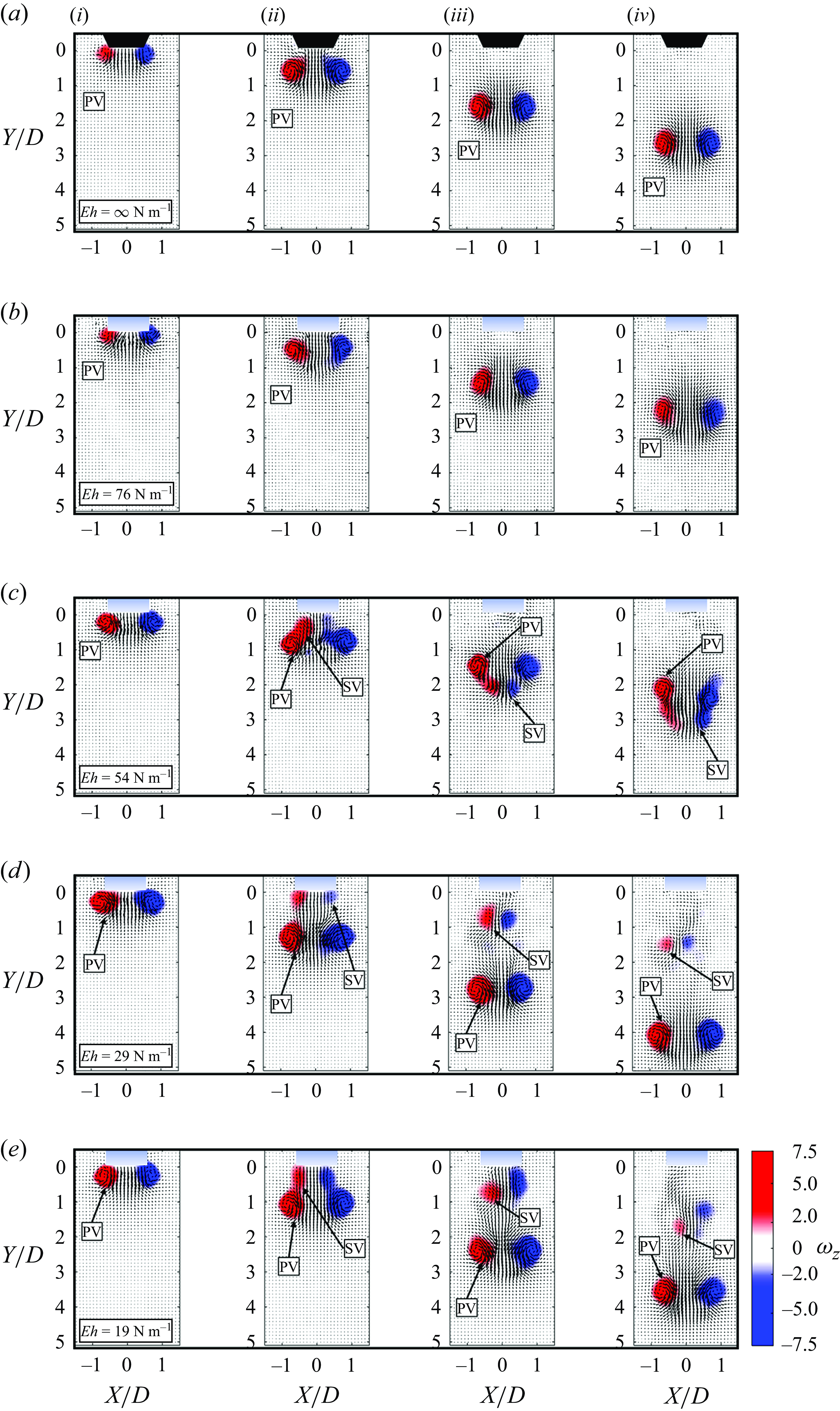
Figure 5. Vorticity and vector fields measured for (i) $t/t_{cycle}=0.41$
, (ii)
$t/t_{cycle}=0.41$
, (ii) $t/t_{cycle}=1$
, (iii)
$t/t_{cycle}=1$
, (iii) $t/t_{cycle}=2$
and (iv)
$t/t_{cycle}=2$
and (iv) $t/t_{cycle}=3$
for each nozzle given the same kinematic input from the pump for
$t/t_{cycle}=3$
for each nozzle given the same kinematic input from the pump for ${L}/{D} = 2$
. (a) Rigid nozzle (
${L}/{D} = 2$
. (a) Rigid nozzle ( $Eh = \infty\,\rm N\,m^-{^1}$
); (b)
$Eh = \infty\,\rm N\,m^-{^1}$
); (b) $Eh=76\,\rm N\,m^-{^1}$
; (c)
$Eh=76\,\rm N\,m^-{^1}$
; (c) $Eh=54\,\rm N\,m^-{^1}$
; (d)
$Eh=54\,\rm N\,m^-{^1}$
; (d) $Eh= 29\,\rm N\,m^-{^1}$
; (e)
$Eh= 29\,\rm N\,m^-{^1}$
; (e) $Eh=19\,\rm N\,m^-{^1}$
.
$Eh=19\,\rm N\,m^-{^1}$
.
To compare between the vortex rings produced by the different nozzles, we analyse cross-sectional cuts of the vortex rings generated by the $Eh = \infty\,\rm N\,m^-{^1}$
(rigid) nozzle and the
$Eh = \infty\,\rm N\,m^-{^1}$
(rigid) nozzle and the $Eh = 29\,\rm N\,m^-{^1}$
nozzle, at
$Eh = 29\,\rm N\,m^-{^1}$
nozzle, at $t/t_{cycle}=2$
for
$t/t_{cycle}=2$
for ${L}/{D}=1$
. This simplifies the comparison by focusing on single PV structures as shown in the vorticity plots in figures 6(a) and 6(b). Figures 6(c) and 6(d) display the spatial distribution of vorticity and velocity components measured along the cut lines. These cut lines are defined by the vertical (
${L}/{D}=1$
. This simplifies the comparison by focusing on single PV structures as shown in the vorticity plots in figures 6(a) and 6(b). Figures 6(c) and 6(d) display the spatial distribution of vorticity and velocity components measured along the cut lines. These cut lines are defined by the vertical ( $Y$
) location of peak vorticity for each trial. As inferred by the distance travelled by the PV produced from the
$Y$
) location of peak vorticity for each trial. As inferred by the distance travelled by the PV produced from the $Eh = 29\,\rm N\,m^-{^1}$
nozzle, the peak velocity is 2.5 times higher, and the peak vorticity is 2.8 times higher than the rigid nozzle case. Additionally, the wider spatial distribution velocity and vorticity suggests that the
$Eh = 29\,\rm N\,m^-{^1}$
nozzle, the peak velocity is 2.5 times higher, and the peak vorticity is 2.8 times higher than the rigid nozzle case. Additionally, the wider spatial distribution velocity and vorticity suggests that the $Eh = 29\,\rm N\,m^-{^1}$
nozzle not only produces a stronger PV, but a larger PV compared with the rigid nozzle.
$Eh = 29\,\rm N\,m^-{^1}$
nozzle not only produces a stronger PV, but a larger PV compared with the rigid nozzle.
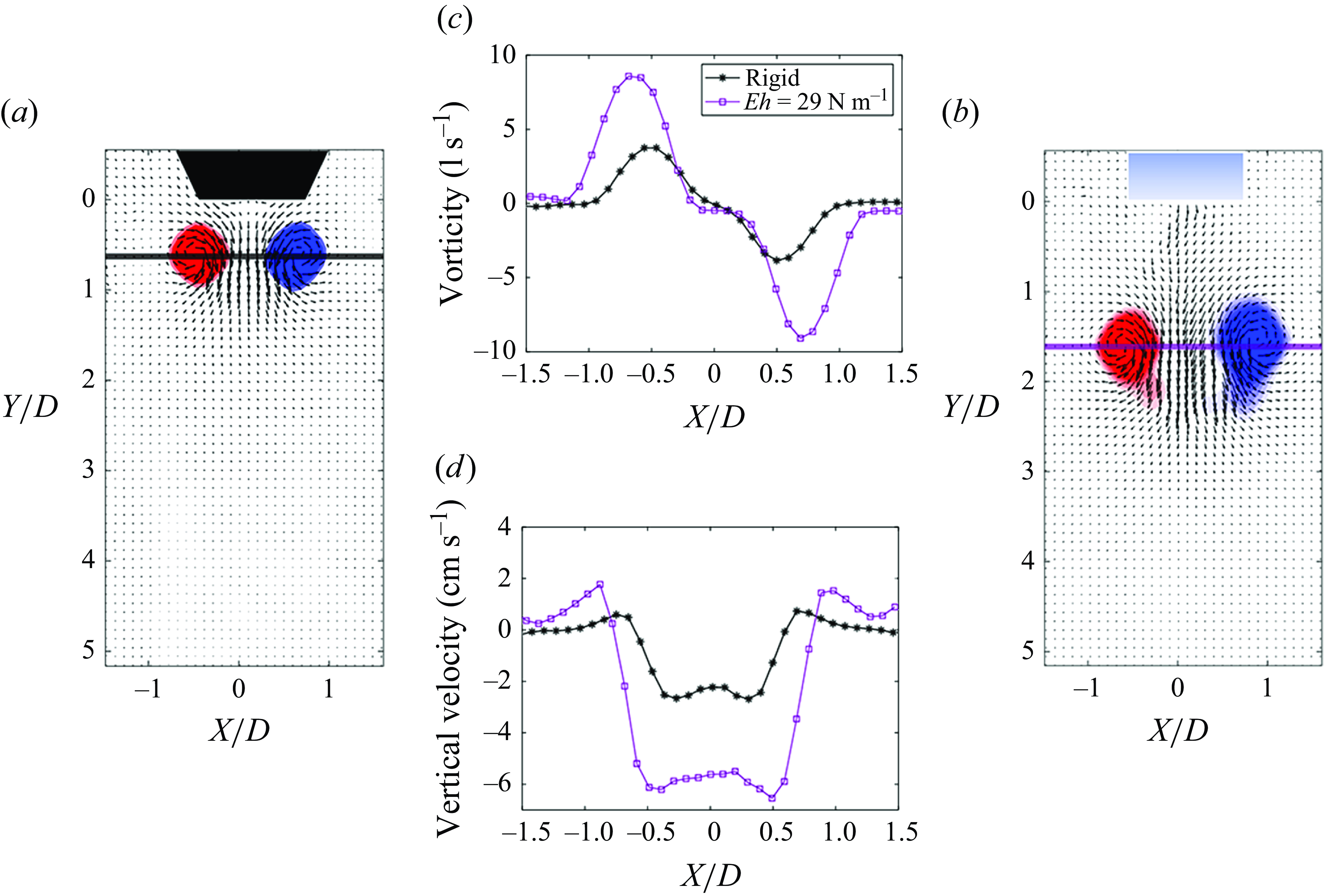
Figure 6. (a) Rigid nozzle PIV vector plot and vorticity at $t/t_{cycle}=2$
for
$t/t_{cycle}=2$
for ${L}/{D}=1$
. The solid line represents a cut section of the vortex ring and corresponds to the centred plots of vorticity and velocity; (b)
${L}/{D}=1$
. The solid line represents a cut section of the vortex ring and corresponds to the centred plots of vorticity and velocity; (b) $Eh = 29\,\rm N\,m^-{^1}$
nozzle PIV vector plot and vorticity, with cut line selected by the point of highest vorticity. (c) Vorticity across the vortex ring cut plane for the rigid and
$Eh = 29\,\rm N\,m^-{^1}$
nozzle PIV vector plot and vorticity, with cut line selected by the point of highest vorticity. (c) Vorticity across the vortex ring cut plane for the rigid and $Eh = 29\,\rm N\,m^-{^1}$
nozzles. (d) Vertical velocity across the vortex ring cut plane for the rigid and
$Eh = 29\,\rm N\,m^-{^1}$
nozzles. (d) Vertical velocity across the vortex ring cut plane for the rigid and $Eh = 29\,\rm N\,m^-{^1}$
nozzles. Legend is the same for (c) and (d).
$Eh = 29\,\rm N\,m^-{^1}$
nozzles. Legend is the same for (c) and (d).
Next we analyse the temporal variation of vortex spacing ( $b$
) and core diameter (
$b$
) and core diameter ( $a$
) for each nozzle, as plotted in figures 7(a) and 7(b) for
$a$
) for each nozzle, as plotted in figures 7(a) and 7(b) for ${L}/{D}=2$
. The PV ring is tracked for this analysis, with
${L}/{D}=2$
. The PV ring is tracked for this analysis, with $b$
defined as the distance between the peak vorticity values of each core, and
$b$
defined as the distance between the peak vorticity values of each core, and $a$
is defined by the distance between the two points bounding 10 % of the maximum vorticity, averaged between the positive and negative cores. As shown in figure 7(a), the flexible nozzles generate vortex rings with wider spacing, with each ring converging to an approximately constant spacing of
$a$
is defined by the distance between the two points bounding 10 % of the maximum vorticity, averaged between the positive and negative cores. As shown in figure 7(a), the flexible nozzles generate vortex rings with wider spacing, with each ring converging to an approximately constant spacing of ${b}/{D} = 1.41 \pm 0.15$
, compared with
${b}/{D} = 1.41 \pm 0.15$
, compared with ${b}/{D} = 1.19 \pm 0.13$
for the
${b}/{D} = 1.19 \pm 0.13$
for the $Eh = \infty\,\rm N\,m^-{^1}$
(rigid) nozzle at
$Eh = \infty\,\rm N\,m^-{^1}$
(rigid) nozzle at $t=3t_{cycle}$
. The vortex ring core diameter (
$t=3t_{cycle}$
. The vortex ring core diameter ( $a$
) varies slightly with
$a$
) varies slightly with $Eh$
, with the flexible nozzles all creating larger cores, as shown in figure 7(b). The
$Eh$
, with the flexible nozzles all creating larger cores, as shown in figure 7(b). The $Eh = 54$
,
$Eh = 54$
, $29$
and
$29$
and $19\,\rm N\,m^-{^1}$
nozzles converge to a core diameter of
$19\,\rm N\,m^-{^1}$
nozzles converge to a core diameter of ${a}/{D} = 1.13 \pm 0.09$
, and the
${a}/{D} = 1.13 \pm 0.09$
, and the $Eh = 76\,\rm N\,m^-{^1}$
nozzle converges to
$Eh = 76\,\rm N\,m^-{^1}$
nozzle converges to ${a}/{D} = 1.01 \pm 0.09$
, compared with
${a}/{D} = 1.01 \pm 0.09$
, compared with ${a}/{D} = 0.82 \pm 0.06$
for
${a}/{D} = 0.82 \pm 0.06$
for $Eh = \infty\,\rm N\,m^-{^1}$
at
$Eh = \infty\,\rm N\,m^-{^1}$
at $t=3t_{cycle}$
. Here, the bounds are defined by the 95 % confidence interval for
$t=3t_{cycle}$
. Here, the bounds are defined by the 95 % confidence interval for ${L}/{D} = 2$
. The other ejected volumes follow the same trends, but with smaller core diameter and spacing for
${L}/{D} = 2$
. The other ejected volumes follow the same trends, but with smaller core diameter and spacing for ${L}/{D} = 1$
, and larger for
${L}/{D} = 1$
, and larger for ${L}/{D} = 4$
. Given the larger (
${L}/{D} = 4$
. Given the larger ( $b, a$
), stronger (
$b, a$
), stronger ( $\omega _z$
), and faster moving vortex rings generated by the flexible nozzles, the velocity produced by these nozzles should scale accordingly.
$\omega _z$
), and faster moving vortex rings generated by the flexible nozzles, the velocity produced by these nozzles should scale accordingly.

Figure 7. Primary vortex ring spatial parameters measured for ${L}/{D}=2$
. Points are plotted every 0.083 sec for clarity. (a) Vortex spacing (
${L}/{D}=2$
. Points are plotted every 0.083 sec for clarity. (a) Vortex spacing ( $b$
), normalised by the nozzle diameter (
$b$
), normalised by the nozzle diameter ( $D$
) over dimensionless time normalised by
$D$
) over dimensionless time normalised by $t_{cycle}$
. (b) Vortex core diameter (
$t_{cycle}$
. (b) Vortex core diameter ( $a$
), normalised with the nozzle diameter (
$a$
), normalised with the nozzle diameter ( $D$
), measured over time normalised by
$D$
), measured over time normalised by $t_{cycle}$
. Legend is the same for (a) and (b).
$t_{cycle}$
. Legend is the same for (a) and (b).
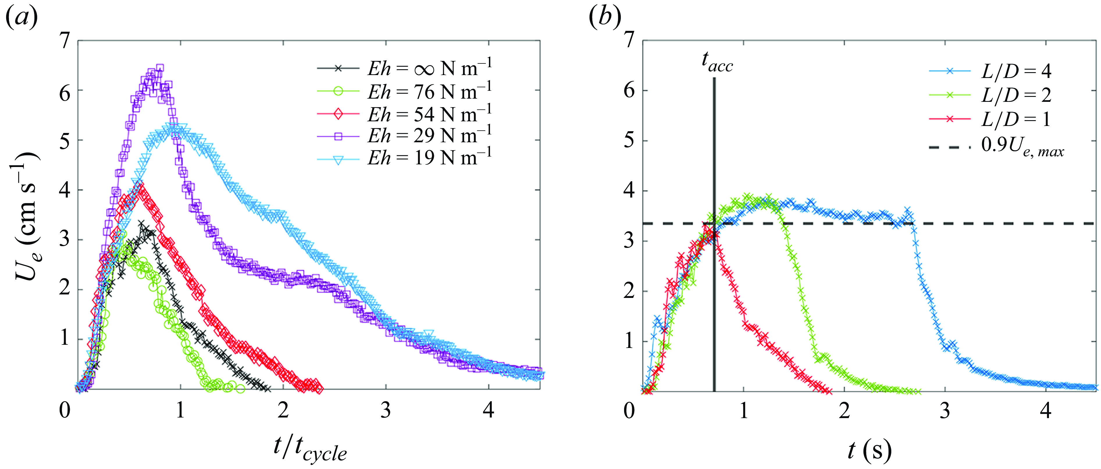
Figure 8. Temporal variation in vertical velocity spatially averaged across the nozzle exit ( $U_e$
) measured
$U_e$
) measured $0.19D$
below each nozzle: (a)
$0.19D$
below each nozzle: (a) $U_e$
for
$U_e$
for ${L}/{D}=1$
across all
${L}/{D}=1$
across all $Eh$
values for (
$Eh$
values for ( $t/t_{cycle} = 0-4.5$
); (b)
$t/t_{cycle} = 0-4.5$
); (b) $U_e$
for
$U_e$
for $Eh\approx \infty\,\rm N\,m^-{^1}$
(rigid), for all
$Eh\approx \infty\,\rm N\,m^-{^1}$
(rigid), for all ${L}/{D}$
values. Here,
${L}/{D}$
values. Here, $t_{acc}$
is defined as the time needed for the rigid nozzle to accelerate to 90 % of its maximum velocity.
$t_{acc}$
is defined as the time needed for the rigid nozzle to accelerate to 90 % of its maximum velocity.
The vertical velocity spatially averaged across the nozzle exit ( $U_e$
), measured
$U_e$
), measured $0.19D$
below the nozzles, is plotted for
$0.19D$
below the nozzles, is plotted for ${L}/{D}=1$
, in figure 8(a). As expected by the distance travelled by the PV in the vorticity plots in figures 5(a)–5(e),
${L}/{D}=1$
, in figure 8(a). As expected by the distance travelled by the PV in the vorticity plots in figures 5(a)–5(e), $U_e$
increases as
$U_e$
increases as $Eh$
is reduced to a maximum at
$Eh$
is reduced to a maximum at $Eh = 29\,\rm N\,m^-{^1}$
, and declines for
$Eh = 29\,\rm N\,m^-{^1}$
, and declines for $Eh = 19$
N/m. Furthermore, the time to reach the maximum
$Eh = 19$
N/m. Furthermore, the time to reach the maximum $U_e$
becomes delayed with decreased
$U_e$
becomes delayed with decreased $Eh$
. The
$Eh$
. The $Eh = 19\,\rm N\,m^-{^1}$
nozzle does not accelerate to its peak velocity until
$Eh = 19\,\rm N\,m^-{^1}$
nozzle does not accelerate to its peak velocity until $t/t_{cycle}=1.0$
, whereas the
$t/t_{cycle}=1.0$
, whereas the $Eh = 76\,\rm N\,m^-{^1}$
nozzle reaches its peak much quicker at
$Eh = 76\,\rm N\,m^-{^1}$
nozzle reaches its peak much quicker at $t/t_{cycle}=0.36$
.
$t/t_{cycle}=0.36$
.
To further examine the input flow conditions perturbed by the flexible nozzles, the output velocity from the rigid nozzle ( $Eh = \infty\,\rm N\,m^-{^1}$
) is plotted for all
$Eh = \infty\,\rm N\,m^-{^1}$
) is plotted for all ${L}/{D}$
values in figure 8(b). To compare the time scales of nozzle deformation with the input fluid flow, we define the time for the rigid nozzle to accelerate to 90 % of
${L}/{D}$
values in figure 8(b). To compare the time scales of nozzle deformation with the input fluid flow, we define the time for the rigid nozzle to accelerate to 90 % of $U_{e}$
as
$U_{e}$
as $t_{acc}\approx 0.71$
sec, as shown in figure 8(b). Next, we examine how the nozzle deformations vary with
$t_{acc}\approx 0.71$
sec, as shown in figure 8(b). Next, we examine how the nozzle deformations vary with $Eh$
to understand the kinematics affecting the flow fields.
$Eh$
to understand the kinematics affecting the flow fields.
Generally, each of the less stiff (more flexible) nozzles, ( $Eh = 54, 29, 19\,\rm N\,m^-{^1}$
), exhibited similar nozzle deformation kinematics. The deformation is characterised by 3 important time phases: (i) initial tip deflection, (ii) periodic oscillations, (iii) nozzle collapse and return to original state. These three stages are plotted with overlaid time-coloured plot images of the
$Eh = 54, 29, 19\,\rm N\,m^-{^1}$
), exhibited similar nozzle deformation kinematics. The deformation is characterised by 3 important time phases: (i) initial tip deflection, (ii) periodic oscillations, (iii) nozzle collapse and return to original state. These three stages are plotted with overlaid time-coloured plot images of the $Eh = 54\,\rm N\,m^-{^1}$
nozzle for
$Eh = 54\,\rm N\,m^-{^1}$
nozzle for ${L}/{D}=4$
in figures 9(a)–9(e). See Supplementary Material 2 for similar plots for each of the flexible nozzles. During phase (i), the initiation of deformation, a travelling wave, or series of travelling waves, propagates down the nozzle. In turn, the first oscillation inward generates the largest deflection at the nozzle tip while the pump is running, defined as
${L}/{D}=4$
in figures 9(a)–9(e). See Supplementary Material 2 for similar plots for each of the flexible nozzles. During phase (i), the initiation of deformation, a travelling wave, or series of travelling waves, propagates down the nozzle. In turn, the first oscillation inward generates the largest deflection at the nozzle tip while the pump is running, defined as $t_{max\;def}$
. This motion is shown for the
$t_{max\;def}$
. This motion is shown for the $Eh = 54\,\rm N\,m^-{^1}$
nozzle in figures 9(a) and 9(d). In phase (ii),
$Eh = 54\,\rm N\,m^-{^1}$
nozzle in figures 9(a) and 9(d). In phase (ii), $t_{max\;def}\lt t\lt t_{cycle}$
, the nozzles return to their initial position but with an over correction, expanding into the opposite plane of the initial tip deflection. These oscillations continue at varying frequencies depending on
$t_{max\;def}\lt t\lt t_{cycle}$
, the nozzles return to their initial position but with an over correction, expanding into the opposite plane of the initial tip deflection. These oscillations continue at varying frequencies depending on $Eh$
as shown in figures 9(b) and 9(e), until the pump turns off at
$Eh$
as shown in figures 9(b) and 9(e), until the pump turns off at $t/t_{cycle}=1$
marking the end of phase (ii). In phase (iii),
$t/t_{cycle}=1$
marking the end of phase (ii). In phase (iii), $t\gt t_{cycle}$
, each less stiff nozzle (
$t\gt t_{cycle}$
, each less stiff nozzle ( $Eh = 54, 29, 19\,\rm N\,m^-{^1}$
) collapses asymmetrically inward due to the decreased pressure from the quick decrease in velocity as the pump shuts off as shown from
$Eh = 54, 29, 19\,\rm N\,m^-{^1}$
) collapses asymmetrically inward due to the decreased pressure from the quick decrease in velocity as the pump shuts off as shown from $t_{cycle}\lt t\lt 2t_{cycle}$
in figures 9(c) and 9(f). The
$t_{cycle}\lt t\lt 2t_{cycle}$
in figures 9(c) and 9(f). The $Eh = 54\,\rm N\,m^-{^1}$
nozzle tip immediately reopens after partially collapsing. In contrast, the
$Eh = 54\,\rm N\,m^-{^1}$
nozzle tip immediately reopens after partially collapsing. In contrast, the $Eh = 29$
and
$Eh = 29$
and $19\,\rm N\,m^-{^1}$
nozzles fully collapse and remain in the collapsed position for 9 and 25 s, respectively, before reopening and oscillating back to their original position. Each nozzle consistently collapsed on one preferential axis for every trial.
$19\,\rm N\,m^-{^1}$
nozzles fully collapse and remain in the collapsed position for 9 and 25 s, respectively, before reopening and oscillating back to their original position. Each nozzle consistently collapsed on one preferential axis for every trial.
The $Eh = 76\,\rm N\,m^-{^1}$
nozzle was observed to have different kinematics than the less stiff nozzles. While the pump was moving, small-scale (
$Eh = 76\,\rm N\,m^-{^1}$
nozzle was observed to have different kinematics than the less stiff nozzles. While the pump was moving, small-scale ( $\approx {0.02D}$
) axisymmetric oscillations moved the nozzle slightly inward and outward until the pump stopped. Similar to the other nozzles, the pressure change at the nozzle exit created a small peak in deflection (
$\approx {0.02D}$
) axisymmetric oscillations moved the nozzle slightly inward and outward until the pump stopped. Similar to the other nozzles, the pressure change at the nozzle exit created a small peak in deflection ( $\approx {0.04D}$
) but the
$\approx {0.04D}$
) but the $Eh = 76\,\rm N\,m^-{^1}$
nozzle did not exhibit any collapse. Afterward, it oscillated back and forth until the viscous forces from the surrounding water damped the nozzle motion to a halt.
$Eh = 76\,\rm N\,m^-{^1}$
nozzle did not exhibit any collapse. Afterward, it oscillated back and forth until the viscous forces from the surrounding water damped the nozzle motion to a halt.
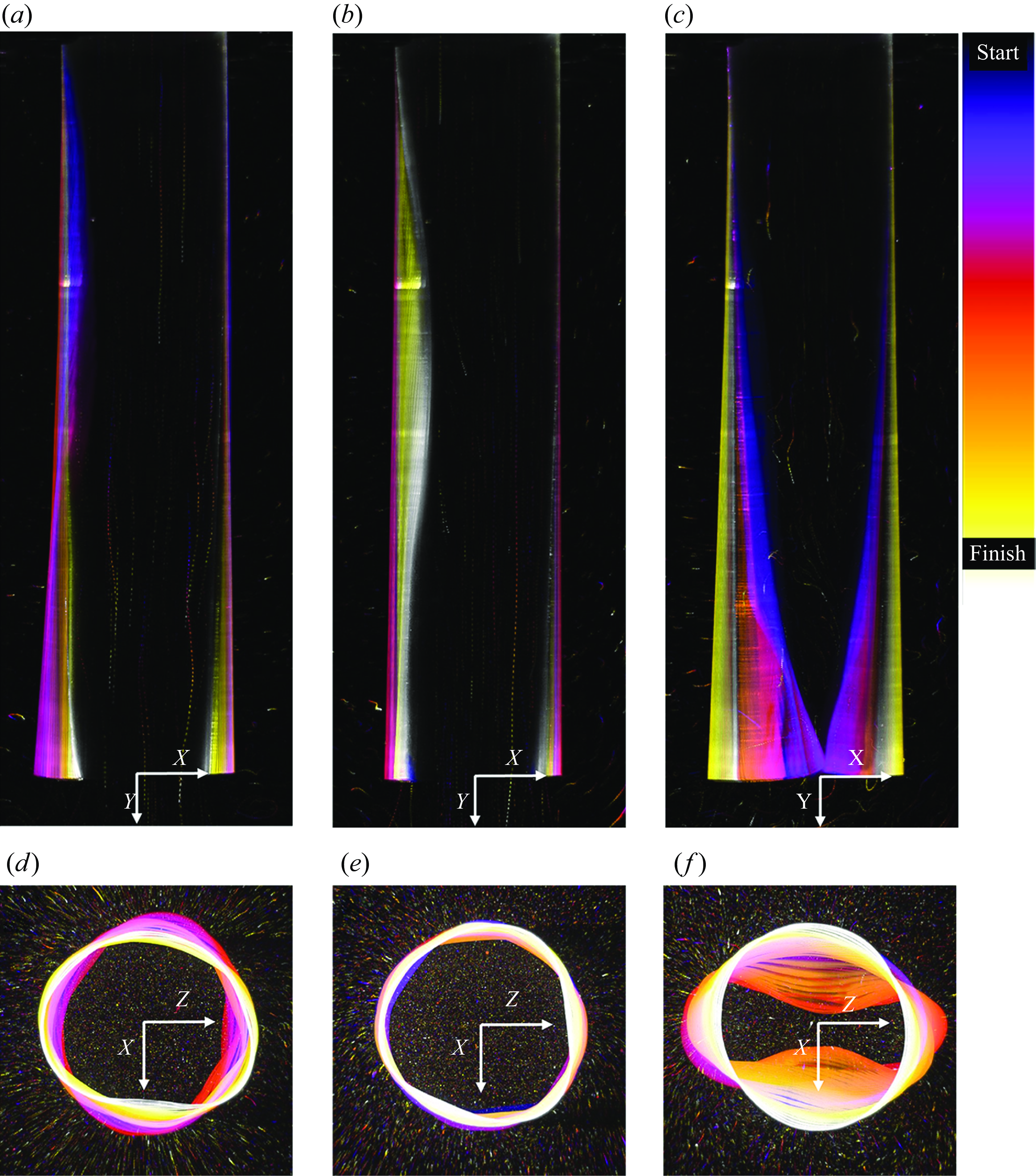
Figure 9. Imaging of the $Eh = 54\,\rm N\,m^-{^1}$
nozzle for
$Eh = 54\,\rm N\,m^-{^1}$
nozzle for ${L}/{D} = 4$
. The colour plot scale bar applies to each image, with the start and finish defined as follows in the panel descriptions. (a, d) Nozzle deformation for
${L}/{D} = 4$
. The colour plot scale bar applies to each image, with the start and finish defined as follows in the panel descriptions. (a, d) Nozzle deformation for $t = $ $0 - t_{max\;def}$
. (b, e) Nozzle deformation for
$0 - t_{max\;def}$
. (b, e) Nozzle deformation for $t = t_{max\;def} - t_{cycle}$
. (c, f) Nozzle deformation for
$t = t_{max\;def} - t_{cycle}$
. (c, f) Nozzle deformation for $t = t_{cycle} - 2t_{cycle}$
.
$t = t_{cycle} - 2t_{cycle}$
.
The bottom millimetre of the flexible nozzles was also quantitatively tracked. As expected, reducing the nozzle stiffness resulted in greater maximum deformation magnitudes at $t=t_{max\;def}$
, ranging from
$t=t_{max\;def}$
, ranging from $0.02D$
to
$0.02D$
to $0.19D$
for the
$0.19D$
for the $Eh = 76$
and
$Eh = 76$
and $29\,\rm N\,m^-{^1}$
nozzles, respectively. Although the
$29\,\rm N\,m^-{^1}$
nozzles, respectively. Although the $Eh=19\,\rm N\,m^-{^1}$
nozzle is the least stiff, the peak deformation was lower at only
$Eh=19\,\rm N\,m^-{^1}$
nozzle is the least stiff, the peak deformation was lower at only $0.15D$
. This will be discussed further in § 3.2. The
$0.15D$
. This will be discussed further in § 3.2. The $Eh = 54\,\rm N\,m^-{^1}$
tip deformation is shown in figure 10(a), illustrating the previously described deformation of the nozzle’s bottom millimetre. It is noted that prior to its inward deflection, the nozzle undergoes a small radial expansion due to jet acceleration and the positive internal pressure gradient. However, the magnitude of this deformation is significantly smaller than the large inward deflection and therefore does not appear prominently in figure 10(a). For reference, a plot illustrating the tip deformation of all the flexible nozzles is shown in figure 11(a). In figure 10(a), phases (i), (ii) and (iii) are delineated by orange, blue and green shading. In phase (i), orange, the nozzle tip shape becomes a slightly non-axisymmetric elongated oval at
$Eh = 54\,\rm N\,m^-{^1}$
tip deformation is shown in figure 10(a), illustrating the previously described deformation of the nozzle’s bottom millimetre. It is noted that prior to its inward deflection, the nozzle undergoes a small radial expansion due to jet acceleration and the positive internal pressure gradient. However, the magnitude of this deformation is significantly smaller than the large inward deflection and therefore does not appear prominently in figure 10(a). For reference, a plot illustrating the tip deformation of all the flexible nozzles is shown in figure 11(a). In figure 10(a), phases (i), (ii) and (iii) are delineated by orange, blue and green shading. In phase (i), orange, the nozzle tip shape becomes a slightly non-axisymmetric elongated oval at $t=t_{maxdef}$
. In phase (ii), green, the nozzle quickly returns to an approximately axisymmetric shape with smaller periodic oscillations. In phase (iii), blue, the nozzle collapses from the negative pressure gradient within the nozzle becoming highly non-axisymmetric. The nozzle tracking shown is from the XY plane to clearly show the large collapse. Once the nozzle reopens at
$t=t_{maxdef}$
. In phase (ii), green, the nozzle quickly returns to an approximately axisymmetric shape with smaller periodic oscillations. In phase (iii), blue, the nozzle collapses from the negative pressure gradient within the nozzle becoming highly non-axisymmetric. The nozzle tracking shown is from the XY plane to clearly show the large collapse. Once the nozzle reopens at $t=t_{free response}$
, the oscillation behaviour can be modelled as an underdamped free oscillation since no external forces are acting on the nozzle, other than the initial condition of starting in a collapsed state. This is highlighted with yellow shading, in figures 10(a) and 10(b). The natural frequency of the flexible nozzles is found by transforming the positional periodic motion of the free oscillations into the frequency domain using FFTs. The data used for this frequency analysis begin when the nozzle returns to its original position (
$t=t_{free response}$
, the oscillation behaviour can be modelled as an underdamped free oscillation since no external forces are acting on the nozzle, other than the initial condition of starting in a collapsed state. This is highlighted with yellow shading, in figures 10(a) and 10(b). The natural frequency of the flexible nozzles is found by transforming the positional periodic motion of the free oscillations into the frequency domain using FFTs. The data used for this frequency analysis begin when the nozzle returns to its original position ( $X/D=0$
) after collapsing due to the change in pressure. The data used for the FFT analysis were obtained from views from both the XY and XZ planes.
$X/D=0$
) after collapsing due to the change in pressure. The data used for the FFT analysis were obtained from views from both the XY and XZ planes.
For each nozzle, the frequency spectrum reveals a clear peak, indicating resonance at these specific frequencies under free oscillation, with an example frequency spectrum shown in figure 10(c). This resonant peak corresponds to the damped natural frequency ( $\omega _{d}$
) for each nozzle. A summary of the variation of
$\omega _{d}$
) for each nozzle. A summary of the variation of $\omega _d$
with
$\omega _d$
with $Eh$
is shown in figure 10(d), which is intuitive in that the stiffer nozzles have a higher
$Eh$
is shown in figure 10(d), which is intuitive in that the stiffer nozzles have a higher $\omega _d$
values as stiffness scales with natural frequency. These
$\omega _d$
values as stiffness scales with natural frequency. These $\omega _{d}$
values can be incredibly useful in that they can be used to predict the timing of
$\omega _{d}$
values can be incredibly useful in that they can be used to predict the timing of $t_{max\;def}$
. The maximum variation in measured
$t_{max\;def}$
. The maximum variation in measured $\omega _{d}$
, was for the
$\omega _{d}$
, was for the $Eh = 54\,\rm N\,m^-{^1}$
nozzle where
$Eh = 54\,\rm N\,m^-{^1}$
nozzle where $\omega _{d} = 0.737 \pm 0.013$
Hz based on the 95 % confidence interval.
$\omega _{d} = 0.737 \pm 0.013$
Hz based on the 95 % confidence interval.
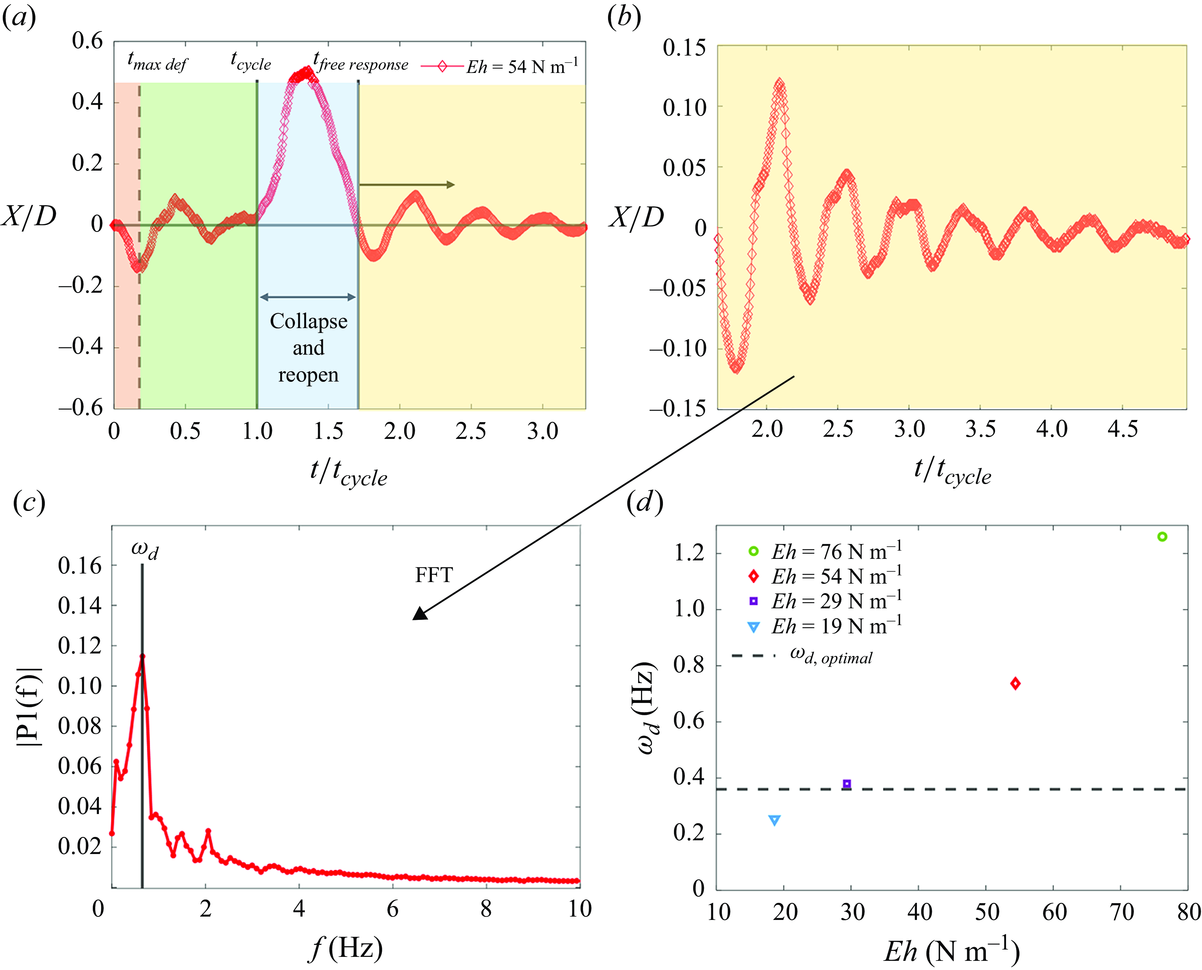
Figure 10. (a) Temporal variation of position ( $X/D$
) for the
$X/D$
) for the $Eh=54\,\rm N\,m^-{^1}$
nozzle tip. The
$Eh=54\,\rm N\,m^-{^1}$
nozzle tip. The $t_{free reponse}$
line indicates the start of the data used to find the frequency spectrum. (b) Tracked nozzle deflections used for FFT to quantify the frequency spectrum. The start is initiated by when the nozzle tip passes its original position (
$t_{free reponse}$
line indicates the start of the data used to find the frequency spectrum. (b) Tracked nozzle deflections used for FFT to quantify the frequency spectrum. The start is initiated by when the nozzle tip passes its original position ( $X/D=0$
), after undergoing collapse due to the negative pressure gradient. (c) Frequency spectrum obtained from the positional data. Here,
$X/D=0$
), after undergoing collapse due to the negative pressure gradient. (c) Frequency spectrum obtained from the positional data. Here, $\omega _{d}$
is identified as the most prevalent frequency in the frequency domain. (d) Value of
$\omega _{d}$
is identified as the most prevalent frequency in the frequency domain. (d) Value of $\omega _{d}$
for the different
$\omega _{d}$
for the different $Eh$
nozzles found using the same process as outlined here.
$Eh$
nozzles found using the same process as outlined here.
Choi & Park (Reference Choi and Park2022, Reference Choi and Park2024) proposed that synchronising the maximum deformation with the input fluid acceleration, i.e. timing the release of elastic energy to the fluid, creates the optimal conditions for thrust from a starting jet. Based on this, we hypothesise that the optimal nozzle stiffness for increasing thrust can be predicted using the damped natural frequency of the nozzle, such that the optimal condition will occur when $t_{acc}=t_{max\;def}$
, where
$t_{acc}=t_{max\;def}$
, where $t_{acc}$
is the time to reach peak fluid acceleration from the rigid nozzle, and
$t_{acc}$
is the time to reach peak fluid acceleration from the rigid nozzle, and $t_{max\;def}$
is the time of maximum nozzle deformation while the pump is running. Using the damped natural frequency,
$t_{max\;def}$
is the time of maximum nozzle deformation while the pump is running. Using the damped natural frequency, $\omega _d$
, of each nozzle we predict
$\omega _d$
, of each nozzle we predict $t_{max\;def}$
to occur at
$t_{max\;def}$
to occur at ${1}/{4}$
of an oscillatory cycle, i.e.
${1}/{4}$
of an oscillatory cycle, i.e. $t_{max\;def} = {1}/{4\omega _{d}}$
. If
$t_{max\;def} = {1}/{4\omega _{d}}$
. If $t_{acc}=t_{max\;def}= {1}/{4\omega _{d}}$
, we can estimate the optimal nozzle damped frequency,
$t_{acc}=t_{max\;def}= {1}/{4\omega _{d}}$
, we can estimate the optimal nozzle damped frequency, $\omega _{d, optimal}$
, for the present flow conditions (measured
$\omega _{d, optimal}$
, for the present flow conditions (measured $t_{acc}$
). Under the current flow conditions,
$t_{acc}$
). Under the current flow conditions, $\omega _{d, optimal}=0.36\,\rm Hz$
. For the tested nozzles, the
$\omega _{d, optimal}=0.36\,\rm Hz$
. For the tested nozzles, the $Eh = 29\,\rm N\,m^-{^1}$
nozzle with
$Eh = 29\,\rm N\,m^-{^1}$
nozzle with $\omega _{d} = 0.38 \pm 0.008\,\rm Hz$
Hz is closest to
$\omega _{d} = 0.38 \pm 0.008\,\rm Hz$
Hz is closest to $\omega _{d, optimal}$
, shown in figure 10(d). In the following section, we will confirm this prediction of the optimal nozzle stiffness (nozzle stiffness that will lead to greatest increase in thrust) by further examining the fluid output for each nozzle stiffness and
$\omega _{d, optimal}$
, shown in figure 10(d). In the following section, we will confirm this prediction of the optimal nozzle stiffness (nozzle stiffness that will lead to greatest increase in thrust) by further examining the fluid output for each nozzle stiffness and $L/D$
.
$L/D$
.
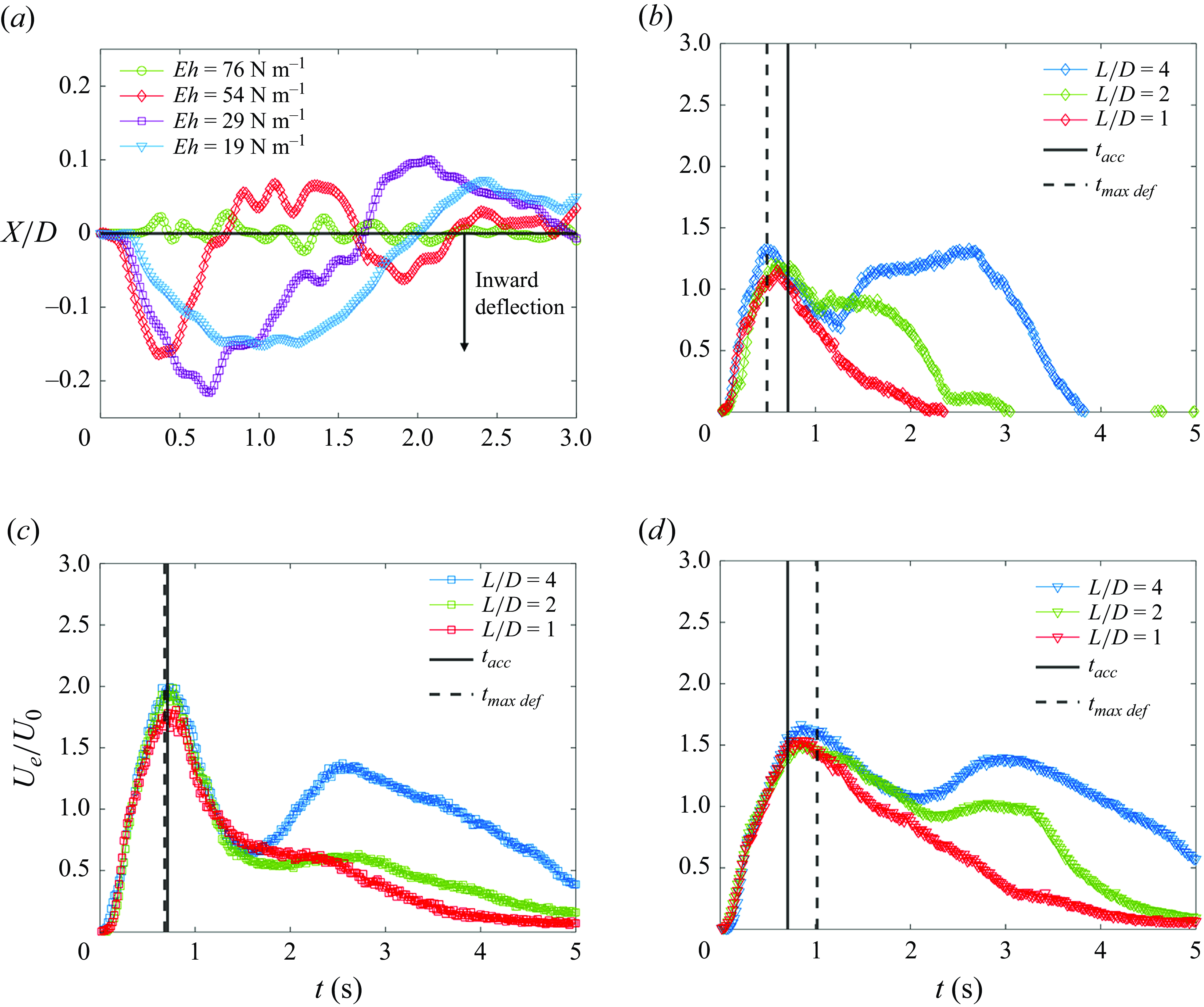
Figure 11. (a) Temporal variation in nozzle tip deflection for ${L}/{D}=4$
. (b-c) Spatially averaged velocity measured
${L}/{D}=4$
. (b-c) Spatially averaged velocity measured $0.19D$
beneath the nozzle exit (
$0.19D$
beneath the nozzle exit ( $U_e$
) for
$U_e$
) for $Eh = 54, 29, 19\,\rm N\,m^-{^1}$
for all
$Eh = 54, 29, 19\,\rm N\,m^-{^1}$
for all ${L}/{D}$
normalied by the steadystate rigid nozzle velocity (
${L}/{D}$
normalied by the steadystate rigid nozzle velocity ( $U_0$
) measured for each respective
$U_0$
) measured for each respective ${L}/{D}$
; (b)
${L}/{D}$
; (b) $U_e/U_0$
for
$U_e/U_0$
for $Eh = 54\,\rm N\,m^-{^1}$
; (c)
$Eh = 54\,\rm N\,m^-{^1}$
; (c) $U_e/U_0$
for
$U_e/U_0$
for $Eh = 29\,\rm N\,m^-{^1}$
; (d)
$Eh = 29\,\rm N\,m^-{^1}$
; (d) $U_e/U_0$
for
$U_e/U_0$
for $Eh = 19\,\rm N\,m^-{^1}$
.
$Eh = 19\,\rm N\,m^-{^1}$
.
3.2. Optimal conditions, fluid impulse and circulation
To further investigate the relationship between $t_{max\;def}$
and
$t_{max\;def}$
and $t_{acc}$
, we examine the measured output velocities from the
$t_{acc}$
, we examine the measured output velocities from the $Eh = 54, 29$
and
$Eh = 54, 29$
and $19\,\rm N\,m^-{^1}$
nozzles, all of which have different
$19\,\rm N\,m^-{^1}$
nozzles, all of which have different $t_{max\;def}$
based on their respective
$t_{max\;def}$
based on their respective $\omega _d$
. Three different timing scenarios can occur (
$\omega _d$
. Three different timing scenarios can occur ( $t_{acc}\gt t_{max\;def}$
,
$t_{acc}\gt t_{max\;def}$
, $t_{acc}\lt t_{max\;def}$
,
$t_{acc}\lt t_{max\;def}$
, $t_{acc}=t_{max\;def}$
), which is summarised by the nozzle tip deflection plot in figure 11(a) and the output velocity profiles from the
$t_{acc}=t_{max\;def}$
), which is summarised by the nozzle tip deflection plot in figure 11(a) and the output velocity profiles from the $Eh = 54, 29$
and
$Eh = 54, 29$
and $19\,\rm N\,m^-{^1}$
nozzles in figures 11(b)–11(d). The
$19\,\rm N\,m^-{^1}$
nozzles in figures 11(b)–11(d). The $Eh = 76\,\rm N\,m^-{^1}$
nozzle velocity is not plotted as it matches the same timing scenario as the
$Eh = 76\,\rm N\,m^-{^1}$
nozzle velocity is not plotted as it matches the same timing scenario as the $Eh = 54$
N/m nozzle, but with much lower magnitude. For reference,
$Eh = 54$
N/m nozzle, but with much lower magnitude. For reference, $t_{max\;def}$
can be interpreted from figure 11(a) as the time to reach the first big peak in inward deflection.
$t_{max\;def}$
can be interpreted from figure 11(a) as the time to reach the first big peak in inward deflection.
In the first scenario, where $t_{acc}\gt t_{max\;def}$
, the nozzle tip reaches maximum inward deformation prior to the end of input fluid acceleration of the unperturbed flow. This condition is met by the
$t_{acc}\gt t_{max\;def}$
, the nozzle tip reaches maximum inward deformation prior to the end of input fluid acceleration of the unperturbed flow. This condition is met by the $Eh = 54$
N m–1 nozzle, where there is a slight enhancement in peak output velocity shown in figure 11(b). Here the nozzle contraction occurs at
$Eh = 54$
N m–1 nozzle, where there is a slight enhancement in peak output velocity shown in figure 11(b). Here the nozzle contraction occurs at $t_{max\;def} = 0.65t_{acc}$
, after which the velocity decreases, as elastic energy is no longer being supplied to the flow after
$t_{max\;def} = 0.65t_{acc}$
, after which the velocity decreases, as elastic energy is no longer being supplied to the flow after $t_{max\;def}$
. In contrast, after
$t_{max\;def}$
. In contrast, after $t_{max\;def}$
the nozzle extracts energy back from the fluid to re-expand to its original position. In the re-expansion process a suction velocity is generated that counters the input flow direction and causes a decline in output velocity as the input fluid flow continues to accelerate until
$t_{max\;def}$
the nozzle extracts energy back from the fluid to re-expand to its original position. In the re-expansion process a suction velocity is generated that counters the input flow direction and causes a decline in output velocity as the input fluid flow continues to accelerate until $t_{acc}$
. This mismatch in timing results in the output velocity profile reaching the maximum velocity at time
$t_{acc}$
. This mismatch in timing results in the output velocity profile reaching the maximum velocity at time $t_{max vel}$
, where
$t_{max vel}$
, where $t_{max\;def}\lt t_{max vel} \lt t_{acc}$
, as the nozzle re-expansion temporarily impedes the output velocity growth after
$t_{max\;def}\lt t_{max vel} \lt t_{acc}$
, as the nozzle re-expansion temporarily impedes the output velocity growth after $t_{max\;def}$
.
$t_{max\;def}$
.
The second scenario ( $t_{acc}\lt t_{max\;def}$
) is met by the
$t_{acc}\lt t_{max\;def}$
) is met by the $Eh=19\,\rm N\,m^-{^1}$
nozzle where the nozzle contraction occurs at
$Eh=19\,\rm N\,m^-{^1}$
nozzle where the nozzle contraction occurs at $t_{max\;def} = 1.4t_{acc}$
shown in figure 11(d). In this case, elastic energy supplied by the nozzle is transferred to the fluid throughout all of
$t_{max\;def} = 1.4t_{acc}$
shown in figure 11(d). In this case, elastic energy supplied by the nozzle is transferred to the fluid throughout all of $t_{acc}$
, which supplements the velocity growth for a much longer period resulting in higher peak velocities compared with
$t_{acc}$
, which supplements the velocity growth for a much longer period resulting in higher peak velocities compared with $Eh = 54\,\rm N\,m^-{^1}$
. However, the response of the nozzle lags behind the input acceleration of the fluid, so a portion of the elastic energy stored within the nozzle has not been fully transferred to the flow before
$Eh = 54\,\rm N\,m^-{^1}$
. However, the response of the nozzle lags behind the input acceleration of the fluid, so a portion of the elastic energy stored within the nozzle has not been fully transferred to the flow before $t_{acc}$
. As the input acceleration ends at
$t_{acc}$
. As the input acceleration ends at $t_{acc}$
, there is a decrease in the growth rate of velocity. However, as the nozzle is still supplying elastic energy to the fluid, the velocity continues to grow until time
$t_{acc}$
, there is a decrease in the growth rate of velocity. However, as the nozzle is still supplying elastic energy to the fluid, the velocity continues to grow until time $t_{max vel}$
where
$t_{max vel}$
where $t_{acc}\lt t_{max vel} \lt t_{max\;def}$
. Due to the delay in
$t_{acc}\lt t_{max vel} \lt t_{max\;def}$
. Due to the delay in $t_{max\;def}$
, the acceleration is slower, and the peak velocity is lower compared with the optimal case.
$t_{max\;def}$
, the acceleration is slower, and the peak velocity is lower compared with the optimal case.
For the optimal conditions, the $Eh=29\,\rm N\,m^-{^1}$
nozzle tip reaches peak inward deflection at the same exact time as the end of the input fluid acceleration,
$Eh=29\,\rm N\,m^-{^1}$
nozzle tip reaches peak inward deflection at the same exact time as the end of the input fluid acceleration, $t_{max\;def} = t_{acc}$
. This results in all of the elastic energy stored in the nozzle being imparted to the flow within
$t_{max\;def} = t_{acc}$
. This results in all of the elastic energy stored in the nozzle being imparted to the flow within $t_{acc}$
as shown in figure 11(c), as well as a greater tip deflection shown in figure 11(a). In this case, all of the elastic energy from the nozzle is supplied to the fluid within the same duration in which the input flow is accelerating, maximising the growth in the fluid velocity. Additionally, it is understood that the pressure change from acceleration to steady velocity input flow and the formation of a vortex ring creates a low pressure region at the nozzle tip at the same time as
$t_{acc}$
as shown in figure 11(c), as well as a greater tip deflection shown in figure 11(a). In this case, all of the elastic energy from the nozzle is supplied to the fluid within the same duration in which the input flow is accelerating, maximising the growth in the fluid velocity. Additionally, it is understood that the pressure change from acceleration to steady velocity input flow and the formation of a vortex ring creates a low pressure region at the nozzle tip at the same time as $t_{max\;def}$
, creating a positive feedback loop that magnifies the inward tip deflection and output (Gao et al. Reference Gao, Wang, Yu and Chyu2020). This behaviour is seen as a slight inflection point for all of the flexible nozzles in figure 11(a) at
$t_{max\;def}$
, creating a positive feedback loop that magnifies the inward tip deflection and output (Gao et al. Reference Gao, Wang, Yu and Chyu2020). This behaviour is seen as a slight inflection point for all of the flexible nozzles in figure 11(a) at $t\approx t_{acc}$
, which results in the
$t\approx t_{acc}$
, which results in the $Eh = 29\,\rm N\,m^-{^1}$
nozzle deflecting an additional
$Eh = 29\,\rm N\,m^-{^1}$
nozzle deflecting an additional $0.027{X}/{D}$
. Importantly, the nozzle deformation behaviour is consistent across all
$0.027{X}/{D}$
. Importantly, the nozzle deformation behaviour is consistent across all ${L}/{D}$
values during the fluid acceleration period, ensuring that this optimal timing is effective regardless of ejected volume.
${L}/{D}$
values during the fluid acceleration period, ensuring that this optimal timing is effective regardless of ejected volume.
For the $Eh = 54, 29$
and
$Eh = 54, 29$
and $19\,\rm N\,m^-{^1}$
nozzles with
$19\,\rm N\,m^-{^1}$
nozzles with ${L}/{D} = 2$
and
${L}/{D} = 2$
and $4$
, there is a decline in output velocity after
$4$
, there is a decline in output velocity after $t_{max\;def}$
, or
$t_{max\;def}$
, or $t_{acc}$
, depending on which occurs later, despite the input fluid velocity remaining constant. This decrease is attributed to the nozzle re-expanding back to its original position after
$t_{acc}$
, depending on which occurs later, despite the input fluid velocity remaining constant. This decrease is attributed to the nozzle re-expanding back to its original position after $t_{max\;def}$
, creating a counter flow opposing the input flow conditions and extracting energy back from the fluid to reopen. As the nozzles return to their original position, the piston motion continues and then accelerates the fluid back to the input velocity until
$t_{max\;def}$
, creating a counter flow opposing the input flow conditions and extracting energy back from the fluid to reopen. As the nozzles return to their original position, the piston motion continues and then accelerates the fluid back to the input velocity until $t_{cycle}$
. In contrast, for
$t_{cycle}$
. In contrast, for ${L}/{D}=1$
,
${L}/{D}=1$
, $t_{cycle}$
occurs before the nozzle can completely return to its original position, negating the need to overcome the entire counter flow generated by the nozzle reopening, maximising the relative flow output. The effect of
$t_{cycle}$
occurs before the nozzle can completely return to its original position, negating the need to overcome the entire counter flow generated by the nozzle reopening, maximising the relative flow output. The effect of ${L}/{D}$
is explored further in § 3.3.
${L}/{D}$
is explored further in § 3.3.
To compare the vorticity generated as $Eh$
is varied, the total circulation (
$Eh$
is varied, the total circulation ( $\Gamma$
) is calculated using
$\Gamma$
) is calculated using
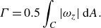 \begin{equation} \Gamma = 0.5 \int _{C} |\omega _z| \, {\rm d}A .\end{equation}
The 90 % vorticity contour is chosen as the integration area, $C$
, within the field of view defined by
$C$
, within the field of view defined by $-1.5\lt x/D\lt 1.5$
, and
$-1.5\lt x/D\lt 1.5$
, and $-0.5\lt y/D\lt 5.5$
. Here,
$-0.5\lt y/D\lt 5.5$
. Here, $|\omega _{z}|$
is the vorticity perpendicular to the measurement plane, as the flow is axisymmetric (
$|\omega _{z}|$
is the vorticity perpendicular to the measurement plane, as the flow is axisymmetric ( $\omega _x = \omega _y = 0$
). Circulation is non-dimensionalised by dividing the temporal data by the circulation generated by the rigid nozzle (
$\omega _x = \omega _y = 0$
). Circulation is non-dimensionalised by dividing the temporal data by the circulation generated by the rigid nozzle ( $\Gamma _0$
) at
$\Gamma _0$
) at $t/t_{cycle}=1$
. Figure12(a) shows the temporal variation of total circulation (
$t/t_{cycle}=1$
. Figure12(a) shows the temporal variation of total circulation ( ${\Gamma }/{\Gamma _{0}}|_{t/t_{cycle}=1}$
) as
${\Gamma }/{\Gamma _{0}}|_{t/t_{cycle}=1}$
) as $Eh$
is varied for
$Eh$
is varied for ${L}/{D}=1$
. Similar to the trend observed to this point, the least stiff nozzles,
${L}/{D}=1$
. Similar to the trend observed to this point, the least stiff nozzles, $Eh=19\,\rm N\,m^-{^1}$
N/m and
$Eh=19\,\rm N\,m^-{^1}$
N/m and $Eh=29\,\rm N\,m^-{^1}$
, produced the largest relative circulation,
$Eh=29\,\rm N\,m^-{^1}$
, produced the largest relative circulation, ${\Gamma }/{\Gamma _{0}} = 2.87$
and
${\Gamma }/{\Gamma _{0}} = 2.87$
and $2.91$
, respectively. However, the
$2.91$
, respectively. However, the $Eh = 19\,\rm N\,m^-{^1}$
, nozzle requires nearly twice as much time (
$Eh = 19\,\rm N\,m^-{^1}$
, nozzle requires nearly twice as much time ( $t/t_{cycle}=2$
) to reach peak circulation compared with the
$t/t_{cycle}=2$
) to reach peak circulation compared with the $Eh = 29\,\rm N\,m^-{^1}$
nozzle (
$Eh = 29\,\rm N\,m^-{^1}$
nozzle ( $t/t_{cycle}=1.1$
). It is noted that
$t/t_{cycle}=1.1$
). It is noted that $\Gamma$
is found to be equal in both the parallel (XY) and perpendicular (XZ) planes to the preferential axis of nozzle collapse for all experiments. See Appendix A for circulation plots comparing the two measurement planes.
$\Gamma$
is found to be equal in both the parallel (XY) and perpendicular (XZ) planes to the preferential axis of nozzle collapse for all experiments. See Appendix A for circulation plots comparing the two measurement planes.
To quantify the effect of nozzle stiffness on the output thrust, hydrodynamic impulse is calculated using (Saffman Reference Saffman1993)
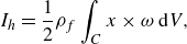 \begin{equation} I_h = \frac {1}{2}\rho _{f}\int _{C}x\times \omega \ {\rm d}V, \end{equation}

Figure 12. Temporal variation in total circulation and impulse for ${L}/{D}=1$
. (a) Total circulation (
${L}/{D}=1$
. (a) Total circulation ( $\Gamma$
) normalised by the rigid nozzle (
$\Gamma$
) normalised by the rigid nozzle ( $Eh=\infty$
) circulation at
$Eh=\infty$
) circulation at $t/t_{cycle}=1$
. (b) Total impulse (
$t/t_{cycle}=1$
. (b) Total impulse ( $I$
), normalised by the rigid nozzle (
$I$
), normalised by the rigid nozzle ( $Eh=\infty\,\rm N\,m^-{^1}$
) impulse at
$Eh=\infty\,\rm N\,m^-{^1}$
) impulse at $t/t_{cycle}=1$
. Legend is the same for (a) and (b).
$t/t_{cycle}=1$
. Legend is the same for (a) and (b).
where cylindrical coordinates are used with position vector $\boldsymbol{x} = (r, \theta, y)$
with the origin located at the centre of the nozzle exit, with positive
$\boldsymbol{x} = (r, \theta, y)$
with the origin located at the centre of the nozzle exit, with positive $y$
in flow direction. The vorticity vector is simplified and given as
$y$
in flow direction. The vorticity vector is simplified and given as $\omega _z$
for consistency. Considering
$\omega _z$
for consistency. Considering ${\rm d}V = 2\pi r{\rm d}A$
, hydrodynamic impulse can be calculated as
${\rm d}V = 2\pi r{\rm d}A$
, hydrodynamic impulse can be calculated as $I_h = \pi \rho _{f} \int _{C} r^2 |\omega _{z}|{\rm d}A$
. Here,
$I_h = \pi \rho _{f} \int _{C} r^2 |\omega _{z}|{\rm d}A$
. Here, $\rho _{f}$
is the fluid density at room temperature and
$\rho _{f}$
is the fluid density at room temperature and $r$
is the radial distance to each integration element from the nozzle centre line. In figure 12(b), the temporal distribution of impulse (
$r$
is the radial distance to each integration element from the nozzle centre line. In figure 12(b), the temporal distribution of impulse ( ${I_h}/{I_0}|_{t/t_{cycle}=1}$
) is plotted, where
${I_h}/{I_0}|_{t/t_{cycle}=1}$
) is plotted, where $I_0$
is the rigid nozzle impulse measured at
$I_0$
is the rigid nozzle impulse measured at $t/t_{cycle}=1$
. The measured hydrodynamic impulse increases as
$t/t_{cycle}=1$
. The measured hydrodynamic impulse increases as $Eh$
declines (becomes less stiff), up to
$Eh$
declines (becomes less stiff), up to $Eh=29\,\rm N\,m^-{^1}$
. Similar to circulation, the impulse generated by the least stiff nozzle (
$Eh=29\,\rm N\,m^-{^1}$
. Similar to circulation, the impulse generated by the least stiff nozzle ( $Eh=19\,\rm N\,m^-{^1}$
) eventually achieves similar amounts of hydrodynamic impulse to the
$Eh=19\,\rm N\,m^-{^1}$
) eventually achieves similar amounts of hydrodynamic impulse to the $Eh=29\,\rm N\,m^-{^1}$
nozzle, but not until
$Eh=29\,\rm N\,m^-{^1}$
nozzle, but not until $t/t_{cycle}=2.75$
, compared with
$t/t_{cycle}=2.75$
, compared with $t/t_{cycle}=0.8$
, which is predicted to result in much lower force production which scales with impulse generated per time (Saffman Reference Saffman1993). As previously discussed in § 3.1, the flexible nozzles collapse under the negative pressure gradient formed upon fluid deceleration. Importantly, the hydrodynamic impulse generated from the flexible nozzles has no dip at
$t/t_{cycle}=0.8$
, which is predicted to result in much lower force production which scales with impulse generated per time (Saffman Reference Saffman1993). As previously discussed in § 3.1, the flexible nozzles collapse under the negative pressure gradient formed upon fluid deceleration. Importantly, the hydrodynamic impulse generated from the flexible nozzles has no dip at $t=t_{cycle}$
, which would indicate a loss in the pressure impulse (Gao et al. Reference Gao, Wang, Yu and Chyu2020). In contrast, the unfavourable pressure gradient formed within the rigid nozzle results in a clear loss in hydrodynamic impulse at
$t=t_{cycle}$
, which would indicate a loss in the pressure impulse (Gao et al. Reference Gao, Wang, Yu and Chyu2020). In contrast, the unfavourable pressure gradient formed within the rigid nozzle results in a clear loss in hydrodynamic impulse at $t=t_{cycle}$
due to the generation of negative pressure impulse, as seen in figure 12(b). Through the nozzle collapse mechanism, the negative pressure gradient is instead suppressed as shown in figure 12(b), resulting in no additional losses in hydrodynamic impulse. A summary of the measured impulse at
$t=t_{cycle}$
due to the generation of negative pressure impulse, as seen in figure 12(b). Through the nozzle collapse mechanism, the negative pressure gradient is instead suppressed as shown in figure 12(b), resulting in no additional losses in hydrodynamic impulse. A summary of the measured impulse at $t_{cycle}$
across all
$t_{cycle}$
across all $Eh$
and
$Eh$
and ${L}/{D}$
is presented in figure 13(a). These results confirm that the
${L}/{D}$
is presented in figure 13(a). These results confirm that the $Eh = 29\,\rm N\,m^-{^1}$
nozzle produces the largest increase in thrust or hydrodynamic impulse as predicted from our nozzle deformation measurements (optimal nozzle condition), and any increase or decrease in
$Eh = 29\,\rm N\,m^-{^1}$
nozzle produces the largest increase in thrust or hydrodynamic impulse as predicted from our nozzle deformation measurements (optimal nozzle condition), and any increase or decrease in $\omega _{d}$
results in a reduction in output thrust.
$\omega _{d}$
results in a reduction in output thrust.
Interestingly, as a result of these differing measured output velocities with nozzle stiffness (despite the same kinematic input), the fluid slug length expelled also differs with flexibility. Specifically, the flexible nozzle deformations and collapse after $t/t_{cycle}=1$
expel additional fluid relative to the rigid case, increasing the total ejected volume that can positively contribute to the circulation of the vortex ring. However, after sufficient time the nozzle reopens, refilling itself returning the total ejected volume to equilibrium for mass conservation. The nozzle refilling process will be discussed further in § 3.4. As such, the effective expelled fluid slug length needs to be derived by integrating the
$t/t_{cycle}=1$
expel additional fluid relative to the rigid case, increasing the total ejected volume that can positively contribute to the circulation of the vortex ring. However, after sufficient time the nozzle reopens, refilling itself returning the total ejected volume to equilibrium for mass conservation. The nozzle refilling process will be discussed further in § 3.4. As such, the effective expelled fluid slug length needs to be derived by integrating the $U_e$
profiles and dividing by the nozzle diameter to yield
$U_e$
profiles and dividing by the nozzle diameter to yield $({L}/{D})_{eff} ={1}/{D} \int U_e(t){\rm d}t$
. The circulation produced by the different nozzles should scale linearly with increasing
$({L}/{D})_{eff} ={1}/{D} \int U_e(t){\rm d}t$
. The circulation produced by the different nozzles should scale linearly with increasing $({L}/{D})_{eff}$
(Didden Reference Didden1979). This is confirmed in figure13(b), where the data show a linear trend as expected from Gharib et al. (Reference Gharib, Rambod and Shariff1998).
$({L}/{D})_{eff}$
(Didden Reference Didden1979). This is confirmed in figure13(b), where the data show a linear trend as expected from Gharib et al. (Reference Gharib, Rambod and Shariff1998).
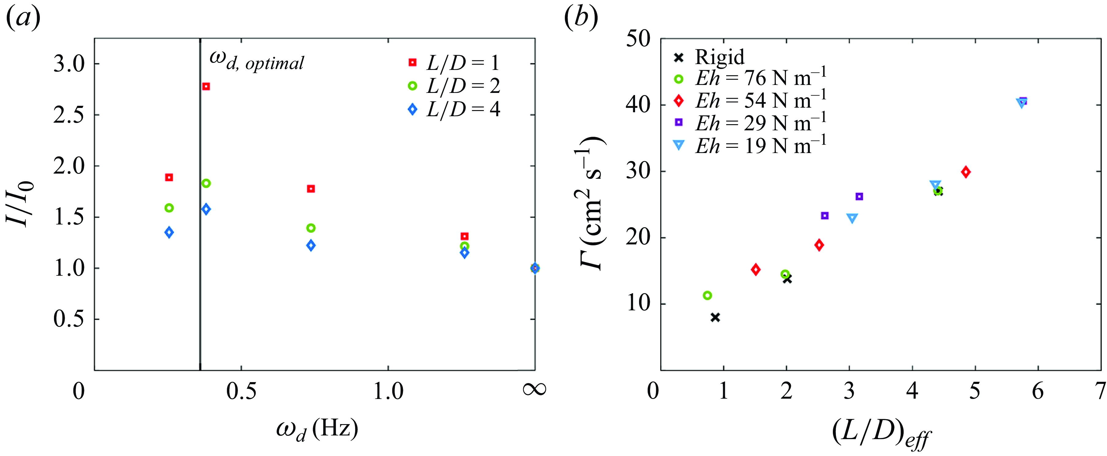
Figure 13. Summary of the total measured impulse and circulation from each nozzle over all ${L}/{D}$
values. (a) Normalised impulse plotted versus damped natural frequency
${L}/{D}$
values. (a) Normalised impulse plotted versus damped natural frequency $\omega _d$
, with the predicted optimal
$\omega _d$
, with the predicted optimal $\omega _{d, optimal}$
condition shown. (b) Measured total circulation versus effective ejected volume (
$\omega _{d, optimal}$
condition shown. (b) Measured total circulation versus effective ejected volume ( $({L}/{D})_{eff}$
).
$({L}/{D})_{eff}$
).
The lowest ejected volume, ${L}/{D}=1$
, resulted in the highest normalised impulse compared with the rigid nozzle data, as shown in figure 13(a). This is contributed to four aspects: initial increase of fluid velocity from the nozzle elastic energy, no loss in pressure impulse due to fluid deceleration, high relative increase in
${L}/{D}=1$
, resulted in the highest normalised impulse compared with the rigid nozzle data, as shown in figure 13(a). This is contributed to four aspects: initial increase of fluid velocity from the nozzle elastic energy, no loss in pressure impulse due to fluid deceleration, high relative increase in $({L}/{D})_{eff}$
and formation of a single coherent vortex structure. The first aspect is related to the flexible nozzles imparting elastic energy when
$({L}/{D})_{eff}$
and formation of a single coherent vortex structure. The first aspect is related to the flexible nozzles imparting elastic energy when $t\lt t_{max\;def}$
, which occurs early in the fluid expulsion process. As the deformation behaviour of the nozzles, and thus elastic energy supplied, is approximately constant across all
$t\lt t_{max\;def}$
, which occurs early in the fluid expulsion process. As the deformation behaviour of the nozzles, and thus elastic energy supplied, is approximately constant across all ${L}/{D}$
, the relative gain of this energy is maximised for the lowest ejected volume. Additionally, after
${L}/{D}$
, the relative gain of this energy is maximised for the lowest ejected volume. Additionally, after $t_{max\;def}$
the flexible nozzles extract energy back from the flow to re-expand, which creates a suction velocity that counters the input flow direction. For
$t_{max\;def}$
the flexible nozzles extract energy back from the flow to re-expand, which creates a suction velocity that counters the input flow direction. For ${L}/{D}=1$
, the pump turns off when the nozzle re-expansion process is taking place, whereas the larger ejected volumes must completely overcome this suction velocity to continue to expel additional fluid.
${L}/{D}=1$
, the pump turns off when the nozzle re-expansion process is taking place, whereas the larger ejected volumes must completely overcome this suction velocity to continue to expel additional fluid.
The second aspect, the suppression of the negative pressure gradient from nozzle collapse, is amplified at lower ejected volumes. For lower ejected volumes, a slight loss of hydrodynamic impulse due to negative pressure impulse has a proportionally larger effect on the total produced. The flexible nozzles collapse inward when this unfavourable pressure region is formed, and in turn not only suppresses the negative impacts of the negative pressure region, but also expel additional fluid volume.
The third aspect, the relative increase in effective ejected volume, $({L}/{D})_{eff}$
, is maximised at lower ejected volumes. The added volume from the nozzle deformation is approximately constant across all
$({L}/{D})_{eff}$
, is maximised at lower ejected volumes. The added volume from the nozzle deformation is approximately constant across all ${L}/{D}$
for a given
${L}/{D}$
for a given $Eh$
. Consequently, a small increase in ejected volume can significantly enhance the normalised impulse and circulation when a small
$Eh$
. Consequently, a small increase in ejected volume can significantly enhance the normalised impulse and circulation when a small ${L}/{D}$
is ejected from the pump’s perspective.
${L}/{D}$
is ejected from the pump’s perspective.
The fourth aspect is attributed to the formation of a single coherent vortex structure which maximises the pressure impulse created per unit volume (Krueger & Gharib Reference Krueger and Gharib2003). The impulse gain from pressure impulse can be a quite substantial contribution of the total impulse when forming an isolated vortex ring, thus can be significantly leveraged to maximise thrust efficiency per unit volume from this type of propulsor. This aspect is studied in § 3.3.
3.3. Vortex ring formation and relative vorticity contributions

Figure 14. Measured number of vortex structures for all measured $({L}/{D})_{eff}$
and
$({L}/{D})_{eff}$
and $Eh$
.
$Eh$
.
As shown in § 3.1 and Supplementary Material 1, larger ejected volumes from the more flexible nozzles result in multiple vortex structures, even when $({L}/{D})_{eff}\lt \approx 4$
. This is summarised in figure 14, where the number of vortex structures and measured
$({L}/{D})_{eff}\lt \approx 4$
. This is summarised in figure 14, where the number of vortex structures and measured $({L}/{D})_{eff}$
is plotted. Krieg & Mohseni (Reference Krieg and Mohseni2021) showed that vortex ring pinch-off can be predicted using the output velocity (
$({L}/{D})_{eff}$
is plotted. Krieg & Mohseni (Reference Krieg and Mohseni2021) showed that vortex ring pinch-off can be predicted using the output velocity ( $U_e$
) and the characteristic velocity (
$U_e$
) and the characteristic velocity ( $U_c$
) of the vortex ring. They showed that a vortex ring will pinch-off and stop gaining vorticity when the ring exceeds its feeding velocity, which is (
$U_c$
) of the vortex ring. They showed that a vortex ring will pinch-off and stop gaining vorticity when the ring exceeds its feeding velocity, which is ( $2U_{e}$
) for fully developed Poiseuille, or pipe, flow. For the current flow conditions, it is assumed that by the end of fluid acceleration the flow is fully developed into Poiseuille flow allowing for this subsequent pinch-off prediction to be used. The
$2U_{e}$
) for fully developed Poiseuille, or pipe, flow. For the current flow conditions, it is assumed that by the end of fluid acceleration the flow is fully developed into Poiseuille flow allowing for this subsequent pinch-off prediction to be used. The $U_c$
value of the ring is derived in (Krieg & Mohseni Reference Krieg and Mohseni2021), and is as shown here
$U_c$
value of the ring is derived in (Krieg & Mohseni Reference Krieg and Mohseni2021), and is as shown here
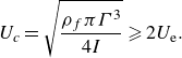 \begin{equation} U_c = \sqrt {\frac {\rho _f \pi \Gamma ^3}{4I}} \geqslant 2U_{\text{e}}. \end{equation}
Here, all variables are defined as described in § 3.2. Figure 15(a) shows $U_c$
compared with
$U_c$
compared with $2U_{e}$
. As shown in (a), the primary ring is expected to pinch-off at
$2U_{e}$
. As shown in (a), the primary ring is expected to pinch-off at $t_{pinch} = 0.33 t/t_{cycle} = 1 sec$
, when
$t_{pinch} = 0.33 t/t_{cycle} = 1 sec$
, when $U_{c}$
surpasses
$U_{c}$
surpasses $2U_{e}$
. We confirm this prediction by calculating the pLCS and nLCS ridges in the FTLE field in this time frame to show material boundaries indicative of pinch-off (Shadden et al. Reference Shadden, Dabiri and Marsden2006). In figures 16(a)–16(c), a closed LCS loop from overlaying the nFTLE and pFTLE fields is shown, indicating a pinched off vortex ring after the predicted
$2U_{e}$
. We confirm this prediction by calculating the pLCS and nLCS ridges in the FTLE field in this time frame to show material boundaries indicative of pinch-off (Shadden et al. Reference Shadden, Dabiri and Marsden2006). In figures 16(a)–16(c), a closed LCS loop from overlaying the nFTLE and pFTLE fields is shown, indicating a pinched off vortex ring after the predicted $t_{pinch}$
. As vortex ring pinch-off isn’t an instantaneous process, the additional time steps shown at
$t_{pinch}$
. As vortex ring pinch-off isn’t an instantaneous process, the additional time steps shown at $t=1.5t_{pinch}$
and
$t=1.5t_{pinch}$
and $t=3.75t_{pinch}$
in figures 16(b) and 16(c) provide additional insight that a single vortex structure is formed with a closed material boundary from the nLCS. As time progresses for
$t=3.75t_{pinch}$
in figures 16(b) and 16(c) provide additional insight that a single vortex structure is formed with a closed material boundary from the nLCS. As time progresses for ${L}/{D}=4$
, additional vorticity is produced and SV structures form in the wake of the PV. However, the primary closed loop of vorticity continues to travel downward without gaining additional fluid from the trailing jet formed in its wake, indicating an accurate prediction of
${L}/{D}=4$
, additional vorticity is produced and SV structures form in the wake of the PV. However, the primary closed loop of vorticity continues to travel downward without gaining additional fluid from the trailing jet formed in its wake, indicating an accurate prediction of $t_{pinch}$
.
$t_{pinch}$
.
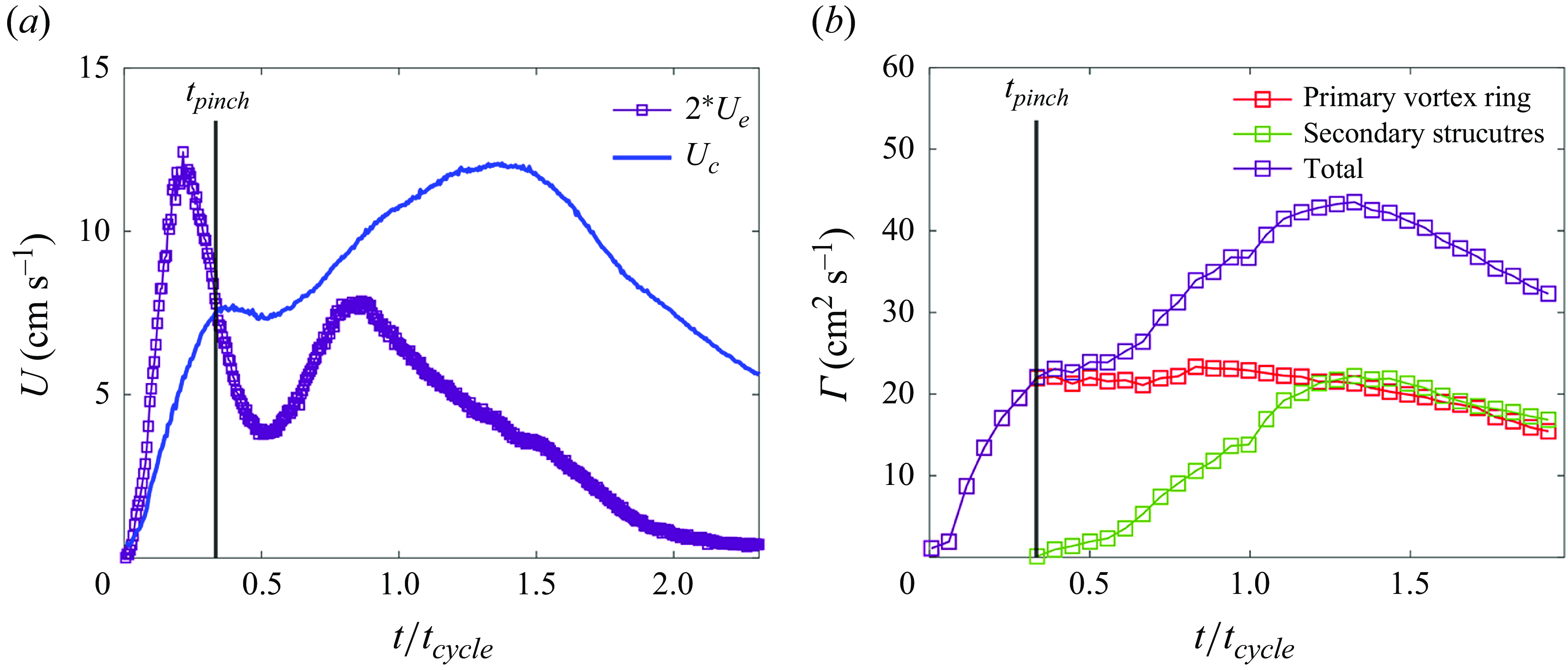
Figure 15. Predicting PV pinch-off for $Eh=29\,\rm N\,m^-{^1}$
,
$Eh=29\,\rm N\,m^-{^1}$
, ${L}/{D}=4$
. (a) Temporal evolution of
${L}/{D}=4$
. (a) Temporal evolution of $U_c$
and
$U_c$
and $2U_e$
to predict PV pinch-off when
$2U_e$
to predict PV pinch-off when $U_c\gt 2U_e$
(
$U_c\gt 2U_e$
( $t_{pinch}=0.33t/t_{cycle}\approx {1.0}$
sec). (b) Circulation contributions from PV and SV, calculated using the vorticity contours informed by the nLCS and pLCS.
$t_{pinch}=0.33t/t_{cycle}\approx {1.0}$
sec). (b) Circulation contributions from PV and SV, calculated using the vorticity contours informed by the nLCS and pLCS.
Through examining FTLE fields for each case within the studied parameter space, we can confirm closed off structures within the flow field. With this information, the vorticity fields measured directly from PIV can be used to separate the total circulation produced by each nozzle into the PV ring and the trailing jet formed in its wake. Figures 16(d)–16(e) show vorticity contours at the same instants as the FTLE fields in figures 16(a)–16(c), which are used to delineate circulation into separate parts of the flow, as informed by closed LCS contours in the FTLE field.
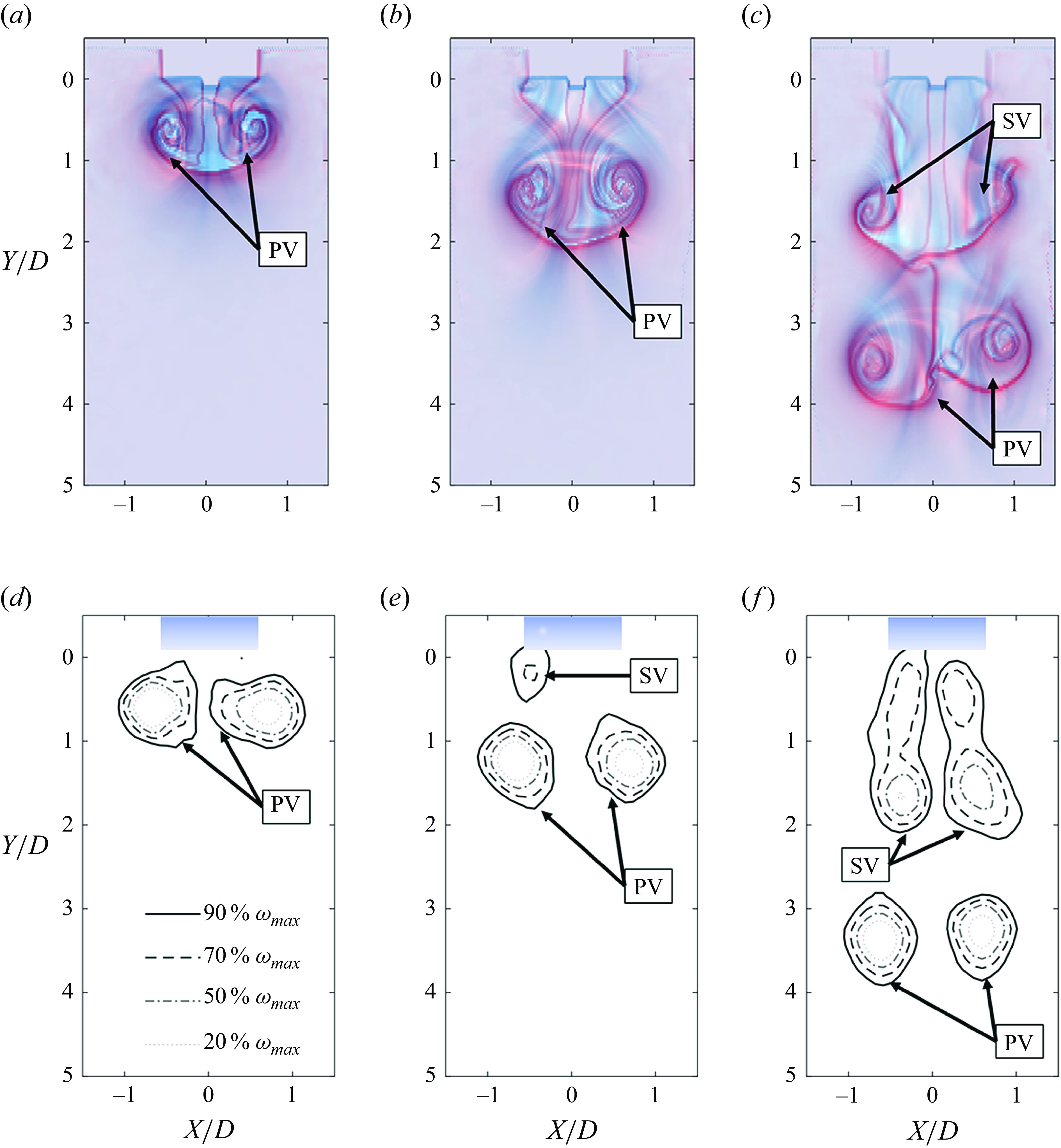
Figure 16. The FTLE fields and vorticity plots from the $Eh=29\,\rm N\,m^-{^1}$
nozzle with
$Eh=29\,\rm N\,m^-{^1}$
nozzle with ${L}/{D}=4$
. The red contours show attractive pLCS, and the blue contours show repelling nLCS: (a) nLCS and pLCS for
${L}/{D}=4$
. The red contours show attractive pLCS, and the blue contours show repelling nLCS: (a) nLCS and pLCS for $t=t_{pinch}$
; (b) nLCS and pLCS for
$t=t_{pinch}$
; (b) nLCS and pLCS for $t=1.5t_{pinch}$
; (c) nLCS and pLCS for
$t=1.5t_{pinch}$
; (c) nLCS and pLCS for $t=3.75t_{pinch}$
; (d–e) vorticity contours corresponding to the same time steps as the FTLE plots directly above each frame.
$t=3.75t_{pinch}$
; (d–e) vorticity contours corresponding to the same time steps as the FTLE plots directly above each frame.
Figure 15(b) shows the circulation contributions from the PV and SV structures and their sum of total circulation for $Eh = 29\,\rm N\,m^-{^1}$
. By informing the vorticity calculation through the use of the FTLE fields, the circulation from separate parts of the flow were confidently calculated without question as to whether or not vorticity was included from the trailing jet when calculating circulation for the PV and vice versa. As expected, the PV does not gain additional vorticity after the predicted
$Eh = 29\,\rm N\,m^-{^1}$
. By informing the vorticity calculation through the use of the FTLE fields, the circulation from separate parts of the flow were confidently calculated without question as to whether or not vorticity was included from the trailing jet when calculating circulation for the PV and vice versa. As expected, the PV does not gain additional vorticity after the predicted $t_{pinch}$
. Interestingly, the PV contains approximately 50 % of the total circulation produced, while the piston has only moved
$t_{pinch}$
. Interestingly, the PV contains approximately 50 % of the total circulation produced, while the piston has only moved ${1}/{3}$
of its total prescribed motion for
${1}/{3}$
of its total prescribed motion for ${L}/{D} = 4$
. This highlights that the benefits of utilising a flexible nozzle are most pronounced at a low ejected volume as there is a relatively diminished return in total circulation for the latter
${L}/{D} = 4$
. This highlights that the benefits of utilising a flexible nozzle are most pronounced at a low ejected volume as there is a relatively diminished return in total circulation for the latter ${2}/{3}$
of the piston motion, even though the piston travels a greater distance after the PV has pinched off. Additionally, for the
${2}/{3}$
of the piston motion, even though the piston travels a greater distance after the PV has pinched off. Additionally, for the $Eh=29\,\rm N\,m^-{^1}$
nozzle
$Eh=29\,\rm N\,m^-{^1}$
nozzle ${L}/{D}=1$
,
${L}/{D}=1$
, $t_{pinch} \approx t_{cycle}$
, indicating that the pump turns off when the PV exceeds the feeding velocity. In turn, this optimises the ejected volume by entraining the maximum vorticity within the PV, while minimising the piston motion. In figure 17(a) we compare the PV circulation measured from each ejected volume for the
$t_{pinch} \approx t_{cycle}$
, indicating that the pump turns off when the PV exceeds the feeding velocity. In turn, this optimises the ejected volume by entraining the maximum vorticity within the PV, while minimising the piston motion. In figure 17(a) we compare the PV circulation measured from each ejected volume for the $Eh = 29\,\rm N\,m^-{^1}$
nozzle and despite multiple vortex structures forming for
$Eh = 29\,\rm N\,m^-{^1}$
nozzle and despite multiple vortex structures forming for ${L}/{D} = 2, 4$
, we confirm that the PV strength (
${L}/{D} = 2, 4$
, we confirm that the PV strength ( $\Gamma _{PV}$
) does not grow with additional ejected volume beyond
$\Gamma _{PV}$
) does not grow with additional ejected volume beyond ${L}/{D} = 1$
. Given the exit (escape) velocity (
${L}/{D} = 1$
. Given the exit (escape) velocity ( $U_e$
) measured for each nozzle is approximately constant for
$U_e$
) measured for each nozzle is approximately constant for $t/t_{pinch}\lt 1$
we expect to find similar pinch-off results from varied
$t/t_{pinch}\lt 1$
we expect to find similar pinch-off results from varied ${L}/{D}$
.
${L}/{D}$
.
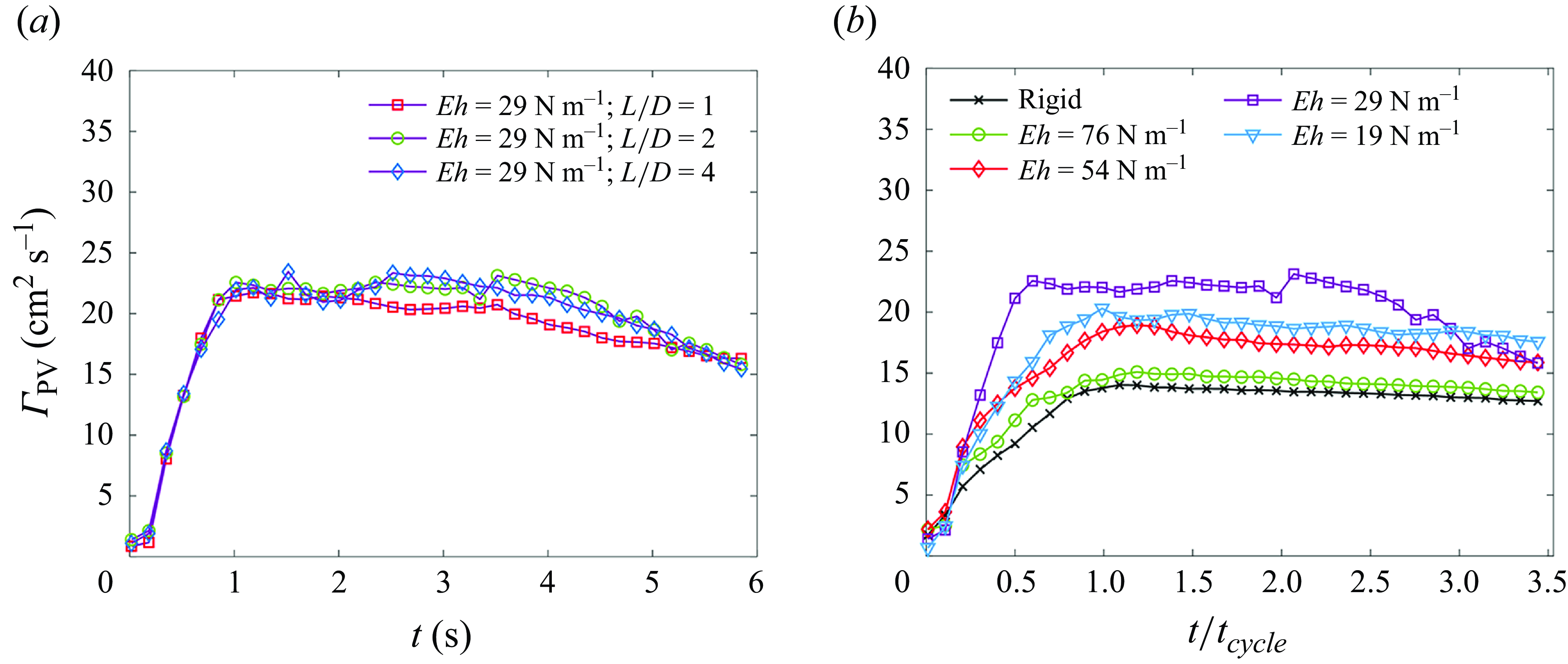
Figure 17. Primary vortex circulation. (a) Temporal development of only the PV circulation for all ${L}/{D}$
values generated with the
${L}/{D}$
values generated with the $Eh=29\,\rm N\,m^-{^1}$
nozzle. (b) Temporal development of PV circulation from each
$Eh=29\,\rm N\,m^-{^1}$
nozzle. (b) Temporal development of PV circulation from each $Eh$
nozzle for
$Eh$
nozzle for ${L}/{D}=2$
.
${L}/{D}=2$
.
This process was repeated for each nozzle and the vorticity contained within the PV as $Eh$
is varied follows the same trend as total circulation as shown in figure 13(b). The temporal variation of circulation measured for each of the PV cores produced by each nozzle from
$Eh$
is varied follows the same trend as total circulation as shown in figure 13(b). The temporal variation of circulation measured for each of the PV cores produced by each nozzle from ${L}/{D}=2$
is plotted in figure 17(b). One point to note is that the
${L}/{D}=2$
is plotted in figure 17(b). One point to note is that the $Eh = 19\,\rm N\,m^-{^1}$
PV pinches off significantly later than
$Eh = 19\,\rm N\,m^-{^1}$
PV pinches off significantly later than $Eh = 29\,\rm N\,m^-{^1}$
, as shown by the prolonged increased in circulation; however, the circulation contained within the PV is lower due to the lack of momentum flux (exit velocity) compared with the
$Eh = 29\,\rm N\,m^-{^1}$
, as shown by the prolonged increased in circulation; however, the circulation contained within the PV is lower due to the lack of momentum flux (exit velocity) compared with the $Eh =29\,\rm N\,m^-{^1}$
nozzle. The
$Eh =29\,\rm N\,m^-{^1}$
nozzle. The $Eh=29\,\rm N\,m^-{^1}$
nozzle creates the strongest PV, and further explains why the high non-dimensionalised impulse is reached for
$Eh=29\,\rm N\,m^-{^1}$
nozzle creates the strongest PV, and further explains why the high non-dimensionalised impulse is reached for ${L}/{D}=1$
, as the pump turns off immediately following PV pinch-off maximising the gain from pressure impulse. However, there is a very weak secondary structure formed for
${L}/{D}=1$
, as the pump turns off immediately following PV pinch-off maximising the gain from pressure impulse. However, there is a very weak secondary structure formed for $Eh = 29\,\rm N\,m^-{^1}$
,
$Eh = 29\,\rm N\,m^-{^1}$
, ${L}/{D}=1$
, when the nozzle collapses after
${L}/{D}=1$
, when the nozzle collapses after $t_{cycle}$
, yet the strength of this structure is very small and almost the entirety of the ejected fluid is contained within the PV.
$t_{cycle}$
, yet the strength of this structure is very small and almost the entirety of the ejected fluid is contained within the PV.
3.4. Stopping vortex formation and implications for bio-propulsors
To provide a complete picture of an entire cycle of the movement of the flexible nozzles, we investigate the flow structure produced by the nozzles reopening after collapse. Given that the nozzles were manufactured using clear silicone, we can perform PIV within the structure of the flexible nozzles (Choi & Park Reference Choi and Park2022). As described in § 3.1, the less stiff nozzles ( $Eh = 54, 29, 19\,\rm N\,m^-{^1}$
) collapse due to a pressure change at the outlet after the pump stops moving at
$Eh = 54, 29, 19\,\rm N\,m^-{^1}$
) collapse due to a pressure change at the outlet after the pump stops moving at $t_{cycle}$
. This is in contrast to the low pressure region formed within rigid nozzles upon fluid deceleration causing a decrease in pressure impulse (Gao et al. Reference Gao, Wang, Yu and Chyu2020). The flexible nozzles compliantly deform when this negative pressure gradient is formed and as a result see no loss in impulse as would be characterised by a slight dip in hydrodynamic impulse (Krueger & Gharib Reference Krueger and Gharib2005). After collapse, the nozzles reopen at time
$t_{cycle}$
. This is in contrast to the low pressure region formed within rigid nozzles upon fluid deceleration causing a decrease in pressure impulse (Gao et al. Reference Gao, Wang, Yu and Chyu2020). The flexible nozzles compliantly deform when this negative pressure gradient is formed and as a result see no loss in impulse as would be characterised by a slight dip in hydrodynamic impulse (Krueger & Gharib Reference Krueger and Gharib2005). After collapse, the nozzles reopen at time $t_{open}$
causing a suction velocity, which creates a stopping vortex of varied strength within the nozzle itself, similar to stopping vortices found in rigid nozzles that positively contribute to pressure impulse (Gao et al. Reference Gao, Wang, Yu and Chyu2020). The time to reach
$t_{open}$
causing a suction velocity, which creates a stopping vortex of varied strength within the nozzle itself, similar to stopping vortices found in rigid nozzles that positively contribute to pressure impulse (Gao et al. Reference Gao, Wang, Yu and Chyu2020). The time to reach $t_{open}$
is 0.95 s after
$t_{open}$
is 0.95 s after $t_{cycle}$
for
$t_{cycle}$
for $Eh=54\,\rm N\,m^-{^1}$
, whereas
$Eh=54\,\rm N\,m^-{^1}$
, whereas $t_{open}$
does not occur until 9 and 25 s after
$t_{open}$
does not occur until 9 and 25 s after $t_{cycle}$
for
$t_{cycle}$
for $Eh = 29$
and
$Eh = 29$
and $19\,\rm N\,m^-{^1}$
, respectively. Additionally, the time for the nozzles to fully refill (
$19\,\rm N\,m^-{^1}$
, respectively. Additionally, the time for the nozzles to fully refill ( $t_{refill}$
) (the time at which the circulation of the stopping vortex is the highest), is delayed with decreased nozzle stiffness. A summary of these time scales is shown in table 2 and figure 20(b) shows the nonlinear increase of
$t_{refill}$
) (the time at which the circulation of the stopping vortex is the highest), is delayed with decreased nozzle stiffness. A summary of these time scales is shown in table 2 and figure 20(b) shows the nonlinear increase of $t_{refill}$
as
$t_{refill}$
as $Eh$
is varied. Given that the
$Eh$
is varied. Given that the $Eh = 76\,\rm N\,m^-{^1}$
nozzle does not collapse, it does not produce a strong stopping vortex within the nozzle interior, and is not included in this stopping vortex analysis. It should be noted that whilst both the
$Eh = 76\,\rm N\,m^-{^1}$
nozzle does not collapse, it does not produce a strong stopping vortex within the nozzle interior, and is not included in this stopping vortex analysis. It should be noted that whilst both the $Eh = 76\,\rm N\,m^-{^1}$
and rigid nozzles do generate a beneficial stopping vortex below the nozzle exit after fluid deceleration is complete, it is very weak compared with the stopping vortex generated by the nozzles that collapsed and is outside the nozzle itself.
$Eh = 76\,\rm N\,m^-{^1}$
and rigid nozzles do generate a beneficial stopping vortex below the nozzle exit after fluid deceleration is complete, it is very weak compared with the stopping vortex generated by the nozzles that collapsed and is outside the nozzle itself.
Table 2. Nozzle reopening time scales.
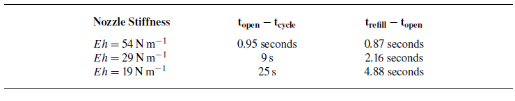
In terms of total momentum produced, forming stronger stopping vortices within the nozzle can increase the thrust of a bio-inspired propulsor, due to increased forward momentum within the nozzle itself (Xiaobo et al. Reference Xiaobo, Wei, Qiang and Jun2021). It has been demonstrated that for the swimming performance of siphonophores, animals that propel themselves with cyclical jets with refill cycles, the refill phase augments their distance travelled by 17 % over theoretical results which only generate thrust from the jet phase (Sutherland et al. Reference Sutherland, Gemmell, Colin and Costello2019). As the fluid accelerates back into the siphonophore, or in our case the nozzle, it generates a high pressure region that should augment thrust. Thus, quantifying this stopping vortex is imperative, in terms of summing the total thrust produced by our varied flexibility nozzles. Returning to jet propelled aquatic animals such as jellyfish and squid, they primarily produce forward momentum in the expelling cycle of their motion, but their swimming efficiency is linked to the generation of positive momentum in the refilling cycle known as passive energy recapture (Gemmell et al. Reference Gemmell, Colin and Costello2018). The locomotion of jellyfish particularly is significantly augmented by the presence of a stopping vortex which can account for up to 50 % of the jellyfish’s travel per cycle (Gemmell et al. Reference Gemmell, Costello, Colin, Stewart, Dabiri, Tafti and Priya2013).
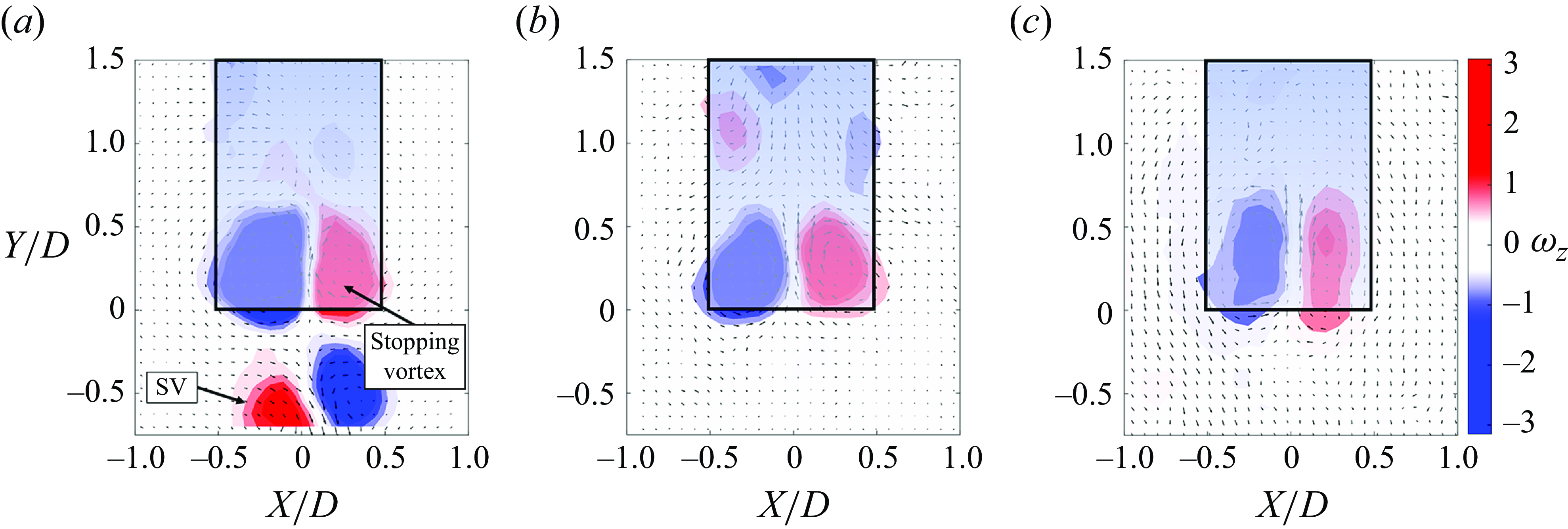
Figure 18. Stopping vortices produced varied $Eh$
nozzles at
$Eh$
nozzles at $t=0.75(t_{refill}-t_{open})$
. (a) Shows
$t=0.75(t_{refill}-t_{open})$
. (a) Shows $Eh = 54\,\rm N\,m^-{^1}$
. Note that the
$Eh = 54\,\rm N\,m^-{^1}$
. Note that the $Eh=54\,\rm N\,m^-{^1}$
nozzle immediately reopens, and thus there is secondary vorticity labelled in the frame, separate from the stopping vortex. Only vorticity contained within the stopping vortex is included for the circulation calculation. (b) Shows
$Eh=54\,\rm N\,m^-{^1}$
nozzle immediately reopens, and thus there is secondary vorticity labelled in the frame, separate from the stopping vortex. Only vorticity contained within the stopping vortex is included for the circulation calculation. (b) Shows $Eh = 29\,\rm N\,m^-{^1}$
and (c)
$Eh = 29\,\rm N\,m^-{^1}$
and (c) $Eh = 19\,\rm N\,m^-{^1}$
.
$Eh = 19\,\rm N\,m^-{^1}$
.
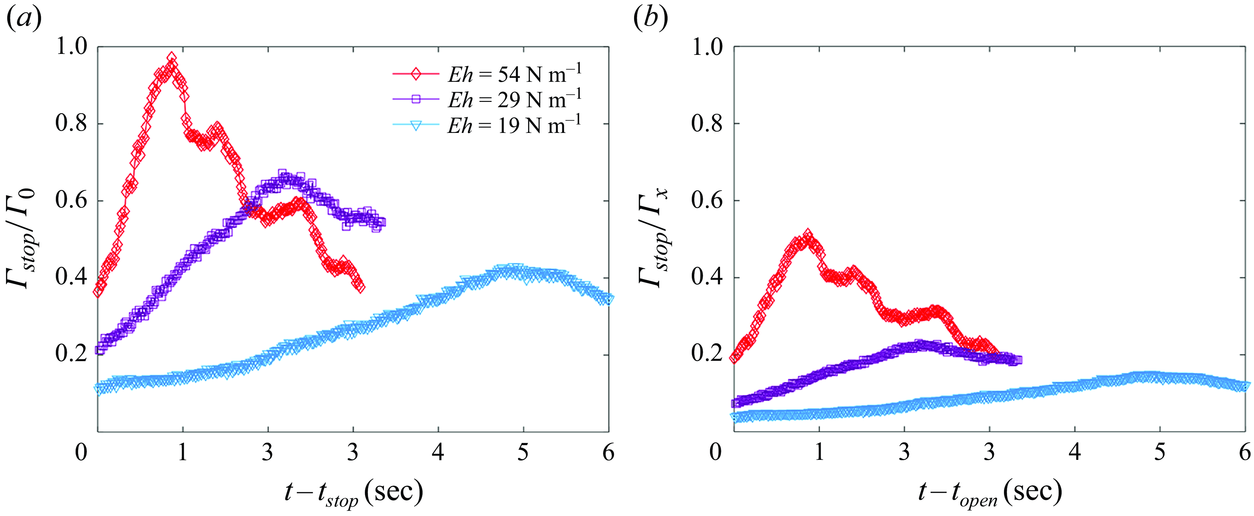
Figure 19. Circulation produced by the stopping vortices formed within the $Eh = 54, 29,$
and
$Eh = 54, 29,$
and $19\,\rm N\,m^-{^1}$
nozzles after
$19\,\rm N\,m^-{^1}$
nozzles after $t_{open}$
; (a)
$t_{open}$
; (a) ${\Gamma _{stop}}/{\Gamma _{0}}|_{t/t_{cycle}=1}$
, (b)
${\Gamma _{stop}}/{\Gamma _{0}}|_{t/t_{cycle}=1}$
, (b) ${\Gamma _{stop}}/{\Gamma _{x}}$
. Legend is the same for (a) and (b).
${\Gamma _{stop}}/{\Gamma _{x}}$
. Legend is the same for (a) and (b).
Figures 18(a)–18(c) show stopping vortices forming in the interior of the flexible $Eh=54, 29$
and
$Eh=54, 29$
and $19\,\rm N\,m^-{^1}$
nozzles at
$19\,\rm N\,m^-{^1}$
nozzles at $t=0.75(t_{refill}-t_{open})$
, or the time at which the stopping vortex has reached 75 % of the maximum
$t=0.75(t_{refill}-t_{open})$
, or the time at which the stopping vortex has reached 75 % of the maximum $\Gamma _{stop}$
. The strength of these stopping vortices is calculated using the circulation formulation described in § 3.3 and the temporal variation is plotted in figures 19(a) and 19(b). In figure 19(a)
$\Gamma _{stop}$
. The strength of these stopping vortices is calculated using the circulation formulation described in § 3.3 and the temporal variation is plotted in figures 19(a) and 19(b). In figure 19(a) ${\Gamma _{stop}}/{\Gamma _{0}}|_{t/t_{cycle}=1}$
is plotted, where
${\Gamma _{stop}}/{\Gamma _{0}}|_{t/t_{cycle}=1}$
is plotted, where $\Gamma _0$
is the circulation produced by the rigid nozzle throughout fluid expulsion for
$\Gamma _0$
is the circulation produced by the rigid nozzle throughout fluid expulsion for ${L}/{D}=1$
. This normalisation is selected to illustrate the importance of accounting for these stopping vortices relative to the circulation generated by the rigid nozzle. In figure 19(b)
${L}/{D}=1$
. This normalisation is selected to illustrate the importance of accounting for these stopping vortices relative to the circulation generated by the rigid nozzle. In figure 19(b) ${\Gamma _{stop}}/{\Gamma _{x}}$
is plotted where
${\Gamma _{stop}}/{\Gamma _{x}}$
is plotted where $\Gamma _x$
is the maximum circulation achieved by each respective flexible nozzle in expelling fluid for
$\Gamma _x$
is the maximum circulation achieved by each respective flexible nozzle in expelling fluid for ${L}/{D}=1$
. Note that the bounding area for the stopping vortex calculation was altered such that vorticity more than
${L}/{D}=1$
. Note that the bounding area for the stopping vortex calculation was altered such that vorticity more than $0.1D$
below the nozzle tip was not included in the calculation to avoid including vorticity produced in the jetting phase for the
$0.1D$
below the nozzle tip was not included in the calculation to avoid including vorticity produced in the jetting phase for the $54\,\rm N\,m^-{^1}$
nozzle as this nozzle starts to form stopping vortices rapidly after jetting. Additionally, measurements were cut off at
$54\,\rm N\,m^-{^1}$
nozzle as this nozzle starts to form stopping vortices rapidly after jetting. Additionally, measurements were cut off at $t-t_{open} = 3$
s, for
$t-t_{open} = 3$
s, for $Eh = 29$
and
$Eh = 29$
and $54\,\rm N\,m^-{^1}$
, due to the earlier occurrence of maximum
$54\,\rm N\,m^-{^1}$
, due to the earlier occurrence of maximum $\Gamma _{stop}$
. Alternatively, measurements were continued to
$\Gamma _{stop}$
. Alternatively, measurements were continued to $t - t_{open}=6$
s for the much slower reopening
$t - t_{open}=6$
s for the much slower reopening $Eh=19\,\rm N\,m^-{^1}$
nozzle. The strength of the stopping vortex scales with the stiffness of the collapsing flexible nozzles with the
$Eh=19\,\rm N\,m^-{^1}$
nozzle. The strength of the stopping vortex scales with the stiffness of the collapsing flexible nozzles with the $Eh = 54\,\rm N\,m^-{^1}$
nozzle creating the strongest and
$Eh = 54\,\rm N\,m^-{^1}$
nozzle creating the strongest and $Eh = 19\,\rm N\,m^-{^1}$
generating the weakest, as the stiffer nozzle reopens much faster, i.e. shorter
$Eh = 19\,\rm N\,m^-{^1}$
generating the weakest, as the stiffer nozzle reopens much faster, i.e. shorter $t_{refill}$
, generating a stronger stopping vortex. The strength of the vortex is not affected by
$t_{refill}$
, generating a stronger stopping vortex. The strength of the vortex is not affected by ${L}/{D}$
as the same initial condition is provided to each nozzle at the end of flow generation with the same deceleration of fluid, or pressure change resulting in a collapsed nozzle shape.
${L}/{D}$
as the same initial condition is provided to each nozzle at the end of flow generation with the same deceleration of fluid, or pressure change resulting in a collapsed nozzle shape.
Figure 20(a) shows the maximum stopping vortex strength ( $\Gamma _{stop}$
) for each nozzle stiffness alongside the maximum total circulation generating while expelling fluid (
$\Gamma _{stop}$
) for each nozzle stiffness alongside the maximum total circulation generating while expelling fluid ( $\Gamma _{expulsion}$
) at
$\Gamma _{expulsion}$
) at ${L}/{D} = 1$
, normalised by the maximum rigid nozzle circulation (
${L}/{D} = 1$
, normalised by the maximum rigid nozzle circulation ( $\Gamma _0$
) at
$\Gamma _0$
) at ${L}/{D} = 1$
. Here,
${L}/{D} = 1$
. Here, $\Gamma _{stop}$
is averaged across all
$\Gamma _{stop}$
is averaged across all ${L}/{D}$
, as there is negligible difference between the strength of the vortices produced with
${L}/{D}$
, as there is negligible difference between the strength of the vortices produced with $L/D$
(nozzle starts with the same, collapsed initial condition for all
$L/D$
(nozzle starts with the same, collapsed initial condition for all $L/D$
; changing the ejected volume did not alter the nozzle reopening rate). As shown in figure 20(a), the
$L/D$
; changing the ejected volume did not alter the nozzle reopening rate). As shown in figure 20(a), the $Eh = 54\,\rm N\,m^-{^1}$
nozzle produced the strongest stopping vortex, whereas the other nozzles either do not collapse (
$Eh = 54\,\rm N\,m^-{^1}$
nozzle produced the strongest stopping vortex, whereas the other nozzles either do not collapse ( $Eh = 76\,\rm N\,m^-{^1}$
) or reopen slowly after collapse (
$Eh = 76\,\rm N\,m^-{^1}$
) or reopen slowly after collapse ( $Eh = 29$
and
$Eh = 29$
and $19\,\rm N\,m^-{^1}$
), resulting in weaker stopping vortices. Notably, the peak for
$19\,\rm N\,m^-{^1}$
), resulting in weaker stopping vortices. Notably, the peak for $\Gamma _{stop}$
does not align with the peak (optimal nozzle stiffness for increased expulsion circulation) for
$\Gamma _{stop}$
does not align with the peak (optimal nozzle stiffness for increased expulsion circulation) for $\Gamma _{expulsion}$
. This suggests that the full-cycle can be further optimised in the case of pulsed vortex rings (maximum circulation generated in both expulsion and in stopping) by ensuring these peaks align.
$\Gamma _{expulsion}$
. This suggests that the full-cycle can be further optimised in the case of pulsed vortex rings (maximum circulation generated in both expulsion and in stopping) by ensuring these peaks align.
However, in addition to the vortex strength, consideration must also be given to the time for the nozzle to finish refilling after the expulsion process (i.e. completely generate the stopping vortex and return to initial open state). It is noted that the time to refill ( $t_{refill} - t_{cycle}$
) for
$t_{refill} - t_{cycle}$
) for $Eh = 29\,\rm N\,m^-{^1}$
is six times longer than the
$Eh = 29\,\rm N\,m^-{^1}$
is six times longer than the $Eh = 54\,\rm N\,m^-{^1}$
nozzle. As the propulsive benefits of the flexible nozzle depend on its initial open starting condition (to ensure maximum inward deflection during vortex ring expulsion), it is important that the nozzle return to this state quickly to begin the next vortex expulsion cycle. Although the
$Eh = 54\,\rm N\,m^-{^1}$
nozzle. As the propulsive benefits of the flexible nozzle depend on its initial open starting condition (to ensure maximum inward deflection during vortex ring expulsion), it is important that the nozzle return to this state quickly to begin the next vortex expulsion cycle. Although the $Eh = 29\,\rm N\,m^-{^1}$
nozzle may outperform the other nozzles during the expulsion process in the present study, the
$Eh = 29\,\rm N\,m^-{^1}$
nozzle may outperform the other nozzles during the expulsion process in the present study, the $Eh = 54\,\rm N\,m^-{^1}$
nozzle would likely be more applicable to a bio-inspired propulsor as the time to complete a expulsion–refill cycle is greatly reduced. This highlights the importance of tuning the acceleration of the fluid with the damped natural frequency of the stiffest nozzle that will still collapse under deceleration to generate a strong PV ring, a strong stopping vortex and all within a relatively short duration.
$Eh = 54\,\rm N\,m^-{^1}$
nozzle would likely be more applicable to a bio-inspired propulsor as the time to complete a expulsion–refill cycle is greatly reduced. This highlights the importance of tuning the acceleration of the fluid with the damped natural frequency of the stiffest nozzle that will still collapse under deceleration to generate a strong PV ring, a strong stopping vortex and all within a relatively short duration.
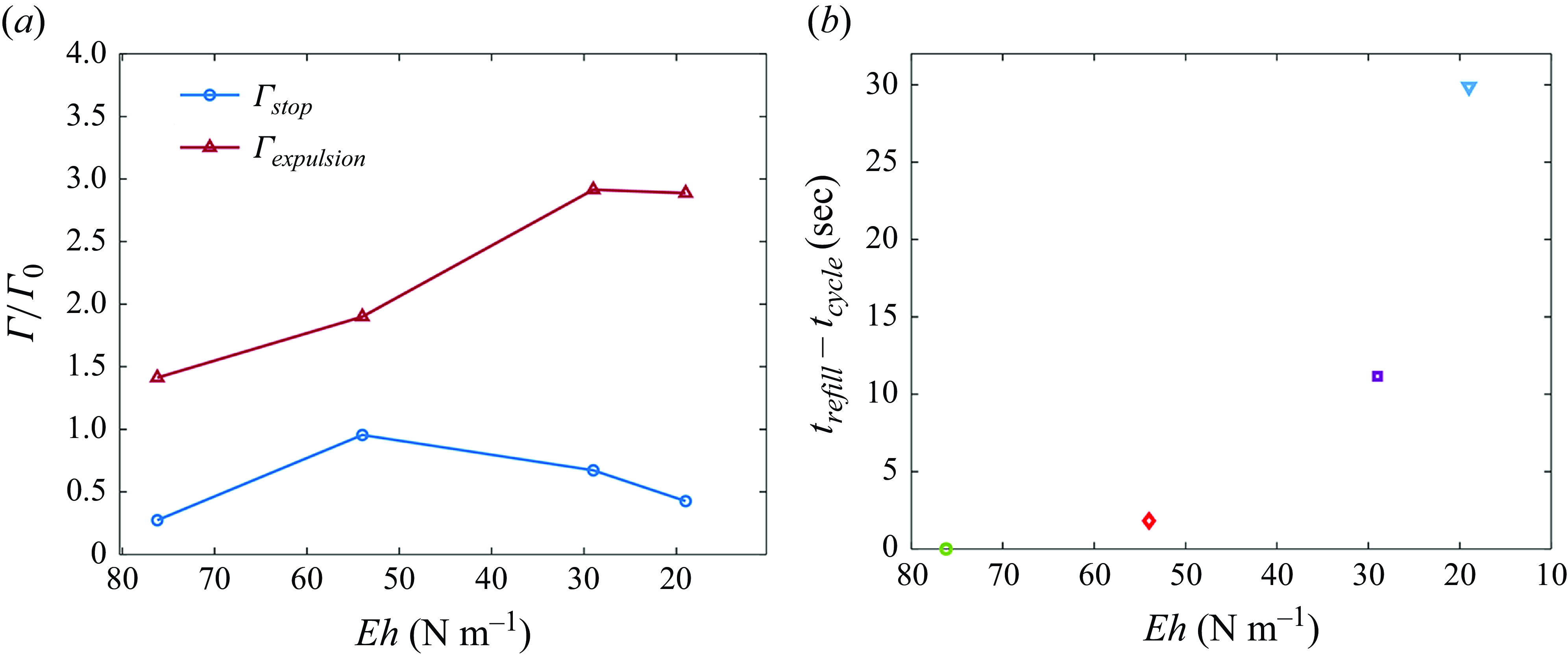
Figure 20. Circulation and time for the flexible nozzles to fully reopen; (a) $\Gamma _{stop}/\Gamma _{0}$
averaged across all
$\Gamma _{stop}/\Gamma _{0}$
averaged across all ${L}/{D}$
values and
${L}/{D}$
values and $\Gamma _{expulsion}/\Gamma _{0}$
for
$\Gamma _{expulsion}/\Gamma _{0}$
for ${L}/{D}=1$
, (b)
${L}/{D}=1$
, (b) $t_{refill} - t_{cycle}$
, or time after the pump turns off for the nozzles to completely reopen generating the stopping vortex.
$t_{refill} - t_{cycle}$
, or time after the pump turns off for the nozzles to completely reopen generating the stopping vortex.
To summarise, the present study, in alignment with previous studies (Choi & Park Reference Choi and Park2022, Reference Choi and Park2024), indicates that the optimal stiffness nozzle in the jetting phase should have peak tip deformation synchronised with the input fluid acceleration for maximal momentum transfer. However, we also now observe that it is equally important that the nozzle reopens as quickly as possible during the refilling cycle, which adds a second condition to define the optimal nozzle stiffness for a complete expulsion–refill cycle. This secondary aspect of nozzle stiffness is characterised by a nozzle that is compliant enough to collapse from fluid deceleration, yet remains as stiff as possible to reopen quickly. Despite forming a stopping vortex, this is expected to benefit propulsion by creating net positive momentum and a favourable pressure gradient. This suggests that tuning the system ( $t_{acc}$
) to maximise the jetting conditions for the stiffest nozzle capable of collapse would generate the largest net thrust over a full expulsion-refill cycle by additionally forming the strongest stopping vortices.
$t_{acc}$
) to maximise the jetting conditions for the stiffest nozzle capable of collapse would generate the largest net thrust over a full expulsion-refill cycle by additionally forming the strongest stopping vortices.
4. Conclusions
In this work, the relative impulse generated by a flexible nozzle was found to be increased by up to 2.8 times compared with that of a rigid case with the same kinematic input to the nozzle. Similar to previous studies we find that decreasing stiffness past an optimal value results in a decline in measured output. The most flexible nozzle tested in this study was found to reduce the maximum measured circulation and impulse due to the nozzle’s damped frequency becoming too slow relative to the input fluid acceleration. Synchronising the timing at which the nozzle contracts with the end of the unperturbed fluid acceleration resulted in the optimal thrust conditions by timing the release of elastic energy (Choi & Park Reference Choi and Park2022, Reference Choi and Park2024). When these time scales align, the entirety of the elastic energy from the nozzle is imparted while the input fluid is accelerating achieving peak output velocities, resulting in the largest increase in circulation and impulse. Based on the optimal timing condition proposed by Choi & Park (Reference Choi and Park2022, Reference Choi and Park2024), an experimental method was developed to determine the optimal nozzle stiffness based on the measured damped natural frequency ( $\omega _d$
) of the nozzle via FFT. Once
$\omega _d$
) of the nozzle via FFT. Once $\omega _d$
is determined for a flexible nozzle, it can be used to predict the time at which the nozzle will deform inward, allowing for proper tuning of the fluid acceleration time from the pumping system. It is understood that this method utilising
$\omega _d$
is determined for a flexible nozzle, it can be used to predict the time at which the nozzle will deform inward, allowing for proper tuning of the fluid acceleration time from the pumping system. It is understood that this method utilising $\omega _d$
could be applied to a variety of flexible nozzle geometries for prediction of an optimal stiffness within a similar Reynolds number regime, and remains an avenue for future research. It is additionally observed that when these time scales are synchronised, the slight negative pressure from the change in input velocity and vortex formation generate a positive feedback loop wherein the optimal stiffness nozzle deformation is magnified. Alternatively, if the nozzle contracts too quickly or too slow relative to the input flow, there is only a modest increase in output velocity and impulse.
$\omega _d$
could be applied to a variety of flexible nozzle geometries for prediction of an optimal stiffness within a similar Reynolds number regime, and remains an avenue for future research. It is additionally observed that when these time scales are synchronised, the slight negative pressure from the change in input velocity and vortex formation generate a positive feedback loop wherein the optimal stiffness nozzle deformation is magnified. Alternatively, if the nozzle contracts too quickly or too slow relative to the input flow, there is only a modest increase in output velocity and impulse.
The lowest ejected volume, ${L}/{D}=1$
, generated the largest relative impulse due to the initial peak increase in fluid velocity from the nozzle elastic energy, minimising the negative pressure gradient in deceleration via nozzle collapse, a higher relative increase in
${L}/{D}=1$
, generated the largest relative impulse due to the initial peak increase in fluid velocity from the nozzle elastic energy, minimising the negative pressure gradient in deceleration via nozzle collapse, a higher relative increase in $({L}/{D})_{eff}$
, and the formation of a single coherent vortex structure. The combination of these factors results in the greatest measured hydrodynamic impulse by increasing the momentum flux (output velocity) and the pressure contribution through the formation of a single vortex ring while simultaneously suppressing the negative deceleration pressure gradient through nozzle collapse. For example, for a larger ejected volume of
$({L}/{D})_{eff}$
, and the formation of a single coherent vortex structure. The combination of these factors results in the greatest measured hydrodynamic impulse by increasing the momentum flux (output velocity) and the pressure contribution through the formation of a single vortex ring while simultaneously suppressing the negative deceleration pressure gradient through nozzle collapse. For example, for a larger ejected volume of ${L}/{D}=4$
and the optimal stiffness
${L}/{D}=4$
and the optimal stiffness $Eh=29\,\rm N\,m^-{^1}$
nozzle, the secondary structures contribute approximately half of the total circulation, while consuming 2/3 of the piston motion measured at the pump. It is also noted, that after the nozzle provides elastic energy to the flow, it extracts energy back from the fluid to reopen, decreasing the output velocity. For the lowest ejected volume, the pump turns off when the nozzle begins to re-expand, negating the need to overcome the counter-flow velocity generated in the re-expansion process, where higher ejected volumes continue to eject fluid to overcome this counter flow.
$Eh=29\,\rm N\,m^-{^1}$
nozzle, the secondary structures contribute approximately half of the total circulation, while consuming 2/3 of the piston motion measured at the pump. It is also noted, that after the nozzle provides elastic energy to the flow, it extracts energy back from the fluid to reopen, decreasing the output velocity. For the lowest ejected volume, the pump turns off when the nozzle begins to re-expand, negating the need to overcome the counter-flow velocity generated in the re-expansion process, where higher ejected volumes continue to eject fluid to overcome this counter flow.
In this study, we predict the vortex pinch-off time for each nozzle and find that the PV pinch-off is relatively unaffected by different ejected volumes for the optimal stiffness nozzle. This is due to a peak in output velocity which feeds the PV for a short time, but as the output velocity decreases due to the nozzle re-expanding, the PV outpaces the feeding velocity. The predicted pinch-off for the optimal material property nozzle, occurs at almost the exact time at which the pump stops moving for ${L}/{D}=1$
as measured at the pump. In turn, this generates the strongest possible single vortex ring for the provided input flow conditions which maximises the pressure contribution to hydrodynamic impulse. This is similar to previous work which has shown that hydrodynamic impulse from a rigid nozzle is maximised per unit volume via the pressure impulse contribution up to
${L}/{D}=1$
as measured at the pump. In turn, this generates the strongest possible single vortex ring for the provided input flow conditions which maximises the pressure contribution to hydrodynamic impulse. This is similar to previous work which has shown that hydrodynamic impulse from a rigid nozzle is maximised per unit volume via the pressure impulse contribution up to ${L}/{D}\approx 4$
when a single vortex ring without a trailing jet is formed (Krueger & Gharib Reference Krueger and Gharib2003).
${L}/{D}\approx 4$
when a single vortex ring without a trailing jet is formed (Krueger & Gharib Reference Krueger and Gharib2003).
For the most flexible nozzles ( $Eh = 54, 29, 19\,\rm N\,m^-{^1}$
), the fluid deceleration creates a negative pressure gradient causing varying nozzle collapse after
$Eh = 54, 29, 19\,\rm N\,m^-{^1}$
), the fluid deceleration creates a negative pressure gradient causing varying nozzle collapse after $t_{cycle}$
. When the nozzles reopen, they create a stopping vortex within the nozzle walls, which should theoretically positively contribute to the overall momentum of a free bodied system (Xiaobo et al. Reference Xiaobo, Wei, Qiang and Jun2021). The stopping vortex was maximised from the
$t_{cycle}$
. When the nozzles reopen, they create a stopping vortex within the nozzle walls, which should theoretically positively contribute to the overall momentum of a free bodied system (Xiaobo et al. Reference Xiaobo, Wei, Qiang and Jun2021). The stopping vortex was maximised from the $Eh=54\,\rm N\,m^-{^1}$
nozzle, due to relatively higher nozzle stiffness allowing for a much quicker reopening, yet it was still flexible enough to collapse under the negative pressure gradient upon fluid deceleration. This study highlights that the optimal nozzle condition for
$Eh=54\,\rm N\,m^-{^1}$
nozzle, due to relatively higher nozzle stiffness allowing for a much quicker reopening, yet it was still flexible enough to collapse under the negative pressure gradient upon fluid deceleration. This study highlights that the optimal nozzle condition for $\Gamma _{expulsion}$
is not necessarily the optimal nozzle condition for
$\Gamma _{expulsion}$
is not necessarily the optimal nozzle condition for $\Gamma _{stop}$
under a given input flow condition. Additionally, due to the extremely low stiffness of the
$\Gamma _{stop}$
under a given input flow condition. Additionally, due to the extremely low stiffness of the $Eh=29$
and
$Eh=29$
and $19\,\rm N\,m^-{^1}$
nozzles, they remain collapsed for 9 and 29 s, respectively, which would become significant in terms of optimising a pulsed jet flow. Further examination into a pulsed flow may result in the reduction of the propulsive benefit from these nozzles as they would be starting with a closed initial configuration which is a lower energetic state, as the elastic potential energy from the nozzle is not available as an initial condition. Overall, this work suggests that selecting a fluid acceleration time scale that matches the elastic properties of a flexible nozzle while still maintaining the most stiffness possible in the nozzle should theoretically create the maximum thrust per pulse based on the current study, to generate the most momentum impulse in the jetting phase and the strongest stopping vortex in the refilling phase.
$19\,\rm N\,m^-{^1}$
nozzles, they remain collapsed for 9 and 29 s, respectively, which would become significant in terms of optimising a pulsed jet flow. Further examination into a pulsed flow may result in the reduction of the propulsive benefit from these nozzles as they would be starting with a closed initial configuration which is a lower energetic state, as the elastic potential energy from the nozzle is not available as an initial condition. Overall, this work suggests that selecting a fluid acceleration time scale that matches the elastic properties of a flexible nozzle while still maintaining the most stiffness possible in the nozzle should theoretically create the maximum thrust per pulse based on the current study, to generate the most momentum impulse in the jetting phase and the strongest stopping vortex in the refilling phase.
Supplementary materials
Supplementary materials are available at https://doi.org/10.1017/jfm.2025.378.
Acknowledgements
The authors would like to thank Dr Y. Li, M. Ahsan Habib and N. Raventhiran (M-Left, Montana State University) for their assistance with nozzle wall thickness measurements and Dr S. Sofie (Montana State University) for his assistance with material tensile testing.
Funding
This research received no specific grant from any funding agency, commercial or not-for-profit sectors.
Declaration of interests
The authors report no conflict of interest.
Appendix A. Comparison of Circulation Generated in XY and YZ Planes
The following figures demonstrate the formation of a closed constant loop of vorticity from each of the flexible nozzles despite loss of axisymmetric shape upon nozzle collapse for the $Eh = 54, 29$
and
$Eh = 54, 29$
and $19\,\rm N\,m^-{^1}$
nozzles. The rigid nozzle and
$19\,\rm N\,m^-{^1}$
nozzles. The rigid nozzle and $Eh = 76\,\rm N\,m^-{^1}$
nozzle are not shown as there was no preferential axis of nozzle collapse for these nozzles. In figures 21, 22and 23, the circulation measured in the perpendicular XY and XZ planes are shown for the
$Eh = 76\,\rm N\,m^-{^1}$
nozzle are not shown as there was no preferential axis of nozzle collapse for these nozzles. In figures 21, 22and 23, the circulation measured in the perpendicular XY and XZ planes are shown for the $Eh = 54, 29$
and
$Eh = 54, 29$
and $19$
N/m nozzles, respectively.
$19$
N/m nozzles, respectively.
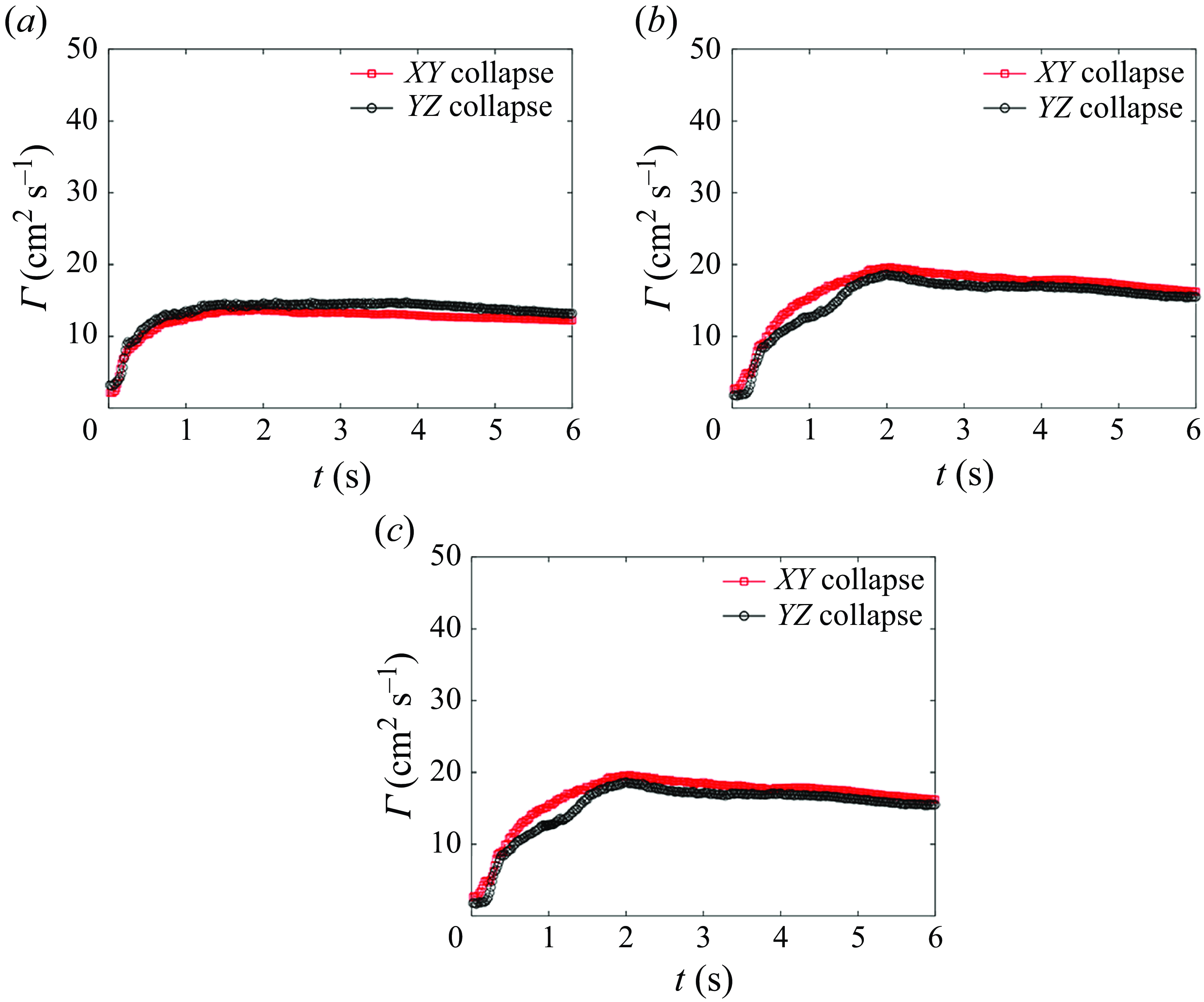
Figure 21. Circulation measured in the XY and XZ planes for the $Eh = 54$
N/m nozzle; (a)
$Eh = 54$
N/m nozzle; (a) ${L}/{D} = 1$
, (b)
${L}/{D} = 1$
, (b) ${L}/{D} = 2$
, (c)
${L}/{D} = 2$
, (c) ${L}/{D}=4$
.
${L}/{D}=4$
.
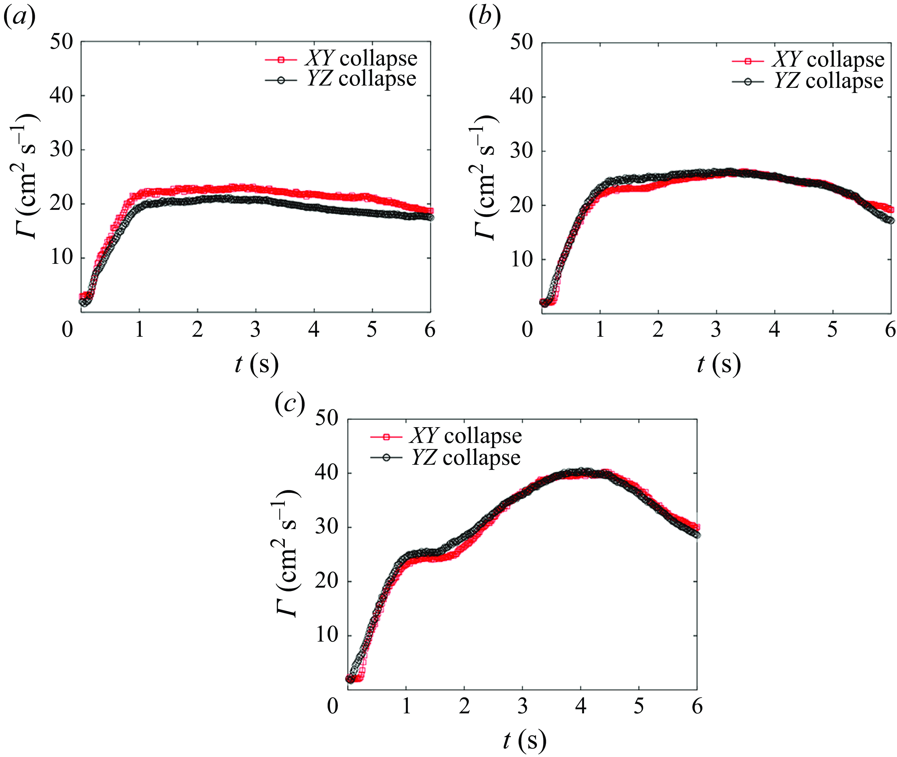
Figure 22. Circulation measured in the XY and XZ planes for the $Eh = 29$
N/m nozzle; (a)
$Eh = 29$
N/m nozzle; (a) ${L}/{D} = 1$
, (b)
${L}/{D} = 1$
, (b) ${L}/{D} = 2$
, (c)
${L}/{D} = 2$
, (c) ${L}/{D}=4$
.
${L}/{D}=4$
.
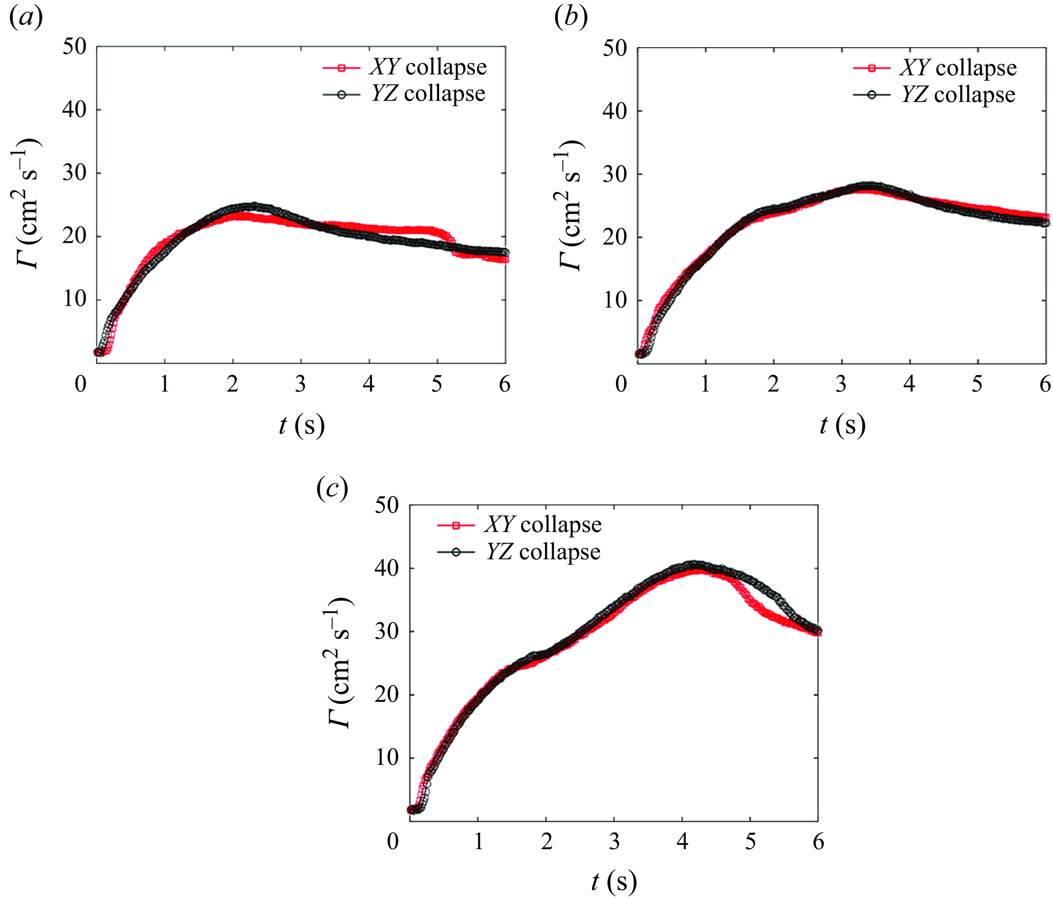
Figure 23. Circulation measured in the XY and XZ planes for the $Eh = 19$
N/m nozzle; (a)
$Eh = 19$
N/m nozzle; (a) ${L}/{D} = 1$
, (b)
${L}/{D} = 1$
, (b) ${L}/{D} = 2$
, (c)
${L}/{D} = 2$
, (c) ${L}/{D}=4$
.
${L}/{D}=4$
.


 Open access