


1. Introduction
Nonlinear dynamical systems often undergo state transitions as the control parameters are changed. Such bifurcations are generally characterised numerically using bifurcation diagrams. For example, to obtain steady and periodic solutions of nonlinear systems, numerical bifurcation analyses are performed in phase diagrams spanned by control parameters (Dijkstra et al. Reference Dijkstra2014); the continuation methods have been preferred to find these bifurcation diagrams, for example in thermal convection problems, such as in inclined layer convection (ILC) (Reetz & Schneider Reference Reetz and Schneider2020; Reetz, Subramanian & Schneider Reference Reetz, Subramanian and Schneider2020) and in steady planar Rayleigh–Bénard convection (RBC) with side-wall effects (Boullé et al. Reference Boullé, Dallas and Farrell2022). The bifurcation studies may also reveal junction points in bifurcation diagrams at which two or more branches of solutions intersect, implying the coexistence of several statistically stationary states with different transport properties for the same control parameters. Such bifurcation junctions have been reported in both turbulent and non-turbulent flow regimes. In recent literature, these states have been referred to as the multiple states. Examples of such flows include Taylor–Couette flow (Huisman et al. Reference Huisman, van der Veen, Sun and Lohse2014; van der Veen et al. Reference van der Veen, Huisman, Dung, Tang, Sun and Lohse2016), both rotating RBC and non-rotating two-dimensional (2-D) RBC (Xi & Xia Reference Xi and Xia2008; van der Poel et al. Reference van der Poel, Stevens, Sugiyama and Lohse2012; Wang et al. Reference Wang, Wan, Yan and Sun2018; Favier, Guervilly & Knobloch Reference Favier, Guervilly and Knobloch2019), double diffusive convection (Yang et al. Reference Yang, Chen, Verzicco and Lohse2020), rotating spherical Couette flow (Zimmerman, Triana & Lathrop Reference Zimmerman, Triana and Lathrop2011) and von Karman flow (Ravelet et al. Reference Ravelet, Marié, Chiffaudel and Daviaud2004; Cortet et al. Reference Cortet, Chiffaudel, Daviaud and Dubrulle2010; Faranda et al. Reference Faranda, Sato, Saint-Michel, Wiertel, Padilla, Dubrulle and Daviaud2017), as well as some geophysical flows (Broecker, Peteet & Rind Reference Broecker, Peteet and Rind1985; Weeks et al. Reference Weeks, Tian, Urbach, Ide, Swinney and Ghil1997; Schmeits & Dijkstra Reference Schmeits and Dijkstra2001; Li, Sato & Kageyama Reference Li, Sato and Kageyama2002). For discovering the multiple states without change in control parameters, scientists have relied on computer simulations designed to yield these states. In the present work, we present a simple yet efficient methodology to quickly uncover the possible multiple states for a chosen set of control parameters in the turbulent regime in an example flow configuration, i.e. 2-D RBC.
The RBC is a canonical flow configuration for thermal convection. Fluid entrapped between a heated bottom plate and a cooled top plate is driven by buoyancy in RBC (Bodenschatz, Pesch & Ahlers Reference Bodenschatz, Pesch and Ahlers2000; Ahlers, Grossmann & Lohse Reference Ahlers, Grossmann and Lohse2009; Chillà & Schumacher Reference Chillà and Schumacher2012; Schumacher & Sreenivasan Reference Schumacher and Sreenivasan2020; Xia et al. Reference Xia, Huang, Xie and Zhang2023; Lohse & Shishkina Reference Lohse and Shishkina2024). Generally, the effect of buoyancy is modelled using the Boussinesq approximation. Large-scale superstructures of horizontal size much larger than the distance between the plates are prevalent in three-dimensional (3-D) RBC (Pandey, Scheel & Schumacher Reference Pandey, Scheel and Schumacher2018; Stevens et al. Reference Stevens, Blass, Zhu, Verzicco and Lohse2018; Krug, Lohse & Stevens Reference Krug, Lohse and Stevens2020), and multiple states with different transport properties have not been identified as such. On the other hand, large-scale convection rolls whose horizontal size is similar to the distance between the plates are a distinctive feature of 2-D RBC. Depending on the flow driving strength, multiple roll states with different mean aspect ratios (
 $\Gamma _r$
) can be yielded. Wang et al. (Reference Wang, Verzicco, Lohse and Shishkina2020) extensively explored 2-D planar RBC over a wide range of Rayleigh numbers (
$\Gamma _r$
) can be yielded. Wang et al. (Reference Wang, Verzicco, Lohse and Shishkina2020) extensively explored 2-D planar RBC over a wide range of Rayleigh numbers (
 $10^7 \leqslant Ra \leqslant 10^{10}$
) and Prandtl numbers (
$10^7 \leqslant Ra \leqslant 10^{10}$
) and Prandtl numbers (
 $1 \leqslant Pr \leqslant 100$
) in computer simulations. They obtained multiple states with
$1 \leqslant Pr \leqslant 100$
) in computer simulations. They obtained multiple states with
 ${2}/{3} \leqslant \Gamma _r \leqslant {4}/{3}$
; the lower limit is approached at larger
${2}/{3} \leqslant \Gamma _r \leqslant {4}/{3}$
; the lower limit is approached at larger
 $Ra$
. They showed that the range of
$Ra$
. They showed that the range of
 $\Gamma _r$
obtained in simulations is reliant on the balance between elliptic instability and viscous damping.
$\Gamma _r$
obtained in simulations is reliant on the balance between elliptic instability and viscous damping.
The multiple states captured by Wang et al. (Reference Wang, Verzicco, Lohse and Shishkina2020) in their direct numerical simulations (DNS) depended on the aspect ratio of the initial roll states. In cases where
 $\Gamma _r$
of the converged statistically stationary state was different from the initial state, the convergence routes involved long transitions between states. In addition, the use of an exhaustive set of initial conditions for the realisation of all possible states might not be possible in such a methodology. Herein, we propose a novel technique that eliminates specific triad interactions involving one or more characteristic wavenumbers corresponding to the desired roll size. Consequently, roll formation at the target wavenumbers is suppressed, encouraging roll formation at other candidate wavenumbers. The proposed methodology can capture a state significantly quicker than even the DNS initialised with a target roll state, and the convergence route does not include state transitions. As will be demonstrated in the paper, this method circumvents the dependence of the converged roll state on the initial condition. The converged flow statistics obtained for the multiple states using the proposed method, such as Nusselt number (
$\Gamma _r$
of the converged statistically stationary state was different from the initial state, the convergence routes involved long transitions between states. In addition, the use of an exhaustive set of initial conditions for the realisation of all possible states might not be possible in such a methodology. Herein, we propose a novel technique that eliminates specific triad interactions involving one or more characteristic wavenumbers corresponding to the desired roll size. Consequently, roll formation at the target wavenumbers is suppressed, encouraging roll formation at other candidate wavenumbers. The proposed methodology can capture a state significantly quicker than even the DNS initialised with a target roll state, and the convergence route does not include state transitions. As will be demonstrated in the paper, this method circumvents the dependence of the converged roll state on the initial condition. The converged flow statistics obtained for the multiple states using the proposed method, such as Nusselt number (
 $Nu$
) and volume-averaged horizontal and vertical Reynolds numbers, are also found to be in very good agreement with those obtained from DNS.
$Nu$
) and volume-averaged horizontal and vertical Reynolds numbers, are also found to be in very good agreement with those obtained from DNS.
The turbulent 2-D RBC system allows for multiple states for a particular set of control parameters, unlike most other previous studies of emerging states in thermal convection with change in control parameters. For example, the bifurcation studies of ILC by Reetz & Schneider (Reference Reetz and Schneider2020) and Reetz et al. (Reference Reetz, Subramanian and Schneider2020) obtained the different states in phase diagrams changing the control parameters. In their ILC system, Reetz et al. (Reference Reetz, Subramanian and Schneider2020) found that (see p. 3 therein): ‘Complex temporal dynamics may be observed where invariant states coexist at equal values of the control parameters.’ In the present work, we compute these multiple states in a turbulent regime, far above the critical point. A typical numerical continuation method is unable to obtain the multiple states in one go as one continues along a branch. As mentioned previously, Wang et al. (Reference Wang, Verzicco, Lohse and Shishkina2020) obtained these states by guiding the solutions of the nonlinear system towards a target state by prescribing the signature of the target states in the initial conditions. In contrast, we obtain the solutions more quickly, and irrespective of the initial conditions, by manipulating the energy transfer processes in triad interactions. Other methods of triad decimation have been used previously in studies of homogeneous isotropic turbulence (Frisch et al. Reference Frisch, Pomyalov, Procaccia and Ray2012; Buzzicotti et al. Reference Buzzicotti, Bhatnagar, Biferale, Lanotte and Ray2016; Lanotte, Malapaka & Biferale Reference Lanotte, Malapaka and Biferale2016). However, in the present work, we only eliminate certain interactions in chosen triads involving the candidate wavenumber for roll formation as the mediator to guide the solutions towards target states instead of decimating whole triads.
2. Methodology
In our flow configuration, the bottom wall is heated and the top wall is cooled, with the gravity vector pointing towards the heated bottom wall. The two walls are located at
 $z=0$
and
$z=0$
and
 $z=H$
, respectively, so that
$z=H$
, respectively, so that
 $H$
is the length scale associated with the thermal energy input to the system. The free-fall time scale denoted by
$H$
is the length scale associated with the thermal energy input to the system. The free-fall time scale denoted by
 $t_f = \sqrt {{H}/{\alpha g\, \Delta {\mathcal{T}}}}$
, where
$t_f = \sqrt {{H}/{\alpha g\, \Delta {\mathcal{T}}}}$
, where
 $\alpha$
is the thermal expansion coefficient,
$\alpha$
is the thermal expansion coefficient,
 $g$
is the magnitude of gravitational acceleration, and
$g$
is the magnitude of gravitational acceleration, and
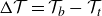 $\Delta {\mathcal{T}}= {\mathcal{T}}_b - {\mathcal{T}}_t$
is the temperature difference between the two plates, is the time scale associated with the problem. Consequently, the velocity scale used for non-dimensionalisation is
$\Delta {\mathcal{T}}= {\mathcal{T}}_b - {\mathcal{T}}_t$
is the temperature difference between the two plates, is the time scale associated with the problem. Consequently, the velocity scale used for non-dimensionalisation is
 $u_f = H/ t_f$
. The horizontal and wall-normal components of coordinates are
$u_f = H/ t_f$
. The horizontal and wall-normal components of coordinates are
 $\boldsymbol{x}=(x, z)$
, and velocity is
$\boldsymbol{x}=(x, z)$
, and velocity is
 $\boldsymbol{u} = (u, w)$
.
$\boldsymbol{u} = (u, w)$
.
The RBC is governed by the Oberbeck–Boussinesq equations (OBEs). Here,
 $\Delta {\mathcal{T}}$
is considered small so that the Boussinesq approximation is applicable. The following are the non-dimensionalised forms of the OBEs governing velocity
$\Delta {\mathcal{T}}$
is considered small so that the Boussinesq approximation is applicable. The following are the non-dimensionalised forms of the OBEs governing velocity
 $\boldsymbol{u}$
and temperature
$\boldsymbol{u}$
and temperature
 ${\mathcal{T}}$
:
${\mathcal{T}}$
:
 \begin{align} \boldsymbol{\nabla} \boldsymbol{\cdot} \boldsymbol{u} = 0, \end{align}
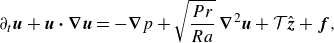 \begin{align} \partial _t{\boldsymbol{u}} + \boldsymbol{u} \boldsymbol{\cdot} \boldsymbol{\nabla} \boldsymbol{u} = -\boldsymbol{\nabla} p + \sqrt {\dfrac {Pr}{Ra}}\, \boldsymbol{\nabla} ^2\boldsymbol{u} + {\mathcal{T}} {\hat{\boldsymbol{z}}} + \boldsymbol{f}, \end{align}
 \begin{align} \partial _t{\mathcal{T}} + \boldsymbol{u} \boldsymbol{\cdot} \boldsymbol{\nabla} {\mathcal{T}} = \cfrac {1}{\sqrt {Ra\, Pr}}\,\boldsymbol{\nabla} ^2 {\mathcal{T}} + f_{\mathcal{T}}. \end{align}
In (2.2) and (2.3),
 $\boldsymbol{f}$
and
$\boldsymbol{f}$
and
 $f_{\mathcal{T}}$
are suitably chosen forcing terms. For DNS, both
$f_{\mathcal{T}}$
are suitably chosen forcing terms. For DNS, both
 $\boldsymbol{f}$
and
$\boldsymbol{f}$
and
 $f_{\mathcal{T}}$
are 0. As discussed later, in § 2.2, for the presented method, the expressions for the forcing terms
$f_{\mathcal{T}}$
are 0. As discussed later, in § 2.2, for the presented method, the expressions for the forcing terms
 $\boldsymbol{f}$
and
$\boldsymbol{f}$
and
 $f_{\mathcal{T}}$
are such that certain triad interactions are removed, suppressing the formation of convection rolls with chosen
$f_{\mathcal{T}}$
are such that certain triad interactions are removed, suppressing the formation of convection rolls with chosen
 $\Gamma _r$
.
$\Gamma _r$
.
The walls are impermeable where Dirichlet boundary conditions are applied for both
 ${\mathcal{T}}$
and
${\mathcal{T}}$
and
 $\boldsymbol{u}$
. We consider only the no-slip boundaries so that
$\boldsymbol{u}$
. We consider only the no-slip boundaries so that
 $\boldsymbol{u}=0$
. The boundary conditions for
$\boldsymbol{u}=0$
. The boundary conditions for
 ${\mathcal{T}}$
are
${\mathcal{T}}$
are
 ${\mathcal{T}}=1$
at
${\mathcal{T}}=1$
at
 $z=0$
, and
$z=0$
, and
 $\boldsymbol{u} = {\mathcal{T}} =0$
at
$\boldsymbol{u} = {\mathcal{T}} =0$
at
 $z=1$
. In the horizontal direction, a periodic boundary condition is applied for both
$z=1$
. In the horizontal direction, a periodic boundary condition is applied for both
 ${\mathcal{T}}$
and
${\mathcal{T}}$
and
 $\boldsymbol{u}$
.
$\boldsymbol{u}$
.
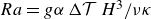
The non-dimensional parameters associated with the system are the Prandtl number
 $Pr=\nu /\kappa$
, where
$Pr=\nu /\kappa$
, where
 $\nu$
and
$\nu$
and
 $\kappa$
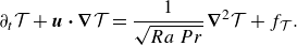
are the kinematic viscosity and thermal diffusivity, respectively, and the Rayleigh number
$\kappa$
are the kinematic viscosity and thermal diffusivity, respectively, and the Rayleigh number
 $Ra = {g\alpha\, \Delta {\mathcal{T}}\, H^3}/{\nu \kappa }$
, denoting the relative strength of thermal driving with respect to viscous dissipation. Once statistical stationarity is achieved in the simulations, the thermal energy input to the system is balanced by the viscous dissipation. Heat transport balances the thermal dissipation. Shraiman & Siggia (Reference Shraiman and Siggia1990) and Ahlers et al. (Reference Ahlers, Grossmann and Lohse2009) derived the kinetic and thermal dissipation rates from the kinetic energy and temperature variance budget equations: respectively,
$Ra = {g\alpha\, \Delta {\mathcal{T}}\, H^3}/{\nu \kappa }$
, denoting the relative strength of thermal driving with respect to viscous dissipation. Once statistical stationarity is achieved in the simulations, the thermal energy input to the system is balanced by the viscous dissipation. Heat transport balances the thermal dissipation. Shraiman & Siggia (Reference Shraiman and Siggia1990) and Ahlers et al. (Reference Ahlers, Grossmann and Lohse2009) derived the kinetic and thermal dissipation rates from the kinetic energy and temperature variance budget equations: respectively,
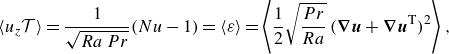 \begin{align} \langle u_z {\mathcal{T}} \rangle = \dfrac {1}{\sqrt {Ra\,Pr}}(Nu - 1) = \langle \varepsilon \rangle = \left \langle \dfrac {1}{2} \sqrt {\dfrac {Pr}{Ra}}\,(\boldsymbol{\nabla} \boldsymbol{u} + \boldsymbol{\nabla} \boldsymbol{u}^{\textrm T})^2 \right \rangle , \end{align}
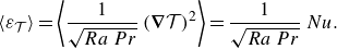 \begin{align} \langle \varepsilon _{\mathcal{T}} \rangle = \left \langle \dfrac {1}{\sqrt {Ra\,Pr}}\, (\boldsymbol{\nabla} {\mathcal{T}})^2 \right \rangle = \dfrac {1}{\sqrt {Ra\,Pr}}\,Nu. \end{align}
In these expressions,
 $\langle \cdot \rangle$
indicates time and volume averaging, and
$\langle \cdot \rangle$
indicates time and volume averaging, and
 $\varepsilon$
and
$\varepsilon$
and
 $\varepsilon _{\mathcal{T}}$
are viscous and thermal dissipation, respectively. The Nusselt number
$\varepsilon _{\mathcal{T}}$
are viscous and thermal dissipation, respectively. The Nusselt number
 $Nu$
is the dimensionless heat transport, which is an output of the system. We have also used volume averaging and time averaging, denoted by
$Nu$
is the dimensionless heat transport, which is an output of the system. We have also used volume averaging and time averaging, denoted by
 $\langle \cdot \rangle _V$
and
$\langle \cdot \rangle _V$
and
 $\langle \cdot \rangle _t$
, respectively. Specifically, for performance measures, we define the volume-averaged Reynolds number
$\langle \cdot \rangle _t$
, respectively. Specifically, for performance measures, we define the volume-averaged Reynolds number
 $\textit{Re} = \sqrt {\textit{Re}_x^2 + \textit{Re}_z^2}$
, where
$\textit{Re} = \sqrt {\textit{Re}_x^2 + \textit{Re}_z^2}$
, where
 \begin{align} & \textit{Re}_x = \sqrt {\langle u^2 \rangle _V}\,H / \nu ,\\[-8pt]\nonumber \end{align}
 \begin{align} & \textit{Re}_z = \sqrt {\langle w^2 \rangle _V}\,H / \nu . \\[6pt] \nonumber \end{align}
2.1. Numerical simulations
In this paper, we perform calculations for two
 $[Ra, Pr]$
combinations,
$[Ra, Pr]$
combinations,
 $[10^8, 10]$
and
$[10^8, 10]$
and
 $[10^9, 3]$
. The computational domain and grid resolutions of the present simulations are the same as those reported for their DNS for the chosen
$[10^9, 3]$
. The computational domain and grid resolutions of the present simulations are the same as those reported for their DNS for the chosen
 $[Ra, Pr]$
by Wang et al. (Reference Wang, Verzicco, Lohse and Shishkina2020). Therefore, all simulations presented here are fully resolved as in the DNS. Simulations are performed in a computational domain of aspect ratio
$[Ra, Pr]$
by Wang et al. (Reference Wang, Verzicco, Lohse and Shishkina2020). Therefore, all simulations presented here are fully resolved as in the DNS. Simulations are performed in a computational domain of aspect ratio
 $\Gamma = L_x/H = 8$
, with
$\Gamma = L_x/H = 8$
, with
 $H=1$
, the distance between the two plates for both
$H=1$
, the distance between the two plates for both
 $[Ra, Pr]$
combinations considered. For
$[Ra, Pr]$
combinations considered. For
 $[Ra, Pr]=[10^8, 10]$
,
$[Ra, Pr]=[10^8, 10]$
,
 $2048\times 256$
grid points are used in the horizontal and vertical directions, respectively, and
$2048\times 256$
grid points are used in the horizontal and vertical directions, respectively, and
 $4096\times 512$
grid points resolve the computational domain for
$4096\times 512$
grid points resolve the computational domain for
 $[Ra, Pr]=[10^9, 3]$
. As suggested by Wang et al. (Reference Wang, Verzicco, Lohse and Shishkina2020), the fastest way to capture the multiple states in DNS is to prescribe the convection rolls with the target aspect ratio in the initial conditions. If
$[Ra, Pr]=[10^9, 3]$
. As suggested by Wang et al. (Reference Wang, Verzicco, Lohse and Shishkina2020), the fastest way to capture the multiple states in DNS is to prescribe the convection rolls with the target aspect ratio in the initial conditions. If
 $n^{(i)}$
is the number of rolls in the initial state, then the prescribed initial velocity and temperature fields are
$n^{(i)}$
is the number of rolls in the initial state, then the prescribed initial velocity and temperature fields are
 \begin{eqnarray} & \boldsymbol{u}= [u(x,z), w(x,z)] =\left [ \sin \left (\dfrac {n^{(i)} \unicode{x03C0} x}{\Gamma }\right )\cos \left (\unicode{x03C0} z\right ),-\cos \left (\dfrac {n^{(i)} \unicode{x03C0} x}{\Gamma }\right )\sin \left (\unicode{x03C0} z\right ) \right ], \end{eqnarray}
 \begin{eqnarray} & {\mathcal{T}} = 1-z. \end{eqnarray}
The OBEs in (2.1)–(2.3) were solved using the pseudo-spectral code based on the Dedalus partial differential equation solving framework (Burns et al. Reference Burns, Vasil, Oishi, Lecoanet and Brown2020). For spatial discretisation, Fourier and Chebychev expansions were used in the
 $x$
and
$x$
and
 $z$
directions. For dealiasing, we utilise the ‘
$z$
directions. For dealiasing, we utilise the ‘
 $3/2$
’ rule. Time integration was performed by the third-order four-stage combination of a diagonally implicit Runge–Kutta scheme and an explicit Runge–Kutta scheme (RK443 time stepper). Time snapshots were stored at a time interval of one free-fall time unit for a period of 500 free-fall time units for the proposed forcing methodology switching on the forcing terms in (2.2) and (2.3); this time frame was sufficient for yielding the multiple states. However, DNS for
$3/2$
’ rule. Time integration was performed by the third-order four-stage combination of a diagonally implicit Runge–Kutta scheme and an explicit Runge–Kutta scheme (RK443 time stepper). Time snapshots were stored at a time interval of one free-fall time unit for a period of 500 free-fall time units for the proposed forcing methodology switching on the forcing terms in (2.2) and (2.3); this time frame was sufficient for yielding the multiple states. However, DNS for
 $[Ra, Pr]=[10^9, 3]$
initiated with the target roll states (2.8) and (2.9) did not converge to a statistically stationary state within that interval, and therefore had to be run longer.
$[Ra, Pr]=[10^9, 3]$
initiated with the target roll states (2.8) and (2.9) did not converge to a statistically stationary state within that interval, and therefore had to be run longer.
2.2. Definitions of
 $\boldsymbol{f}$
and
$f_{\mathcal{T}}$
: scale-to-scale energy transfer
$\boldsymbol{f}$
and
$f_{\mathcal{T}}$
: scale-to-scale energy transfer


The forcing terms in (2.2) and (2.3) remain to be defined. These terms are defined based on the observation that the characteristic horizontal wavenumber associated with the mean horizontal size of the convection rolls (
 $k_r$
, say) acts as the mediator in wavenumber triads involved in establishing essential energy cascade processes at a statistical stationary state. To elaborate on this point, we quantify the nonlinear interactions in OBEs in (2.1)–(2.3).
$k_r$
, say) acts as the mediator in wavenumber triads involved in establishing essential energy cascade processes at a statistical stationary state. To elaborate on this point, we quantify the nonlinear interactions in OBEs in (2.1)–(2.3).
To quantify the scale-to-scale energy transfers among the streamwise wavenumbers due to nonlinear triadic scale interactions, first Fourier transforms are performed for the temperature and components of the velocity fields. Then, corresponding to each wavenumber
 $l ({2\unicode{x03C0} }/{L_x})$
(where
$l ({2\unicode{x03C0} }/{L_x})$
(where
 $l$
is the integer wavenumber) or physical length scale
$l$
is the integer wavenumber) or physical length scale
 $L_x/l$
, the inverse transform is performed, thus obtaining the following flow fields corresponding to each physical length scale in the physical space:
$L_x/l$
, the inverse transform is performed, thus obtaining the following flow fields corresponding to each physical length scale in the physical space:
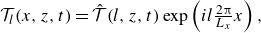 \begin{eqnarray} & {\mathcal{T}}_l(x, z, t) = \hat {\mathcal{T}}(l, z, t)\exp\left({il \frac {2\unicode{x03C0} }{L_x}x}\right), \end{eqnarray}
 \begin{eqnarray} & \boldsymbol{u}_l(x, z, t) = \hat {\boldsymbol{u}}(l, z, t)\exp\left({il \frac {2\unicode{x03C0} }{L_x}x}\right). \end{eqnarray}
Now let us assume a triad
 $[k, p, m] ({2\unicode{x03C0} }/{L_x})$
, where,
$[k, p, m] ({2\unicode{x03C0} }/{L_x})$
, where,
 $k$
,
$k$
,
 $p$
and
$p$
and
 $m=k-p$
are the integer receiver, donator and mediator streamwise wavenumbers, respectively. In the rest of the paper, the aforementioned convention is used to express the wavenumbers involved in a triad. Favier, Silvers & Proctor (Reference Favier, Silvers and Proctor2014) defined the transfer functions quantifying the scale-to-scale energy transfer between donator
$m=k-p$
are the integer receiver, donator and mediator streamwise wavenumbers, respectively. In the rest of the paper, the aforementioned convention is used to express the wavenumbers involved in a triad. Favier, Silvers & Proctor (Reference Favier, Silvers and Proctor2014) defined the transfer functions quantifying the scale-to-scale energy transfer between donator
 $p$
and receiver
$p$
and receiver
 $k$
, mediated by the mediator
$k$
, mediated by the mediator
 $m=k-p$
. The expressions for
$m=k-p$
. The expressions for
 $T_{\mathcal{T}}(k, p)$
, quantifying the scale-to-scale temperature variance transfer, and
$T_{\mathcal{T}}(k, p)$
, quantifying the scale-to-scale temperature variance transfer, and
 $T(k, p)$
, quantifying the scale-to-scale kinetic energy transfer, are
$T(k, p)$
, quantifying the scale-to-scale kinetic energy transfer, are
 \begin{align} T_{\mathcal{T}}(k, p) &= -\int _V {\mathcal{T}}_k (\boldsymbol{u}_{k-p} \boldsymbol{\cdot} \boldsymbol{\nabla} {\mathcal{T}}_p )\, {\textrm d}V ,\\[-10pt]\nonumber \end{align}
 \begin{align} T(k, p) & = -\int _V \boldsymbol{u}_k \boldsymbol{\cdot} (\boldsymbol{u}_{k-p} \boldsymbol{\cdot} \boldsymbol{\nabla} \boldsymbol{u}_p )\, {\textrm d}V. \\[6pt] \nonumber \end{align}
The integrands in the right-hand sides of (2.12) and (2.13) arise from the nonlinear advection terms of the OBEs, and are essentially the transport terms in the temperature variance and kinetic energy budget equations, respectively. For
 $T_{\mathcal{T}}(k, p) \gt 0$
(
$T_{\mathcal{T}}(k, p) \gt 0$
(
 $T(k, p) \gt 0$
), a positive amount of temperature variance (kinetic energy) is transferred from the donator wavenumber
$T(k, p) \gt 0$
), a positive amount of temperature variance (kinetic energy) is transferred from the donator wavenumber
 $p$
to the receiver wavenumber
$p$
to the receiver wavenumber
 $k$
. Consequently, due to the principles of transactions, the transfer functions are anti-symmetric with respect to
$k$
. Consequently, due to the principles of transactions, the transfer functions are anti-symmetric with respect to
 $k=p$
, i.e.
$k=p$
, i.e.
 $T_{\mathcal{T}}(k, p)=-T_{\mathcal{T}}(p, k)$
and
$T_{\mathcal{T}}(k, p)=-T_{\mathcal{T}}(p, k)$
and
 $T(k, p) = -T(p, k)$
. The mediator wavenumber
$T(k, p) = -T(p, k)$
. The mediator wavenumber
 $k-p$
mediates the energy transfer process (Verma Reference Verma2019; Bose, Kannan & Zhu Reference Bose, Kannan and Zhu2024).
$k-p$
mediates the energy transfer process (Verma Reference Verma2019; Bose, Kannan & Zhu Reference Bose, Kannan and Zhu2024).
Bose et al. (Reference Bose, Kannan and Zhu2024) used the above expressions for scale-to-scale energy transfer functions (2.12) and (2.13) to study the dominant energy transfer processes in 2-D RBC. Their flow was for
 $[Ra, Pr]=[10^8, 10]$
; of the multiple states, only the
$[Ra, Pr]=[10^8, 10]$
; of the multiple states, only the
 $\Gamma _r=1$
state (here,
$\Gamma _r=1$
state (here,
 $\Gamma _r=\Gamma /n=1$
, where
$\Gamma _r=\Gamma /n=1$
, where
 $n$
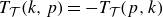
is the number of rolls in the converged state) was considered. Based on their DNS data, they showed that kinetic energy and temperature variance transfers between scales in a statistically stationary state are dominated by: (i) the energy transfer to/from the convection rolls, and (ii) the scale-to-scale kinetic energy and temperature variance cascades mediated by the convection rolls. These energy transfer processes are depicted here by plotting
$n$
is the number of rolls in the converged state) was considered. Based on their DNS data, they showed that kinetic energy and temperature variance transfers between scales in a statistically stationary state are dominated by: (i) the energy transfer to/from the convection rolls, and (ii) the scale-to-scale kinetic energy and temperature variance cascades mediated by the convection rolls. These energy transfer processes are depicted here by plotting
 $T_{\mathcal{T}}(k, p)$
in figure 1, and
$T_{\mathcal{T}}(k, p)$
in figure 1, and
 $T(k, p)$
in figure 2, for the statistically stationary multiple states for
$T(k, p)$
in figure 2, for the statistically stationary multiple states for
 $[Ra, Pr]=[10^8, 10]$
. For this
$[Ra, Pr]=[10^8, 10]$
. For this
 $[Ra, Pr]$
combination, Wang et al. (Reference Wang, Verzicco, Lohse and Shishkina2020) found only two states – either
$[Ra, Pr]$
combination, Wang et al. (Reference Wang, Verzicco, Lohse and Shishkina2020) found only two states – either
 $n=6$
or
$n=6$
or
 $n=8$
convection rolls were obtained, with mean aspect ratios
$n=8$
convection rolls were obtained, with mean aspect ratios
 $\Gamma _r=4/3$
and 1, respectively.
$\Gamma _r=4/3$
and 1, respectively.
Figure 1. Scale-to-scale temperature variance transfer function
 $T_{\mathcal{T}}(k, p)$
from DNS of 2-D RBC at
$T_{\mathcal{T}}(k, p)$
from DNS of 2-D RBC at
 $[Ra, Pr]=[10^8, 10]$
: (
$[Ra, Pr]=[10^8, 10]$
: (
 $a$
)
$a$
)
 $n=6$
state (
$n=6$
state (
 $\Gamma _r=4/3$
), (
$\Gamma _r=4/3$
), (
 $b$
)
$b$
)
 $n=8$
state (
$n=8$
state (
 $\Gamma _r=1$
) (Bose et al. Reference Bose, Kannan and Zhu2024). Here,
$\Gamma _r=1$
) (Bose et al. Reference Bose, Kannan and Zhu2024). Here,
 $k$
and
$k$
and
 $p$
are the receiver and donator integer horizontal wavenumbers, respectively.
$p$
are the receiver and donator integer horizontal wavenumbers, respectively.
For
 $T_{\mathcal{T}}(k, p)$
, the scale-to-scale forward temperature variance cascade is the only dominant process (marked by arrows) for both cases in figure 1. This represents a forward cascade because
$T_{\mathcal{T}}(k, p)$
, the scale-to-scale forward temperature variance cascade is the only dominant process (marked by arrows) for both cases in figure 1. This represents a forward cascade because
 $T_{\mathcal{T}}(k, p)\gt 0$
for
$T_{\mathcal{T}}(k, p)\gt 0$
for
 $k\gt p$
(the red patch), and the corresponding blue patch, where
$k\gt p$
(the red patch), and the corresponding blue patch, where
 $T_{\mathcal{T}}(k, p) \lt 0$
, corresponds to
$T_{\mathcal{T}}(k, p) \lt 0$
, corresponds to
 $p \gt k$
: energy is transferred from larger scales to smaller scales. These two patches are positioned at a constant distance away from the line
$p \gt k$
: energy is transferred from larger scales to smaller scales. These two patches are positioned at a constant distance away from the line
 $k=p$
(the apparent curvature is due to the abscissa and the ordinate being plotted on logarithmic scale). Obviously, the separation is equal to the mediator wavenumber
$k=p$
(the apparent curvature is due to the abscissa and the ordinate being plotted on logarithmic scale). Obviously, the separation is equal to the mediator wavenumber
 $m$
, and the diagrams indicate it to be a constant. In fact,
$m$
, and the diagrams indicate it to be a constant. In fact,
 $m=k-p=\pm k_r$
, where
$m=k-p=\pm k_r$
, where
 $k_r$
is the characteristic integer wavenumber corresponding to the mean horizontal wavelength of the rolls,
$k_r$
is the characteristic integer wavenumber corresponding to the mean horizontal wavelength of the rolls,
 $\lambda _r$
. For
$\lambda _r$
. For
 $n=6$
and 8 states,
$n=6$
and 8 states,
 $\lambda _r={8}/{3}$
and
$\lambda _r={8}/{3}$
and
 ${8}/{4}$
, respectively, so that,
${8}/{4}$
, respectively, so that,
 $k_r=3$
and 4 (as
$k_r=3$
and 4 (as
 $k_r= {L_x}/{\lambda _r}$
), respectively. Therefore, the triads involved in the process are of the form
$k_r= {L_x}/{\lambda _r}$
), respectively. Therefore, the triads involved in the process are of the form
 $[k, p, m = k-p = \pm k_r] ({2\unicode{x03C0} }/{L_x})$
. Clearly, the cascade process mediated by the rolls is essential for the sustenance of the statistically stationary state for both cases. Physically, the forward cascade is a consequence of an instability of the base flow comprising the convection rolls with characteristic wavenumber
$[k, p, m = k-p = \pm k_r] ({2\unicode{x03C0} }/{L_x})$
. Clearly, the cascade process mediated by the rolls is essential for the sustenance of the statistically stationary state for both cases. Physically, the forward cascade is a consequence of an instability of the base flow comprising the convection rolls with characteristic wavenumber
 $k_r$
.
$k_r$
.
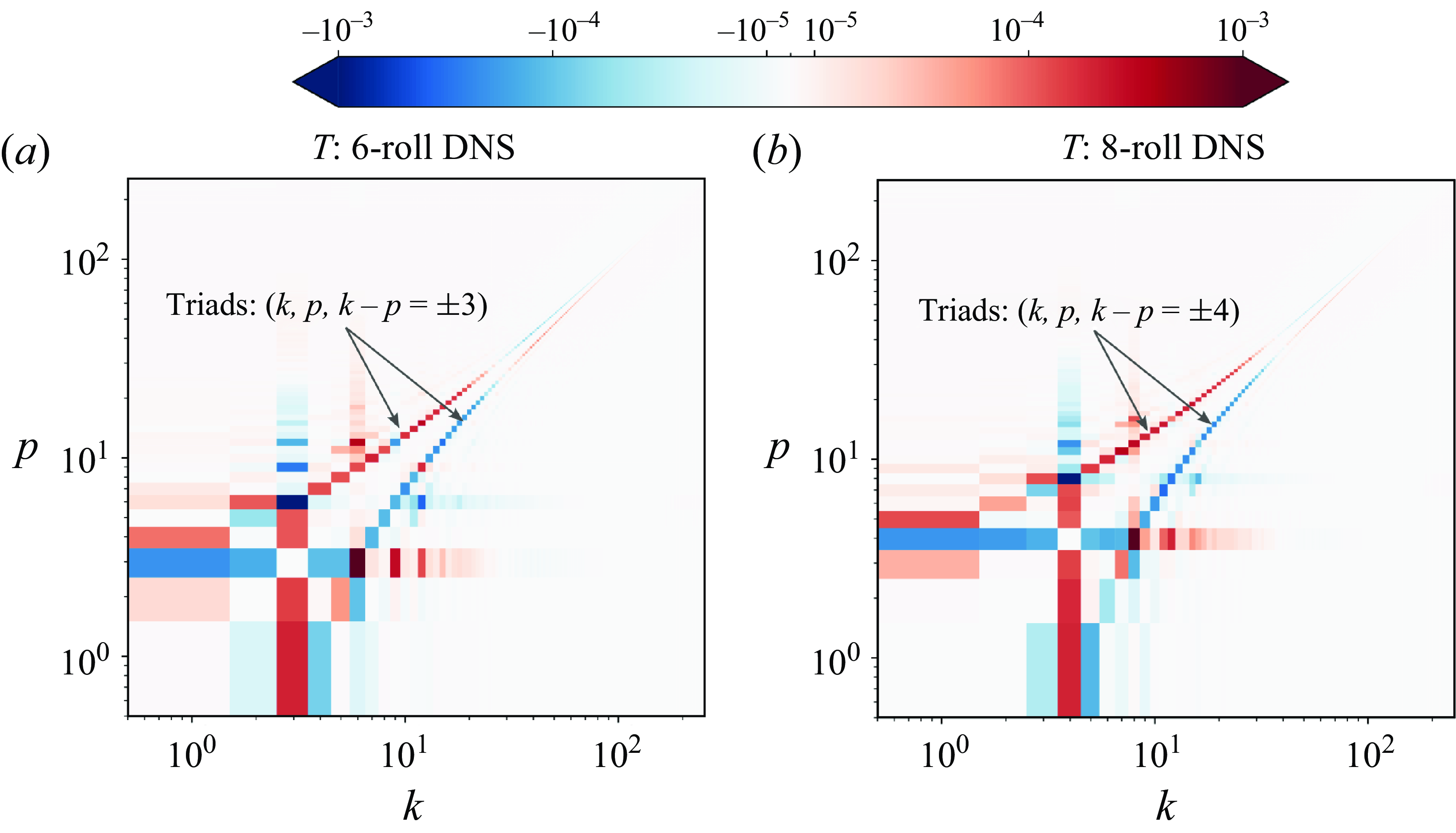
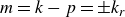
Figure 2. Scale-to-scale kinetic energy transfer function
 $T(k, p)$
from DNS of 2-D RBC at
$T(k, p)$
from DNS of 2-D RBC at
 $[Ra, Pr]=[10^8, 10]$
: (
$[Ra, Pr]=[10^8, 10]$
: (
 $a$
)
$a$
)
 $n=6$
state (
$n=6$
state (
 $\Gamma _r=4/3$
), (
$\Gamma _r=4/3$
), (
 $b$
)
$b$
)
 $n=8$
state (
$n=8$
state (
 $\Gamma _r=1$
) (Bose et al. Reference Bose, Kannan and Zhu2024). Here,
$\Gamma _r=1$
) (Bose et al. Reference Bose, Kannan and Zhu2024). Here,
 $k$
and
$k$
and
 $p$
are the receiver and donator integer horizontal wavenumbers, respectively.
$p$
are the receiver and donator integer horizontal wavenumbers, respectively.
In addition to the energy cascade process (marked by arrows), the energy transfers to/from the convection rolls are also relevant for scale-to-scale kinetic energy transfer process in figure 2 for both states. The cascade process is inverse in nature, i.e.
 $T(k, p)\lt 0$
for
$T(k, p)\lt 0$
for
 $k\gt p$
(the blue patch); energy transfer is from small scales to larger scales. As is for the temperature variance cascades in figure 1, the involved triads are of the form
$k\gt p$
(the blue patch); energy transfer is from small scales to larger scales. As is for the temperature variance cascades in figure 1, the involved triads are of the form
 $[k, p, k-p= \pm k_r]({2\unicode{x03C0} }/{L_x})$
. From these two figures, it becomes evident that the scale-to-scale energy cascades mediated by the convection rolls are crucial for their sustenance.
$[k, p, k-p= \pm k_r]({2\unicode{x03C0} }/{L_x})$
. From these two figures, it becomes evident that the scale-to-scale energy cascades mediated by the convection rolls are crucial for their sustenance.
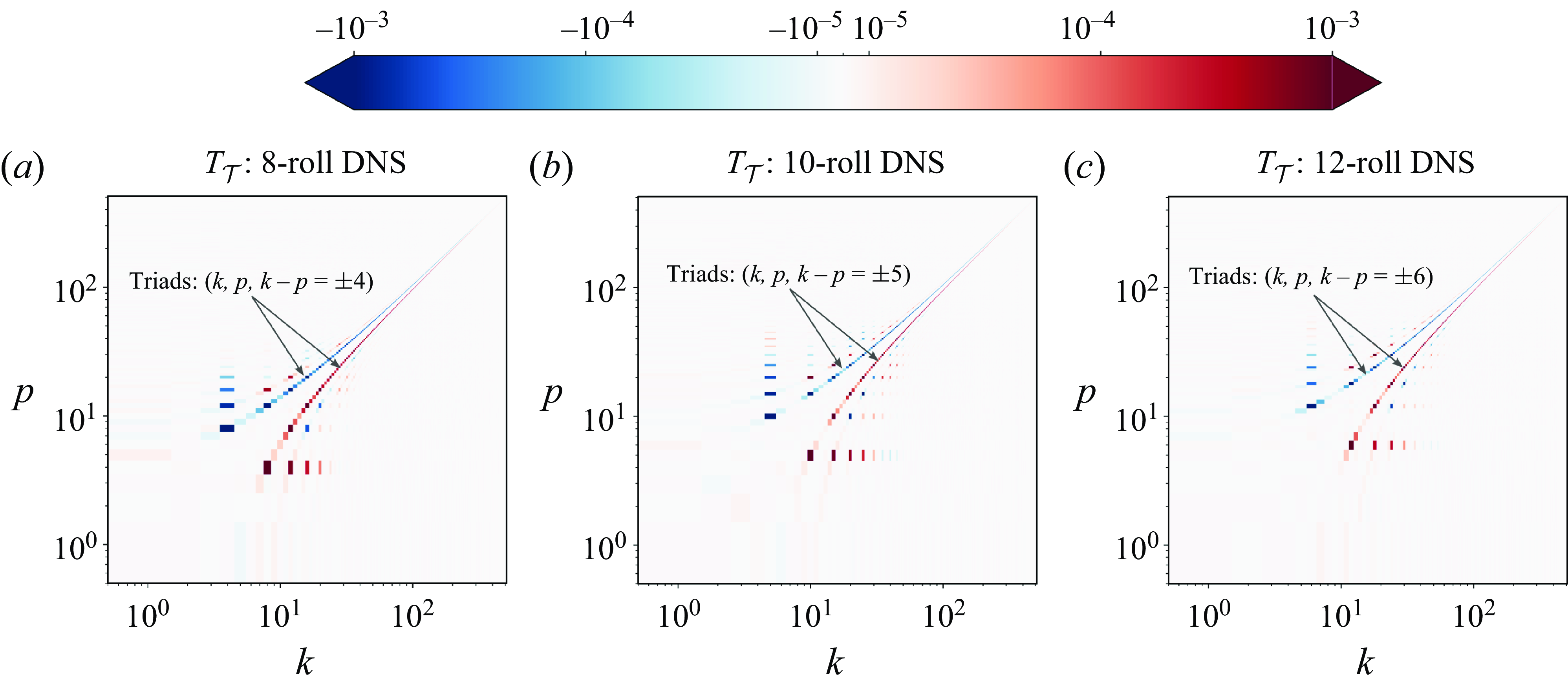
Figure 3. Scale-to-scale temperature variance transfer function
 $T_{\mathcal{T}}(k, p)$
from DNS of 2-D RBC at
$T_{\mathcal{T}}(k, p)$
from DNS of 2-D RBC at
 $[Ra, Pr]=[10^9, 3]$
: (
$[Ra, Pr]=[10^9, 3]$
: (
 $a$
)
$a$
)
 $n=8$
state (
$n=8$
state (
 $\Gamma _r=1$
), (
$\Gamma _r=1$
), (
 $b$
)
$b$
)
 $n=10$
state (
$n=10$
state (
 $\Gamma _r=4/5$
), (c)
$\Gamma _r=4/5$
), (c)
 $n=12$
state (
$n=12$
state (
 $\Gamma _r=2/3$
). Here,
$\Gamma _r=2/3$
). Here,
 $k$
and
$k$
and
 $p$
are the receiver and donator integer horizontal wavenumbers, respectively.
$p$
are the receiver and donator integer horizontal wavenumbers, respectively.
Similar analyses performed for the multiple states obtained for
 $[Ra, Pr]=[10^9, 3]$
also reveal that the convection rolls mediate energy in cascade processes. Wang et al. (Reference Wang, Verzicco, Lohse and Shishkina2020) reported the existence of three states:
$[Ra, Pr]=[10^9, 3]$
also reveal that the convection rolls mediate energy in cascade processes. Wang et al. (Reference Wang, Verzicco, Lohse and Shishkina2020) reported the existence of three states:
 $n=8$
(
$n=8$
(
 $\Gamma _r=1$
),
$\Gamma _r=1$
),
 $n=10$
(
$n=10$
(
 $\Gamma _r=4/5$
) and
$\Gamma _r=4/5$
) and
 $n=12$
(
$n=12$
(
 $\Gamma _r=2/3$
) convection rolls were obtained in a computational domain with aspect ratio
$\Gamma _r=2/3$
) convection rolls were obtained in a computational domain with aspect ratio
 $\Gamma =8$
. The temperature variance transfer function
$\Gamma =8$
. The temperature variance transfer function
 $T_{\mathcal{T}}(k, p)$
and kinetic energy transfer function
$T_{\mathcal{T}}(k, p)$
and kinetic energy transfer function
 $T(k, p)$
from DNS capturing these roll states are shown in figures 3 and 4, respectively. For
$T(k, p)$
from DNS capturing these roll states are shown in figures 3 and 4, respectively. For
 $T_{\mathcal{T}}(k, p)$
, for all three cases, cascade mediated by rolls is the only dominant process. In addition to the cascade process, for
$T_{\mathcal{T}}(k, p)$
, for all three cases, cascade mediated by rolls is the only dominant process. In addition to the cascade process, for
 $T(k, p)$
, as for
$T(k, p)$
, as for
 $[Ra, Pr]=[10^8, 10]$
, the energy transfer to/from the convection rolls is also relevant.
$[Ra, Pr]=[10^8, 10]$
, the energy transfer to/from the convection rolls is also relevant.
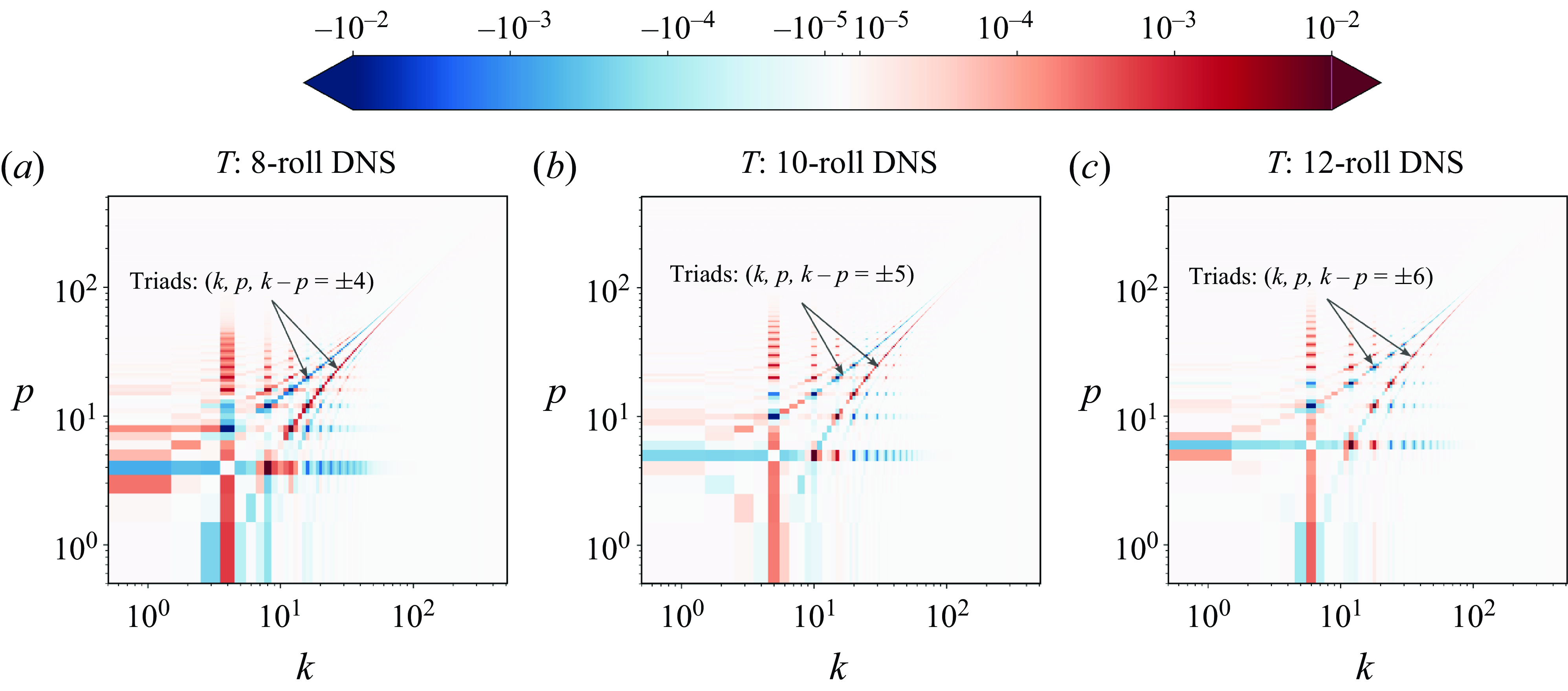
Figure 4. Scale-to-scale kinetic energy transfer function
 $T(k, p)$
from DNS of 2-D RBC at
$T(k, p)$
from DNS of 2-D RBC at
 $[Ra, Pr]=[10^9, 3]$
: (
$[Ra, Pr]=[10^9, 3]$
: (
 $a$
)
$a$
)
 $n=8$
state (
$n=8$
state (
 $\Gamma _r=1$
), (
$\Gamma _r=1$
), (
 $b$
)
$b$
)
 $n=10$
state (
$n=10$
state (
 $\Gamma _r=4/5$
), (c)
$\Gamma _r=4/5$
), (c)
 $n=12$
state (
$n=12$
state (
 $\Gamma _r=2/3$
). Here,
$\Gamma _r=2/3$
). Here,
 $k$
and
$k$
and
 $p$
are the receiver and donator integer horizontal wavenumbers, respectively.
$p$
are the receiver and donator integer horizontal wavenumbers, respectively.
So in order to suppress the emergence of convection rolls of a particular value or range of
 $\Gamma _r$
, the triad interactions involving as the mediator the target characteristic wavenumber(s) for roll formation (
$\Gamma _r$
, the triad interactions involving as the mediator the target characteristic wavenumber(s) for roll formation (
 $k_t = [k_1, k_2, \ldots ]$
, say) must be removed. The forcing terms
$k_t = [k_1, k_2, \ldots ]$
, say) must be removed. The forcing terms
 $\boldsymbol{f}$
in (2.2) and
$\boldsymbol{f}$
in (2.2) and
 $f_{\mathcal{T}}$
in (2.3) are used to remove such triad interactions. Verma (Reference Verma2019) described the function of the mediator wavenumber (see chapter 4 and figure 4.3 therein, and also § 5.4.3 in Schmid, Henningson & Jankowski Reference Schmid, Henningson and Jankowski2002). The role of the velocity field due to the mediator wavenumber
$f_{\mathcal{T}}$
in (2.3) are used to remove such triad interactions. Verma (Reference Verma2019) described the function of the mediator wavenumber (see chapter 4 and figure 4.3 therein, and also § 5.4.3 in Schmid, Henningson & Jankowski Reference Schmid, Henningson and Jankowski2002). The role of the velocity field due to the mediator wavenumber
 $m=k-p$
in (2.12) and (2.13), for example, is to advect the temperature/velocity field due to the donor wavenumber
$m=k-p$
in (2.12) and (2.13), for example, is to advect the temperature/velocity field due to the donor wavenumber
 $p$
as it exchanges energy with the temperature/velocity field due to the receiver wavenumber
$p$
as it exchanges energy with the temperature/velocity field due to the receiver wavenumber
 $k$
. The mediator wavenumber does not receive any energy in the process, and is hence named the mediator. Because of the reality condition of the velocity field, the velocity field due to the mediator wavenumbers
$k$
. The mediator wavenumber does not receive any energy in the process, and is hence named the mediator. Because of the reality condition of the velocity field, the velocity field due to the mediator wavenumbers
 $m=\pm k_r$
is
$m=\pm k_r$
is
 $\boldsymbol{u}_{k_r}$
(see (2.11)). Therefore, based on the above discussions and the expressions for the transfer functions in (2.12) and (2.13), to drop all triad interactions mediated by wavenumbers
$\boldsymbol{u}_{k_r}$
(see (2.11)). Therefore, based on the above discussions and the expressions for the transfer functions in (2.12) and (2.13), to drop all triad interactions mediated by wavenumbers
 $k_t$
, the forcing terms are defined as
$k_t$
, the forcing terms are defined as
 \begin{eqnarray}& f_{\mathcal{T}} = {\sum }_{k_t}\boldsymbol{u}_{k_t} \boldsymbol{\cdot} \boldsymbol{\nabla} {\mathcal{T}}, \end{eqnarray}
 \begin{eqnarray} & \boldsymbol{f} = {\sum }_{k_t} \boldsymbol{u}_{k_t} \boldsymbol{\cdot} \boldsymbol{\nabla} \boldsymbol{u}. \end{eqnarray}
The effect of the forcing terms on the OBEs in (2.1)–(2.3) may be understood by noting the overall nonlinear terms of the proposed forcing methodology,
 $(\boldsymbol{u}-\sum _{k_t}\boldsymbol{u}_{k_t})\boldsymbol{\cdot} \boldsymbol{\nabla} \boldsymbol{u}$
and
$(\boldsymbol{u}-\sum _{k_t}\boldsymbol{u}_{k_t})\boldsymbol{\cdot} \boldsymbol{\nabla} \boldsymbol{u}$
and
 $(\boldsymbol{u}-\sum _{k_t}\boldsymbol{u}_{k_t})\boldsymbol{\cdot} \boldsymbol{\nabla} {\mathcal{T}}$
, in the momentum and temperature equations, respectively. As in linear/weakly nonlinear analysis, following Reynolds decomposition
$(\boldsymbol{u}-\sum _{k_t}\boldsymbol{u}_{k_t})\boldsymbol{\cdot} \boldsymbol{\nabla} {\mathcal{T}}$
, in the momentum and temperature equations, respectively. As in linear/weakly nonlinear analysis, following Reynolds decomposition
 $\boldsymbol{u}=\boldsymbol{U}_b + \boldsymbol{u}'$
(with
$\boldsymbol{u}=\boldsymbol{U}_b + \boldsymbol{u}'$
(with
 $\boldsymbol{U}_b=0$
for the 2-D RBC system) and
$\boldsymbol{U}_b=0$
for the 2-D RBC system) and
 ${\mathcal{T}}={\mathcal{T}}_b + {\mathcal{T}}'$
, the nonlinear terms in the OBEs become
${\mathcal{T}}={\mathcal{T}}_b + {\mathcal{T}}'$
, the nonlinear terms in the OBEs become
 \begin{eqnarray} & \left(\boldsymbol{u}-{\sum }_{k_t}{\boldsymbol{u}}_{k_t}\right)\boldsymbol{\cdot} \boldsymbol{\nabla} \boldsymbol{u} =\left(\boldsymbol{u}'-{\sum }_{k_t}\boldsymbol{u}_{k_t}\right)\boldsymbol{\cdot} \boldsymbol{\nabla} \boldsymbol{u}', \end{eqnarray}
 \begin{eqnarray} & \left(\boldsymbol{u}-{\sum }_{k_t}\boldsymbol{u}_{k_t}\right)\boldsymbol{\cdot} \boldsymbol{\nabla} {\mathcal{T}} = \big(\boldsymbol{u}'-{\sum}_{k_t}\boldsymbol{u}_{k_t} \big) \boldsymbol{\cdot} \boldsymbol{\nabla} ({\mathcal{T}}_b + {\mathcal{T}}'). \end{eqnarray}
In the above expressions,
 $\sum _{k_t}\boldsymbol{u}_{k_t}$
is the component of the perturbation velocity field, with
$\sum _{k_t}\boldsymbol{u}_{k_t}$
is the component of the perturbation velocity field, with
 $\boldsymbol{u}'$
corresponding to the chosen forcing wavenumbers
$\boldsymbol{u}'$
corresponding to the chosen forcing wavenumbers
 $k_t$
. Except for the forcing terms, the nonlinear terms in the perturbation equations are the same as those without forcing. Hence the forcing should in effect eliminate the linear/weakly nonlinear growth at the forcing wavenumbers
$k_t$
. Except for the forcing terms, the nonlinear terms in the perturbation equations are the same as those without forcing. Hence the forcing should in effect eliminate the linear/weakly nonlinear growth at the forcing wavenumbers
 $k_t$
.
$k_t$
.
In the next section, we demonstrate that the removal of triad interactions mediated by one/multiple candidate wavenumbers by switching on
 $\boldsymbol{f}$
and
$\boldsymbol{f}$
and
 $f_{\mathcal{T}}$
in (2.2) and (2.3) results in the emergence of convection rolls at another unforced candidate wavenumber. If all stable states are suppressed, then this forcing methodology tends to converge to flow fields with arbitrary patterns, making it a suitable method for discovering the multiple states in 2-D RBC. Additionally, the flow statistics converge much more quickly using the proposed forcing than in DNS initiated with a target roll state as in (2.8). Furthermore, using the proposed technique, the dependence of the emergence of the multiple states on the initial conditions can be bypassed for 2-D RBC.
$f_{\mathcal{T}}$
in (2.2) and (2.3) results in the emergence of convection rolls at another unforced candidate wavenumber. If all stable states are suppressed, then this forcing methodology tends to converge to flow fields with arbitrary patterns, making it a suitable method for discovering the multiple states in 2-D RBC. Additionally, the flow statistics converge much more quickly using the proposed forcing than in DNS initiated with a target roll state as in (2.8). Furthermore, using the proposed technique, the dependence of the emergence of the multiple states on the initial conditions can be bypassed for 2-D RBC.
3. Test cases
In the following, the initial conditions for the forced simulations are a
 ${\mathcal{T}}$
field consisting of random perturbations superimposed on the linear conductive profile, and
${\mathcal{T}}$
field consisting of random perturbations superimposed on the linear conductive profile, and
 $\boldsymbol{u} = 0$
. We call this initial condition ‘random’. The DNS are initialised either with the conditions specified in (2.8) and (2.9) (we avoid cases with
$\boldsymbol{u} = 0$
. We call this initial condition ‘random’. The DNS are initialised either with the conditions specified in (2.8) and (2.9) (we avoid cases with
 $n^{(i)} \neq n$
, including state transitions that take longer simulation times), or from states obtained in the forced simulations switching off the forcing.
$n^{(i)} \neq n$
, including state transitions that take longer simulation times), or from states obtained in the forced simulations switching off the forcing.
Also in the following discussion, as obtaining accurate statistics for the roll states is not the purpose of this study, we calculate the statistics only when possible. So by the term ‘convergence’, we mean either the rate at which some statistical quantity (
 $Re$
, for example) approaches stationarity, or obtaining the desired roll state as flow structures in a simulation that has not necessarily reached statistical stationarity.
$Re$
, for example) approaches stationarity, or obtaining the desired roll state as flow structures in a simulation that has not necessarily reached statistical stationarity.
3.1. Multiple states for
$[Ra, Pr]=[10^{8}, 10]$

For
 $[Ra, Pr]=[10^{8}, 10]$
, Wang et al. (Reference Wang, Verzicco, Lohse and Shishkina2020) found two statistically stationary states:
$[Ra, Pr]=[10^{8}, 10]$
, Wang et al. (Reference Wang, Verzicco, Lohse and Shishkina2020) found two statistically stationary states:
 $n=6$
and
$n=6$
and
 $n=8$
convection rolls in a domain with
$n=8$
convection rolls in a domain with
 $\Gamma =8$
(mean aspect ratio of the rolls,
$\Gamma =8$
(mean aspect ratio of the rolls,
 $\Gamma _r=\Gamma /n=4/3$
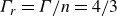
and 1, respectively). The results yielding the multiple states for this combination of control parameters are shown in figures 5 and 6.
$\Gamma _r=\Gamma /n=4/3$
and 1, respectively). The results yielding the multiple states for this combination of control parameters are shown in figures 5 and 6.
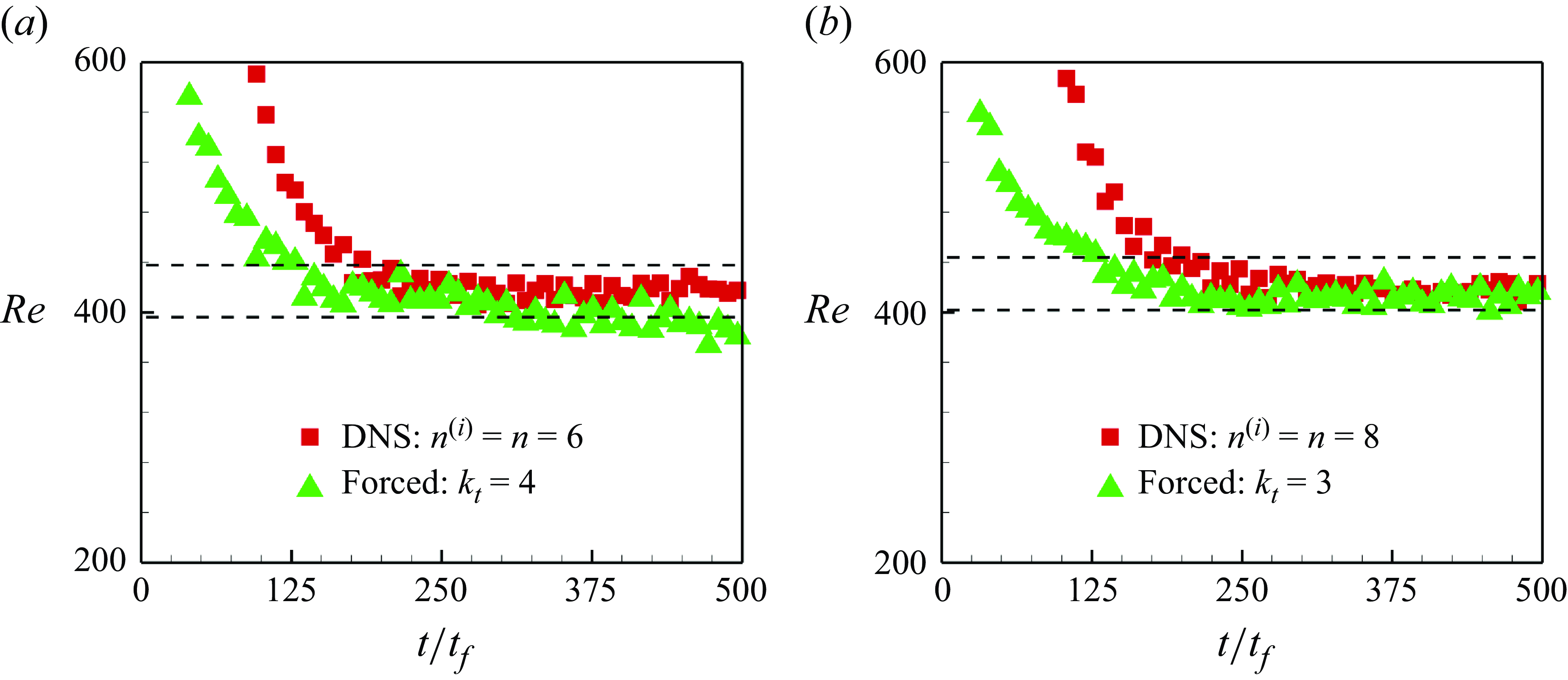
Figure 5. Plots of
 $\textit{Re}$
as a function of simulation time (
$\textit{Re}$
as a function of simulation time (
 $t/t_f$
) from direct and forced simulations for
$t/t_f$
) from direct and forced simulations for
 $[Ra, Pr]=[10^8, 10]$
: (
$[Ra, Pr]=[10^8, 10]$
: (
 $a$
) DNS initiated with
$a$
) DNS initiated with
 $n^{(i)}=n=6$
, and a forced simulation with
$n^{(i)}=n=6$
, and a forced simulation with
 $k_t=4$
; (
$k_t=4$
; (
 $b$
) DNS initiated with
$b$
) DNS initiated with
 $n^{(i)}=n=8$
, and a forced simulation with
$n^{(i)}=n=8$
, and a forced simulation with
 $k_t=3$
. The horizontal dashed lines correspond to
$k_t=3$
. The horizontal dashed lines correspond to
 $\pm 5\,\%$
of the
$\pm 5\,\%$
of the
 $\textit{Re}$
values reported by Wang et al. (Reference Wang, Verzicco, Lohse and Shishkina2020) from their DNS.
$\textit{Re}$
values reported by Wang et al. (Reference Wang, Verzicco, Lohse and Shishkina2020) from their DNS.
Figures 5(
 $a$
), 6(
$a$
), 6(
 $a$
) and 6(
$a$
) and 6(
 $b$
) show the results from DNS initialised with
$b$
) show the results from DNS initialised with
 $n^{(i)}=6$
(
$n^{(i)}=6$
(
 $\Gamma _r=4/3$
), and a forced simulation with
$\Gamma _r=4/3$
), and a forced simulation with
 $k_t=4$
(to suppress the emergence of the
$k_t=4$
(to suppress the emergence of the
 $n=8$
state with
$n=8$
state with
 $k_r=4$
and
$k_r=4$
and
 $\Gamma _r=1$
). Figure 5(
$\Gamma _r=1$
). Figure 5(
 $a$
) shows the convergence of
$a$
) shows the convergence of
 $\textit{Re}$
for the two cases with simulation time
$\textit{Re}$
for the two cases with simulation time
 $t/t_f$
. Here,
$t/t_f$
. Here,
 $\textit{Re}$
is used as the metric for comparison instead of
$\textit{Re}$
is used as the metric for comparison instead of
 $Nu$
because of its slower convergence rate. The two simulations seem to converge at similar rates;
$Nu$
because of its slower convergence rate. The two simulations seem to converge at similar rates;
 $\textit{Re}$
computed for the two simulations converges to similar values. Figures 6(
$\textit{Re}$
computed for the two simulations converges to similar values. Figures 6(
 $a$
) and 6(
$a$
) and 6(
 $b$
) show the instantaneous snapshots of
$b$
) show the instantaneous snapshots of
 ${\mathcal{T}}$
at the same simulation time for the two cases considered. The forcing technique is able to capture the
${\mathcal{T}}$
at the same simulation time for the two cases considered. The forcing technique is able to capture the
 $n=6$
state omitting triad interactions mediated by
$n=6$
state omitting triad interactions mediated by
 $k_t=4$
.
$k_t=4$
.
Figure 6. Instantaneous snapshots of
 ${\mathcal{T}}$
at
${\mathcal{T}}$
at
 $t/t_f=150$
from: (
$t/t_f=150$
from: (
 $a$
) DNS initiated with
$a$
) DNS initiated with
 $n^{(i)}=n=6$
, (
$n^{(i)}=n=6$
, (
 $b$
) forced simulation with
$b$
) forced simulation with
 $k_t=4$
, (
$k_t=4$
, (
 $c$
) DNS initiated with
$c$
) DNS initiated with
 $n^{(i)}=n=8$
, (
$n^{(i)}=n=8$
, (
 $d$
) forced simulation with
$d$
) forced simulation with
 $k_t=3$
.
$k_t=3$
.
Similar conclusions may be drawn from the results obtained for
 $n=8$
state in figures 5(
$n=8$
state in figures 5(
 $b$
), 6(
$b$
), 6(
 $c$
) and 6(
$c$
) and 6(
 $d$
). The DNS are initialised with
$d$
). The DNS are initialised with
 $n^{(i)}=8$
, and in the forced simulation, triad interactions are removed with
$n^{(i)}=8$
, and in the forced simulation, triad interactions are removed with
 $k_t=3$
as the mediator (to suppress the emergence of the
$k_t=3$
as the mediator (to suppress the emergence of the
 $n=6$
state with
$n=6$
state with
 $k_r=3$
and
$k_r=3$
and
 $\Gamma _r=4/3$
). Figure 5(
$\Gamma _r=4/3$
). Figure 5(
 $b$
) shows that
$b$
) shows that
 $\textit{Re}$
for the two simulations converges to similar values. Comparison of instantaneous snapshots of
$\textit{Re}$
for the two simulations converges to similar values. Comparison of instantaneous snapshots of
 ${\mathcal{T}}$
in figure 6(c,d) show that the state
${\mathcal{T}}$
in figure 6(c,d) show that the state
 $n=8$
can also be obtained using the proposed technique that yields results similar to those of the DNS initiated with
$n=8$
can also be obtained using the proposed technique that yields results similar to those of the DNS initiated with
 $n^{(i)}=8$
.
$n^{(i)}=8$
.
With the choice of appropriate
 $k_t$
, the proposed forcing methodology is able to capture the multiple states for this
$k_t$
, the proposed forcing methodology is able to capture the multiple states for this
 $[Ra, Pr]$
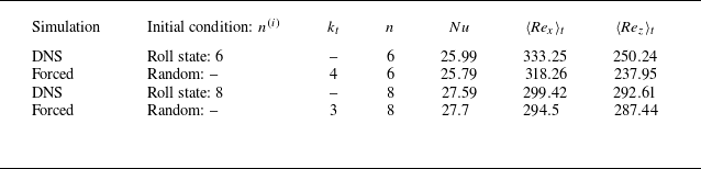
combination without depending on initial conditions. The converged statistics from the simulations presented in figures 5 and 6 are tabulated in table 1. The statistics, especially
$[Ra, Pr]$
combination without depending on initial conditions. The converged statistics from the simulations presented in figures 5 and 6 are tabulated in table 1. The statistics, especially
 $Nu$
from the forced simulations, are in very good agreement with the DNS (these results are also in agreement with those reported by Wang et al. Reference Wang, Verzicco, Lohse and Shishkina2020). The maximum deviation of the reported Reynolds numbers is within
$Nu$
from the forced simulations, are in very good agreement with the DNS (these results are also in agreement with those reported by Wang et al. Reference Wang, Verzicco, Lohse and Shishkina2020). The maximum deviation of the reported Reynolds numbers is within
 $5\,\%$
.
$5\,\%$
.
Table 1. Details of direct and forced simulations to capture multiple states for
 $[Ra, Pr]=[10^8, 10]$
. Here,
$[Ra, Pr]=[10^8, 10]$
. Here,
 $k_t$
is the integer streamwise wavenumber for forcing.
$k_t$
is the integer streamwise wavenumber for forcing.
What happens if both states (
 $n=8$
and
$n=8$
and
 $6$
) are suppressed? Figure 7 shows an instantaneous snapshot of
$6$
) are suppressed? Figure 7 shows an instantaneous snapshot of
 ${\mathcal{T}}$
from a forced simulation with
${\mathcal{T}}$
from a forced simulation with
 $k_t=[3, 4]$
at
$k_t=[3, 4]$
at
 $t/t_f= 150$
. While at this
$t/t_f= 150$
. While at this
 $t/t_f$
, forcing with either
$t/t_f$
, forcing with either
 $k_t=4$
or
$k_t=4$
or
 $k_t=3$
in figure 6 yields the
$k_t=3$
in figure 6 yields the
 $n=6$
or 8 state, respectively, for
$n=6$
or 8 state, respectively, for
 $k_t=[3, 4]$
the proposed technique does not yield a state with convection rolls of regular shape and size. Although plumes are visible, arbitrary patterns emerge without any regular shape.
$k_t=[3, 4]$
the proposed technique does not yield a state with convection rolls of regular shape and size. Although plumes are visible, arbitrary patterns emerge without any regular shape.
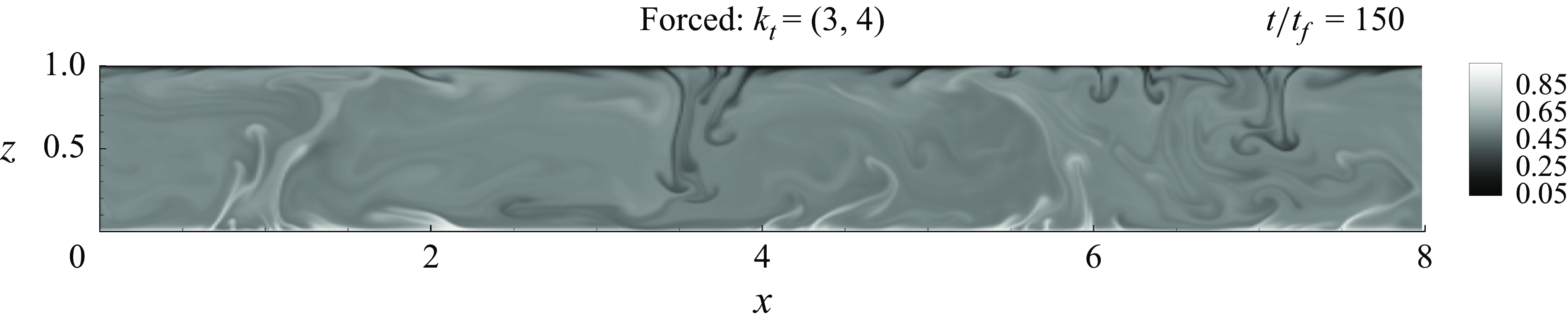
Figure 7. Instantaneous snapshot of
 ${\mathcal{T}}$
at
${\mathcal{T}}$
at
 $t/t_f=150$
from a forced simulation with
$t/t_f=150$
from a forced simulation with
 $k_t=[3, 4]$
for
$k_t=[3, 4]$
for
 $[Ra, Pr]=[10^8, 10]$
.
$[Ra, Pr]=[10^8, 10]$
.
3.2. Multiple states for
$[Ra, Pr]=[10^9, 3]$

For
 $[Ra, Pr]=[10^9, 3]$
, Wang et al. (Reference Wang, Verzicco, Lohse and Shishkina2020) reported three states with different mean aspect ratios:
$[Ra, Pr]=[10^9, 3]$
, Wang et al. (Reference Wang, Verzicco, Lohse and Shishkina2020) reported three states with different mean aspect ratios:
 $n=8$
(
$n=8$
(
 $\Gamma _r=1$
),
$\Gamma _r=1$
),
 $n=10$
(
$n=10$
(
 $\Gamma _r=4/5$
) and
$\Gamma _r=4/5$
) and
 $n=12$
(
$n=12$
(
 $\Gamma _r=2/3$
) convection rolls were obtained in a computational domain with aspect ratio
$\Gamma _r=2/3$
) convection rolls were obtained in a computational domain with aspect ratio
 $\Gamma =8$
. The results for these multiple states are presented in figures 8 and 9.
$\Gamma =8$
. The results for these multiple states are presented in figures 8 and 9.
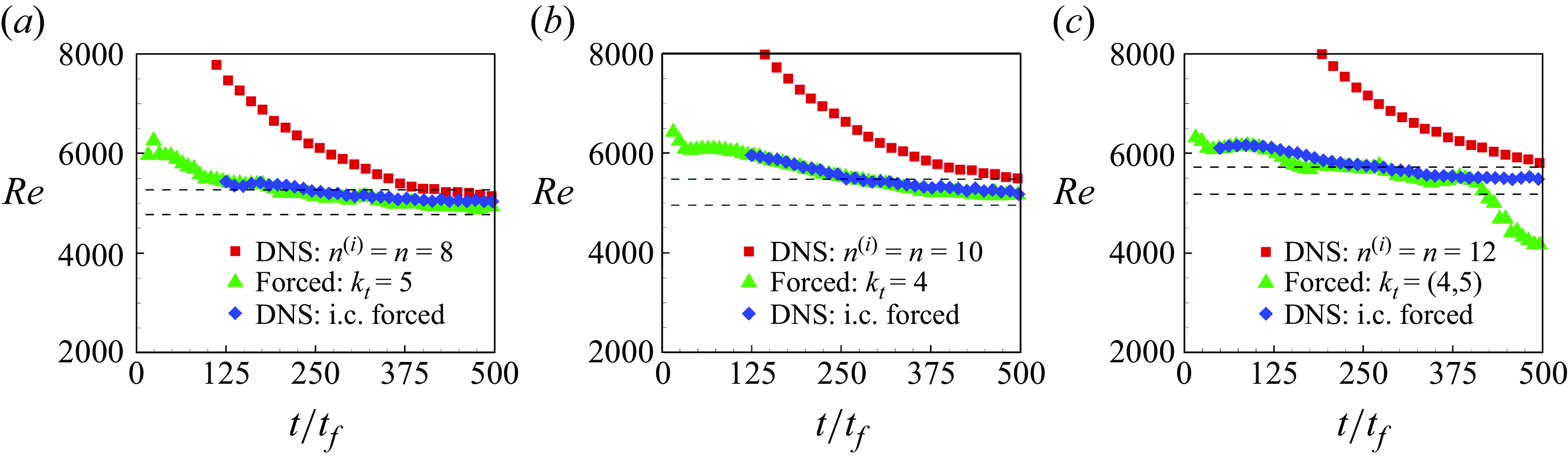
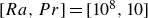
Figure 8. Plots of
 $\textit{Re}$
as a function of simulation time (
$\textit{Re}$
as a function of simulation time (
 $t/t_f$
) for
$t/t_f$
) for
 $[Ra, Pr]=[10^9, 3]$
: (
$[Ra, Pr]=[10^9, 3]$
: (
 $a$
) simulations yielding the
$a$
) simulations yielding the
 $n=8$
roll state, (
$n=8$
roll state, (
 $b$
) simulations yielding the
$b$
) simulations yielding the
 $n=10$
roll state, (
$n=10$
roll state, (
 $c$
) simulations yielding the
$c$
) simulations yielding the
 $n=12$
roll state. The cases are: DNS initiated with
$n=12$
roll state. The cases are: DNS initiated with
 $n^{(i)}=n$
(red squares), forced simulation with
$n^{(i)}=n$
(red squares), forced simulation with
 $k_t$
(green triangles), and switching off the forcing (blue diamonand switching off the forcing (blue diamonds). The horizontal dashed lines correspond to
$k_t$
(green triangles), and switching off the forcing (blue diamonand switching off the forcing (blue diamonds). The horizontal dashed lines correspond to
 $\pm 5\,\%$
of the
$\pm 5\,\%$
of the
 $\textit{Re}$
values reported by Wang et al. (Reference Wang, Verzicco, Lohse and Shishkina2020) from their DNS. i.c. is initial condition.
$\textit{Re}$
values reported by Wang et al. (Reference Wang, Verzicco, Lohse and Shishkina2020) from their DNS. i.c. is initial condition.
Figure 9. Instantaneous snapshots of
 ${\mathcal{T}}$
from (a,c,e) DNS initiated with
${\mathcal{T}}$
from (a,c,e) DNS initiated with
 $n^{(i)}=n=8, 10, 12$
, respectively, at chosen
$n^{(i)}=n=8, 10, 12$
, respectively, at chosen
 $t/t_f$
, and (b,d,f) forced simulations with
$t/t_f$
, and (b,d,f) forced simulations with
 $k_t=5, 4, [4,5]$
, respectively, at chosen
$k_t=5, 4, [4,5]$
, respectively, at chosen
 $t/t_f$
.
$t/t_f$
.
Figure 8(
 $a$
) shows the convergence of
$a$
) shows the convergence of
 $\textit{Re}$
as a function of the simulation time
$\textit{Re}$
as a function of the simulation time
 $t/t_f$
for DNS initiated with
$t/t_f$
for DNS initiated with
 $n^{(i)}=8=n$
, a forced simulation with
$n^{(i)}=8=n$
, a forced simulation with
 $k_t=5$
(suppressing emergence of
$k_t=5$
(suppressing emergence of
 $n=10$
roll state), and essentially another DNS switching off the forcing at
$n=10$
roll state), and essentially another DNS switching off the forcing at
 $t/t_f=125$
. Figures 9(a,b) show how the flow structures by plotting the instantaneous contours of
$t/t_f=125$
. Figures 9(a,b) show how the flow structures by plotting the instantaneous contours of
 ${\mathcal{T}}$
from the DNS and the forced simulation at
${\mathcal{T}}$
from the DNS and the forced simulation at
 $t/t_f=68$
and 67, respectively. Clearly, the forced simulation with
$t/t_f=68$
and 67, respectively. Clearly, the forced simulation with
 $k_t=5$
has been able to capture the state with
$k_t=5$
has been able to capture the state with
 $n=8$
. In addition, starting from a random initial condition, the statistics converge much more quickly using the forcing technique in comparison to the DNS. Ideally, the forcing should be switched off once a roll state is obtained using the proposed method. Here, in figure 8(
$n=8$
. In addition, starting from a random initial condition, the statistics converge much more quickly using the forcing technique in comparison to the DNS. Ideally, the forcing should be switched off once a roll state is obtained using the proposed method. Here, in figure 8(
 $a$
), the result is also shown after the forcing is switched off at
$a$
), the result is also shown after the forcing is switched off at
 $t/t_f=125$
once the
$t/t_f=125$
once the
 $n=8$
state is obtained in the forced simulation (blue diamond symbols). In these DNS, the
$n=8$
state is obtained in the forced simulation (blue diamond symbols). In these DNS, the
 $n=8$
state obtained using the forcing was found to sustain itself even after the forcing was switched off (not shown here).
$n=8$
state obtained using the forcing was found to sustain itself even after the forcing was switched off (not shown here).
Suppression of the
 $n=8$
state using
$n=8$
state using
 $k_t=4$
, on the other hand, yields the
$k_t=4$
, on the other hand, yields the
 $n=10$
state with
$n=10$
state with
 $\Gamma _r=4/5$
. The results from this forced simulation along with DNS initiated with
$\Gamma _r=4/5$
. The results from this forced simulation along with DNS initiated with
 $n^{(i)}=10$
are shown in figures 8(
$n^{(i)}=10$
are shown in figures 8(
 $b$
), 9(
$b$
), 9(
 $c$
) and 9(
$c$
) and 9(
 $d$
). Figure 8(
$d$
). Figure 8(
 $b$
) shows again that the convergence to a statistically stationary state is much slower in the DNS compared to the proposed method. The forcing technique yields the convection rolls as early as
$b$
) shows again that the convergence to a statistically stationary state is much slower in the DNS compared to the proposed method. The forcing technique yields the convection rolls as early as
 $t/t_f=51$
in figure 9(
$t/t_f=51$
in figure 9(
 $d$
). The forcing was switched off at
$d$
). The forcing was switched off at
 $t/t_f=125$
in more DNS reported in figure 8(
$t/t_f=125$
in more DNS reported in figure 8(
 $b$
). The
$b$
). The
 $n=10$
state was able to sustain itself in these DNS (not shown here).The
$n=10$
state was able to sustain itself in these DNS (not shown here).The
 $\textit{Re}$
statistics from this simulation are almost identical to that from the forced simulation, demonstrating the efficacy of the forcing methodology.
$\textit{Re}$
statistics from this simulation are almost identical to that from the forced simulation, demonstrating the efficacy of the forcing methodology.
Suppression of both
 $n=8$
and
$n=8$
and
 $n=10$
roll states is necessary to yield the
$n=10$
roll states is necessary to yield the
 $n=12$
roll state using the proposed method. The results for the roll state
$n=12$
roll state using the proposed method. The results for the roll state
 $n=12$
are presented in figures 8(
$n=12$
are presented in figures 8(
 $c$
), 9(
$c$
), 9(
 $e$
) and 9(
$e$
) and 9(
 $f$
). The instantaneous snapshots of
$f$
). The instantaneous snapshots of
 ${\mathcal{T}}$
from DNS initiated with
${\mathcal{T}}$
from DNS initiated with
 $n^{(i)}=12$
, and a forced simulation with
$n^{(i)}=12$
, and a forced simulation with
 $k_t=[4, 5]$
(all triad interactions mediated by wavenumbers corresponding to
$k_t=[4, 5]$
(all triad interactions mediated by wavenumbers corresponding to
 $\Gamma _r=1$
and
$\Gamma _r=1$
and
 $4/5$
are removed), are shown in figures 9(
$4/5$
are removed), are shown in figures 9(
 $e$
) and 9(
$e$
) and 9(
 $f$
), respectively. Although initialised with a random condition, the proposed forcing technique captures the
$f$
), respectively. Although initialised with a random condition, the proposed forcing technique captures the
 $n=12$
state quickly, as early as
$n=12$
state quickly, as early as
 $t/t_f=51$
, as shown in figure 9(
$t/t_f=51$
, as shown in figure 9(
 $f$
). In comparison, as reflected in the contour plot in figure 9(
$f$
). In comparison, as reflected in the contour plot in figure 9(
 $e$
), and also for
$e$
), and also for
 $\textit{Re}$
plotted against
$\textit{Re}$
plotted against
 $t/t_f$
in figure 8(
$t/t_f$
in figure 8(
 $c$
), the convergence of DNS initiated with
$c$
), the convergence of DNS initiated with
 $n^{(i)}=12$
is much slower. Figure 8(
$n^{(i)}=12$
is much slower. Figure 8(
 $c$
) also includes results from DNS after the forcing was switched off at
$c$
) also includes results from DNS after the forcing was switched off at
 $t/t_f=50$
. The
$t/t_f=50$
. The
 $n=12$
state yielded with forcing is also able to sustain itself in these DNS (not shown here). Over the course of the simulation,
$n=12$
state yielded with forcing is also able to sustain itself in these DNS (not shown here). Over the course of the simulation,
 $\textit{Re}$
plotted for this simulation is also in agreement with the forced simulation.
$\textit{Re}$
plotted for this simulation is also in agreement with the forced simulation.
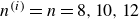
For this
 $[Ra, Pr]$
combination, a forced simulation was performed suppressing known multiple states (
$[Ra, Pr]$
combination, a forced simulation was performed suppressing known multiple states (
 $n=8, 10, 12$
in a
$n=8, 10, 12$
in a
 $\Gamma =8$
computational domain). For this simulation, we chose
$\Gamma =8$
computational domain). For this simulation, we chose
 $k_t=[4, 5, 6]$
(wavenumbers corresponding to the multiple states). The long-time solution converges to a statistically stationary
$k_t=[4, 5, 6]$
(wavenumbers corresponding to the multiple states). The long-time solution converges to a statistically stationary
 $n=6$
state (see figure 10). However, the obtained
$n=6$
state (see figure 10). However, the obtained
 $n=6$
state transitioned to the
$n=6$
state transitioned to the
 $n=8$
state once the forcing was switched off (not shown here). Therefore, the proposed method can possibly lead to states that are not stable in DNS. The unphysical nature of the forcing is aggravated as more and more triad interactions are removed, or in other words, the size of the subspace,
$n=8$
state once the forcing was switched off (not shown here). Therefore, the proposed method can possibly lead to states that are not stable in DNS. The unphysical nature of the forcing is aggravated as more and more triad interactions are removed, or in other words, the size of the subspace,
 $k_t$
, is increased. In essence, with increase in the size of the subspace
$k_t$
, is increased. In essence, with increase in the size of the subspace
 $k_t$
, the nonlinearity of the system is increasingly restricted. A forced simulation yields the most stable state (as the initial condition is ‘random’) of the system of equations (with restricted nonlinearity) solved that is not necessarily stable for the fully nonlinear system. The forcing terms in (2.14) and (2.15) might remove triad interactions that might otherwise be necessary for the sustenance of a state. Although the proposed method can yield the flow states and the associated statistics accurately enough to be compared with those obtained from DNS, the proposed methodology is reliant on DNS for verification purposes.
$k_t$
, the nonlinearity of the system is increasingly restricted. A forced simulation yields the most stable state (as the initial condition is ‘random’) of the system of equations (with restricted nonlinearity) solved that is not necessarily stable for the fully nonlinear system. The forcing terms in (2.14) and (2.15) might remove triad interactions that might otherwise be necessary for the sustenance of a state. Although the proposed method can yield the flow states and the associated statistics accurately enough to be compared with those obtained from DNS, the proposed methodology is reliant on DNS for verification purposes.
Figure 10. Instantaneous snapshot of
 ${\mathcal{T}}$
at
${\mathcal{T}}$
at
 $t/t_f=500$
from the forced simulation with
$t/t_f=500$
from the forced simulation with
 $k_t=[4, 5, 6]$
for
$k_t=[4, 5, 6]$
for
 $[Ra, Pr]=[10^9, 3]$
.
$[Ra, Pr]=[10^9, 3]$
.
3.3. Practical applications of the forcing technique
The proposed method may be used to uncover the multiple convection roll states in 2-D RBC. The steps involved are as follows. (i) Perform DNS with the random initial condition to converge to a roll state (the characteristic wavenumber associated with the captured mean roll size is
 $k_1$
, say). (ii) Perform simulation using the proposed forcing technique with
$k_1$
, say). (ii) Perform simulation using the proposed forcing technique with
 $k_t=[k_1, \ldots ]$
to test if another roll state (with characteristic wavenumber
$k_t=[k_1, \ldots ]$
to test if another roll state (with characteristic wavenumber
 $k_2$
, say) can be obtained. If a new state cannot be obtained, all possible states have been discovered. (iii) If another roll state is obtained, then switch off the forcing to check if the obtained state sustains in DNS. (iv) If the new roll state sustains itself in DNS, then increase the size of the subspace to
$k_2$
, say) can be obtained. If a new state cannot be obtained, all possible states have been discovered. (iii) If another roll state is obtained, then switch off the forcing to check if the obtained state sustains in DNS. (iv) If the new roll state sustains itself in DNS, then increase the size of the subspace to
 $k_t=[k_1, k_2, \ldots ]$
, and repeat step (ii). Otherwise, if the roll state transitions back to one of the already discovered states, then all multiple states have been obtained.
$k_t=[k_1, k_2, \ldots ]$
, and repeat step (ii). Otherwise, if the roll state transitions back to one of the already discovered states, then all multiple states have been obtained.
Additionally, the proposed methodology can empirically designatethe stability of each of the multiple states. Ideally, the emergence of a more stable state should require suppression of a lesser number of candidate wavenumbers. The most stable state should emerge without forcing from a random initial condition, followed by other lesser stable states, with the removal of more and more triads mediated by candidate wavenumbers. When all possible multiple states are ruled out using the forcing technique, the consequent restricted nonlinearity of the governing equations may yield highly unstable states that are otherwise unlikely to emerge for the fully nonlinear system (see Bose et al. Reference Bose, Kannan and Zhu2024).
We emphasise that the proposed method could possibly be used to compute the different states in other flow configurations where multiple states exist for a set of control parameters. The continuation based methods (Dijkstra et al. Reference Dijkstra2014) can yield a superposition of multiple states at such a point in the bifurcation diagram, while only one of the states is obtained as the solution is continued along a branch. On the other hand, the present method should be able to capture the multiple states as discrete solutions at such a point in the bifurcation diagram, provided that the wavenumbers associated with the dominant flow structures mediate energy in triad interactions. The investigation of such possibilities remains an open question.
4. Conclusions
In this paper, a new methodology is proposed to obtain the multiple convection roll states in 2-D RBC flow. For the same control parameters
 $[Ra, Pr]$
, convection rolls with different aspect ratios (
$[Ra, Pr]$
, convection rolls with different aspect ratios (
 $\Gamma _r$
) emerge yielding different statistically stationary states; in previous works, the selection of
$\Gamma _r$
) emerge yielding different statistically stationary states; in previous works, the selection of
 $\Gamma _r$
was dependent on
$\Gamma _r$
was dependent on
 $\Gamma _r$
of rolls in the initial condition. Using the methodology proposed in this paper, the possible multiple states for any
$\Gamma _r$
of rolls in the initial condition. Using the methodology proposed in this paper, the possible multiple states for any
 $[Ra, Pr]$
combination can be captured exhaustively, circumventing the issues related to the dependence of the emergence of the states on initial conditions.
$[Ra, Pr]$
combination can be captured exhaustively, circumventing the issues related to the dependence of the emergence of the states on initial conditions.
In the proposed method, forcing terms are prescribed that remove select nonlinear triadic scale interactions from the OBEs (2.1)–(2.3). This is motivated by the observation that the characteristic horizontal wavenumber associated with the mean size of the convection rolls (
 $k_r$
) mediates temperature variance and kinetic energy transfer processes in triad interactions at a statistically stationary state establishing cascade processes (figures 1 and 2). The participating wavenumbers in such triads are of the form
$k_r$
) mediates temperature variance and kinetic energy transfer processes in triad interactions at a statistically stationary state establishing cascade processes (figures 1 and 2). The participating wavenumbers in such triads are of the form
 $[k, p, m=k-p=\pm k_r]$
, where,
$[k, p, m=k-p=\pm k_r]$
, where,
 $k$
,
$k$
,
 $p$
and
$p$
and
 $m$
are the receiver, donator and mediator wavenumbers, respectively. Herein, we prescribed the forcing terms in (2.14) and (2.15), leveraging this information to remove triad interactions that are mediated by one/multiple target wavenumbers,
$m$
are the receiver, donator and mediator wavenumbers, respectively. Herein, we prescribed the forcing terms in (2.14) and (2.15), leveraging this information to remove triad interactions that are mediated by one/multiple target wavenumbers,
 $k_t=[k_1, k_2, \ldots ]$
. Removing such triad interactions physically suppresses the emergence of the convection rolls with characteristic wavenumbers
$k_t=[k_1, k_2, \ldots ]$
. Removing such triad interactions physically suppresses the emergence of the convection rolls with characteristic wavenumbers
 $k_t$
. As a consequence, roll formation is encouraged at another candidate wavenumber that does not belong to
$k_t$
. As a consequence, roll formation is encouraged at another candidate wavenumber that does not belong to
 $k_t$
, which is therefore allowed to mediate energy among triads and establish the essential cascade processes.
$k_t$
, which is therefore allowed to mediate energy among triads and establish the essential cascade processes.
The proposed forcing technique is used to obtain the multiple states in a computational domain with aspect ratio
 $\Gamma =8$
for two cases –
$\Gamma =8$
for two cases –
 $[Ra, Pr]=[10^8, 10]$
and
$[Ra, Pr]=[10^8, 10]$
and
 $[10^9, 3]$
. For both these cases, the multiple states could be yielded from a ‘random’ initial condition that does not include any signature of the final roll state. For comparison, we also perform DNS initialised from momentum fields bearing the signature of the target roll states (2.8) and (2.9). The two possible states for
$[10^9, 3]$
. For both these cases, the multiple states could be yielded from a ‘random’ initial condition that does not include any signature of the final roll state. For comparison, we also perform DNS initialised from momentum fields bearing the signature of the target roll states (2.8) and (2.9). The two possible states for
 $[Ra, Pr]=[10^8, 10]$
are captured by suppressing in each case the mediation of energy by one of the candidate wavenumbers for roll formation (figures 5 and 6). Additionally, the statistics obtained from the forced simulations are in good agreement with the statistics obtained from the DNS (table 1). Removing the triad interactions mediated by both candidate wavenumbers does not capture any roll state with a regular pattern (figure 7). All three multiple states could also be captured for
$[Ra, Pr]=[10^8, 10]$
are captured by suppressing in each case the mediation of energy by one of the candidate wavenumbers for roll formation (figures 5 and 6). Additionally, the statistics obtained from the forced simulations are in good agreement with the statistics obtained from the DNS (table 1). Removing the triad interactions mediated by both candidate wavenumbers does not capture any roll state with a regular pattern (figure 7). All three multiple states could also be captured for
 $[Ra, Pr]=[10^9, 3]$
– suppression of only one candidate wavenumber was sufficient to yield two of the multiple states. The
$[Ra, Pr]=[10^9, 3]$
– suppression of only one candidate wavenumber was sufficient to yield two of the multiple states. The
 $n=8$
state could be captured suppressing the emergence of
$n=8$
state could be captured suppressing the emergence of
 $n=10$
state, and vice versa (figures 8(a,b) and 9(
$n=10$
state, and vice versa (figures 8(a,b) and 9(
 $a$
–
$a$
–
 $d$
)). However, to capture the
$d$
)). However, to capture the
 $n=12$
state, candidate wavenumbers corresponding to both
$n=12$
state, candidate wavenumbers corresponding to both
 $n=8$
and
$n=8$
and
 $n=10$
states had to be forced out (figures 8(
$n=10$
states had to be forced out (figures 8(
 $c$
) and 9(
$c$
) and 9(
 $e$
,
$e$
,
 $f$
)). All the multiple states captured using the proposed method were found to sustain themselves in direct simulations after the forcing was switched off. If all three states are suppressed, then the forcing technique yields an
$f$
)). All the multiple states captured using the proposed method were found to sustain themselves in direct simulations after the forcing was switched off. If all three states are suppressed, then the forcing technique yields an
 $n=6$
state – a state that was found to transition to the
$n=6$
state – a state that was found to transition to the
 $n=8$
state once the forcing was switched off. Specifically, for
$n=8$
state once the forcing was switched off. Specifically, for
 $[Ra, Pr]=[10^9, 3]$
, the forcing technique converges to the statistically stationary states much more quickly than in DNS initiated with the signature of the target states.
$[Ra, Pr]=[10^9, 3]$
, the forcing technique converges to the statistically stationary states much more quickly than in DNS initiated with the signature of the target states.
It has been demonstrated that the proposed methodology could be utilised to uncover all possible multiple roll states in 2-D RBC efficiently. The possible states obtained by the forcing technique, while ‘stable’ for the forced system of equations, are not necessarily stable for the original unforced system of equations (e.g. the
 $n=6$
state obtained for the forced system for
$n=6$
state obtained for the forced system for
 $[Ra, Pr]=[10^9, 3]$
). The proposed forcing method yields a roll state quickly, irrespective of the initial condition; the forced simulations also approach statistical stationarity much more quickly. In addition, the proposed method can designate each state with respect to its stability and in comparison to other states. However, it must be noted that despite capturing the states quickly, this method is reliant on the direct simulation for verification, as ultimately it uses manipulation of the triadic scale interactions, which are unphysical in nature. Even if a state appears stable under the forced equations, DNS must be run with that state as the initial condition to verify its true stability. We believe that the proposed method should be able to discretely capture the multiple states in other flow configurations in both non-turbulent and turbulent regimes provided that the dominant flow structures mediate energy in triadic scale interactions.
$[Ra, Pr]=[10^9, 3]$
). The proposed forcing method yields a roll state quickly, irrespective of the initial condition; the forced simulations also approach statistical stationarity much more quickly. In addition, the proposed method can designate each state with respect to its stability and in comparison to other states. However, it must be noted that despite capturing the states quickly, this method is reliant on the direct simulation for verification, as ultimately it uses manipulation of the triadic scale interactions, which are unphysical in nature. Even if a state appears stable under the forced equations, DNS must be run with that state as the initial condition to verify its true stability. We believe that the proposed method should be able to discretely capture the multiple states in other flow configurations in both non-turbulent and turbulent regimes provided that the dominant flow structures mediate energy in triadic scale interactions.
Funding
We gratefully acknowledge financial support from the Max Planck Society, the German Research Foundation (DFG), from grants 521319293, 540422505 and 550262949. We also thank the HPC systems of Max Planck Computing and Data Facility (MPCDF) for the allocation of computational time.
Declaration of interests
The authors report no conflict of interest.
Data availability statement
The data that support the findings of this study will be available upon reasonable request.


 Open access