2. Problem setting

A fully developed longitudinal flow in a channel with periodic fins is considered. Per above, the fin spacing is defined by $S^*$, the height of the fins is $H^*$, and the clearance is $c^*$. The dimensional flow is unidirectional, with velocity $w^*(x^*,y^*)$ in the $Z^*$ direction satisfying

(2.1)\begin{equation} \frac{\partial^2 w^*}{\partial x^{*2}} + \frac{\partial^2 w^*}{\partial y^{*2}} = \frac{1}{\mu}\,\frac{\partial p^*}{\partial Z^*}, \quad (x^*,y^*) \in D^*, \end{equation}

in a period window $D^*\equiv \{(x^*,y^*)\,|\, 0\leq x^*\leq S^*,\ 0\leq y^*\leq H^* + c^* \}$, and driven by a constant pressure gradient $-\partial p^*/\partial Z^*$. The fluid viscosity is $\mu$. The no-slip condition holds on the shroud, fins and base (referred to as the prime surface in the heat transfer literature), i.e.

(2.2)$$\begin{gather} w^*(x^*,0) = w^*(x^*,H^*+c^*) = 0,\quad 0\leq x^*\leq S^*, \end{gather}$$

(2.3)$$\begin{gather}w^*(0,y^*) = w^*(S^*,y^*) = 0,\quad 0\leq y^* \leq H^*. \end{gather}$$

Because of the periodicity, we can impose symmetry conditions along the remaining parts of the boundary above the fin tips, i.e.

(2.4)\begin{equation} \frac{\partial w^*}{\partial x^*}(0,y^*) = \frac{\partial w^*}{\partial x^*}(S^*,y^*) = 0,\quad H^*< y^* \leq H^*+c^*. \end{equation}

As mentioned above, we scale lengths with the fin height $H^*$, so the non-dimensional coordinates are given by

(2.5)\begin{equation} (x,y,Z) = \frac{1}{H^*}\,(x^*,y^*,Z^*), \end{equation}

and we define a non-dimensional velocity

(2.6)\begin{equation} w =-\frac{\mu}{H^{*2}}\left(\frac{\partial p^*}{\partial Z^*}\right)^{-1} w^*. \end{equation}

As in Sparrow et al. (Reference Sparrow, Baliga and Patankar1978), we assume that the thickness of the fins is negligible compared to $H^*$, $c^*$ and $S^*$. The non-dimensional parameters are, as per above, defined by $\epsilon \equiv S^*/H^*$ and $c \equiv c^*/H^*$, which represent the ratio of fin spacing to fin height and clearance to fin height, respectively. The non-dimensional period window is hence given by $D=\{(x,y) \,|\, 0\leq x \leq \epsilon,\ 0\leq y \leq 1+c\}$, and since the domain is symmetric about the centreline $x=\epsilon /2$, we denote one half of $D$ corresponding to $0\leq x \leq \epsilon /2$ by $D_{half}$. The geometry is shown in figure 1(b). The non-dimensional flow $w(x,y)$ then satisfies

(2.7)\begin{equation} \frac{\partial^2 w}{\partial x^2} + \frac{\partial^2 w}{\partial y^2} =-1,\quad (x,y) \in D, \end{equation}

with no-slip conditions

(2.8)$$\begin{gather} w(x,0) = w(x,1+c) =0,\quad 0\leq x \leq \epsilon, \end{gather}$$

(2.9)$$\begin{gather}w(0,y) = w(\epsilon,y)=0,\quad 0\leq y \leq 1, \end{gather}$$

and symmetry conditions

(2.10)\begin{equation} \frac{\partial w}{\partial x}(0,y) = \frac{\partial w}{\partial x}(\epsilon,y) = 0,\quad 1\leq y \leq 1+c.\end{equation}

After solving the above problem for the velocity $w(x,y)$ in $D$, the friction factor times the Reynolds number of the channel is calculated by Sparrow et al. (Reference Sparrow, Baliga and Patankar1978) as

(2.11)\begin{equation} f\,{Re} \equiv \frac{8}{w_{m}}\left(\frac{(1+c)\epsilon}{1+\epsilon}\right)^2, \end{equation}

where $w_{m}$ is the mean velocity in the period window $D$, i.e.

(2.12)\begin{equation} w_{m} \equiv \frac{1}{\epsilon(1+c)}\int_D w(x,y)\, {\rm d}\kern0.06em x\,{\rm d} y. \end{equation}

We note that the foregoing formula from Sparrow et al. (Reference Sparrow, Baliga and Patankar1978) are consistent with their conventional definitions of Reynolds number, equivalent diameter and friction factor.

Sparrow et al. (Reference Sparrow, Baliga and Patankar1978) used the finite difference method to calculate the velocity field, and obtained $f\,{Re}$ for a limited set of discrete values of $\epsilon$ and $c$. The main contribution of this paper is to derive exact and accurate explicit asymptotic formulae for (2.11) to allow the easy computation for a wide range of $\epsilon$ and $c$. Next, we summarize these new formulae for $f\,{Re}$ in § 3, and provide their derivations in §§ 5–7.

3. Summary of new formulae for $f\,{Re}$

This section summarizes and discusses the contributions of this paper: formulae for $f\,{Re}$ with no clearance ($c=0$), and formulae with finite clearance ($c>0$). The latter includes a new exact formula and various asymptotic formulae for small $\epsilon$ and/or $c$.

3.1. No clearance ($c=0$)

3.1.1. Exact formula

When there is no clearance, the flow in a period window corresponds to the classical case of flow through a rectangular duct. There is an exact series solution derived in the context of elasticity by Timoshenko & Goodier (Reference Timoshenko and Goodier1970) and reported for fluid flow by e.g. Shah & London (Reference Shah and London1978). We derive a different (and convenient for our purposes) representation for this solution in terms of complex variables. The velocity profile is given by

(3.1)\begin{equation} w(x,y) = w_{P,0}(x,y) + \hat{w}_P(x,y),\end{equation}

where

(3.2a,b)$$\begin{gather} w_{P,0}(x,y) \equiv \frac{x(\epsilon- x)}{2},\quad \hat{w}_P(x,y) = {\rm Im}[g(z;0)], \end{gather}$$

(3.3)$$\begin{gather}g(z;\alpha) \equiv-\sum_{n=1,3,\ldots}^\infty \frac{4\epsilon^2}{{\rm \pi}^3 n^3 (1+{\rm e}^{-n{\rm \pi}(1+\alpha)/\epsilon})}\,( {\rm e}^{n{\rm \pi}{\rm i} z/\epsilon} - {\rm e}^{-n{\rm \pi}(1 +\alpha+{\rm i} z)/\epsilon}), \end{gather}$$

and $z=x+{\rm i} y$. The function $g(z;\alpha )$ is also used to construct the exact solution for the case $c>0$ in § 6. The friction factor times the Reynolds number is calculated by the definition (2.11) and an application of Green's second identity as per Appendix B. Recall, the notation $f\,{Re}$ is used here to represent the friction factor times the Reynolds number, which is calculated by the explicit expression for the mean velocity given by (3.9) with $c=0$.

3.1.2. Case $\epsilon \ll 1$

For $\epsilon \ll 1$ with $c=0$, corresponding to a small ratio of fin spacing to height (or a small-aspect-ratio rectangular duct), $f\,{Re}$ can be approximated by

(3.4)\begin{equation} f\,{Re}_{asymp} \sim \frac{96}{\left(1-\beta\epsilon+\dfrac{384\epsilon}{{\rm \pi}^5}\,({\rm e}^{-{\rm \pi}/\epsilon}-{\rm e}^{-2{\rm \pi}/\epsilon}) \right)(1+\epsilon)^2} + O(\epsilon\, {\rm e}^{-3{\rm \pi}/\epsilon}), \end{equation}

where $\beta =(186/{\rm \pi} ^5)\,\tilde {\zeta }(5) \approx 0.6302$, and $\tilde {\zeta }(5)$ is the Riemann zeta function evaluated at 5. The derivation of this expression is explained in § 7.

Figure 2 shows the comparison between the exact solution and the asymptotic one, (3.4). We also compare (3.4) with a fitted polynomial expression for $f\,{Re}$ when $c=0$ that is commonly used in the literature (Shah & London Reference Shah and London1978):

(3.5)\begin{equation} f\,{Re}_{poly} \approx 96(1-1.3553\epsilon+1.9467\epsilon^2 - 1.7012 \epsilon^3 + 0.9564 \epsilon^4 - 0.2537 \epsilon^5). \end{equation}

Even though the new formula (3.4) was derived assuming $\epsilon \ll 1$, since the error term is exponentially small in $\epsilon$, it shows extraordinary accuracy when compared to the exact solution over the entire range $0\leq \epsilon \leq 1$, as shown in figure 2. The new formula contains no infinite sum, and the relative error is less than $10^{-4}$, even lower than for the polynomial fit (3.5), which was fit to the exact solution over the entire range $0\leq \epsilon \leq 1$.

Figure 2.

(a) Plots of $f\,{Re}$ versus $\epsilon$ when $c=0$ (i.e. flow in a rectangular duct). (b) Log–log plot of the errors (relative to the exact solution) of the asymptotic expression (3.4) and the polynomial expression (3.5).

3.2. Finite clearance ($c>0$)

For the case of finite (non-zero) clearance, we present an exact solution derived using complex conformal mapping techniques, and three simpler asymptotic solutions in several different limits of $\epsilon$ and $c$.

3.2.1. Exact formula

The exact expression for the flow is derived by splitting $w(x,y)$ into $w_P(x,y)$, which is the flow in a no-slip rectangular duct of width $\epsilon$ and height $1+c$, and a correction term $\hat {w}(x,y)$. That is,

(3.6)\begin{equation} w(x,y) = w_P(x,y) + \hat{w}(x,y), \end{equation}

with (cf. (3.1)–(3.3))

(3.7)\begin{equation} w_P(x,y) = w_{P,0}(x,y) + \hat{w}_P(x,y), \end{equation}

where $\hat {w}_P={\rm Im}[g(z;c)]$ and the correction $\hat {w}(x,y)$ is found to be (see the detailed derivation in § 6)

(3.8)\begin{equation} \hat{w}(x,y) = {\rm Im}\left[\frac{1}{2{\rm \pi} {\rm i}}\oint_{C_0}\phi(\zeta')\,[ {\rm d}\log \omega(\zeta',\zeta) + {\rm d}\log \overline{\omega}(\overline{\zeta'},1/\zeta) ]\right], \end{equation}

where $z = {\mathcal {Z}}(\zeta )$ is a conformal map from the upper left unit circle, excluding a smaller inner circle, to the half period window $D_{half}$, as discussed in § 6, and $\phi (\zeta )$ is a known real function that ensures that the boundary condition (2.10) is satisfied by the full solution (3.6). Here, $\omega ({\cdot },{\cdot })$ is the prime function (Crowdy Reference Crowdy2020) of the triply connected domain illustrated in the right-hand part of figure 10(b).

After calculating the field $w(x,y)$, it is straightforward to obtain the friction factor times the Reynolds number of the channel. Using the reciprocity theorem proposed by Crowdy (Reference Crowdy2017) (i.e. Green's second identity), the mean velocity of $w(x,y)$ in the period window $D$ can be calculated from knowledge of $\hat {w}(x,y)$ on the symmetry boundary only:

(3.9)\begin{align} w_{m} &= \frac{\epsilon^2}{12} - \frac{1}{1+c}\sum_{n=1,3,\ldots}^\infty \frac{16\epsilon^3}{{\rm \pi}^5 n^5 }\tanh\left(\frac{n{\rm \pi} (1+c)}{2\epsilon} \right)\nonumber\\ &\quad +\frac{1}{1+c}\int_{1}^{1+c}\left(1-\sum_{n=1,3,\ldots}^\infty \frac{8({\rm e}^{-n{\rm \pi} y/\epsilon} + {\rm e}^{n{\rm \pi}(y-1-c)/\epsilon})}{{\rm \pi}^2n^2 (1+{\rm e}^{-n{\rm \pi}(1+c)/\epsilon})}\right)\hat{w}(0,y)\,{\rm d} y. \end{align}

The derivation is explained in detail in Appendix B. Using (3.9), $f\,{Re}$ then follows from its definition, (2.11). Some numerical results for $f\,{Re}$ for a range of $\epsilon$ and $c$ values are plotted in figure 3, and shown to agree with the numerical results of Sparrow et al. (Reference Sparrow, Baliga and Patankar1978). The small differences are attributed to an insufficient number of mesh points by Sparrow et al. (Reference Sparrow, Baliga and Patankar1978) due to computational limitations.

Figure 3.

Friction factor times Reynolds number plotted against $\epsilon$ for various choices of clearance $c$, using the exact solution (3.9) and (2.11). Also plotted are the values calculated by Sparrow et al. (Reference Sparrow, Baliga and Patankar1978).

3.2.2. Case (1): $\epsilon \ll 1$, $\epsilon \ll c$

This case corresponds to the case where the fin spacing is small compared to both the fin height and clearance, i.e. $\epsilon \ll 1$ and $\epsilon \ll c$. The flow behaviour becomes significantly different in different parts of the domain, and the method of matched asymptotic expansions can be employed. The main contribution to the mean flow comes from the clearance region above the fins, with a correction due to the flow field near the fin tips. The resulting $f\,{Re}$ formula is given by

(3.10)\begin{equation} f\,{Re}_{(1)} \sim \frac{96(1+c)^3\epsilon^2}{\displaystyle{ c^2\left(c + \dfrac{\epsilon \log 8}{\rm \pi}\right)(1+\epsilon)^2 }} + O(\epsilon^4),\quad \epsilon \ll1. \end{equation}

The detailed derivation is given in § 7. It is compared to the exact solution at the end of this section in figures 4 and 5.

Figure 4.

The relative error calculated by (3.13) for cases (1), (2) and (3). Solid lines and dashed lines correspond to the boundaries of the 1 % and 15 % errors, respectively. A solid line and dashed line exist in the yellow-shaded region of case (2), because the results given by the asymptotics are coincidentally close to the exact $f\,{Re}$.

Figure 5.

(a) Illustration of the regions in which the errors defined by (3.13) are less than $15\,\%$. Almost all regions are covered by the asymptotics $f\,{Re}_{(1)}$, $f\,{Re}_{(2)}$ and $f\,{Re}_{(3)}$. (b) Illustration of the regions in which the errors defined by (3.13) are less than $1\,\%$.

3.2.3. Case (2): $c\ll \epsilon \ll 1$

This case corresponds to the case where the clearance is small compared to the fin spacing ($c\ll \epsilon$), which in turn is small compared to the fin height ($\epsilon \ll 1)$. This is similar to case (1) in that $\epsilon \ll 1$, but here we consider $c \ll \epsilon$, which is the reverse of (and hence complementary to) case (1), where $c \gg \epsilon$. In this case, a different matched asymptotic expansion is considered, leading to the following formula for $f\,{Re}$:

(3.11)\begin{align} &f\,{Re}_{(2)} \nonumber\\ &\quad \sim \dfrac{96(1+c)^3}{\left[1+c-\epsilon\left(\beta - \dfrac{384}{{\rm \pi}^5}\,({\rm e}^{-{\rm \pi}(1+c)/\epsilon}-{\rm e}^{-2{\rm \pi}(1+c)/\epsilon}) - \dfrac{3c^4}{{\rm \pi}\epsilon^4}\left(\log\left(\dfrac{2\epsilon}{{\rm \pi} c}\right) + \dfrac{3}{2}\right)^2 \right) \right](1+\epsilon)^2}\nonumber\\ &\qquad+ O\left(\epsilon \left(\frac{c}{\epsilon}\right)^4\log \left(\frac{c}{\epsilon}\right)\right) + O(\epsilon\, {\rm e}^{-3{\rm \pi}/\epsilon}), \end{align}

where $\beta$ is the same constant as defined in (3.4). This formula is derived in § 7. We have included two error terms in (3.11), which are due to the two separate approximations $\epsilon \ll 1$ and $c\ll \epsilon$. Note that this formula reduces to the asymptotic formula (3.4) when $c=0$, therefore this is a generalization of that approximation to $0\leq c \ll \epsilon$.

3.2.4. Case (3): $c\lesssim \epsilon \ll 1$

This case is similar to case (2) but is shown to be accurate for a wider range of $\epsilon$ and $c$, at a slight increase in complexity. In this case, the clearance $c$ is assumed to be comparable in size to the spacing $\epsilon$, which is small. Then only a detailed solution in the clearance region is necessary. Using another (but simpler) conformal mapping approach to that used in (3.8), the flow $\hat {w}(x,y)$ in (3.6) on the symmetry line ($x=0$, $1\leq y \leq 1+c$) is approximated by

(3.12)\begin{align} \hat{w}(0,y) \sim \hat{A} \left[1 - \frac{(1+\cosh^{1/2}({\rm \pi} c/\epsilon))^2}{(1-\cosh^{1/2}({\rm \pi} c/\epsilon))^2}\times \frac{(\cosh({\rm \pi}(y-1-c)/\epsilon)-\cosh^{1/2}({\rm \pi} c/\epsilon))^2}{(\cosh({\rm \pi}(y-1-c)/\epsilon)+\cosh^{1/2}({\rm \pi} c/\epsilon))^2}\right]^{1/2}, \end{align}

where $\hat {A}$ is a parameter calculated by a Fourier integral. Although (3.12) is valid only on $x=0$, $1\leq y\leq 1+c$, it is sufficient to calculate the mean velocity using the reciprocity result (3.9). Then $f\,{Re}$ follows from the definition (2.11). The notation $f\,{Re}_{(3)}$ represents the friction factors times the Reynolds number that is calculated by this method.

3.2.5. Comparison of cases (1), (2) and (3)

These three expressions (3.10), (3.11) and (3.12) for cases (1), (2) and (3), respectively, are compared with $f\,{Re}$ calculated by the exact formula (3.6) for a representative range of $\epsilon$ and $c$ in figure 4. The relative error is defined by (where $k$ is the case number)

(3.13)\begin{equation} {\rm Error}(\,f\,{Re}_{(k)}) \equiv \frac{|\,f\,{Re} - f\,{Re}_{(k)}|}{f\,{Re}},\quad k = 1,2,3. \end{equation}

Solid lines and dashed lines correspond to the boundaries of the 1 % and 10 % errors, respectively.

The three cases are combined in figures 5(a,b), which show the regions where the errors (3.13) between analytical formulae and asymptotics formulae are less than $15\,\%$ and 1 %, respectively. Together, almost all of the region considered ($0.01\leq c$, $\epsilon \leq 1$) is covered by the formulae for cases (1), (2) and (3). Only in the white region, where all asymptotic formulae show an error >15 % (or >1 %), must the exact complex variable solution be used.

4. Illustrative results

Using (3.6)–(3.8), representative contour plots of the non-dimensional velocity $w(x,y)$ for (a) $\epsilon=0.5$, $c=0$, (b) $\epsilon=0.3$, $c=0.1$, (c) $\epsilon=0.4$, $c=0.2$, (d) $\epsilon=0.5$, $c=1$, and (e) $\epsilon=0.25$, $c=1$ are illustrated in figure 6. When $c = 0$, the highest velocity is in the centre of the domain. This is approximately true at the low clearances in figures 6(b,c), i.e. $c = 0.1$ ($\epsilon = 0.3$) and $c = 0.2$ ($\epsilon = 0.4)$, respectively. However, when the clearance is the same as the fin height ($c = 1$) in figure 6(d) for $\epsilon = 0.5$ and figure 6(e) for $\epsilon = 0.25$, the highest velocity is about midway between the fin tips and shroud. Also, in figures 6(c,d,e), when $c$ is 0.2 or larger, the velocity is, essentially, dependent upon $y$ only sufficiently close to the shroud. This is not true, of course, regardless of $\epsilon$, when $c=0$ (figure 6a) and does not apply for $c=0.1$ ($\epsilon = 0.3$) (figure 6b). As discussed below, for $\epsilon \ll 1$, $\epsilon \ll c$, the flow is parabolic in $x$ between the fins, and parabolic in $y$ above them, except in an intermediate (overlap) region near the fin tips and an unimportant region near the base.

Figure 6.

Representative contour plots of the non-dimensional velocity $w(x,y)$, using the exact solution (3.6)–(3.8), for (a) $\epsilon =0.5$, $c=0$, (b) $\epsilon =0.3$, $c=0.1$, (c) $\epsilon =0.4$, $c=0.2$, (d) $\epsilon =0.5$, $c=1$, and (e) $\epsilon =0.25$, $c=1$.

Figure 7 plots, as a function of $y$, the ratio of the mean velocity over the width of the domain, $\bar {w}(y)$, to that for the entire domain, $w_{m}$. When $c=0.1$ ($\epsilon = 0.3$) (figure 7b), most of the total flow is between the fins, and when $c=0.2$ ($\epsilon = 0.4$) (figure 7c), this is still true. Conversely, when, $c=1$, a small fraction of the total flow is between the fins, especially as $\epsilon$ is reduced from 0.5 (figure 7d) to 0.25 (figure 7e).

Figure 7.

Mean velocity over domain width, $\bar {w}(y)$, divided by the mean velocity over domain, $w_{m}$, i.e. $(1+c)\int _{0}^{\epsilon }w(x,y)\,{\rm d}\kern0.06em x/\int _{D} w(x,y)\,{\rm d}\kern0.06em x\,{\rm d} y$, as a function of $y$ for (a) $\epsilon =0.5$, $c=0$, (b) $\epsilon =0.3$, $c=0.1$, (c) $\epsilon =0.4$, $c=0.2$, (d) $\epsilon =0.5$, $c=1$, and (e) $\epsilon =0.25$, $c=1$.

Figure 8 plots the ratio of the local shear stress along the fin (upper row), base (middle row) and shroud (top row) to the mean shear stress along the wetted perimeter of the domain for cases (a)–(e). When $c=0$, the maximum local shear stress along each of the three surfaces is at its centre. When $c$ is finite, however, this is true along the base and shroud but not the fin. Indeed, there is a square root singularity in shear stress as the tip of the fin is approached. The shear stress along the base is weakest when $c = 1$ in figures 8(d,e), when a small fraction of the total flow is between the fins. When $c=0.2$ and higher (figures 8c)–(e), the local shear stress is essentially constant along the shroud. Sparrow et al. (Reference Sparrow, Baliga and Patankar1978) provides analogous plots for the heat transfer problem.

Figure 8.

Ratio of the local shear stress (i.e. $\tau = \partial w/\partial n$, where $n$ is the normal direction pointing into the domain) on the fin, base and shroud to the mean shear stress along the wetted perimeter of the domain, $\tau _{m}$, i.e. $\int (\partial w/\partial n)\, {\rm d}s \times 1/(2+2\epsilon )$, for (a) $\epsilon =0.5$, $c=0$, (b) $\epsilon =0.3$, $c=0.1$, (c) $\epsilon =0.4$, $c=0.2$, (d) $\epsilon =0.5$, $c=1$, and (e) $\epsilon =0.25$, $c=1$.

5. Derivation of an analytical formula for $f\,{Re}$ when $c=0$

For $c=0$, the flow in a channel corresponds to the flow in a rectangular duct. The flow in a rectangular duct is itself important. This formula is classical and already derived in the context of the theory of elasticity by Timoshenko & Goodier (Reference Timoshenko and Goodier1970) (see Shah & London Reference Shah and London1978). Crowdy also found an explicit solution for $w_P(x,y)$ by using a conformal map from an annular region (see p. 326 in Crowdy Reference Crowdy2020). The derivation is explained here again through complex analysis techniques to make the paper self-contained, and the result will be used to derive the flow with the finite clearance.

Here, we follow the approach proposed by Crowdy (Reference Crowdy2020). The analytical formula for the flow can be derived by splitting $w(x,y)$ into $w_{P,0}(x,y)$ and $\hat {w}_{P}(x,y)$ defined in (3.1). The function $\hat {w}_P$ is harmonic in $D$ and satisfies the boundary conditions

(5.1)$$\begin{gather} \hat{w}_P(x,0) = \hat{w}_P(x,1) =-\frac{x(\epsilon-x)}{2},\quad \text{on} \ 0\leq x \leq \epsilon, \end{gather}$$

(5.2)$$\begin{gather}\hat{w}_P(0,y) = \hat{w}_P(\epsilon,y)= 0,\quad \text{on}\ 0\leq y \leq 1. \end{gather}$$

Now consider the conformal maps

(5.3a,b)\begin{equation} \xi = \varTheta(z)= \exp\left(\frac{{\rm \pi} {\rm i} z}{\epsilon} \right),\quad z = {\mathcal{T}}(\xi) = \frac{\epsilon}{{\rm \pi}{\rm i} }\log \xi, \end{equation}

where ${\mathcal {T}}(\xi )$ maps to the whole period window $D$ from the upper half-annulus with the inner radius $q = \exp (-{\rm \pi} /\epsilon )$ in the $\xi$-plane. The map is illustrated in figure 9. Note that the bottom wall $0\leq x\leq \epsilon$, $y=0$ is mapped to the upper semicircle of $C_0$ defined by $C_0^+$, and the upper wall $0\leq x\leq \epsilon$, $y=1$ is mapped to the upper semicircle of $C_1$ with the radius $q$ defined by $C_1^+$.

Figure 9.

Conformal mapping from the annular region to the whole period window $D$.

Now consider $g(z;0) \equiv \chi _P+{\rm i} \hat {w}_P$ and $G(\xi )\equiv g({\mathcal {T}}(\xi );0)$. Because of the boundary condition (5.1), the function $G(\xi )$ satisfies the following boundary conditions on $C_0^+$ and $C_1^+$:

(5.4)\begin{equation} G(\xi) =-\frac{{\rm Re}[{\mathcal{T}}(\xi)]\,(\epsilon - {\rm Re}[{\mathcal{T}}(\xi)]) }{2},\quad \xi \in C_0^+, C_1^+. \end{equation}

Also, because of the boundary condition (5.2) and the map (5.3),

(5.5)\begin{equation} {\rm Im}[G(\xi)] = \frac{1}{2{\rm i}}\,(G(\xi) - \overline{G(\xi)}) = 0,\quad \overline{\xi} = \xi. \end{equation}

By using the Schwarz reflection principle, the function $G(\xi )$ is extended to the lower half-disc outside of the inner circle, and satisfies

(5.6)\begin{equation} \overline{G}(\xi) = G(\xi), \end{equation}

for the whole unit disc outside the inner circle $C_1$. Using (5.6) the function $G(\xi )$ satisfies

(5.7)\begin{equation} {\rm Im}[G(\xi)]=-{\rm Im}[\overline{G(\xi)}]=-{\rm Im}[G(\overline{\xi})],\quad \xi \in C_0^-, C_1^-, \end{equation}

where $C_0^-$ and $C_1^-$ are the lower semicircles of $C_0$ and $C_1$. Due to (5.4), (5.7) and the property that ${\rm arg}(\overline {\xi })=-{\rm arg}(\xi )$, the function $G(\xi )$ then satisfies the boundary conditions

(5.8)\begin{equation} {\rm Im}[G(\xi)] = \left\{\begin{array}{@{}ll} -\dfrac{\epsilon^2 \,{\rm arg}(\xi)\,(1-{\rm arg}(\xi)/{\rm \pi})}{2{\rm \pi}}, & \xi \in C_0^+, C_1^+,\\ -\dfrac{\epsilon^2 \,{\rm arg}(\xi)\,(1+{\rm arg}(\xi)/{\rm \pi})}{2{\rm \pi}}, & \xi \in C_0^-, C_1^-. \end{array}\right. \end{equation}

This can be solved by the Fourier–Laurent series expression. Let

(5.9)\begin{equation} G(\xi) = c_0 +\sum_{n=1}^\infty (c_n \xi^n + c_{-n} \xi^{-n}),\quad c_n, c_{-n}\in \mathbb{R}, \end{equation}

where the fact that $c_{n},c_{-n}\in \mathbb {R}$ comes from ${\rm Im}[G(\xi )]= 0$ on $\overline {\xi }=\xi$. From (5.8), ${\rm Im}[G(\xi )]={\rm Im}[G(q \xi )]$ for $\xi \in C_0$, which means that the coefficients $c_n$, $n\in \mathbb {N}$, should satisfy the special relations $c_{-n} = -q^{n} c_{n}$, $n=1,\ldots,\infty$. These coefficients can be determined by the Fourier sine series representation of the boundary values:

(5.10)\begin{equation} {\rm Im}[{G}({\rm e}^{{\rm i}\theta})] = \sum_{n=1}^{\infty} c_n(1+q^{n})\sin n\theta = b_0(\theta), \end{equation}

where the boundary condition (5.8) is now $b_0(\theta )$ expressed in terms of $\theta$:

(5.11)\begin{equation} b_0(\theta) \equiv \left\{\begin{array}{@{}ll} -\dfrac{\epsilon^2 \theta(1-\theta/{\rm \pi})}{2{\rm \pi}}, & 0\leq\theta\leq {\rm \pi},\\ -\dfrac{\epsilon^2 \theta(1+\theta/{\rm \pi})}{2{\rm \pi}}, & -{\rm \pi}\leq\theta\leq 0. \end{array}\right. \end{equation}

The coefficients $c_n$ can be obtained by the standard Fourier integral:

(5.12)\begin{equation} c_n =-\frac{2\epsilon^2 (1-(-1)^n)}{{\rm \pi}^3 (1+q^n) n^3},\quad n=1,\ldots, \infty, \end{equation}

where we have used the relation

(5.13)\begin{equation} \int_{0}^{\rm \pi} \theta({\rm \pi}-\theta)\sin n\theta\, {\rm d}\theta + \int_{-{\rm \pi}}^{0} \theta ({\rm \pi}+\theta)\sin n\theta \,{\rm d}\theta = \frac{4(1-(-1)^n)}{n^3}. \end{equation}

By substituting the original Laurent expression (5.9),

(5.14)\begin{equation} {G}(\xi) =-\sum_{n=1,3,\ldots}^\infty \frac{4\epsilon^2}{{\rm \pi}^3 n^3 (1+q^n)}\,( \xi^n - q^n \xi^{-n} ). \end{equation}

Using the conformal map $\xi =\varTheta (z)$ defined by (5.3), the final formula (3.3) is derived.

6. Derivation of analytical formulae for $f\,{Re}$ when $c>0$

Here, a complex analysis formulation for the exact solution when $c>0$ given in (3.6)–(3.8) is introduced. The flow $w(x,y)$ is decomposed into the flow in a rectangular duct and a flow harmonic in $D$ as follows:

(6.1)\begin{equation} w(x,y) = w_P(x,y) + \hat{w}(x,y), \end{equation}

where $w_P(x,y)$ is a pressure-driven flow in a rectangular duct, as already given in the previous section,

(6.2)\begin{equation} w_P(x,y) = w_{P,0}(x,y) + \hat{w}_{P}(x,y), \end{equation}

with $\hat {w}_P(x,y)\equiv {\rm Im}[g(z;c)]$. This decomposition is illustrated in figure 10(a).

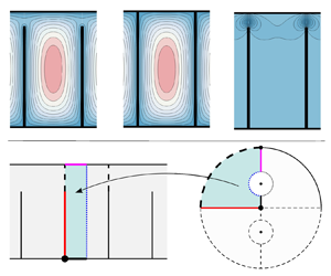
Figure 10.

(a) Periodic channel flow $w(x,y)$ and its decomposition $w_P(x,y)$ and $\hat {w}(x,y)$. (b) Conformal mapping from the upper left domain $D_\zeta ^{-+}$ to the half-period window of $D$.

Now consider the function $\hat {w}(x,y)$ that is harmonic in the half-period window $D_{half}$. The function $\hat {w}(x,y)$ satisfies

(6.3)$$\begin{gather} \hat{w}(0,y) = 0,\quad 0\leq y \leq 1, \end{gather}$$

(6.4)$$\begin{gather}\hat{w}(x,0)=\hat{w}(x,1+c) = 0,\quad 0\leq x \leq \epsilon/2, \end{gather}$$

(6.5)$$\begin{gather}\frac{\partial \hat{w}}{\partial x}(\epsilon/2,y) = 0,\quad 0\leq y \leq 1+c, \end{gather}$$

where the last condition comes from the periodicity of the channel. Because of the symmetry condition (2.10), $\hat {w}(x,y)$ should satisfy

(6.6)\begin{align} \frac{\partial w}{\partial x}(0,y)&=\frac{\partial \hat{w}}{\partial x}(0,y) + \frac{\partial w_P}{\partial x} (0,y)\nonumber\\ &=\frac{\partial \hat{w}}{\partial x}(0,y)+\frac{\partial \hat{w}_P}{\partial x} (0,y)+\frac{\epsilon}{2}=0,\quad 1\leq y \leq 1+c. \end{align}

Because $\hat {w}(x,y)$ is a harmonic function in $D_{half}$, it is convenient to define $h(z) \equiv \chi + {\rm i} \hat {w}$, where $\chi$ is a harmonic conjugate of $\hat {w}$. From (6.5) and use of the Cauchy–Riemann equations.

(6.7)\begin{equation} \frac{\partial \hat{w}}{\partial x}(\epsilon/2,y) =-\frac{\partial \chi}{\partial y}(\epsilon/2,y) = 0,\quad 0\leq y\leq 1+c. \end{equation}

This means that $\chi (\epsilon /2,y)$ is constant on $0\leq y \leq 1+c$, so it is convenient to set $\chi (\epsilon /2,y)=0$ for $0\leq y \leq 1+c$, without loss of generality. In addition, the condition (6.6) and use of the Cauchy–Riemann equations again give

(6.8)\begin{equation} \frac{\partial \chi}{\partial y}(0,y) =-\frac{\partial \hat{w}}{\partial x}(0,y) = \frac{\partial \hat{w}_P}{\partial x}(0,y) +\frac{\epsilon}{2}=-\frac{\partial \chi_P}{\partial y}(0,y) + \frac{\epsilon}{2}, \quad 1\leq y \leq 1+c,\end{equation}

where $\chi _P(x,y)\equiv {\rm Re}[g(z;c)]$. Integrating (6.8) from $1$ to $y$ gives

(6.9)\begin{align} \chi(0,y) - \chi_0 &=-(\chi_P(0,y)-\chi_P(0,1))+\frac{\epsilon}{2}\,(y-1) \nonumber\\ &=-{\rm Re}[g({\rm i} y;c)-g({\rm i};c)] + \frac{\epsilon}{2}\,(y-1), \quad \chi_0\equiv \chi(0,1)\in\mathbb{R}. \end{align}

Now we introduce the conformal mapping to the half-period window $D_{half}$ in the $z$-plane from $D_\zeta ^{-+}$, which is defined by the upper left unit quarter-disc outside an inner small circle $C_1$ in the complex $\zeta$-plane. This map is defined by

(6.10)\begin{equation} z = {\mathcal{Z}}(\zeta) \equiv-\frac{1+c}{\rm \pi}\log \left(\frac{\omega(\zeta,\theta_1(\infty))}{\omega(\zeta,\theta_2(\infty))}\right) + (1+c){\rm i}, \end{equation}

where

(6.11a,b)\begin{equation} \theta_1(\zeta) \equiv \delta + \frac{q^2}{1-\overline{\delta}\zeta},\quad \theta_2(\zeta)\equiv-\delta + \frac{q^2}{1+\overline{\delta}\zeta}. \end{equation}

The function ${\mathcal {Z}}(\zeta )$ maps the negative real axis to $\{(x,y)\,|\,x=0,\ 0\leq y \leq 1\}$, the upper left circle $C_0^{-+}$ to the gap $\{(x,y)\,|\,x=0,\ 1\leq y \leq 1+c\}$, and the left-hand side of the inner circle $C_1^-$ to $\{(x,y)\,|\,x=\epsilon /2,\ 0\leq y \leq 1+c\}$, respectively. The map is visualized in figure 10(b). The same map was used to solve flows through a channel involving superhydrophobic surfaces with invaded grooves (Miyoshi et al. Reference Miyoshi, Rodriguez-Broadbent, Curran and Crowdy2022).

It is convenient to define ${\mathcal {H}}(\zeta ) \equiv h({\mathcal {Z}}(\zeta ))$. The boundary condition (6.9) becomes

(6.12)\begin{equation} {\rm Re}[{\mathcal{H}}(\zeta)] =-{\rm Re}[g({\mathcal{Z}}(\zeta);c)-g({\rm i};c)] + \frac{\epsilon}{2}\,({\rm Im}[{\mathcal{Z}}(\zeta)]-1) + \chi_0,\quad \zeta \in C_0^{-+}. \end{equation}

On the imaginary axis of the domain $D_\zeta ^{-+}$, $\hat {w}(x,y)=0$ from (6.4), which means that

(6.13)\begin{equation} {\rm Im}[{\mathcal{H}}(\zeta)] = \frac{1}{2{\rm i}}\,({\mathcal{H}}(\zeta) - \overline{{\mathcal{H}}(\zeta)}) = \frac{1}{2{\rm i}}\,({\mathcal{H}}(\zeta) - \overline{{\mathcal{H}}}(-\zeta)) = 0, \end{equation}

where we have used the fact that $\overline {\zeta } = -\zeta$ on the imaginary axis. By the Schwarz reflection principle, the function ${\mathcal {H}}(\zeta )$ can be analytically continued to the right-hand half-disc outside $C_1$ defined by $D_\zeta ^{++}$, and satisfies

(6.14) \begin{equation} {\mathcal{H}}(\zeta) = \overline{{\mathcal{H}}(-\overline{\zeta})} = \overline{{\mathcal{H}}}(-\zeta),\quad \zeta \in D_\zeta^{++}. \end{equation}

Using the fact that $\chi =0$ on $0\leq y\leq 1+c$ because of (6.7), which means ${\rm Re}[{\mathcal {H}}(\zeta )]=0$ on $\zeta \in C_1$, ${\rm Re}[\zeta ]<0$, we have

(6.15)\begin{equation} {\rm Re}[{\mathcal{H}}(\zeta)] ={\rm Re}[\overline{{\mathcal{H}}(\zeta)}]= {\rm Re}[{\mathcal{H}}(-\overline{\zeta})]=0,\quad \zeta \in C_1,\ {\rm Re}[\zeta] > 0. \end{equation}

On the negative real axis of the domain $D_\zeta ^{-+}$, ${\rm Im}[{\mathcal {H}}(\zeta )]=0$ from (6.3). On the positive real axis of $D_\zeta ^{++}$, the use of (6.14) and (6.3) gives

(6.16)\begin{equation} {\rm Im}[{\mathcal{H}}(\zeta)] = {\rm Im}[\overline{{\mathcal{H}}(-\overline{\zeta})}] =-{\rm Im}[{\mathcal{H}}(-\overline{\zeta})] =-{\rm Im}[{\mathcal{H}}(-\zeta)] = 0, \end{equation}

where we have used the fact that $\overline {\zeta }=\zeta$ on the real axis. Hence ${\rm Im}[{\mathcal {H}}(\zeta )]=0$ on the real axis of $D_\zeta ^{++}\cup D_\zeta ^{-+}$. By the Schwarz reflection principle again, the function ${\mathcal {H}}(\zeta )$ can be continued to the lower half-disc outside the inner circle $C_2$, which is the reflection of $C_1$ in the real axis. The lower half-disc outside $C_2$ is defined by $D_\zeta ^-\equiv D_\zeta ^{+-}\cup D_\zeta ^{--}$. The function ${\mathcal {H}}(\zeta )$ then satisfies

(6.17)\begin{equation} {\mathcal{H}}(\zeta) =\overline{{\mathcal{H}}(\overline{\zeta})} = \overline{{\mathcal{H}}}(\zeta),\quad \zeta \in D_\zeta^-. \end{equation}

Thus, the function ${\mathcal {H}}(\zeta )$ is analytically continued to the whole unit disc outside $C_1$ and $C_2$, and satisfies the boundary conditions

(6.18)\begin{equation} {\rm Re}[{\mathcal{H}}(\zeta)] =\left\{\begin{array}{@{}ll} \phi(\zeta), & \zeta \in C_0,\\[2pt] 0, & \zeta \in C_1,C_2,\\ \end{array}\right. \end{equation}

where

(6.19)\begin{equation} \phi(\zeta) = \left\{\begin{array}{@{}ll} -{\rm Re}[g({\mathcal{Z}}(-\zeta);c) - g({\rm i};c)] & \\ \quad +\ \dfrac{\epsilon}{2}\,({\rm Im}[{\mathcal{Z}}(-\zeta)]-1) + \chi_0, & \zeta \in C_0^{++},C_0^{+-},\\ - {\rm Re}[g({\mathcal{Z}}(\zeta);c) - g({\rm i};c)] & \\ \quad +\ \dfrac{\epsilon}{2}\,({\rm Im}[{\mathcal{Z}}(\zeta)]-1) + \chi_0, & \zeta \in C_0^{-+},C_0^{--}, \end{array}\right. \end{equation}

where the property ${\mathcal {Z}}(\overline {\zeta }) = {\mathcal {Z}}(\zeta )$ for $\zeta \in C_0$ has been used. This boundary value problem can be solved by the standard Schwarz integral proposed by Crowdy (Reference Crowdy2020) (see also Crowdy Reference Crowdy2008) as follows:

(6.20)\begin{equation} {\mathcal{H}}(\zeta) = \frac{1}{2{\rm \pi} {\rm i}}\oint_{C_0}\phi(\zeta')\,[{\rm d}\log \omega(\zeta',\zeta) + {\rm d}\log \overline{\omega}(\overline{\zeta'},1/\zeta) ] +{\rm i} \hat{c}_0,\quad \hat{c}_0\in \mathbb{R}, \end{equation}

where $\hat {c}_0$ is determined by the condition $w(0,0)=0$, and it has been confirmed numerically that $\hat {c}_0=0$. The constant $\chi _0$ should be calculated beforehand, and it is easily obtained by the single-valuedness condition on ${\mathcal {H}}(\zeta )$ around $C_1$ and $C_2$ (Crowdy Reference Crowdy2020). By combining (6.1) with (6.20), expression (3.6) is obtained.

The general theory of the prime function can be found in Crowdy (Reference Crowdy2020). It is an important special function that can be associated with any multiply connected circular domain. To evaluate (6.20), it is necessary to be able to evaluate the prime function $\omega ({\cdot },{\cdot })$. Appendix A explains how to evaluate the function in detail.

One of the advantages of using our method is the elimination of square root singularities at the apexes of the fins, namely, at $x=0$ and $y=1$. As detailed in § 6, the solution is obtained via the Schwarz integral of continuous boundary values, ensuring the absence of singularities along the integration path. Further insights into these singularities are provided in Miyoshi et al. (Reference Miyoshi, Rodriguez-Broadbent, Curran and Crowdy2022).

Finally, it should be mentioned that there is another approach to solving this boundary value problem that uses a doubly connected concentric annulus rather than a triply connected circular domain. That approach follows a formulation by Marshall (Reference Marshall2017), who found the solution for flow in a superhydrophobic channel with patterning on the upper and lower walls. Readers interested in a discussion of the relationship between these methods are referred to Miyoshi et al. (Reference Miyoshi, Rodriguez-Broadbent, Curran and Crowdy2022).

7. Derivation of asymptotic approximations for $f\,{Re}$

This section provides the derivations of asymptotic approximations for $f\,{Re}$ when $\epsilon \ll 1$, and for various assumptions on the clearance $c$. We first consider the flow problem (2.7)–(2.10) in the geometric limit $\epsilon \ll 1$ when $c=0$. Then for the finite clearance case, i.e. $c>0$, three cases are considered: (1) the fin spacing is small compared to the fin height and clearance; (2) the clearance is small compared to the fin spacing, which is small compared to the fin height; (3) the same as case (2) but valid for larger ratios of clearance to fin spacing, i.e. up to ratios of unity.

Mathematically, we proceed by first considering the limit where the fin spacing is small in comparison to the fin height, i.e. $\epsilon \ll 1$. Then we will consider the three distinct cases for different sizes of the tip clearance $c$. These cases are $c=0$ (no tip clearance), $c\gg \epsilon$ and $c \lesssim \epsilon$.

7.1. No clearance – case $\epsilon \ll 1$

When $c=0$, a convenient approximation for the mean velocity for $\epsilon \to 0$ can be derived directly from (3.9). Setting $c=0$, (3.9) reduces to the solution (Shah & London Reference Shah and London1978)

(7.1)\begin{equation} w_{m} = \frac{\epsilon^2}{12} - \frac{16\epsilon^3}{{\rm \pi}^5}\sum_{n=1,3,\ldots}^\infty \frac{1}{n^5}\tanh\left(\frac{n{\rm \pi}}{2\epsilon}\right). \end{equation}

When $\epsilon \to 0$, $\tanh (n{\rm \pi} /2\epsilon )=1-2\,{\rm e}^{-n{\rm \pi} /\epsilon }+2\,{\rm e}^{-2n{\rm \pi} /\epsilon }+O({\rm e}^{-3{\rm \pi} /\epsilon })$, so we have

(7.2)\begin{align} w_{m} &\sim \frac{\epsilon^2}{12} - \frac{16\epsilon^3}{{\rm \pi}^5}\sum_{n={1,3,\ldots}}^\infty\frac{1}{n^5}\,(1-2\,{\rm e}^{-n{\rm \pi}/\epsilon} + 2\,{\rm e}^{-2n{\rm \pi}/\epsilon})+O(\epsilon^3 \,{\rm e}^{-3{\rm \pi}/\epsilon}) \end{align}

(7.3)\begin{align} &\sim\frac{\epsilon^2}{12} - \frac{16\epsilon^3}{{\rm \pi}^5}\left(\frac{31}{32}\,\tilde{\zeta}(5)-2\,{\rm e}^{-{\rm \pi}/\epsilon}+2\,{\rm e}^{-2{\rm \pi}/\epsilon}\right) +O(\epsilon^3 \,{\rm e}^{-3{\rm \pi}/\epsilon}) \end{align}

(7.4)\begin{align} &=\frac{\epsilon^2}{12}\left(1-\beta\epsilon+\dfrac{384\epsilon}{{\rm \pi}^5}\,({\rm e}^{-{\rm \pi}/\epsilon}-{\rm e}^{-2{\rm \pi}/\epsilon})\right)\nonumber\\ &\quad +O(\epsilon^3\,{\rm e}^{-3{\rm \pi}/\epsilon}),\quad \beta=\frac{186}{{\rm \pi}^5}\,\tilde{\zeta}(5) \equiv 0.6302\ldots, \end{align}

as $\epsilon \rightarrow 0$, and $\tilde {\zeta }(5)$ is the Riemann zeta function evaluated at 5. Thus we can arrive at the asymptotic formula for $f\,{Re}$ when $c=0$, which is given by (3.4). The consideration of three terms in the expansion of ${\rm tanh}(n{\rm \pi} /2\epsilon )$ was chosen to give the right balance between accuracy over the range $0\leq \epsilon \leq 1$, and the complexity of the formula.

7.2. Finite clearance – case (1): $\epsilon \ll c$, $\epsilon \ll 1$

For this case, we construct a solution directly using matched asymptotic expansions. It is convenient to rescale the $x$ coordinate by defining $X=x/\epsilon$, so that the problem domain is independent of $\epsilon$. Then (2.7)–(2.10) become

(7.5)$$\begin{gather} \frac{1}{\epsilon^2}\,\frac{\partial^2 w}{\partial X^2} + \frac{\partial^2 w}{\partial y^2} =-1 \quad \text{in } D_w=\{0< X<1, 0< y<1+c\}, \end{gather}$$

(7.6)$$\begin{gather}w = 0 \quad \text{on } y=0,\ 1 + c, \end{gather}$$

(7.7)$$\begin{gather}w = 0 \quad \text{on } X=0,1,\ 0< y < 1, \end{gather}$$

(7.8)$$\begin{gather}\frac{\partial w}{\partial X} = 0 \quad \text{on } X = 0,1,\ 1< y < 1+c. \end{gather}$$

Considering now $\epsilon \to 0$, the asymptotic solution takes a different form depending on the region in the domain. Employing matched asymptotic expansions, we decompose the domain into a gap region ($1 < y < 1 + c$) above the fins, a fin region ($0 < y < 1$) between the fins, and a short ‘tip region’ near the fin tips ($y - 1 = O(\epsilon )$) that transitions between them. See figure 11 for a schematic of this domain decomposition. The boundaries between these regions will be handled carefully in the following subsections.

Figure 11.

Asymptotic structure of the domain showing the gap, tip and fin regions, and the behaviour of the velocity in each region (the region close to the base, $y=O(\epsilon )$, is not considered here).

7.2.1. Gap region: $1 < y < 1 + c$

First, we consider a regular expansion in powers of $\epsilon$,

(7.9)\begin{equation} w(X,y) = w_0 + \epsilon w_1 + \epsilon^2 w_2 + O(\epsilon^3),\quad \epsilon \to 0, \end{equation}

which, when substituted into (7.5), gives $w_0 = A_0(y)\,X + B_0(y)$ at leading order in $\epsilon$, i.e. $O(\epsilon ^{-2})$. Applying the symmetry conditions (7.8) above the fins gives $A_0(y)\equiv 0$, i.e. $w_0 = w_0(y)$. Considering (7.5) at $O(\epsilon ^{-1})$, we similarly find $w_1 = w_1(y)$. Hence the leading-order balance is at $O(1)$,

(7.10)\begin{equation} \frac{\partial^2 w_2}{\partial X^2} + \frac{\mathrm{d}^2 w_0}{\mathrm{d} y^2} =-1, \end{equation}

which, integrating over $0< X<1$ and applying the symmetry conditions $\partial w_2 / \partial X = 0$ at $X=0, 1$, yields

(7.11)\begin{equation} \frac{\mathrm{d}^2 w_0}{\mathrm{d} y^2} =-1. \end{equation}

Integrating and applying the no-slip condition on the shroud, $y=1+c$, we arrive at

(7.12)\begin{equation} w_0(y) = \tfrac{1}{2}(1+c)^2 - \tfrac{1}{2}y^2 + a_0(y-1-c), \end{equation}

where $a_0$ is a constant to be determined.

This is a Poiseuille-flow-type solution with a parabolic variation in the $y$ direction. Clearly, this $w_0$ cannot satisfy the no-slip boundary conditions (7.7) on the fins, hence a different solution is sought close to the fins.

The correction $w_1$ will also be of interest later, and (7.5) at $O(\epsilon )$ is

(7.13)\begin{equation} \frac{\partial^2 w_3}{\partial X^2} + \frac{\mathrm{d}^2 w_1}{\mathrm{d} y^2} = 0, \end{equation}

which, integrated over $X$ and applying symmetry conditions and (7.7) as at the previous order, yields

(7.14)\begin{equation} w_1(y) = a_1(y-1-c), \end{equation}

for some constant $a_1$. Both $a_0$ and $a_1$ will be determined by asymptotic matching with solution(s) close to the fins.

7.2.2. Fin region: $0 < y < 1$

Denoting the solution in this region by $\tilde {w}$ and considering again a regular expansion (7.9), we find $\tilde {w}_0 = \tilde {A}_0(y)\,X + \tilde {B}_0(y)$ at leading order. However, now applying the no-slip boundary conditions at $X=0$ and $X=1$ results in $\tilde {w}_0\equiv 0$. Similarly, at the next order we find that $\tilde {w}_1\equiv 0$. Thus the first non-trivial order of (7.5) is at $O(\epsilon ^0)$, as governed by

(7.15)\begin{equation} \frac{\partial^2 \tilde{w}_2}{\partial X^2} =-1. \end{equation}

Integrating and applying the no-slip conditions $\tilde {w}_2=0$ at $X=0$ and $1$ gives

(7.16)\begin{equation} \tilde{w}_2 = \tfrac{1}{2}X(1-X). \end{equation}

This velocity in the fin region, $\tilde {w} = \epsilon ^2 \tilde {w}_2(X) + \cdots$, is two orders smaller than the velocity in the gap region, which is not surprising given that the former is confined between two no-slip surfaces, and the latter is between the equivalent of ‘shear-free’ surfaces. Interestingly, the flow in both regions is parabolic, but with variations oriented perpendicularly to one another. The distance between no-slip surfaces in the fin region is of $O(\epsilon )$, and the distance in the gap region (from the shroud to the fin tips) is $c$, assumed $O(1)$. The transition between the two solutions takes place in a region at the fin tips.

As a last remark, solution (7.16) does not satisfy the no-slip condition on the base $y=0$, hence another region exists for $y = O(\epsilon )$, where the flow will have variation in both the $X$ and $y$ directions. However, the region is short, of height $O(\epsilon )$, and the velocity will be $O(\epsilon ^2)$ and therefore have negligible contribution to the average velocity, so we do not consider it here.

7.2.3. Tip region: $y - 1 = O(\epsilon )$

Near the fin tips, we expect the variation in $y$ to be on the scale of the fin spacing; therefore we introduce the inner variable $Y = (y-1)/\epsilon$, which is $O(1)$ in this region, where we denote the solution by $w = W(X,Y)$. The domain in this tip region consists of an infinite strip $D_{tip} = \{0< X<1,\ {-\infty }< Y<\infty \}$, where (7.5), (7.7) and (7.8) become

(7.17)$$\begin{gather} \nabla_{XY}^2 W =-\epsilon^2 \quad \text{in } D_{tip}, \end{gather}$$

(7.18)$$\begin{gather}W = 0 \quad \text{on } X=0,1,\ Y < 0, \end{gather}$$

(7.19)$$\begin{gather}\frac{\partial W}{\partial X} = 0 \quad \text{on } X = 0,1,\ 0< Y, \end{gather}$$

along with matching conditions with the gap and fin regions as $Y\to \pm \infty$, and $\nabla _{XY}^2 = \partial ^2/\partial X^2 + \partial ^2/\partial Y^2$. To match with the $O(1)$ solution in the gap region, one estimates that $W=O(1)$, with the expansion

(7.20)\begin{equation} W = W_0(X,Y) + \epsilon\,W_1(X,Y) + O(\epsilon^2), \end{equation}

and leading-order matching conditions

(7.21)$$\begin{gather} W_0 \to \tfrac{1}{2}[(1+c)^2-1] - a_0c\quad \text{as }Y \to \infty, \end{gather}$$

(7.22)$$\begin{gather}W_0 \to 0\quad \text{as }Y \to -\infty, \end{gather}$$

where the $Y \to -\infty$ condition is due to the fact that the solution must become $O(\epsilon ^2)$ in the fin region. Also, $W_0$ satisfies $\nabla _{XY}^2W_0 = 0$ and boundary conditions (7.18)–(7.19). The only solution to this problem for $W_0$ is a constant, and (7.21) and (7.22) imply that $W_0 \equiv 0$ with $a_0c = \frac {1}{2}[(1+c)^2-1]$. Hence $w_0$ in the gap region is now fully determined, i.e.

(7.23)\begin{equation} w_0 =-\tfrac{1}{2}(y-1)(y-1-c), \end{equation}

and satisfies $w_0 \to 0$ as $y\to 1$.

Proceeding to $O(\epsilon )$ in the tip region, the problem for $W_1$ is

(7.24)$$\begin{gather} \nabla_{XY}^2 W_1 = 0 \quad \text{in } D_{tip}, \end{gather}$$

(7.25)$$\begin{gather}W_1 = 0 \quad \text{on } X=0,1,\ Y < 0, \end{gather}$$

(7.26)$$\begin{gather}\frac{\partial W_1}{\partial X} = 0 \quad \text{on } X = 0,1,\ 0< Y, \end{gather}$$

with a condition on the shear rate as $Y \to \infty$, which must match with that of the leading-order gap solution as $y \to 1^+$, thus

(7.27)\begin{equation} W_1 \sim \tfrac{1}{2}cY \quad \text{as } Y \to \infty, \end{equation}

and a decay condition, matching with the fin region,

(7.28)\begin{equation} W_1 \to 0 \quad \text{as } Y \to -\infty. \end{equation}

This problem for $W_1$ can be solved exactly using complex variable techniques (the full description is given in Appendix C), but the simplicity of the domain means that the analysis and solution are considerably more straightforward than in § 6, requiring no triply connected domain mappings. The solution is found to be

(7.29)\begin{equation} W_1 = \frac{c}{2{\rm \pi}}\log \left| \frac{\tan^{1/2}({\rm \pi} Z /2) + {\rm e}^{\mathrm{i}{\rm \pi}/4}}{\tan^{1/2}({\rm \pi} Z /2) - {\rm e}^{\mathrm{i}{\rm \pi}/4}} \right|,\quad \text{where } Z = X+ \mathrm{i}Y. \end{equation}

Notably, the constant term that perturbs the shear behaviour as $Y \to \infty$ follows from this solution, and it can be shown (Appendix C) that

(7.30)\begin{equation} W_1 \sim \frac{1}{2}\,c\left[ Y + \frac{\log 2}{\rm \pi} + O({\rm e}^{-{\rm \pi} Y}) \right] \quad \text{as } Y \to \infty. \end{equation}

We note that Schnitzer & Yariv (Reference Schnitzer and Yariv2017) encountered an identical problem for $W_1$ in their analysis, but extracted only the far-field behaviour (7.30) (absent the exponential error term). In contrast, we provide the solution throughout the tip region, (7.29).

7.2.4. First-order correction in the gap region

The constant term in the $Y\to \infty$ behaviour of $W_1$ does not match with the leading-order solution (7.23) in the gap region, but instead gives a condition on the $O(\epsilon )$ correction. Matching $w_1 \to -a_1 c$ as $y \to 1^+$ with the tip region solution gives that $-a_1 c = c\log 2 / (2{\rm \pi} )$, hence

(7.31)\begin{equation} w_1 =-\frac{\log 2}{2{\rm \pi}}\,(y - 1 - c). \end{equation}

Combining the leading order and correction in the gap region,

(7.32)\begin{equation} w = w_0 + \epsilon w_1 + \cdots =-\frac{1}{2}\,(y-1-c)\left(y-1+\frac{\epsilon\log 2}{\rm \pi}\right) + \cdots, \end{equation}

which can be interpreted as a Navier slip velocity with slip length $\beta = (\epsilon \log 2)/{\rm \pi}$. That is, $w^c = w_0 + \epsilon w_1$ satisfies the ‘effective Navier slip’ condition $w^c = \beta \,\mathrm {d}w^c / \mathrm {d} y$ at $y=1$, with $\beta$ incorporating the aggregate effect of the periodic fin array when they are closely spaced. The slip length $(\epsilon \log 2)/{\rm \pi}$ agrees with the result for shear flow over an array of blade-shaped longitudinal ribs when the ribs are infinitely tall (Bechert & Bartenwerfer Reference Bechert and Bartenwerfer1989).

7.2.5. Friction factor

Calculating the mean velocity $w_{m}$ from the asymptotic solution, the contributions from the tip region (velocity of $O(\epsilon )$ over a region of area $O(\epsilon )$) and fin region (velocity of $O(\epsilon ^2)$ over a region of area $O(1)$) are both $O(\epsilon ^2)$, so $w_{m}$ up to $O(\epsilon )$ can be calculated from the gap solution (7.23), (7.31), resulting in

(7.33)\begin{align} w_{m} &= \frac{1}{1+c}\int_1^{1+c} [w_0(y) + \epsilon\,w_1(y)]\,\mathrm{d} y + O(\epsilon^2) \end{align}

(7.34)\begin{align} &= \frac{c^3}{12(1+c)}\left[1 + \frac{\epsilon \log 8}{{\rm \pi} c} \right]+ O(\epsilon^2). \end{align}

Then, substituting the above asymptotic expression for $w_{m}$ into the definition (2.11) of the friction factor multiplied by ${Re}$, we find the expression (3.10). Note that (3.10) contains higher-order terms of $O(\epsilon ^4)$, but little analytical gain is made by expanding it further in powers of $\epsilon$ (and may in fact decrease accuracy), so we keep it in the current form.

7.3. Small clearance – case (2): $c\ll \epsilon \ll 1$

Consider the limit where the fin spacing is small, $\epsilon \ll 1$, and so is the clearance, which is even smaller than the spacing, thus $c \ll \epsilon$. To do so, start from the harmonic $\hat {w}$ problem in § 6. For $c \ll \epsilon$, the part of the domain of interest is that between the tip of the fin and the shroud, where the boundary condition for $\hat {w}$ is inhomogeneous. There are two such regions per period, and we need consider only one due to symmetry. Mathematically, this is a region of height and width $O(c)$, centred on the shroud above the fin at $x=0$, described by the scaled coordinates $(x,y) = (c\hat {X}, 1+c+c\hat {Y})$, where $\hat {X}, \hat {Y}=O(1)$ for $c\ll 1$. The domain in this inner region takes the form of a quarter-plane, and the problem for $\hat {w}$, denoted here by $\hat {W}(\hat {X}, \hat {Y}) = \hat {w}(x,y)$, is

(7.35)$$\begin{gather} \hat{\nabla}^2 \hat{W} = 0 \quad \text{in } \hat{X}>0,\ \hat{Y}<0 \end{gather}$$

(7.36)$$\begin{gather}\hat{W} = 0 \quad \text{on } \hat{X}>0,\ \hat{Y} =0, \end{gather}$$

(7.37)$$\begin{gather}\hat{W} = 0 \quad \text{on } \hat{X}=0,\ \hat{Y} <-1, \end{gather}$$

(7.38)$$\begin{gather}\frac{\partial \hat{W}}{\partial \hat{X}} =-\frac{\partial w_P}{\partial \hat{X}} \quad \text{on } \hat{X} = 0,\ -1< \hat{Y} < 0, \end{gather}$$

where $w_P(x,y)$ is the known solution for flow in a no-slip rectangular duct given in (6.2) (but must be written in the variables $\hat {X}$ and $\hat {Y}$). It depends on both $\epsilon$ and $c$, so we expand it, assuming $c\ll \epsilon \ll 1$. This is done in two stages: first taking $\epsilon \ll 1$ in $w_P$, and evaluating its derivative on the boundary $X=0$, within an $O(\epsilon )$ distance of the top shroud; then further expanding assuming $c/\epsilon \ll 1$.

Taking the limit $\epsilon \ll 1$, we restrict to be within an $O(\epsilon )$ distance from the top shroud, i.e. $(x,y) = (\epsilon X, 1 + c + \epsilon \tilde {Y})$. Then

(7.39)\begin{equation} w_P \sim \frac{\epsilon^2}{2}\,X(1-X) - 4\epsilon^2 \sum_{n=1,3,\ldots}^\infty \frac{\mathrm{Im}[{\rm e}^{\mathrm{i}n{\rm \pi}(X+\mathrm{i}\tilde{Y})}]}{n^3{\rm \pi}^3} + O({\rm e}^{-{\rm \pi}/\epsilon}), \quad \epsilon \ll1. \end{equation}

The normal derivative on $X=0$ then follows:

(7.40)\begin{equation} \left.\frac{\partial w_P}{\partial X}\right|_{X=0} \sim \frac{\epsilon^2}{2} - 4\epsilon^2 \sum_{n=1,3,\ldots}^\infty \frac{{\rm e}^{-n{\rm \pi}\tilde{Y}}}{n^2{\rm \pi}^2} + O({\rm e}^{-{\rm \pi}/\epsilon}), \quad \epsilon \ll1. \end{equation}

Before proceeding, it is useful to express the sum in terms of dilogarithm functions $\mathrm {Li}_2(z)$:

(7.41)\begin{equation} \sum_{n=1,3,\ldots}^\infty \frac{{\rm e}^{-n{\rm \pi}\tilde{Y}}}{n^2{\rm \pi}^2} = \mathrm{Li}_2({\rm e}^{-{\rm \pi}\tilde{Y}}) - \frac{1}{4}\,\mathrm{Li}_2({\rm e}^{-2{\rm \pi}\tilde{Y}}). \end{equation}

Changing to hat variables, $(X, \tilde {Y}) = (c\hat {X}/\epsilon,c\hat {Y}/\epsilon )$, and now expanding for $c/\epsilon \ll 1$ (using the standard integral representation of $\mathrm {Li}_2$), gives

(7.42)\begin{equation} \left.\frac{\partial w_P}{\partial \hat{X}}\right|_{\hat{X}=0} \sim \frac{2c^2}{\rm \pi}\,\hat{Y}\left( \log\left(\frac{-{\rm \pi} c \hat{Y}}{2\epsilon}\right)-1\right) + O(c^3). \end{equation}

With the boundary condition now known, to solve the problem for $\hat {W}$, we convert to a complex variable problem for $\hat {h}(\hat {Z}) = \hat {\chi } + \mathrm {i} \hat {W}$, where $\hat {Z}=\hat {X} + \mathrm {i}\hat {Y}$. The Dirichlet conditions (7.36)–(7.37) give $\mathrm {Im}[\hat {h}] = 0$. The condition on (7.38) converts to one on $\partial \hat {\chi }/\partial \hat {Y}$ using Cauchy–Riemann equations, which can be integrated in $\hat {Y}$ (choosing $\hat {\chi }(0,0)=0$) to give

(7.43)\begin{equation} \hat{\chi} = {\rm Re}[\hat{h}(\hat{Z})] = \frac{c^2}{\rm \pi}\,\hat{Y}^2 \left( \log\left(\frac{-{\rm \pi} c \hat{Y}}{2\epsilon}\right)-\frac{3}{2}\right) + O(c^3). \end{equation}

Since the $\hat {Y}^2\log (-\hat {Y})$ dependence is difficult to handle, we can consider just the leading-order (which is $O(c^2 \log c)$) behaviour in $c$, whereas the $\hat {Y}^2\log (-\hat {Y})$ behaviour appears at $O(c^2)$. That is,

(7.44)\begin{align} \hat{\chi} = {\rm Re}[\hat{h}] &= \frac{c^2}{\rm \pi}\,\hat{Y}^2 \left( \log\left(\frac{{\rm \pi} c }{2\epsilon}\right)+ \log(-\hat{Y})-\frac{3}{2}\right) + O(c^3) \nonumber\\ &= \frac{c^2}{\rm \pi}\,\hat{Y}^2 \left( \log\left(\frac{{\rm \pi} c }{2\epsilon}\right)-\frac{3}{2}\right) + O(c^2) \nonumber\\ &=- A \hat{Y}^2 + O(c^2) \nonumber\\ &= A\hat{Z}^2 + O(c^2), \end{align}

where

(7.45)\begin{equation} A = \frac{c^2}{\rm \pi} \left(\log\left(\frac{2\epsilon}{{\rm \pi} c }\right) + \frac{3}{2}\right), \end{equation}

and we have used $\hat {Z}^2 = - \hat {Y}^2$ on $\hat {X} = 0$. Also, we have included the $3/2$ term (even though it is $O(c^2)$) since it is easy to do and appears to result in a slightly more accurate final formula.

The domain in the $\hat {Z}$-plane can be conformally mapped to the upper half unit disc via the sequence of maps

(7.46a–c)\begin{equation} t = \frac{1}{\mathrm{i}\hat{Z}},\quad v = \mathrm{i}\sqrt{t^2-1}, \quad \xi = \frac{v-1}{v+1}, \end{equation}

giving the composition

(7.47)\begin{equation} \xi =\varXi(\hat{Z})= \frac{\sqrt{\hat{Z}^2 + 1} - \hat{Z}}{\sqrt{\hat{Z}^2 + 1} + \hat{Z}}. \end{equation}

The portions of the boundary where $\mathrm {Im}[\hat {h}]=0$ map to the real $\xi$ axis, $\xi \in [-1, 1]$, and the remaining portion maps to the upper unit circle. The conformal map $\xi =\varXi (\hat {Z})$ is illustrated in figure 12. Writing $\hat {H}(\xi ) = \hat {h}(\hat {Z}(\xi ))$, we have that $\hat {H}(\xi )$ is analytic in the upper semi-disc and satisfies

(7.48)$$\begin{gather} \mathrm{Im}[\hat{H}(\xi)] = 0 \quad \text{for }\xi \in [-1,1], \end{gather}$$

(7.49)$$\begin{gather}{\rm Re}[\hat{H}(\xi)] = A\,[\hat{Z}(\xi)]^2 \quad \text{for }|\xi|=1, \mathrm{Im}[\xi]\geq 0. \end{gather}$$

But from inverting the conformal map, $[\hat {Z}(\xi )]^2 = (\xi + \xi ^{-1} - 2)/4$. The solution for $\hat {H}$ is then easily found by inspection (since $\bar {\xi } = \xi ^{-1}$ on the unit circle) to be simply

(7.50)\begin{equation} \hat{H}(\xi) = \frac{A}{2}\,(\xi - 1) =-\frac{A\hat{Z}}{\hat{Z} + \sqrt{\hat{Z}^2 + 1}}. \end{equation}

Hence $\hat {W} = \mathrm {Im}[\hat {H}]$ follows.

Figure 12.

Conformal mappings for solving for $\hat {W}(\hat {X},\hat {Y})$ in case (2).

Using the reciprocity theorem, the mean velocity of $\hat {w}$ can be calculated as follows:

(7.51)\begin{align} \int_{D} \hat{w}(x,y)\,{\rm d}\kern0.06em x\,{\rm d} y &= 2\int_1^{1+c} \frac{\partial w_P}{\partial x}(0,y)\,\hat{w}(0,y)\,{\rm d} y \end{align}

(7.52)\begin{align} &= 2\int_{-1}^{0} \left. \frac{\partial w_P}{\partial \hat{X}}\,\hat{W}\right|_{\hat{X}=0}{\rm d}\hat{Y} \end{align}

(7.53)\begin{align} &\sim 2\int_{-1}^{0} (-2A\hat{Y} + O(c^2))(-A\hat{Y}\sqrt{1 - \hat{Y}^2} + O(c^2))\,{\rm d}\hat{Y} \end{align}

(7.54)\begin{align} &\sim 4A^2 \int_0^1 \hat{Y}^2\sqrt{1 - \hat{Y}^2}\,{\rm d}\hat{Y} + O(c^4\log (c/\epsilon)) \end{align}

(7.55)\begin{align} & \sim \frac{{\rm \pi} A^2}{4} + O(c^4\log (c/\epsilon)) . \end{align}

This approximation can be used to give an approximation for the average velocity (3.9), given here by

(7.56)\begin{align} w_{m} &\sim \frac{\epsilon^2}{12} - \frac{1}{1+c}\sum_{n=1,3,\ldots}^\infty \frac{16\epsilon^3}{{\rm \pi}^5 n^5 }\tanh\left(\frac{n{\rm \pi} (1+c)}{2\epsilon} \right)+ \frac{{\rm \pi} A^2}{4\epsilon(1+c)}+O(\epsilon^{-1}c^4\log (c/\epsilon)) \nonumber\\ &\sim \frac{\epsilon^2}{12} - \frac{16\epsilon^3}{(1+c){\rm \pi}^5} \left(\frac{31}{32}\,\tilde{\zeta}(5) -2\,{\rm e}^{-{\rm \pi}(1+c)/\epsilon}+2\,{\rm e}^{-2{\rm \pi}(1+c)/\epsilon}+O({\rm e}^{-3{\rm \pi}/\epsilon}) \right) \nonumber\\ &\quad + \frac{{\rm \pi} A^2}{4\epsilon(1+c)}+O(\epsilon^{-1}c^4\log (c/\epsilon)), \quad \text{with }A = \frac{c^2}{\rm \pi} \left(\log\left(\frac{2\epsilon}{{\rm \pi} c }\right) + \frac{3}{2}\right), \end{align}

where from the first line to the second line we expanded the $\tanh$ terms for $\epsilon \ll 1$, and kept up to ${\rm e}^{-2{\rm \pi} (1+c)/\epsilon }$ only. Thus the final expression for $w_{m}$ in (3.11) is obtained.

7.4. Finite clearance – case (3): $c\lesssim \epsilon \ll 1$

This case is similar to case (2), but it is shown numerically that the results are valid within a wider range of values of $c$ and $\epsilon$. In this limit, we formally consider the distinguished limit where $c=O(\epsilon )$. In this case, the flow $\hat {w}$ close to the top boundary (within a distance $O(\epsilon )$) can be seen as a flow in a semi-infinite strip with mixed boundary conditions. As $c=O(\epsilon )$, we may write $\tilde {c} = c/\epsilon =O(1)$ for $\epsilon \ll 1$.

Consider the region near the top boundary, transforming to

(7.57a–c)\begin{equation} \tilde{X} \equiv \frac{x-\epsilon/2}{\epsilon},\quad \tilde{Y} \equiv \frac{y-(1+c)}{\epsilon},\quad \tilde{Z}\equiv \tilde{X} + {\rm i} \tilde{Y}, \end{equation}

and also define $\tilde {W}(\tilde {X},\tilde {Y}) \equiv \hat {w}(x,y)$ and $\tilde {g}(\tilde {Z})\equiv g(z;c)$. In this region, the function $\tilde {W}(\tilde {X},\tilde {Y})$ satisfies

(7.58)\begin{equation} \widetilde{\nabla}^2 \tilde{W}(\tilde{X},\tilde{Y}) = 0,\quad (\tilde{X},\tilde{Y}) \in \tilde{D}, \end{equation}

where the semi-strip region is defined by $\tilde {D}\equiv \{(\tilde {X},\tilde {Y})\,|\,{-1/2} < \tilde {X} < 1/2, \ -\infty < \tilde {Y} < 0\}$, and $\widetilde {\nabla }^2 \equiv \partial ^2/\partial \tilde {X}^2 + \partial ^2/\partial \tilde {Y}^2$, with the boundary conditions

(7.59)$$\begin{gather} \tilde{W}(\tilde{X},0) = 0,\quad -\frac{1}{2} <\tilde{X} < \frac{1}{2}, \end{gather}$$

(7.60)$$\begin{gather}\frac{\partial \tilde{W}}{\partial \tilde{X}}(\tilde{X},\tilde{Y}) =-\epsilon\,\frac{\partial w_P}{\partial x}(x,y),\quad \tilde{X} ={\pm} \frac{1}{2}, -\tilde{c} < \tilde{Y} < 0, \end{gather}$$

(7.61)$$\begin{gather}\tilde{W}(\tilde{X},\tilde{Y}) = 0,\quad \tilde{X} ={\pm} \frac{1}{2}, -\infty<\tilde{Y}<-\tilde{c}. \end{gather}$$

Consider $\tilde {H}(\tilde {Z})\equiv \tilde {\chi } + {\rm i} \tilde {W}$, where $\tilde {\chi }$ is a harmonic conjugate of the function $\tilde {W}$. With the use of Cauchy–Riemann equations, the boundary condition (7.60) becomes

(7.62)\begin{equation} \tilde{\chi} = {\rm Re}[\tilde{H}(\tilde{Z})] =-{\rm Re}[\tilde{g}(\tilde{Z})]+ \frac{\epsilon^2}{2}\,{\rm Im}[\tilde{Z}]+ \chi_{{\pm}},\quad \tilde{X} ={\pm} \frac{1}{2}, -\tilde{c} < \tilde{Y} < 0, \end{equation}

and it is convenient to set $\chi _-=0$.

Let two conformal mappings be defined by

(7.63)$$\begin{gather} \tilde{Z} = {\mathcal{F}}(t) =-\frac{1}{\rm \pi} \sin^{-1} t, \end{gather}$$

(7.64)$$\begin{gather}t = {\mathcal{G}}(\zeta) =-\frac{P(-\sqrt{\rho})^2}{P(\sqrt{\rho})^2}\times \frac{P(\zeta/\sqrt{\rho})\,P(\sqrt{\rho}\zeta)}{P(-\zeta/\sqrt{\rho})\,P(-\sqrt{\rho}\zeta)}, \end{gather}$$

where ${\mathcal {F}}(t)$ is a conformal map from the upper half-plane in the complex $t$-plane to the domain $\tilde {D}$, and ${\mathcal {G}}(\zeta )$ is a map from the upper half-annular region in the $\zeta$-plane to the upper half $t$-plane. Here, $P(\cdot )$ is related to the prime function of the annulus (Crowdy Reference Crowdy2020) and can be represented explicitly by

(7.65)\begin{equation} P(\zeta)\equiv (1-\zeta)\prod_{n=1}^\infty (1-\rho^{2n}\zeta)(1-\rho^{2n}\zeta^{-1}). \end{equation}

These conformal maps are illustrated in figure 13. Note that the inner radius $\rho$ satisfies

(7.66)\begin{equation} \frac{P(-\sqrt{\rho})^4}{P(\sqrt{\rho})^4} = \cosh({\rm \pi} \tilde{c}). \end{equation}

Now we define ${\mathcal {J}}(\zeta )\equiv {\mathcal {F}}({\mathcal {G}}(\zeta ))$ and $\tilde {{\mathcal {H}}}(\zeta )\equiv \tilde {H}({\mathcal {J}}(\zeta ))$. The conformal map ${\mathcal {J}}(\zeta )$ transplants: the upper semicircle $C_0^+$ to $\tilde {X}=-1/2$, $-\tilde {c}<\tilde {Y}<0$; the upper semicircle with radius $\rho$ defined by $C_1^+$ to $\tilde {X}=1/2$, $-\tilde {c}<\tilde {Y}<0$; the positive real axis between $0$ and $1$ in the $\zeta$-plane to $-1/2<\tilde {X}<1/2$, $\tilde {Y}=0$; and ${\mathcal {J}}(-\sqrt {\rho })=-{\rm i}\infty$.

Figure 13.

Sequence of conformal mappings for finding $\hat {w}(x,y)$ in case (3).

Using the boundary condition (7.62) and the Schwarz reflection principle, the boundary value problem for $\tilde {{\mathcal {H}}}(\zeta )$ is given by

(7.67)\begin{equation} {\rm Re}[\tilde{{\mathcal{H}}}(\zeta)] = \left\{\begin{aligned} & -{\rm Re}[\tilde{g}({\mathcal{J}}(\zeta))] + \frac{\epsilon^2}{2}\,{\rm Im}[{\mathcal{J}}(\zeta)],\quad \zeta \in C_0^+,\\ & -{\rm Re}[\tilde{g}({\mathcal{J}}(\overline{\zeta}))] + \frac{\epsilon^2}{2}\,{\rm Im}[{\mathcal{J}}(\overline{\zeta})],\quad \zeta \in C_0^-,\\ & -{\rm Re}[\tilde{g}({\mathcal{J}}(\zeta))] - \frac{\epsilon^2}{2}\,{\rm Im}[{\mathcal{J}}(\zeta)] + \chi_0,\quad \zeta \in C_1^+,\\ & -{\rm Re}[\tilde{g}({\mathcal{J}}(\overline{\zeta}))] - \frac{\epsilon^2}{2}\,{\rm Im}[{\mathcal{J}}(\overline{\zeta})]+\chi_0,\quad \zeta \in C_1^-, \end{aligned}\right. \end{equation}

where $\chi _+ \equiv \chi _0$ is a real constant. This is a classical Schwarz problem that can be solved by using Fourier–Laurent series expressions as follows:

(7.68)\begin{equation} \tilde{{\mathcal{H}}}(\zeta) = b_0 + \sum_{n=1}^\infty b_n\left(\zeta^n - \frac{\rho^n}{\zeta^n} \right),\quad b_n\in \mathbb{R},\ n=0,1,\ldots, \end{equation}

where the coefficients and $\chi _0$ can be determined by the Fourier integral and a single-valuedness condition for $\tilde {{\mathcal {H}}}(\zeta )$.

We may now consider the limit of $\tilde {c} \ll 1$, which corresponds to $c/\epsilon \ll 1$, similar to case (2), but retain higher-order terms in our expressions. Note that when $\tilde {c} = c/\epsilon \ll 1$, $\cosh ({\rm \pi} c/\epsilon )\sim 1$, which means that $\rho$ is small due to the relation (7.66). When $\rho$ is small, the prime function becomes $P(\zeta )\sim 1-\zeta$, which gives, from (7.66),

(7.69)\begin{equation} \rho \sim \left(\frac{\gamma^{1/2}-1}{\gamma^{1/2}+1} \right)^2, \quad \gamma \equiv \cosh^{1/2}({\rm \pi} \tilde{c}). \end{equation}

Using this expression, the maps are given explicitly by

(7.70)\begin{equation} \zeta = {\mathcal{K}}(\tilde{Z}) \sim \frac{(1+\gamma)(\sin(-{\rm \pi} \tilde{Z})-\gamma)}{(1-\gamma)(\sin(-{\rm \pi} \tilde{Z})+\gamma)} + \left[\frac{(1+\gamma)^2(\sin(-{\rm \pi} \tilde{Z})-\gamma)^2}{(1-\gamma)^2(\sin(-{\rm \pi} \tilde{Z})+\gamma)^2} - 1\right]^{1/2} \end{equation}

and

(7.71)\begin{equation} \tilde{Z} = {\mathcal{J}}(\zeta) =-\frac{1}{\rm \pi} \sin^{-1}\left[-\gamma \times \frac{(\gamma-1) -2(\gamma+1)\zeta + (\gamma-1)\zeta^2}{(\gamma-1)+2(\gamma+1)\zeta + (\gamma-1)\zeta^2}\right]. \end{equation}

In order to calculate $\hat {w}(0,y)$ for $1< y<1+c$, which means that $\zeta$ lies on the upper semicircle, it is assumed that the flow is approximated well by only the first two terms:

(7.72)\begin{equation} \hat{w}(0,y) = {\rm Im}[\tilde{H}(\zeta)] = \sum_{n=1}^\infty b_n\,{\rm Im}\left[\zeta^n - \frac{\rho^n}{\zeta^n} \right]\sim \frac{(1+\rho)b_1}{2{\rm i}}\,(\zeta - \zeta^{-1}), \end{equation}

where we have used $\overline {\zeta } = \zeta ^{-1}$ on the unit circle, and $b_1$ is given by

(7.73)\begin{equation} b_1 = \frac{2(1+\rho)}{{\rm \pi} }\int_{0}^{\rm \pi}\left[-\tilde{g}({\mathcal{J}}({\rm e}^{{\rm i}\theta})) + \frac{\epsilon^2}{2{\rm i}}\left({\mathcal{J}}({\rm e}^{{\rm i} \theta}) + \frac{1}{2}\right) \right]\cos\theta \,{\rm d}\theta. \end{equation}

Using the conformal map (7.70) and the arguments above, we arrive at the final expressions for the velocity on $x=0$, $1< y<1+c$ as follows:

(7.74)\begin{equation} \hat{w}(0,y) = \hat{A} \left[1 - \frac{(1+\gamma)^2(\cosh({\rm \pi}(y-1-c)/\epsilon)-\gamma)^2}{(1-\gamma)^2(\cosh({\rm \pi}(y-1-c)/\epsilon)+\gamma)^2}\right]^{1/2}, \end{equation}

with

(7.75)\begin{equation} \hat{A} = (1+\rho) b_1 = \frac{2(1+\rho)^2}{{\rm \pi} }\int_{0}^{\rm \pi}\left[-\tilde{g}({\mathcal{J}}({\rm e}^{{\rm i}\theta})) + \frac{\epsilon^2}{2{\rm i}}\left({\mathcal{J}}({\rm e}^{{\rm i} \theta}) + \frac{1}{2}\right) \right]\cos\theta \,{\rm d}\theta. \end{equation}

With these expressions and (3.9), the mean velocity $w_{m}$ can be calculated. This is the same as (3.12) in case (3).

It is important to note that if we further approximate in the limit $\tilde {c} = c/\epsilon \ll 1$, then

(7.76)\begin{equation} \cosh\left(\frac{{\rm \pi}(y-1-c)}{\epsilon} \right) \sim 1+ \frac{{\rm \pi}^2(y-1-c)^2}{2\epsilon^2},\quad 1\leq y\leq 1+c, \end{equation}

and the average velocity can be simplified to

(7.77)\begin{equation} w_{m} \sim \frac{\epsilon^2}{12} - \frac{1}{1+c}\left[\sum_{n=1,3,\ldots}^\infty \frac{16\epsilon^3}{{\rm \pi}^5 n^5 }\tanh\left(\frac{n{\rm \pi} (1+c)}{2\epsilon} \right)-\frac{c^4}{4{\rm \pi}\epsilon }\left(\log\frac{4\epsilon}{{\rm \pi} c}+\frac{3}{4} \right)^2\right]. \end{equation}

The derivation of (7.77) is given in Appendix D. It is straightforward to check that (7.77) agrees, as it should, with the formula (3.11) from case (2) up to and including order $O(c^4 \log ^2(\epsilon /c)/\epsilon )$, which is the asymptotic order expected.

8. Connection to another fluid problem

The $c\neq 0$ problem is mathematically the same as that for pressure-driven flow of a liquid in the Wenzel (wetted) state in a superhydrophobic microchannel textured on one side with a periodic array of ridges oriented parallel to the flow, as per figure 14(a). Both are governed by (2.7) and the same no-slip and symmetry (shear free) boundary conditions, including the former on the fin tip. When the ridges become vanishingly thin, the problem is identical to the resolved heat sink problem. Relatedly, liquid flowing through a symmetrically textured superhydrophobic microchannel in the Cassie (unwetted) state is shown in figure 14(b). Moreover, the latter configuration with a single pair of ridges and (flat) menisci, and partial wetting is shown in figure 14(c). This problem too is mathematically the same as the heat sink problem for finite-thickness fins as shown in figure 14(d). With no partial wetting, as per figure 14(e), the problem is identical to the heat sink problem resolved as per figure 14(f). We note that partial wetting can substantially increase the resistance to flow through a superhydrophobic microchannel – see e.g. the numerical study by Salamon et al. (Reference Salamon, Lee, Krupenkin, Hodes, Kolodner, Enright and Salinger2005) and the analysis by Crowdy (Reference Crowdy2021). This is because the lengths of the wetted sides and top of the structures tend to be comparable; cf. the modest effect fin thickness on $f\,{Re}$ observed by Sparrow & Hsu (Reference Sparrow and Hsu1981) as discussed in § 1.

Figure 14.

(a) Pressure-driven flow through a superhydrophobic microchannel textured with ridges oriented parallel to the flow and the liquid in the Wenzel state. (b) Same as (a) with liquid in the Cassie state. (c) Same as (b) for a single pair of ridges and menisci, idealized as flat, and partial wetting of the ridges. (d) One period of an LFHS. (e) Same as (c) with no partial wetting. (f) One period of an LFHS with vanishingly thin fins.