2. Background

The linearized, unforced, inviscid equations of motion for fluid velocity $u(x,y,z,t)$, $v(x,y,z,t)$, $w(x,y,z,t)$, on an $f$-plane are

(2.1a)\begin{gather} \partial_t u - \,f_0 v ={-} \frac{1}{\rho_0} \partial_x p \end{gather}

(2.1b)\begin{gather}\partial_t v + \,f_0 u ={-} \frac{1}{\rho_0} \partial_y p \end{gather}

(2.1c)\begin{gather}\partial_t w ={-}\frac{1}{\rho_0} \partial_z p - g \frac{\rho}{\rho_0} \end{gather}

(2.1d)\begin{gather}\partial_x u + \partial_y v + \partial_z w = 0 \end{gather}

(2.1e)\begin{gather}\partial_t \rho + w \partial_z \bar{\rho} = 0. \end{gather}

Here, $p(x,y,z,t)$ and $\rho (x,y,z,t)$ are perturbation pressure and density, respectively, defined such that total pressure $p_{{tot}}(x,y,z,t) = p_0(z) + p(x,y,z,t)$ and total density $\rho _{{tot}}(x,y,z,t) = \rho _0 + \bar {\rho }(z) + \rho (x,y,z,t)$ where $\partial _z p_0(z) = -g( \rho _0 + \bar {\rho }(z) )$. All variables in (2.1a)–(2.1e) are functions of $x$, $y$, $z$ and $t$, except $\bar {\rho }$, which is only a function of $z$. We use the usual definition of buoyancy frequency, $N^{2}(z) \equiv -({g}/{\rho _0} )\partial _z \bar {\rho }$. Throughout this manuscript we use the linear approximation to isopycnal displacement $\eta \equiv -\rho /\bar {\rho }_z$ rather than density anomaly. With this notation (2.1e) becomes $w=\partial _t \eta$ and (2.1c) can be similarly rewritten.

We assume boundaries are periodic in the horizontal, $(x,y)$, and bounded in the vertical, $z$. The lower boundary is assumed flat at $z=-D$ with free slip and $w(-D)=0$, and no density anomaly, $\rho (-D)=0$. Similarly, the upper boundary is taken to be a free-slip rigid lid with $w(0)=0$ and also no density anomaly, $\rho (0)=0$.

The depth-integrated energy densities of the flow are

(2.2a–c)\begin{equation} {{\rm HKE}}\equiv \tfrac{1}{2}\int_{{-}D}^{0} (u^{2}+v^{2})\, \textrm{d}z,\quad {{\rm VKE}}\equiv \tfrac{1}{2}\int_{{-}D}^{0} w^{2}\, \textrm{d}z, \quad {{\rm PE}} \equiv \tfrac{1}{2} \int_{{-}D}^{0} N^{2} \eta^{2}\, \textrm{d}z, \end{equation}

where ${{\rm HKE}}$, ${{\rm VKE}}$ and ${{\rm PE}}$ are the horizontal kinetic energy, vertical kinetic energy and potential energy per unit mass, respectively. The other conserved quantity of interest is the quantity typically identified as quasi-geostrophic PV,

(2.3)\begin{equation} {{\rm PV}} \equiv \partial_x v - \partial_y u - \,f_0 \partial_z \eta \end{equation}

which can be directly derived from the linear equations (2.1a)–(2.1e), or found as the linear approximation to the available potential vorticity (APV) as defined by Wagner & Young (Reference Wagner and Young2015).

It is noteworthy that linearized Ertel PV does not correspond to a useful quantity in this model – it is neither conserved nor time independent for the internal gravity wave solutions (see (3.23)). Linearized Ertel PV is

(2.4)\begin{align} \textrm{Ertel PV} &\equiv \frac{\left( \boldsymbol{\zeta} + \boldsymbol{\hat{k}}\,f_0\right) {\boldsymbol{\cdot}} \boldsymbol{\nabla} \rho_{tot}}{\rho_{tot}} \end{align}

(2.5)\begin{align} & \approx \frac{1}{\rho_0} \left(\zeta^{z} \bar{\rho}_z +\, f_0 \rho_z +\, f_0 \bar{\rho}_z \right), \end{align}

where $\boldsymbol {\zeta }$ is vorticity and $\zeta ^{z}=\partial _x v - \partial _y u$ is its vertical component. Notable is that linear Ertel PV per (2.5) does not equal the conserved PV quantity (2.3) – the primary difficulty being that $\partial _z \eta$ is not proportional to $\partial _z \rho / \bar {\rho }_z$ for non-constant stratification. Applying the total derivative to (2.5) results in

(2.6)\begin{equation} \frac{\textrm{d}}{\textrm{d}t} \left( \textrm{Ertel PV} \right) \approx \frac{1}{\rho_0} \left( \bar{\rho}_z \partial_t \zeta^{z} +\, f_0 \partial_t \rho_z +\, f_0 w \bar{\rho}_{zz} \right) \end{equation}

which is not a conservation equation, but a balance between three terms: local changes in the vertical component of vorticity, local changes in the vertical gradient of the density anomaly and the vertical advection of the background density gradient. The connection between (2.6) and the conserved PV (2.3) is found using the thermodynamic equation (2.1e) and re-arranging, which reproduces (2.3),

(2.7)\begin{equation} \frac{\textrm{d}}{\textrm{d}t} \left( \textrm{Ertel PV} \right) \approx \frac{\bar{\rho}_z }{\rho_0} \frac{\partial}{\partial t}\left( \zeta^{z} +\, f_0 \frac{\partial}{\partial z} \left( \frac{\rho}{\bar{\rho}_z}\right) \right) \end{equation}

up to a scaling factor. The key difference between quasi-geostrophic PV (2.3) and linear Ertel PV (2.5) is that the latter neglects vertical advection of the background density gradient. In the present context then, APV as defined in Wagner & Young (Reference Wagner and Young2015) is the relevant conserved quantity.

3. Wave-vortex solutions

Solutions to (2.1a)–(2.1e) are assumed to take the separable form

(3.1)\begin{equation} f(x,y,z,t) = \sum_{jkl} \tfrac{1}{2} \tilde{f}_{jkl}(t) \exp({\textrm{i} (k x + ly )}) F_{jkl}(z) + \textrm{c.c.}, \end{equation}

for $u$, $v$, $p$ and

(3.2)\begin{equation} g(x,y,z,t) =\sum_{jkl} \tfrac{1}{2} \tilde{g}_{jkl}(t) \exp({\textrm{i} (k x + ly )}) G_{jkl}(z) + \textrm{c.c.}, \end{equation}

for $w$ and $\eta$. This presumes a Fourier basis satisfying the periodic boundary conditions in $x$, $y$ and real-valued functions $F_{jkl}(z)$, $G_{jkl}(z)$ satisfying the vertical boundary problem. The summation is over all wavenumbers $k$, $l$, but also over eigenmodes $j$ from the bases $\{ F_{jkl}(z) \}$ and $\{ G_{jkl}(z) \}$, indicated with subscripts to emphasize their dependence on wavenumbers $k$ and $l$. The coefficients $\tilde {f}_{jkl}(t)$, $\tilde {g}_{jkl}(t)$ are complex, encoding both amplitude and phase. The ‘c.c.’ refers to the complex conjugate, which contains half the power of the real-valued solutions, but no new information. Although the wave-vortex decomposition is performed at fixed time in the time domain $\tilde {f}_{jkl}(t)$, it is useful to express solutions in the frequency domain, in which case we denote the variables with $\hat {\cdot }$, e.g. $\tilde {f}_{jkl}(t)= \hat {f}_{jkl}\,\textrm {e}^{\textrm {i}\omega t}$. Finally, we will often drop the subscripts ${jkl}$ entirely, and simply work with the coefficients at a fixed $j$, $k$ and $l$.

Using the thermodynamic equation (2.1e) to replace $w$ with $\eta _t$, solutions to (2.1a)–(2.1d) must satisfy

(3.3a)\begin{gather} \textrm{i} \omega \hat{u} -\, f_0 \hat{v} ={-} \textrm{i} k \frac{\hat{p}}{\rho_0} \end{gather}

(3.3b)\begin{gather}\textrm{i} \omega \hat{v} +\, f_0 \hat{u} ={-} \textrm{i} l \frac{\hat{p}}{\rho_0} \end{gather}

(3.3c)\begin{gather}\left(N^{2} - \omega^{2} \right) \hat{\eta} G ={-}\frac{\hat{p}}{\rho_0} \partial_z F \end{gather}

(3.3d)\begin{gather}\left( \textrm{i} k \hat{u} + \textrm{i} l \hat{v}\right) F ={-}\textrm{i} \omega \hat{\eta} \partial_z G. \end{gather}

We now examine all possible solutions to these equations of motion by considering zero and non-zero frequency, as well as zero and non-zero horizontal wavenumbers. The vertical structure is treated in detail for each solution.

3.2. Geostrophic solutions, $\omega = 0, k^{2} + l^{2} > 0$

Geostrophic solutions have no time variation, and the thermodynamic equation therefore implies that $w=0$. Assuming non-zero horizontal wavenumber $k^{2} + l^{2} > 0$, the equations of motion (3.3a)–(3.3d) reduce to

(3.4a)\begin{gather} -\, f_0 \hat{v} ={-} \textrm{i} k \frac{\hat{p}}{\rho_0} , \end{gather}

(3.4b)\begin{gather}f_0 \hat{u} ={-} \textrm{i} l \frac{\hat{p}}{\rho_0} , \end{gather}

(3.4c)\begin{gather}N^{2} \hat{\eta} G_g ={-} \frac{\hat{p}}{\rho_0} \partial_z F_g , \end{gather}

(3.4d)\begin{gather}\left( \textrm{i} k \hat{u} + \textrm{i} l \hat{v}\right) F_g = 0 , \end{gather}

where $F_g(z)$, $G_g(z)$ denote the geostrophic vertical structure functions. The only equation of consequence for the vertical structure is (3.4c). With no vertical velocity, the rigid lid boundary conditions place no constraint on $F_g(z)$, $G_g(z)$. The decision to disallow density anomalies at the boundaries implies that $G_g(z)$ is an odd function, and therefore $F_g(z)$ is an even function. Although gravity $g$ does not enter into (3.4) without a free surface, it is still convenient to set the separation constant in (3.4c) such that $\hat {p}=\rho _0 g \hat {\eta }$ and $N^{2} G_g = -g \partial _z F_g$, with $G_g(0)=G_g(-D)=0$ at the boundaries. This allows the amplitude of the solution to be expressed in terms of sea-surface height, analogous to typical notation for geostrophic motions.

The geostrophic solution, or vortex solution, is given by,

(3.5)\begin{equation} \left[\begin{array}{@{}c@{}} u_g \\ v_g \\ \eta_g \end{array}\right] = \frac{\hat{A}_0}{2} \left[\begin{array}{@{}c@{}} -\textrm{i} \dfrac{g}{f_0} l F_g(z) \\ \textrm{i} \dfrac{g}{f_0} k F_g(z) \\ G_g(z) \end{array}\right] \textrm{e}^{\textrm{i}\theta_0} + \textrm{c.c.}, \end{equation}

where $\hat {A}_0$ is a complex-valued amplitude containing the phase information, and $\theta _0=k x + l y$.

As a consequence of only having one constraint connecting $F_g(z)$ and $G_g(z)$, there is no preferred set of vertical basis functions for the geostrophic solution. Any complete basis can be used to represent the geostrophic solution. However, near-geostrophic theories with a different choice of scalings, such as quasi-geostrophy (QG; e.g. see Pedlosky (Reference Pedlosky1987)), have non-zero vertical velocities and therefore still require that three-dimensional continuity be satisfied. To maintain continuity we take (3.3d) and set the separation constant to $h$, such that $F(z) = h \partial _z G(z)$ for all $z$. This additional requirement, combined with the hydrostatic vertical momentum condition $N^{2} G = -g \partial _z F$, results in two Sturm–Liouville eigenvalue problems for hydrostatic (HS) vertical modes,

(3.6)\begin{equation} \frac{\textrm{d}^{2} G^{HS}_j}{\textrm{d}z^{2}} ={-} \frac{N^{2}}{gh_j} G^{HS}_j \end{equation}

with boundary conditions $G^{HS}(0)=G^{HS}(-D)=0$ or,

(3.7)\begin{equation} \frac{\textrm{d}}{\textrm{d}z} \left( \frac{1}{N^{2}} \frac{\textrm{d} F^{HS}_j}{\textrm{d}z} \right) ={-} \frac{1}{gh_j} F^{HS}_j \end{equation}

with $\partial _z F^{HS}(0)=\partial _z F^{HS}(-D)=0$ where $j$ is the mode number and eigenvalue $h_j$ is the equivalent depth. It follows directly from Sturm–Liouville theory that the vertical modes resulting from the HS EVPs satisfy the orthogonality conditions

(3.8)\begin{equation} \frac{1}{g} \int_{{-}D}^{0} N^{2}(z) G^{HS}_i G^{HS}_j \, \textrm{d}z = \delta_{ij}, \end{equation}

and

(3.9)\begin{equation} \int_{{-}D}^{0} F^{HS}_i F^{HS}_j \, \textrm{d}z = h_i \delta_{ij}, \end{equation}

where we have implicitly normalized the amplitude of the modes. The ${1}/{g}$ normalization in (3.8) arises naturally when using a free-surface boundary condition, and is kept here for consistency.

The importance of the $\{ G^{HS}_j(z) \}$ and $\{ F^{HS}_j(z) \}$ bases are twofold. First, Sturm–Liouville theory guarantees that they are complete, and therefore capable of representing any function. Second, the specific relationship between these modes is such that both continuity and the linearized vertical momentum equation are satisfied. In practice, this means that they often reflect the vertical structure of various linear solutions. It is in this sense that $\{ G^{HS}_j(z) \}$ and $\{ F^{HS}_j(z) \}$ are ‘preferred’ bases for representing certain flows, including quasi-geostrophy and hydrostatic linear internal waves.

The horizontal kinetic energy and potential energy of the geostrophic solution (3.5) as a function of depth are found by averaging over time and horizontally, including the energy from the complex conjugate,

(3.10)\begin{gather} {{\rm HKE}}_g=\frac{\hat{A}_0^{2}}{4} \frac{g^{2}}{f_0^{2}}K^{2} \int_{{-}D}^{0} F_g^{2}(z) \, \textrm{d}z \end{gather}

(3.11)\begin{gather}{{\rm PE}}_g=\frac{\hat{A}_0^{2}}{4} \int_{{-}D}^{0} N^{2}(z) G_g^{2}(z)\, \textrm{d}z, \end{gather}

where $K^{2}=k^{2}+l^{2}$. Vertical kinetic energy is identically zero. If we use the hydrostatic normal modes $F^{HS}_j$, $G^{HS}_j$ then depth-integrated horizontal kinetic energy reduces to ${{\rm HKE}}_g=({\hat {A}_0^{2}}/{4})({g^{2} h_j}/{\,f_0^{2}})K^{2}$ and depth-integrated potential energy reduces to ${{\rm PE}}_g = ({\hat {A}_0^{2}}/{4})g$.

The linearized potential vorticity is,

(3.12)\begin{equation} {{\rm PV}}_g={-}\frac{\hat{A}_0 g}{2\, f_0 } \left( K^{2}F_g(z) - \frac{\textrm{d}}{\textrm{d}z} \left( \frac{\,f_0^{2}}{N^{2}} \frac{\textrm{d} F_g(z)}{\textrm{d}z} \right) \right) \textrm{e}^{\textrm{i}\theta_0} + \textrm{c.c.}, \end{equation}

as is traditionally written, or simply

(3.13)\begin{equation} {{\rm PV}}_g ={-}\frac{\hat{A}_0}{2\, f_0 h} \left( ghK^{2} +\, f_0^{2} \right) F^{HS}(z) \,\textrm{e}^{\textrm{i}\theta_0} + \textrm{c.c.}, \end{equation}

after using the hydrostatic modes and (3.7) to rewrite $F_g$. These expressions are exactly the potential vorticity identified in the quasi-geostrophic potential vorticity equation. In contrast, the Ertel PV is,

(3.14)\begin{equation} \textrm{Ertel PV}_g= \frac{\bar{\rho}_z}{\rho_0} \left[ {{\rm PV}}_g - \frac{\hat{A}_0\, f_0}{2} \left( \partial_z \ln \bar{\rho}_z \right) G(z) \,\textrm{e}^{\textrm{i} \theta_0} +\, f_0 \right] + \textrm{c.c.}, \end{equation}

which does not correctly account for changes in the density gradient (see also Wagner & Young Reference Wagner and Young2015).

Under rigid lid conditions, there also exists a barotropic mode ($j=0$) where $F^{HS}_0(z)=\textrm {const}$ with no associated buoyancy anomaly, $G^{HS}_0(z)=0$. This case will be handled separately in the decomposition.

3.3. Inertial oscillation solution, $\omega \neq 0, k^{2} + l^{2} = 0$

This solution has no vertical velocity, density anomaly or pressure gradients. It is simply a horizontally uniform oscillating horizontal velocity field, with no constraints on vertical structure other than the boundary conditions. In the triply periodic model used in Smith & Waleffe (Reference Smith and Waleffe2002) this solution is referred to as the vertically sheared horizontal mode, while in the bounded domain it is identified as the inertial oscillation solution,

(3.15)\begin{equation} \left[\begin{array}{@{}c@{}} u_I \\ v_I \\ \eta_I \end{array}\right] = \left[\begin{array}{@{}c@{}} U_I \cos(\,f_0 t + \phi_0) F_I(z) \\ -U_I \sin(\,f_0 t + \phi_0) F_I(z) \\ 0 \end{array}\right]. \end{equation}

Here, since there is no conjugate to $k^{2}+l^{2}=0$, the amplitude is purely real. $F_I(z)$ is an arbitrary function, and can be expanded in any complete basis. This is noteworthy because it essentially leaves the boundary conditions for $F_I(z)$ unspecified, and unlike other solutions considered here, $\partial _z F_I(0)$ and $\partial _z F_I(-D)$ are not necessarily zero. Therefore, one must be careful not to expand $F_I(z)$ in a basis with unnecessarily restrictive boundary conditions. That said, there is not necessarily any physical insight to be gained from this additional freedom at the boundaries, and it would certainly be reasonable to restrict the model to solutions where $\partial _z F_I(0)=\partial _z F_I(-D)=0$.

3.4. Wave solutions, $\omega \neq 0, k^{2} + l^{2} > 0$

Similar to the geostrophic solution where we assumed that $\hat {p}=\rho _0 g \hat {\eta }$, the vertical momentum equation requires that $(N^{2}-\omega ^{2})G = -g \partial _z F$. Combined with continuity $F = h \partial _z G$, the vertical dependence vanishes from the problem and we are left with

(3.16)\begin{equation} \left[\begin{array}{@{}ccc@{}} \textrm{i} \omega & -\,f_0 & {\textrm{i}} g k \\ f_0 & \textrm{i} \omega & \textrm{i} g l \\ k h & l h & \omega \end{array}\right] \left[\begin{array}{@{}c@{}} \hat{u} \\ \hat{v} \\ \hat{\eta} \end{array}\right] = \left[\begin{array}{@{}c@{}} 0 \\ 0 \\ 0 \end{array}\right]. \end{equation}

This system of equations admits the internal wave solutions when

(3.17)\begin{equation} \omega = \sqrt{g h K^{2} +\, f_0^{2}}. \end{equation}

The $\pm$ wave solutions are given by,

(3.18)\begin{equation} \left[\begin{array}{@{}c@{}} u_\pm \\ v_\pm \\ \eta_\pm \end{array}\right] = \frac{\hat{A}_\pm}{2} \left[\begin{array}{@{}c@{}} \dfrac{k\omega \mp \textrm{i}l\, f_0}{\omega K} F(z) \\ \dfrac{l \omega \pm \textrm{i} k\, f_0}{\omega K } F(z) \\ \mp \dfrac{K h}{\omega} G(z) \end{array}\right] \textrm{e}^{\textrm{i} \theta_\pm} + \textrm{c.c.}, \end{equation}

where the horizontal phase is given by $\theta _\pm =k x + l y \pm \omega t + \phi$ and the amplitude is chosen so that depth-integrated total energy is $\hat {A}^{2} h/2$, as will be shown below.

Combining the vertical constraints from non-hydrostatic vertical momentum $(N^{2}-\omega ^{2})G = -g \partial _z F$ and continuity $F = h \partial _z G$ with the dispersion relation (3.17) results in the $K$-constant, non-hydrostatic Sturm–Liouville problem (Early et al. Reference Early, Lelong and Smith2020),

(3.19)\begin{equation} \frac{\textrm{d}^{2} G_j}{\textrm{d}z^{2}} - K^{2} G_j ={-}\frac{N^{2} -\, f_0^{2}}{g h_j }G_j. \end{equation}

The eigendepth $h_j$ and eigenfrequency $\omega _j$ are interchangeable using the dispersion relation (3.17) with fixed $K$. Note that the EVP could have been written in terms of a fixed frequency $\omega$ (with no subscript $j$), with eigendepth $h_j$ and eigenwavenumber $K_j$ (with subscript $j$), but the constant frequency formulation is not relevant for the decomposition problem at fixed time.

The depth-integrated energies for the $j$th internal wave mode at total wavenumber $K$ are,

(3.20)\begin{gather} {\rm HKE}_\pm{=} \frac{\hat{A}_\pm^{2}}{4} \left( 1+ \frac{f_0^{2}}{\omega_j^{2}} \right) \int_{{-}D}^{0} F_j^{2}(z) \, \textrm{d}z \end{gather}

(3.21)\begin{gather}{\rm VKE}_\pm{=} \frac{\hat{A}_\pm^{2}}{4} K^{2} h_j^{2} \int_{{-}D}^{0} G_j^{2}(z) \, \textrm{d}z \end{gather}

(3.22)\begin{gather}{\rm PE}_\pm{=} \frac{\hat{A}_\pm^{2}}{4} \frac{K^{2} h_j^{2}}{\omega_j^{2}} \int_{{-}D}^{0} N^{2}(z) G_j^{2}(z) \, \textrm{d}z \end{gather}

which sum to a depth-integrated total energy of ${\hat {A}_\pm ^{2} h_j}/{2}$. The internal wave solutions have zero potential vorticity per (2.3), ${{\rm PV}}_\pm =0$; but they do have Ertel PV per (2.5),

(3.23)\begin{equation} \textrm{Ertel PV}_{{\pm}} = \frac{\bar{\rho}_z}{\rho_0} \left[{\pm} \frac{\hat{A}_\pm}{2 } \frac{K h_j\, f_0}{\omega_j} ( \partial_z \ln \bar{\rho}_z ) G(z) \,\textrm{e}^{\textrm{i} \theta_\pm} +\, f_0 \right] + \textrm{c.c.}, \end{equation}

again suggesting that Ertel PV may not be the appropriate quantity for this model.

4. Orthogonality and projection

The primary challenge that separates this wave-vortex decomposition from previous ones is dealing with the vertical modes resulting from the $K$-constant EVP in (3.19). In a vertically periodic domain with constant stratification in $z$, Fourier series are an appropriate basis. For a vertically bounded domain with arbitrary stratification in $z$ and no buoyancy anomaly at the boundaries, the appropriate basis are the eigenmodes $G_j$ of (3.19) with $G(0)=G(-D)=0$.

4.1. Orthogonality

The non-hydrostatic Sturm–Liouville problem given by (3.19) implies that for a given wavenumber $K$, two modes $G_i(z)$, $G_j(z)$ satisfy the orthogonality condition,

(4.1)\begin{equation} \frac{1}{g} \int_{{-}D}^{0} (N^{2}(z)-\,f_0^{2}) G_i G_j \, \textrm{d}z = \delta_{ij}, \end{equation}

where we have normalized the modes. Unlike the hydrostatic case, there does not appear to be an equivalent Sturm–Liouville problem for the non-hydrostatic $F_j$ modes (with constant $K$) and therefore no associated orthogonality condition. The expression

(4.2)\begin{equation} \partial_z \left( \frac{\partial_z F_j}{N^{2} - g h_j K^{2} -\, f_0^{2}} \right) ={-}\frac{1}{g h_j} F_j, \end{equation}

as far as we know, cannot be coerced to Sturm-Liouville form. The closest relationship we are able to find is

(4.3)\begin{equation} \int_{{-}D}^{0} \left( F_i F_j + h_i h_j K^{2} G_i G_j \right) \textrm{d}z = h_i \delta_{ij}. \end{equation}

The difference between (3.9) and (4.3) is significant – the former can be used on any function, while the latter requires a specific relationship between the dynamical variables to project on the $F_j$ modes.

4.2. Projection

A dynamical variable that expands in $G$, such as density anomaly, $\rho (z)$, can be written as in (3.2), e.g.

(4.4)\begin{equation} \rho(x,y,z,t) = \sum_{jkl}\tfrac{1}{2} \tilde{\rho}_{jkl}(t) G_{jlk}(z) \exp({\textrm{i}(kx+ly)}) + \textrm{c.c.}, \end{equation}

where the coefficients are recovered with

(4.5)\begin{equation} \tilde{\rho}_{jkl}(t) = \frac{1}{g} \int_{{-}D}^{0} (N^{2}(z) -\, f_0^{2}) \left[ \frac{1}{N_x N_y} \sum_{xy} \rho(x,y,z,t) \exp({-\textrm{i}(kx+ly)}) \right] G_{jkl}(z) \, \textrm{d}z. \end{equation}

The projection operation (4.5) first requires taking a Fourier transform of the variable, then invoking the orthogonality condition (4.1) with the $j$th vertical mode $G_{jkl}(z)$ for wavenumber $K=\sqrt {k^{2}+l^{2}}$. However, in order to use orthogonality condition (4.3) as a projection operator, dynamical variables expanded in $F$ must be added to a related dynamical variable that scales like $h G$. For example, the divergence, $\delta =\partial _x u + \partial _y v$, and vertical vorticity, $\zeta =\partial _x v - \partial _y u$, can be recovered from the wave solution (3.18) with,

(4.6)\begin{gather} \delta_j(t) = \int_{{-}D}^{0} \left( \delta(t) F_j(z) - \textrm{i} K^{2} w(t) h_j G_j(z) \right) \textrm{d}z , \end{gather}

(4.7)\begin{gather}\zeta_j(t) = \int_{{-}D}^{0} \left( \zeta(t) F_j(z) - \textrm{i}\, f_0 K^{2} \eta(t) h_j G_j(z) \right) \textrm{d}z, \end{gather}

where $\delta (z,t) = \sum \delta _j(t) F_j(z)$ and $\zeta (z,t) = \sum \zeta _j(t) F_j(z)$. However, this only works for wave solutions since the geostrophic solution does not have the same relationships between $(u,v)$ and $\eta$. It thus appears that (4.3) is not particularly useful in recovering solutions.

To project variables $u$ and $v$ (and also $p$) that are expanded in $F$, we instead use the relationship derived from continuity, $F_j(z)=h_j \partial _z G_j(z)$, and consider the depth-integrated quantities. That is, if

(4.8)\begin{equation} u(x,y,z,t) = \sum_{j,k,l} \frac{\tilde{u}_{jkl}(t)}{2} \exp({\textrm{i} (k x + ly)}) F_{jkl}(z) + \textrm{c.c.}, \end{equation}

then we compute $U=\int _{-D}^{z} u \, \textrm {d}z^{\prime }$ so that,

(4.9)\begin{equation} U(x,y,z,t) = \sum_{j,k,l} \frac{\tilde{u}_{jkl}(t)}{2} \exp({\textrm{i} (k x + ly)}) h_{ijk} G_{jkl}(z) + \textrm{c.c.}, \end{equation}

which can then be projected using (4.5) to recover $\tilde {u}_{jkl}(t)$. Notable here is that the depth-integrated quantities represented by (4.9) are themselves depth dependent.

As discussed in the next section, the only part of the solution that must be handled in a special manner is the barotropic $j=0$ mode $F_0(z)$, which as previously discussed has no projection on the $G$ modes in the rigid lid case. In practice, the integration linking (4.8) to (4.9) can be performed by projecting $u$ onto either the $\{F^{HS}_j(z) \}$ basis or a cosine basis (either of which satisfy the correct boundary conditions and have a constant/barotropic mode), integrating spectrally, and then transforming back to the spatial domain.

5. Wave-vortex decomposition

Per the previous discussion, the wave-vortex decomposition requires integrating $(u,v)$ to get $(U,V)$, taking the Fourier transform in the horizontal of $(U,V,\eta )$ and then projecting the vertical structure at each horizontal wavenumber $k$ and $l$ onto the vertical eigenmodes found via the $K$-constant EVP, (3.19). Early et al. (Reference Early, Lelong and Smith2020) developed a methodology for the computation and projection onto these modes. Written as a sum of individual linear solutions, and explicitly including the dependence on $j,k,l$, the three required variables are expressed as

(5.1)\begin{gather} U(x,y,z,t) = \sum_{j,k,l} \frac{\tilde{U}_{jkl}(t)}{2} \exp({\textrm{i} (k x + ly)}) G_{jkl}(z) + \textrm{c.c.} \end{gather}

(5.2)\begin{gather}V(x,y,z,t) = \sum_{j,k,l} \frac{\tilde{V}_{jkl}(t)}{2} \exp({\textrm{i} (k x + ly)}) G_{jkl}(z) + \textrm{c.c.} \end{gather}

(5.3)\begin{gather}\eta(x,y,z,t) = \sum_{j,k,l} \frac{\tilde{\eta}_{jkl}(t)}{2} \exp({\textrm{i} (k x + ly)}) G_{jkl}(z) + \textrm{c.c.}, \end{gather}

where $\tilde {U}_{ijk}(t)= \tilde {u}_{ijk}(t) h_{ijk}$ and $\tilde {V}_{ijk}(t)= \tilde {v}_{ijk}(t) h_{ijk}$. The horizontal Fourier transform followed by the vertical projection then recovers $\tilde {U}_{ijk}(t)$, $\tilde {V}_{ijk}(t)$ and $\tilde {\eta }_{ijk}(t)$.

5.1. Non-zero wavenumber solutions, $k^{2} + l^{2} > 0$, $j=0$

When vertically integrating the horizontal velocities $u$, $v$ to project onto the vertical modes, the amplitude of the $j=0$ mode must be handled separately. The $j=0$ mode for the rigid lid boundary condition has no density anomaly, $\tilde {\eta }(t)=0$, and no divergence, $\tilde {\delta }(t) = \textrm {i} k \tilde {u}(t) + \textrm {i} l \tilde {v}(t)=0$. This leaves only the amplitude and phase of the vorticity $\tilde {\zeta }(t) = \textrm {i} k \tilde {v}(t) - \textrm {i} l \tilde {u}(t)$. The only valid solution is therefore the vortex solution,

(5.4)\begin{equation} \hat{A}_0 ={-} \textrm{i}\frac{f_0}{g K^{2}} \left( k \tilde{v}(t) - l \tilde{u}(t) \right), \end{equation}

valid for all $k^{2} + l^{2} > 0$.

5.2. Non-zero wavenumber solutions, $k^{2} + l^{2} > 0$, $j>0$

For each wavenumber $(k,l)$ and mode $j$ there are six unknowns: the amplitudes and phases of the three different solutions. We denote the complex amplitudes as $\hat {A}_+$, $\hat {A}_-$ and $\hat {A}_0$, for the positive and negative wave, and geostrophic solutions, respectively. In matrix form the three linearly independent solutions from (3.5) and (3.18) at wavenumbers $k$, $l$ and mode $j$ are given by

(5.5)\begin{equation} \left[\begin{array}{@{}c@{}}\tilde{U}(t) \\ \tilde{V}(t) \\ \tilde{\eta}(t)\end{array}\right] = \left[\begin{array}{@{}ccc@{}} \dfrac{k\omega - \textrm{i}l\, f_0}{\omega K}h & \dfrac{k\omega + \textrm{i}l\, f_0}{\omega K}h & -\textrm{i} \dfrac{gh}{f_0} l \\ \dfrac{l \omega + \textrm{i} k\, f_0}{\omega K }h & \dfrac{l\omega - \textrm{i} k\, f_0}{\omega K }h & \textrm{i}\dfrac{gh}{f_0} k \\ - \dfrac{K h}{\omega} & \dfrac{K h}{\omega} & 1\end{array}\right] \left[\begin{array}{@{}c@{}} \textrm{e}^{\textrm{i} \omega t} \hat{A}_+ \\ \textrm{e}^{-\textrm{i} \omega t} \hat{A}_- \\ \hat{A}_0 \end{array}\right] \end{equation}

which can be inverted to solve for $\hat {A}_+$, $\hat {A}_-$, and $\hat {A}_0$,

(5.6a)\begin{gather} \hat{A}_\pm{=} \frac{\textrm{e}^{{\mp} \textrm{i}\omega t}}{2} \left[ \frac{k \omega \pm \textrm{i} l\, f_0}{\omega K h} \tilde{U}(t) + \frac{l \omega \mp \textrm{i} k\, f_0}{\omega Kh}\tilde{V}(t) \mp \frac{gK}{\omega} \tilde{\eta}(t) \right] \end{gather}

(5.6b)\begin{gather}\hat{A}_0 =\textrm{i} \frac{l\, f_0}{\omega^{2}} \tilde{U}(t) - \textrm{i} \frac{k\, f_0}{\omega^{2}}\tilde{V}(t) + \frac{\, f_0^{2}}{ \omega^{2}} \tilde{\eta}(t). \end{gather}

There is some insight to be gained by defining depth-integrated versions of horizontal divergence and potential vorticity,

(5.7a,b)\begin{equation} \tilde{\varDelta}(t) = \textrm{i} \left( k \tilde{U}(t) + l \tilde{V}(t) \right), \quad \tilde{\varPi}(t) \equiv \textrm{i} \left( k \tilde{V}(t) - l \tilde{U}(t) \right) -\, f_0 \tilde{\eta}(t). \end{equation}

Now the solution has the form,

(5.8a)\begin{gather} \hat{A}_+{=} \frac{\textrm{e}^{-\textrm{i} \omega t}}{2 K h} \left[ - \textrm{i}\tilde{\varDelta}(t) - \omega \left( \frac{f}{\omega^{2}} \tilde{\varPi}(t) + \tilde{\eta}(t) \right) \right] \end{gather}

(5.8b)\begin{gather}\hat{A}_-{=} \frac{\textrm{e}^{\textrm{i} \omega t}}{2Kh} \left[ - \textrm{i} \tilde{\varDelta}(t) + \omega \left( \frac{f}{\omega^{2}} \tilde{\varPi}(t) + \tilde{\eta}(t) \right) \right] \end{gather}

(5.8c)\begin{gather}\hat{A}_0 ={-} \frac{f}{\omega^{2}} \tilde{\varPi}(t). \end{gather}

Importantly, (5.8b)–(5.8c) show that the vortex solution is recovered directly from potential vorticity and the sum of the two wave solutions is recovered from the divergence of the transport. Extracting the phase information and energetics of individual wave solutions still requires additional information from vorticity and isopycnal displacement.

5.3. Zero wavenumber solutions, $k^{2} + l^{2} = 0$

The only $k^{2} + l^{2} = 0$ solution is still inertial oscillations, per (3.15), with simple rotation and zero isopycnal displacement, i.e.

(5.9a)\begin{gather} u_I(0) = \left[\tilde{u}(t) \cos(\,f_0 t) - \tilde{v}(t) \sin(\,f_0 t)\right] F_I(z) \end{gather}

(5.9b)\begin{gather}v_I(0) = \left[\tilde{u}(t) \sin(\,f_0 t) + \tilde{v}(t) \cos(\,f_0 t)\right] F_I(z) \end{gather}

(5.9c)\begin{gather}\eta_I(0) = 0. \end{gather}

6. Nonlinear transfers between wave and vortex solutions

Having derived a generalized wave-vortex decomposition for arbitrary stratification, we next demonstrate its utility by analysing output from a nonlinear numerical simulation performed by Lelong et al. (Reference Lelong, Cuypers and Bouruet-Aubertot2020) using the Boussinesq model described by Winters & de la Fuente (Reference Winters and de la Fuente2012). The study by Lelong et al. (Reference Lelong, Cuypers and Bouruet-Aubertot2020) was motivated by evidence of intense near-inertial wave activity at the base of the quasi-permanent Cyprus eddy in the Eastern Mediterranean (Cuypers et al. Reference Cuypers, Bouruet-Aubertot, Marec and Fuda2012), and was designed to explain the origin and dynamics of the observed waves.

Background stratification in the region surrounding the Cyprus eddy changes rapidly near the surface, following an approximately exponential-like profile as shown in figure 1. Within this stratification, the Cyprus eddy was modelled as an axisymmetric vortex in geostrophic equilibrium via the streamfunction,

(6.1)\begin{equation} \psi ={-}\frac{1}{4} \frac{A}{\alpha} \exp({-2 \alpha (x^{2} + y^{2}) - 2\beta z^{2}}), \end{equation}

where $(u_{g},v_{g},\rho _{g}) = (-\partial _y \psi ,\partial _x \psi ,-\rho _0\, f_0 \partial _z \psi /g)$, and the strength and extent of the eddy were set by parameters $A$, $\alpha$, and $\beta$, chosen to closely match the observations. This eddy initial condition projects exactly onto to the geostrophic solutions in § 3, and remains stable in the nonlinear model. To model the effects of an impulsive wind stress at the surface, superimposed on the geostrophic vortex initial condition is an inertial oscillation of the form

(6.2)\begin{equation} u_I = U_I \,\textrm{e}^{-\gamma z}, v_I = 0, \end{equation}

which itself projects exactly onto the inertial solution in § 3. In the absence of the eddy, the inertial oscillation also remains stable in a nonlinear $f$-plane model. However, as shown by Lelong et al. (Reference Lelong, Cuypers and Bouruet-Aubertot2020), the combined presence of the anticyclonic eddy and the inertial oscillation causes the inertial oscillation to lose energy while generating slightly subinertial internal gravity waves that propagate downward into the eddy core. This classic problem has a rich history, as discussed, for example, in recent papers by Lelong et al. (Reference Lelong, Cuypers and Bouruet-Aubertot2020) and Asselin & Young (Reference Asselin and Young2020) and references therein.

The transfer of energy from inertial oscillations to internal gravity waves was estimated using spatial-temporal averaging by Lelong et al. (Reference Lelong, Cuypers and Bouruet-Aubertot2020), but can also be computed diagnostically at each instant in time using the wave-vortex decomposition described in the previous sections. Figure 2 shows energy time series for the inertial, geostrophic and wave mode solutions computed via the wave-vortex decomposition, which are consistent with the transfer of energy observed in Lelong et al. (Reference Lelong, Cuypers and Bouruet-Aubertot2020) (their figure 12b).

Figure 2. Energy time series for the Cyprus eddy simulation inferred via the wave-vortex decomposition, showing that total energy and geostrophic energy are approximately conserved, while inertial energy decreases and internal gravity wave increases by comparable amounts. Residual energy increases slightly (from 0.2 % to 0.3 %) during the same period.

In addition to total energies, the present methodology also enables us to examine more precisely which scales are involved in the energy transfers, and further identify exactly the dynamical mechanisms that are responsible. Figure 3 shows the change in energy among the different vertical modes and horizontal scales for geostrophic, inertial and wave components on day 6 of the simulation. The dominant energy transfer for all three components is in the lowest modes. Only the geostrophic flow shows a weak signature of energy transfer in higher modes, although at later times energy transfers occur at higher internal gravity wave modes as well (not shown). As anticipated by Lelong et al. (Reference Lelong, Cuypers and Bouruet-Aubertot2020), the peak energy transfer into the waves occurs at horizontal wavelengths similar to the length scales of the geostrophic flow, with corresponding near-inertial frequencies deviating from $f_0$ by only a few per cent. Note, however, that the original study found wave frequencies to be slightly subinertial, an effect caused by the eddy's anticyclonic geostrophic vorticity (Kunze Reference Kunze1985). This shift to subinertial frequencies is not directly captured by the linear decomposition, and instead the subinertial waves alias into other superinertial frequencies.

Figure 3. Change in energy of inertial, wave and geostrophic components as a function of mode and horizontal scale on day 6 of the Cyprus eddy simulation. Contours on the wave plot indicate the frequency of oscillation, in units of $f_0$. The change in energy is dominated by a sustained loss of energy in the $j=1$ inertial mode, and a significant gain in wave energy at scales of approximately 250 km. Changes in geostrophic energy are an order of magnitude smaller (note the log colour scale), and rapidly oscillate between signs with no sustained gain or loss.

Lelong et al. (Reference Lelong, Cuypers and Bouruet-Aubertot2020) identified the vertical gradient of advection of geostrophic vorticity by inertial oscillations as the most likely dynamical mechanism for transferring energy from inertial oscillations to internal gravity waves. This is consistent with figure 2, which suggests that the waves draw their energy entirely from the inertial flow, with the geostrophic flow acting as a catalyst in facilitating energy transfer. Although the evidence presented in Lelong et al. (Reference Lelong, Cuypers and Bouruet-Aubertot2020) is entirely consistent with this hypothesis, the authors were not able to show conclusively whether this mechanism can account for the total energy transferred from inertial oscillations to internal gravity waves.

To compute the energy transfers between inertial, wave and vortex modes, we rewrite the nonlinear equations of motion by projecting them onto wave-vortex space in appendix C. For the problem considered here, the internal wave frequencies do not exceed $3\,f_0$ and we are therefore able to make the hydrostatic approximation, simplifying the mathematics and reducing numerical complexity. Summarizing the results from the appendix, the equations of motion take the form,

(6.3)\begin{equation} \partial_t \left[\begin{array}{@{}c@{}} \hat{A}_+ \\ \hat{A}_- \\\hat{A}_0 \end{array}\right] = \left[\begin{array}{@{}c@{}} F_+ \\ F_- \\ F_0 \end{array} \right], \end{equation}

where the nonlinear terms are encapsulated in the three terms $F_{\pm 0}$. The transfer of energy is then proportional to $\mathcal {R}(F_{\pm 0} \bar {A}_{\pm 0})$ according to (C17). To confirm that the energy flux term is computed correctly, figure 4 compares the total change in energy of the constituent parts determined via the wave-vortex decomposition at each time step, to the energy flux terms computed from $\mathcal {R}(F_{\pm 0} \bar {A}_{\pm 0})$ also computed at each time step. The two lines are nearly indiscernible, indicating that the wave-vortex projection of the nonlinear equations of motion is correctly reproducing the dynamics of the Boussinesq model.

Figure 4. Total change in energy (black) and computed total flux (dashed black) of (a) the internal gravity wave energy and (b) inertial energy. Panel (a) also shows the flux from inertial oscillations advecting geostrophic motions (blue). Panel (b) includes the flux from internal gravity waves advecting geostrophic motions (orange), and self-advection of internal gravity waves (purple).

Appendix C further shows that the nonlinear flux of energy into internal gravity waves via advection of geostrophic vorticity $\zeta _{g}$ by inertial oscillations $(u_{io},v_{io})$ can be written as,

(6.4)\begin{equation} F_\pm^{{io}\boldsymbol{\nabla}{g}} ={\pm} \frac{f_0 \,\textrm{e}^{{\mp} \textrm{i}\omega t}}{2 \omega K} \left( \mathcal{F} \cdot \mathcal{DFT}\left[u_{io} \partial_x \zeta_{g} + v_{io} \partial_y \zeta_{g} \right] \right), \end{equation}

where $\mathcal {F}$ is the projection operator onto the $F_j$ modes and $\mathcal {DFT}$ is the discrete Fourier transform. Figure 4(a) shows that this mechanism accounts for all of the transfer of energy into internal gravity waves, directly confirming the hypothesis of Lelong et al. (Reference Lelong, Cuypers and Bouruet-Aubertot2020). Additionally, figure 4(b) shows that the primary mechanism draining energy from inertial oscillations is the advection of the geostrophic flow by internal gravity waves, with a small contribution from self-advection by internal gravity waves.

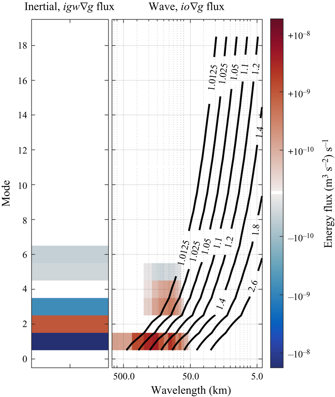
Having identified the two dominant physical mechanisms responsible for the nonlinear transfer of energy from inertial oscillations to internal gravity waves, we can now examine exactly which modes and scales are involved in the transfer. Figure 5 shows the nonlinear fluxes from only the two transfer mechanisms identified above, revealing the same dominant modes of transfer as in figure 3. Here, it is clear that the advection of geostrophic flow by internal gravity waves primarily drains energy from the $j=1$ inertial mode, but also shifts some energy to the $j=2$ mode. The advection of geostrophic flow by inertial oscillations transfers energy into the mode $j=1$ internal gravity waves at scale between 50 and 500 km. The results of figure 5 further imply that broader range of modes and scales seen to be exchanging energy in figure 3 must be explained by other mechanisms that transfer energy within the internal gravity wave modes. Indeed, at later times we find that internal gravity wave energy cascades to higher modes (not shown).

Figure 5. Same as figure 3, but showing only the two dominant mechanisms from figure 4. The wave panel shows flux from inertial oscillations advecting geostrophic motions and the inertial panel shows flux from internal gravity waves advecting geostrophic motions.

7. Modelling implications

In addition to the physical insights gained from applying the wave-vortex decomposition, there are also several implications for numerically modelling fluid flows. The first is the rather startling recognition that for the exponential stratification profile in figure 1, 257 evenly spaced vertical grid points in a pseudospectral model only resolves approximately 19 vertical modes. Conversely, this suggests that in cases of challenging stratification, modelling the equations of motion in wave-vortex space, as in appendix C, may actually be more computationally efficient than traditional spectral approaches.

One of the central claims of this manuscript is that the above wave-vortex decomposition can account for all variance of $(u,v,w,\rho )$ at any instant in time. In practice, however, ocean data and numerical models have a finite number of grid points, $N$, and it is not true in general that $N$ vertical modes will be resolved with $N$ grid points. As noted in Early et al. (Reference Early, Lelong and Smith2020), only if the grid points are at (or near) the Gaussian quadrature points of the vertical modes, $F(z)$ and $G(z)$, for all resolved $K$, will all variance project onto the modes. For the case of constant stratification, the Gaussian quadrature points are evenly spaced and the vertical modes coincide with cosine and sine bases. In this special case, the $N$ vertical grid points in the Boussinesq model will coincide with $N-2$ resolved internal modes, leaving only the Nyquist frequency unresolved plus a barotropic mode. However, as figure 1 demonstrates, for variable stratification, regions of rapidly changing stratification will lack resolution if an evenly spaced grid is used.

Because of the above issue, many numerical models use alternative vertical coordinates such as $\sigma$ (pressure) coordinates and density coordinates, or other more complicated hybrids, in order to better resolve the solutions. To resolve internal wave modes, Early et al. (Reference Early, Lelong and Smith2020) showed that a Wentzel–Kramers–Brillouin (WKB)-scaled coordinate more efficiently positions grid points than a density coordinate when capturing vertical modes. Once the vertical modes are computed, the Gauss quadrature points for the first $N$ modes can computed from the roots of the $N+1$th vertical mode. When creating a numerical model, these points are the optimal choice for resolving the vertical modes.

So what happens when grid points in a numerical model are not able to fully resolve the physics? From a diagnostic point of view, any variance not captured by the $M$ resolvable modes, results in a residual. The residual of projecting a function $f$ onto the $F$ modes is defined as $f_R \equiv f-\mathcal {F}^{-1}[ \mathcal {F}[f] ]$ where $\mathcal {F}$ projects using $M$ modes. For the Cyprus eddy example, the residual energy is shown in green in figure 2, and represents at most $0.3\,\%$ of the total energy, a $48\,\%$ increase from its initial value. Thus the initial conditions start with variance unresolved by the modal decomposition, and nonlinear processes further shift some of the resolved variance into unresolved variance over the course of the simulation. Because the evenly spaced $z$ grid in the model fully resolves the higher modes at lower depths, but only 19 modes near the surface, we expect an accumulation of residual energy at depth. Indeed, we find two peaks in residual energy between 450 and 500 m depth on day 37 of the simulation. How exactly this affects the resulting physics is not entirely clear. All we can say is that, given higher resolution, this residual energy would be associated with higher-mode internal waves which are presently not being represented correctly.

In the case of ocean observations with limited vertical sampling resolution, the issue is completely different than with a numerical model. In this case the physics is certainly evolving correctly, but the unresolved wave modes alias into the lower modes. Depending on the spectral slope of the unresolved modes, this aliasing may or may not have a significant impact on the coefficients of the resolved modes (Early et al. Reference Early, Lelong and Smith2020).

A second but related implication for modelling is that it may be advantageous to model the nonlinear equations of motions directly in wave-vortex space. This has the advantage of establishing which wave and vortex solutions are valid a priori, using the methods discussed above. Additionally, damping and/or small scale variance removal is then performed directly on the wave and vortex coefficients, which correspond to wave energy and potential enstrophy damping.

In light of the effective vertical resolution issues discussed above, the computational efficiency of modelling the equations of motion in wave-vortex space is relatively favourable for cases of nonlinear stratification. The rate limiting steps are the horizontal and vertical transformations required to compute the terms in (C18a). The two basic numerical operations to be performed on a vector of length $N$ are a matrix multiplication, which requires $2N^{2}$ operations, and a fast Fourier transformation (FFT), which requires $\frac {5}{2} \log _2 N - 3 N$ operations when transforming real variables (Canuto et al. Reference Canuto, Hussaini, Quarteroni and Zang2006). The vertical transformation must be computed as a matrix multiplication applied to each of the $N_x N_y/2$ wavenumber vectors of length $N_z$, for total computational cost of $N_z^{2} N_x N_y$. The horizontal transformation can be computed using an FFT algorithm applied to each depth $N_z$ for a total computational cost of $\frac {5}{2} N_z N_x N_y \log _2 N_x N_y - 3 N_z N_x N_y$. The transformation from wave-vortex space to physical space requires applying the vertical transformation 10 times (7 for the hydrostatic case) and the horizontal transformation 10 times. To finish the pseudospectral multiplication, the results must be projected back onto wave-vortex space for a grand total of 13 horizontal transformations and 10 vertical transformations. Assuming that $N_x = N_y$, the total computational cost of the horizontal and vertical transforms are approximately equal when $10 \log _2 N_x = N_z$, or $13 \log _2 N_x = N_z$ for the hydrostatic case. This means that for a horizontal resolution of $256^{2}$ the horizontal transformations dominate the computation time until approximately 80–100 vertical modes are used.