


1. Introduction
Buoyancy-driven flows in porous media arise in a number of important subsurface processes including subsurface storage of  ${\rm CO}_2$ in deep saline aquifers (Masson-Delmotte et al. Reference Masson-Delmotte, Zhai, Portner, Roberts, Skea and Shukla2021; Royal Society, Reference Royal Society2022), as well as the storage of hot, buoyant water for interseasonal aquifer thermal energy storage (Dudfield & Woods Reference Dudfield and Woods2014; Nielsen & Sørensen Reference Nielsen and Sørensen2016). Recently, there has also been a growing interest in the flow of hydrogen through aquifers for large-scale energy storage, where again buoyancy effects are key (Heinemann et al. Reference Heinemann2021).
Many models have been developed to describe buoyancy-driven flow through porous layers of uniform permeability, or permeability which slowly varies in space (Huppert & Woods Reference Huppert and Woods1995; Barenblatt Reference Barenblatt1996; Nordbotten & Celia Reference Nordbotten and Celia2006; Hinton & Woods Reference Hinton and Woods2018; Zheng & Stone Reference Zheng and Stone2022). However, many real geological strata are formed from the deposition of sediment, resulting in cross-bedded layers. The permeability in each of the layers is uniform and isotropic, but it changes from layer to layer, and so there is an effective macroscopic permeability on a scale larger than the thickness of the individual layers. This effective permeability is typically different along and across the bedding planes (Woods Reference Woods2015). Often the bedding planes are inclined to the boundaries of the formation (figure 1) and if the bedding planes are not parallel to the flow, then the pressure gradient and the flow direction are no longer aligned. With a pressure-driven flow, this can lead to shear developing in the flow as it migrates from one layer to another (Woods Reference Woods2015; Bhamidipati & Woods Reference Bhamidipati and Woods2020, Reference Bhamidipati and Woods2021). With a buoyancy-driven flow, the situation is somewhat different. First, if the bedding planes are horizontal and parallel to the boundary of the domain, then the long-time flow is controlled by the horizontal permeability, while the vertical permeability influences the time at which the flow transitions to this regime from the initial pressure-driven flow (Benham, Neufeld & Woods Reference Benham, Neufeld and Woods2022). However, when the bedding is inclined to the horizontal, the buoyancy-driven flow is influenced by both values of the permeability, and also the inclination of the boundary of the domain: here we show that, somewhat surprisingly, this can lead to currents of relatively buoyant fluid which run upslope either below the upper or above the lower boundary of the domain. Analysis of the controls on these flow patterns forms the subject of the present paper.

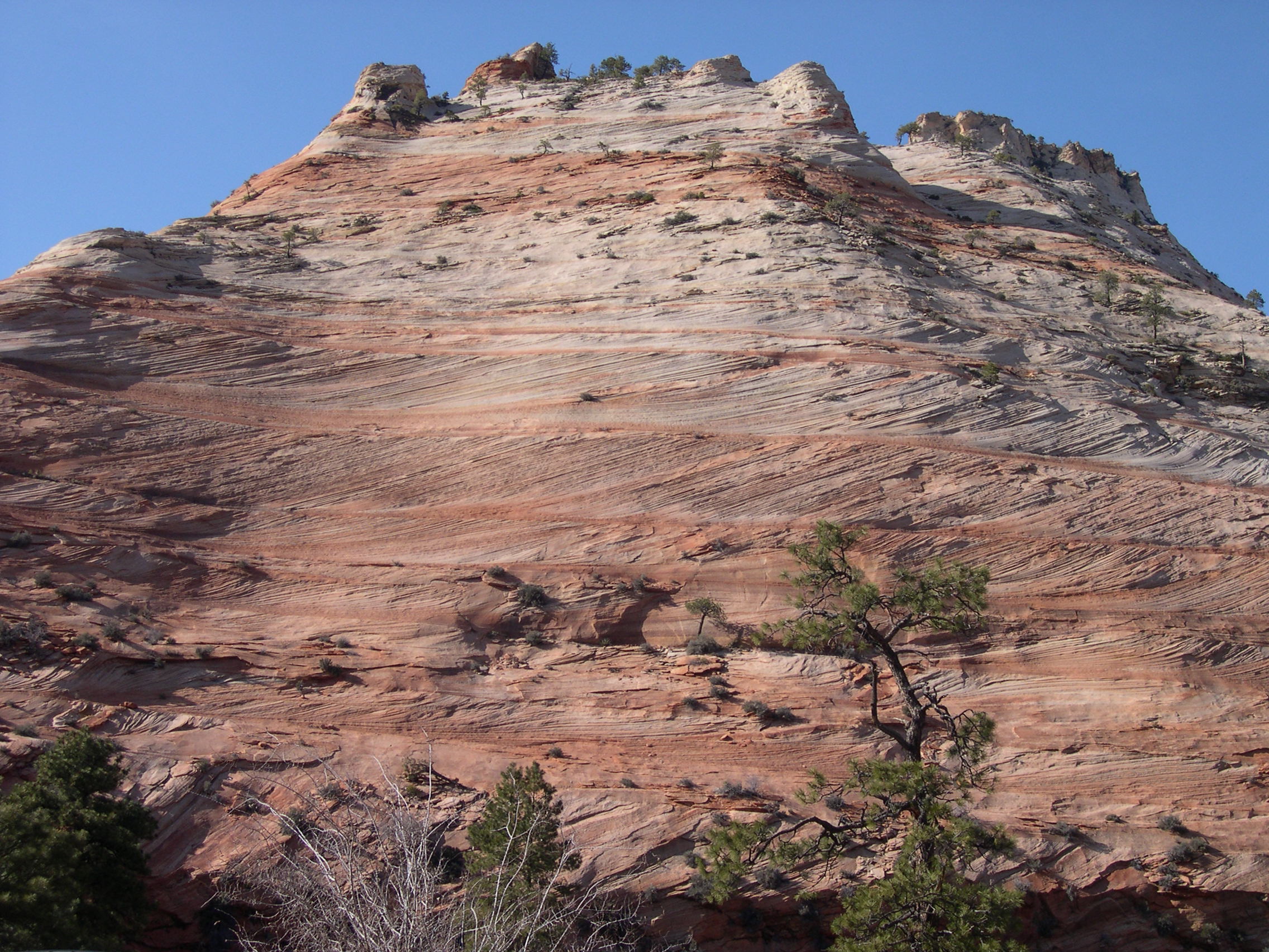
Figure 1. A photo of cross bedding taken at Zion National Park (Reif Reference Reif2008).
First, in § 2, we show that in a cross-bedded permeable layer, unconstrained buoyancy-driven flow rises at a finite angle to the horizontal, and we compare the predictions of a continuum model of the flow, based on the effective macroscopic permeability, with some new experiments. We then observe that in an inclined aquifer, the angle of inclination of the boundary of the aquifer to the horizontal relative to the inclination of this free buoyancy-driven flow determines whether the flow runs upslope below the upper or above the lower boundary of the layer. In § 3, we present a model to quantify the motion of such currents. The governing equation identifies two effective permeabilities, one controlling the upslope speed and one controlling the rate of spread of the current. In § 4, we present some new experiments of gravity-driven flow in an analogue experimental model of a cross-bedded layer, and test the validity of the model, showing that there is good agreement in both cases. In § 5, we consider the implications of our model.
The experiments presented in this paper concern a dense fluid flowing down an experimental cell and so in the remainder of the paper we consider the downward flow of a dense fluid although the analysis is mathematically identical to the case of a buoyant plume rising in an aquifer.
2. Gravity-driven free flow
We consider the flow of a dense fluid under gravity in a two-dimensional permeable layer of finite thickness which makes an angle  $\sigma$ to the horizontal (see figure 2). We let $k_1$ and $k_2$ be the effective permeability along and perpendicular to the bedding planes, respectively, where the angle $\theta$ is the direction of the high permeability bedding plane relative to the lower boundary of the aquifer (see figure 2). Darcy's law for the free, unconstrained buoyancy-driven flow along, $u$, and normal, $v$, to the boundary of the aquifer, averaged over a scale large relative to the scale of the layering, has the form (Bear Reference Bear1971)
 \begin{equation} {\boldsymbol{u}} =\begin{pmatrix} u \\ v \end{pmatrix} = \frac{\rho g}{\mu} \begin{pmatrix} \alpha & \beta \\ \beta & \gamma \end{pmatrix} \begin{pmatrix} \sin \sigma \\ - \cos \sigma \end{pmatrix} {,} \end{equation}
where  $\rho$ is the density, ${\mu}$ the viscosity of the fluid, $g$ the acceleration due to gravity, and the components of the permeability tensor are $\alpha = k_1 \cos ^2 \theta + k_2 \sin ^2 \theta$, $\beta = (k_1 - k_2) \cos \theta \sin \theta$ and $\gamma = k_2 \cos ^2 \theta + k_1 \sin ^2 \theta$.

Figure 2. Diagram summarising the flow structure for given aquifer inclination angles. The stripes in each picture represent the bedding planes on which sediment has been deposited. The image furthest to the left illustrates the coordinate system and parameters used in the model. The case  $\sigma = \sigma _c$ corresponds to the situation in which the flow is parallel to the boundary of the cell; $v$ denotes the component of the free-flow velocity in the direction of the $y$-axis, normal to the boundary.
We can define a free-flow angle  $\phi$ relative to the direction of the lower boundary of the aquifer using Darcy's law (2.1):
 \begin{equation} \tan( \phi ) = \frac{v}{u} = \frac{\beta \sin \sigma - \gamma \cos \sigma}{\alpha \sin \sigma - \beta \cos \sigma} {.} \end{equation}
 Equation (2.2) can be expressed in terms of  ${k_1}/{k_2}$:
 \begin{equation} \frac{k_1}{k_2} =- \cot( \sigma - \theta) \cot( \phi - \theta ) {.} \end{equation}
 In order to test this model, we have built a Hele-Shaw-type cell in which there are two perspex plates, each of size  $75 \times 30 \times 1 \ {\rm cm}$. The plates are separated by $1 \ {\rm mm}$ thick and $1 \ {\rm cm}$ wide strips along each of the four sides of the cell. There is a $1 \ {\rm cm}$ diameter injection port in the face of each corner of the cell through which the working fluid can be supplied. In one of the plates, we have milled a series of equispaced parallel channels of depth $2 \ {\rm mm}$, of width $3 \ {\rm mm}$ and separated by $5 \ {\rm mm}$. These channels make an angle $\theta = 20^{\circ }$ to the direction of the boundary of the cell and provide an analogue two-dimensional model of a cross-bedded rock (figure 3a) in which alternating layers of coarse and fine grains lead to alternating zones of high and low permeability and different effective permeabilities of the cell in the directions parallel to and normal to the bedding (Woods Reference Woods2015). We note that compared with real geological formations, the model is idealised in that we take the angle of the bedding planes and of the boundary of the flow cell to be constant, and we assume the permeability in the high- and low-permeability zones have the same value throughout the system. This simplified model enables us to identify some of the key controls on buoyancy-driven flow in such a cross-bedded layer.

Figure 3. (a) Schematic of the Hele-Shaw cell (not to scale). (b) Estimates of the permeability ratio  ${k_1}/{k_2}$ as a function of the aquifer inclination $\sigma$. The blue dots correspond to experimental measurements, and the red dashed line is the average of the data points. The data points $(\sigma, \phi )$ have values $(5, -125)$, $(25, -45 )$, $(36, -11)$, $(47,0)$, $(66,11)$, $(78,14)$ and $( 90, 16 )$. (c) Theoretical critical angle of inclination $\sigma _c$ as a function of the cross-bedding angle $\theta$ for three values of the permeability ratio ${k_1}/{k_2}$ (2, dotted green; 10, dashed blue; 100, solid red). (d) Photograph illustrating the free flow of fluid. Image is not to scale.
The experiments are recorded using a Nikon 5300 digital camera placed 2 m from the tank, which is backlit by a uniform light sheet (LightTape by Electro-LuminiX Lighting Corp.). The digital images are analysed using MatLab to measure the evolution of the shape and length of the current with time.
To test the model for the cross bedding, experiments were carried out for a range of angles of the boundary of the cell,  $\sigma$, and a glycerol–water mixture was pumped into the tank via an inlet port. In each case, we measured the angle of the free-flowing plume relative to the boundary of the cell, $\phi (\sigma )$ (see figure 3d). We then estimate the ratio of the permeability along and across the bedding plane using (2.3). In figure 3(b), we plot the estimate of the permeability ratio ${k_1}/{k_2}$ for a series of angles of inclination of the tank, $\sigma$, using the measured angles of the free flow, $\phi (\sigma )$. For the different values of $\sigma$, we obtain very similar estimates for ${k_1}/{k_2}$. The red dashed line in figure 3(b) shows the average value of our experimental estimate of ${k_1}/{k_2} = 5.6 \pm 0.3$. We note that this value implies that, for our experimental cell, the free flow is parallel to the actual boundary of the cell when $\sigma _c = 46 \pm 1^{\circ }$.
In figure 3(c), we illustrate the variation of the critical angle of the cell  $\sigma = \sigma _c$ for which $\phi = 0$ as a function of $\theta$. Curves are given for three values of ${k_1}/{k_2}$ according to (2.2). It is interesting to note that for ${k_1}/{k_2} \gg 1$, $\theta \approx \sigma _c$ or $\theta \approx 0$. The former case corresponds to the situation in which the direction of the bedding is nearly horizontal so that the gravitational force along the high-permeability direction $k_1$ is very small and, as a result, the component of gravity in the $k_2$ direction is sufficient to draw the flow along the direction of the boundary (see figure 2). In the other case, the bedding is nearly parallel to the boundary. In figure 3(d), we illustrate the free flow in a typical experiment.
3. Model
When the free flow is not parallel to the boundary of the formation, the fluid will flow along one of the boundaries. The pressure created by suppressing the flow normal to the boundary will result in the spreading of the fluid along the boundary, while the component of gravity along the boundary leads to a mean flow. We first consider the flow of a finite volume  $V$ with density $\rho$ and viscosity $\mu$ moving down the bottom boundary of the formation, inclined at an angle $\sigma$ in a cross-bedded porous medium with bedding planes at an angle $\theta$ to the boundary (see figure 2). We then consider the complementary case of a current which spreads along the top boundary. All the modelling considers two-dimensional flow, as would arise with injection from a horizontal line well aligned parallel to the bedding planes.
3.1. Flow along lower boundary
We let the current lie in the region  $0 < z < h(x,t)$ , $x_l< x < x_r$, where $x_l(t)$ and $x_r(t)$ represent the furthest extent of the current at its nose and tail, $h(x_l(t),t)=h(x_r(t),t)=0$. To model the flow, we first consider the vector velocity given by Darcy's law (Bear Reference Bear1971):
 \begin{equation} \boldsymbol{u} = \begin{pmatrix} u \\ v \end{pmatrix} =- \frac{1}{\mu} \begin{pmatrix} \alpha & \beta \\ \beta & \gamma \end{pmatrix} \begin{pmatrix} \dfrac{ \partial p }{ \partial x } - \rho g \sin \sigma \\[10pt] \dfrac{ \partial p }{ \partial z } + \rho g \cos \sigma \end{pmatrix} {,} \end{equation}
where  $p$ is the pressure, $\alpha, \beta$ and $\gamma$ are as in (2.1), and the permeability along and normal to the bedding planes are $k_1$ and $k_2$
$k_2$  $(k_2< k_1)$. Generally, in gravity-driven flows the fluid spreads out along the boundary and so eventually we expect $h\ll L = x_l-x_r$. At this point, the flow is dominantly parallel to the boundary (i.e. the $x$-direction) (Huppert & Woods Reference Huppert and Woods1995; Benham et al. Reference Benham, Neufeld and Woods2022), and our analysis considers this limit. We note that if the boundary is nearly vertical, the adjustment to this long and thin flow regime may require some time. Thus, we set $v = 0$ in (3.1) leading to the relation
 \begin{equation} \beta \frac{\partial p}{\partial x} + \gamma \frac{\partial p}{\partial z} =-\rho g ( \gamma \cos \sigma - \beta \sin \sigma). \end{equation}
This equation illustrates that the pressure follows the hydrostatic pressure along lines of slope  $\gamma / \beta$ to the boundary, and so it is convenient to introduce new coordinates (see figure 4a)
 \begin{equation} \eta = \gamma x - \beta z\quad\text{and}\quad \xi = \beta x + \gamma z {.} \end{equation}
In terms of these coordinates, (3.2) has the form
 \begin{equation} \frac{\partial p}{ \partial \xi} =- \frac{\rho g }{ \beta^2 + \gamma^2 } ( \gamma \cos \sigma - \beta \sin \sigma) {.} \end{equation}
This can be solved for fixed  $\eta$ noting that the pressure is zero on the free surface of the current, leading to the relation
 \begin{equation} p(\eta,\xi) =- \frac{\rho g (\xi - \xi_b) }{ \beta^2 + \gamma^2 } ( \gamma \cos \sigma - \beta \sin \sigma) {,} \end{equation}
where the point on the surface is  $(\eta,\xi _b(\eta ))$. Since the position of a point along the surface in the original coordinates is $(x,h(x,t))$, we have $\xi _b=\beta x+\gamma h(x)$ and $\eta = \gamma x - \beta h(x)$. It follows that
 \begin{equation} \xi_b \approx \frac{\beta} {\gamma} \eta +\left(\gamma +\frac{\beta^2} {\gamma}\right) h(\eta/\gamma) {,} \end{equation}
where we use the fact that the current is long and thin,  $x \gg h(x)$, to approximate $h(x)$. This leads to the revised expression
 \begin{equation} p = \frac{ \rho g }{ \beta^2 + \gamma^2 } \left(\frac{\beta \eta}{\gamma} - \xi \right) ( \gamma \cos \sigma - \beta \sin \sigma) + \frac{\rho g h}{\gamma} (\gamma \cos \sigma - \beta \sin \sigma) {.} \end{equation}
Using this expression for the pressure (3.7), we find the along-boundary horizontal component of the velocity  $u$ (3.1) in terms of $\xi$ and $\eta$:
 \begin{equation} u =- \frac{ \alpha
\gamma - \beta^2 }{\mu} \left[ \frac{ \rho g (\partial h/\partial \eta)}{\gamma}(\gamma \cos \sigma - \beta \sin \sigma) -
\left( \frac{ \alpha \gamma - \beta^2 }{\gamma} \right)
\rho g \sin \sigma \right] {.}
\end{equation}
\begin{equation} u =- \frac{ \alpha
\gamma - \beta^2 }{\mu} \left[ \frac{ \rho g (\partial h/\partial \eta)}{\gamma}(\gamma \cos \sigma - \beta \sin \sigma) -
\left( \frac{ \alpha \gamma - \beta^2 }{\gamma} \right)
\rho g \sin \sigma \right] {.}
\end{equation}
We can transform (3.8) into the original coordinates, to track the flow along the boundary, noting that, on the  $x$-axis, ${\partial h}/{\partial \eta } = ({1}/{\gamma })({\partial h}/{\partial x})+O(h^2)$ This leads to the approximate equation
 \begin{equation} u =- \frac{ \rho g}{\mu} [ ( k_{{p}} \cos \sigma - k_{{n}} \sin \sigma) (\partial h/\partial \eta) - k_{{p}} \sin \sigma] {,} \end{equation}
where
 \begin{equation} k_p = \frac{\alpha \gamma - \beta^2}{\gamma} \quad\text{and}\quad k_n = \frac{(\alpha \gamma - \beta^2) \beta }{\gamma^2} {.} \end{equation}
We now combine (3.9) with the local conservation of mass averaged over a scale larger than the width of the cross beds
 \begin{equation} \frac{\partial h}{\partial t} =- \frac{ \partial (h u)}{\partial x} {,} \end{equation}
leading to the governing equation
 \begin{equation} \frac{\partial h}{\partial t} = \frac{\rho g}{\mu} \frac{\partial }{\partial x} [ ( k_{p} \cos \sigma - k_{n} \sin \sigma) h (\partial h/\partial x) - k_{p} \sin \sigma h] {,} \end{equation}
where
 \begin{equation} k_p = \frac{k_1 k_2}{k_1 \sin^2 \theta + k_2 \cos^2 \theta} \quad\text{and}\quad k_n = \frac{ k_1 k_2 (k_1 - k_2) \sin 2 \theta }{2(k_1 \sin^2 \theta + k_2 \cos^2 \theta )^2} {.} \end{equation}
Note that  $k_p$ corresponds to the effective permeability for the along-boundary flow, and matches the value for pressure-driven flow (Woods Reference Woods2015). The term $k_p \cos \sigma - k_n \sin \sigma$ represents the effective permeability associated with the buoyancy force normal to the slope and this drives the diffusive spreading of the current. In the case that this term is zero, the flow is predicted to move parallel to the boundary (2.3). If this term is negative, then the equation would involve a negative diffusivity: mathematically the equation would then suggest a localisation and deepening of the flow rather than the diffusive spreading of the flow, but physically this corresponds to the case in which the free flow is directed to the opposite boundary of the cell. As a result, the flow migrates across the cell and then spreads along the other boundary of the system. Note that when dealing with a uniform porous medium ( $k = k_1 = k_2$), $k_p = k$ and $k_n = 0$, (3.12) reduces to the classical porous medium equation (Huppert & Woods Reference Huppert and Woods1995).

Figure 4. (a) The coordinates used in the derivation of the model for the flow along the bottom boundary. (b) Coordinate system used to describe flow on the top boundary.
The problem is closed by imposing volume conservation:
 \begin{equation} \int_{x_l}^{x_r} h \,{{\rm d}x} = V, \end{equation}
where V is the volume per unit width.
3.2. Flow along upper boundary
In the case in which the current spreads down slope along the upper boundary, we introduce coordinates defined relative to the top of the aquifer (see figure 4b). We follow a similar analysis to that in § 3.1 to derive the governing equation
 \begin{equation} \frac{\partial h}{\partial t} = \frac{\rho g}{\mu} \frac{\partial }{\partial x} [ ( k_n \sin \sigma - k_p \cos \sigma ) h (\partial h/\partial x) + k_p \sin \sigma h] {,} \end{equation}
In this case, the coefficient of the diffusive spreading term is of equal magnitude but opposite sign. This ensures that for all angles, as the current spreads out along the appropriate boundary, the diffusivity is positive. Note also that  $x$ is now directed upslope and this leads to a change in the sign of the advection term.
4. Experimental tests of the model
4.1. Flow along a horizontal boundary
We have carried out three experiments in which the cell is horizontal and a finite volume of fluid per unit width of the cell (experiment 1,  $85\ {\rm cm}^2$; experiment 2, $117\ {\rm cm}^2$; experiment 3, $96\ {\rm cm}^2$) was released at the end of the cell. A glycerol–water solution in the mass ratio of 4 : 1 was used as the working fluid, and the density and viscosity of the solution was estimated as a function of the temperature of the mixture (Cheng Reference Cheng2008). The bedding angle was directed at $20^\circ$ (experiments 1 and 2) and $160^\circ$ (experiment 3) to the direction of flow. For these experiments, we expect the governing equation (3.12) to take the form
 \begin{equation} \frac{\partial h}{\partial t} = \frac{ k_{p} \rho g}{\mu} \frac{\partial }{\partial x} [ h (\partial h/\partial x) ] {,} \end{equation}
which is the classical porous medium equation with permeability  $k_p$. Equation (4.1) admits a similarity solution of the form (Huppert & Woods Reference Huppert and Woods1995)
 \begin{align} h = \left( \frac{ k_p \rho g t}{ \mu V^2} \right)^{- {1}/{3}} f(\eta_s) ,\quad \text{where } \eta_s = \frac{x}{ \left( \dfrac{V k_p \rho g t}{\mu} \right)^{{1}/{3}}} \quad{\rm{and}}\quad f(\eta_s)= \frac{1}{6} ( {\eta_0}^2 -\eta_s^2), \end{align}
where  $\eta_{0}$ is the point at which $f(\eta_{0})=0$, and is specific using volume conservation (per unit width). At a series of times during each experiment, we measure the shape of the current and rescale the length and height of the current according to the classical solution, using an estimate for $k_p$. We find that after an initial transient, the scaled current shape converges. At each time, we calculate the fractional area difference between the model and the instantaneous shape as given by
 \begin{equation} \text{fractional area difference } = \sqrt{ \int_0^{\eta_{{end} } } \,{\rm d} \eta \left( f(\eta_s) - f_e(\eta_s) \right)^2 } {,} \end{equation}
with  $f_e$ the scaled depth of the experimental current. The leading edge of the current, $\eta _{{end}}$, is taken as the larger of the leading edges of the experimental current and the model current. Note that we define $f(\eta ) =0$ for $\eta > \eta _0$.
We systematically vary  $k_p$ to find the value with the minimum average fractional area difference across the three experiments (figure 5a). The somewhat irregular nature of the interface, caused by the alternating thickness of the channels and the associated difference in the capillary imbibition height, which is approximately 2–4 mm, leads to some discrepancy between the model and experimental interface shape, but the overall dynamics is controlled by the gradient of the buoyancy head, as described by (3.12). Allowing for an averaged fractional error within $5\,\%$ of the minimum, we estimate $k_p = 1.21 \pm 0.06 \times 10^{-7}\ {\rm m}^2$. Using this range for $k_p$ along with the permeability ratio ${k_1}/{k_2}$ as estimated in § 2, we estimate that $k_n = 1.17 \pm 0.05 \times 10^{-7}\ {\rm m}^2$.

Figure 5. (a) The average fractional area difference calculated by comparing the scaled shape of three experimental currents, each measured at three times, with the model prediction, as a function of varying  $k_p$. The volume of the three currents were $85$,
$85$,  $117$ and $96\ {\rm cm}^2$. (b) The self-similar depth of the currents $f$ as a function of $\eta _s$. In these calculations, the best-fit estimate of $k_p$ is used in the scaling of the experimental data. Each profile was measured at time $t = 80$ s. Experiments 1 and 2, as seen in the legend of the figure have cross-bedding angle $\theta =20^\circ$, while experiment 3 has bedding angle $\theta = 160^\circ$. (c,d) Photographs of horizontal gravity currents at $t=80$ s with bedding angles (c) $\theta = 20^{\circ }$ (experiment 1) and (d) $\theta = 160^\circ$ (experiment 3).
In figure 5(b) we compare the scaled depth of the current,  $f(\eta _s)$ as a function of $\eta _s$, for the similarity solution and each of the experimental currents, as measured at $t=80$ s. This illustrates the good correspondence between the model and experiment.
It is interesting to note that the model predicts that, for a horizontal flow, the motion is identical when the direction of the cross bedding is reversed (i.e.  $\theta \rightarrow 180^\circ -\theta$); in figure 5(c,d) we present photographs from two experiments of horizontal gravity currents, one with $\theta = 20^\circ$ and the other with $\theta = 160^\circ$, illustrating this correspondence.
4.2. Inclined flows
Given the agreement of the model with the free-flow experiments and the experiments with a horizontal boundary, we now test the model for flows which migrate downslope, either above the lower boundary or below the upper boundary of the channel (cf. figure 2). This also provides a test for our experimental estimates of the permeabilities  $k_p$ and $k_n$.
A series of experiments were carried out in which a finite volume of fluid was released in the cell at a series of different inclinations. Two example experiments are shown in figures 6(a) and 6(b) corresponding to currents moving downslope above the lower and below the upper boundary, with  $\sigma = 27^{\circ }$ and $79^{\circ }$, respectively. The experiment with the larger angle illustrates the novel feature of a current moving downslope below the upper boundary in a cross-bedded domain. The similarity solution in these cases is of the form
 \begin{equation} \left.\begin{gathered} h = \left( \frac{ \rho g (-1)^{j}( k_p \cos \sigma - k_n \sin \sigma) t}{ \mu V^2} \right)^{- {1}/{3}} f(\eta_s), \\ \eta_s = \frac{x - x_{{cm} }(t)}{ \left( \dfrac{V \rho g (-1)^{j}( k_p \cos \sigma - k_n \sin \sigma ) t}{\mu} \right)^{{1}/{3}}}, \end{gathered}\right\} \end{equation}
where the subscript  $j= 0$ represents flow along the bottom boundary and $j=1$ the flow below the top boundary. In each case, the centre of mass $x_{cm}$, is defined as
 \begin{equation} x_{{cm}}(t) = \left.\int_{x_l}^{x_r} x h \,{{\rm d}x} \right/ \int_{x_l}^{x_r} h\, {{\rm d} x} {.} \end{equation}
We measured the shape of the experimental currents, and rescaled the height  $h$ relative to the experimental centre of mass $x_{{cm}}$ to compare the spreading of the fluid with the theoretical prediction, using the best fit values of $k_p$ and $k_n$ found in the previous section. The rescaled current shape is shown at a series of times, as the flow spreads out over the length of the experimental tank, and compared with the model solution in figure 6(c,d). It is seen that the scaled experimental current shape is in good accord with the model. However, as the current moves down the slope, a small amount of fluid becomes capillary trapped in the channel boundaries once the tail of the flow begins to move downslope. This leads to a gradual loss of mass. In figure 7, we have plotted the fractional area error for both the bottom (a) and top (b) cases as a function of time. The error at first decreases to 7 %–9 %, as the flow converges towards the finite-mass similarity solution. However, we note that at later times, as more fluid is lost by capillarity at the tail of the flow, the mismatch in the fractional area error gradually begins to increase.

Figure 6. (a) Photograph of a current moving downslope above the bottom boundary. (b) Photograph of a current moving downslope below the upper boundary. (c,d) Similarity height  $f$ plotted as a function of the similarity distance $\eta _s$, for a current of finite volume at times $t = 10\ {\rm s}$, $20\ {\rm s}$ and $30\ {\rm s}$ after release moving along the base of the tank (c), and $t = 4\ {\rm s}$, $8\ {\rm s}$ and 12 s for a current moving downwards below the upper boundary of the tank (d). The angles of inclination of the cell are $\sigma = 27^{\circ }$ and $\sigma = 79^{\circ }$ respectively.

Figure 7. Fractional area difference as a function of varying time for the bottom (a) and top (b) cases.
5. Conclusion
We have investigated gravity-driven flows in a cross-bedded inclined porous formation. In § 2, we demonstrated that owing to the cross bedding, the free gravity-driven flow is inclined to the vertical. As a result, depending on the inclination of the aquifer to this free-flow angle, a gravity-driven flow may migrate down the upper or lower boundary of a finite-thickness layer. In § 3, we developed a model for the flow showing that the cross-slope component of gravity leads to diffusive spreading, irrespective of whether the flow spreads on the upper or lower boundary. In § 4, we presented some experiments using a model of a two-dimensional cross-bedded formation and we showed that the simple analogue experimental gravity currents evolve in accord with our model predictions. The experiments illustrate that, with cross bedding, currents may spread along the upper or lower boundary of the domain depending on the angle of the bedding and the boundary of the domain, in accord with the regime diagram (figure 2).
In sedimentary formations, grain size can vary by around two orders of magnitude (Sun et al. Reference Sun, Bloemendal, Rea, Vandenberghe, Jiang, An and Su2002) and the associated permeability could potentially vary by up to four orders of magnitude (Bear Reference Bear1971). This suggests that the ratio  ${k_1}/{k_2}$ may take on a wide range of values. For aquifer inclinations greater than the solid lines in figure 3(c), each of which corresponds to a given permeability ratio, a plume of buoyant fluid would preferentially rise along the lower rather than upper boundary of the aquifer. It is seen that as the permeability ratio increases, the chance that a buoyant current runs upslope above the lower boundary of the aquifer increases.
Knowledge of the expected location of a plume of buoyant fluid is important in a range of applications. For example, in  $\textrm {CO}_2$ storage, in cases in which the $\textrm {CO}_2$ migration is dominated by buoyancy rather than capillary forces, differences in the location of the plume as it rises through the formation owing to cross bedding may result in different distributions of the capillary trapped $\textrm {CO}_2$ following injection (Hesse, Orr & Tchelepi Reference Hesse, Orr and Tchelepi2008) (e.g. figure 8). Also, if a pool of $\textrm {CO}_2$ collects at the top of an anticline, it may then dissolve into the underlying formation water, producing a plume of $\textrm {CO}_2$-saturated and hence dense water. This may flow downdip into a region of unsaturated water, but depending on the geometry of any cross bedding, the flow could run downdip below the upper boundary of the formation, rather than along the lower boundary. Observation wells, designed to monitor the dissolution, might then detect $\textrm {CO}_2$ saturated water in the upper part of the aquifer, far downdip from the main $\textrm {CO}_2$ plume, while conventional models would suggest it should be at the base of the aquifer (Woods & Espie Reference Woods and Espie2012). In aquifer thermal energy storage, hot and buoyant fluid is injected and subsequently extracted from the formation. If the system is cross-bedded, the plume of hot water and hence thermal energy may run updip along the lower boundary of the formation rather than below the upper boundary and this can impact how much of the thermal energy can be recovered (Dudfield & Woods Reference Dudfield and Woods2014). We plan to explore these effects in more detail, and to extend the analysis to include three-dimensional effects in further work.

Figure 8. Diagram illustrating a possible pattern for the migration of a plume of buoyant injectate (green fluid) in a cross-bedded anticline initially saturated with saline aqueous solution (blue fluid), in the case that the buoyancy forces dominate the flow of the injectate. If the flow of  $\textrm {CO}_2$ is buoyancy dominated, this figure identifies that different patterns of ascent and of capillary trapping may arise depending on the bedding.
Declaration of interests
The authors report no conflict of interest.


 Open access