


1. Introduction
The present manuscript investigates how surface water waves impact temperature transport at the seabed. The subject of temperature conduction in fluids is incredibly varied, with a vast literature (see e.g. Landau & Lifshitz (Reference Landau and Lifshitz1989) and White (Reference White1991) for useful background information). In the most general setting, the temperature distribution and flow field mutually influence one another, which makes for a rich and complex problem. However, it is often possible to adopt the simplifying assumption that the flow is independent of temperature.
When it comes to the oceanic environment, temperature transport has been studied at large as well as small scales. At the largest scales, wind-driven gyres and overturning circulation are responsible for oceanic heat transport from the tropics to higher latitudes (Ferrari & Ferreira Reference Ferrari and Ferreira2011). Turning to the small scales, research investigations have been devoted to studying temperature in the surface boundary layer, which forms the interface between ocean and atmosphere. Early work by O'Brien (Reference O'Brien1967) considered heat transfer at wavy surfaces specified in Lagrangian coordinates, whereas Witting (Reference Witting1971) later investigated the role of surface gravity and capillary waves on surface heat flux. Experimental work by Veron, Melville & Lenain (Reference Veron, Melville and Lenain2008) has also underscored the importance of surface gravity waves in driving air–sea heat transfer in the ocean.
To the best of our knowledge, the effect of surface waves on heat transfer in the seabed boundary layer has not hitherto been studied. Whereas the motion associated with surface waves decreases with depth, in intermediate depths (relative to the length scale of the waves) this motion extends all the way down the water column. This is an important driver of seabed mass transport (Mei & Chian Reference Mei and Chian1994), as well as the transport of solutes and contaminants (Winckler, Liu & Mei Reference Winckler, Liu and Mei2013). In the present paper, we show that this motion is responsible for temperature convection.
For a suitable choice of scales, and an idealised flat and smooth bed, we are able to treat the problem analytically by means of perturbation theory. We assume the fluid is incompressible and viscous, enabling the fluid density to be independent of fluid pressure, and the hydrodynamic problem to be decoupled from its thermodynamic counterpart. The second-order wave-induced motion is determined by an approach analogous to that used in investigating mass transport by Mei, Stiassnie & Yue (Reference Mei, Stiassnie and Yue2005, Chapter 10). This motion drives flow in the boundary layer, and results in a convection–diffusion equation for the temperature. This approach is mathematically similar to earlier studies by Lighthill (Reference Lighthill1950, Reference Lighthill1954).
By introducing a slow time scale and similarity variables, we are able to solve the equation for the seabed temperature transport to yield explicit expressions for the heat transfer. We also obtain a theoretical criterion by which to estimate the frequency of free-surface waves that maximises heat exchange, and validate the analytical approximation by comparison with a full numerical solution based on a finite-difference scheme. Our results suggest that the effect of free-surface waves should be included in existing models to ensure proper estimation of the temperature field near the seabed, especially when such models are applied in practice.
2. Mathematical model
Let us consider a two-dimensional fluid domain  $\varOmega (x,z,t)$, where
  $x$ is horizontal distance,
  $z$ is vertical distance upwards from the horizontal seabed and
  $t$ is time. We assume that the fluid is viscous and incompressible, in which case the equation of heat convection and diffusion in a laminar boundary layer assumes the simplified form (Landau & Lifshitz Reference Landau and Lifshitz1989)
 \begin{equation} \frac{\partial T}{\partial t}+u\frac{\partial T}{\partial x}+w \frac{\partial T}{\partial z}=\chi \nabla^2T, \end{equation}
where  $T$ is temperature,
  $\chi$ is thermometric conductivity and
  $(u,w)$ are the horizontal and vertical components of the velocity field. Diffusion effects are expected to be greatest close to a heat source because of the low thermometric conductivity of water. For this reason, we introduce the following non-dimensional quantities (Mei et al. Reference Mei, Stiassnie and Yue2005; Michele & Renzi Reference Michele and Renzi2019; Michele, Renzi & Sammarco Reference Michele, Renzi and Sammarco2019):
 \begin{equation} x'=x k,\quad z'=z/\delta,\quad u'=u/(A\omega),\quad w'=w/(A\omega k\delta),\quad t'=\omega t,\quad T'=T/T_b, \end{equation}
where  $k$ is a typical wavenumber of the propagating surface waves,
  $\omega$ the frequency of wave oscillations,
  $A$ the amplitude of oscillations near a seabed of intermediate depth
  $h$,
$h$,  $T_b$ is the temperature of the seabed,
  $\delta =\sqrt {2\nu /\omega }$ the scale of the boundary-layer thickness and
  $\nu$ the kinematic viscosity coefficient. We also define the small parameter
  $\epsilon =A k\ll 1,$ which represents the steepness of the propagating waves. Substitution of (2.2a–f) into (2.1) yields the governing equation in non-dimensional form:
 \begin{equation} \frac{\partial T'}{\partial t'}+\epsilon\left(u'\frac{\partial T'}{\partial x'}+w' \frac{\partial T'}{\partial z'}\right)=\mu^2\left(\frac{\partial^2 T'}{\partial x'^2}\delta^2k^2+ \frac{\partial^2 T'}{\partial z'^2}\right),\end{equation}
where the small parameter  $\mu$ is defined by
 \begin{equation} \mu=\sqrt{\frac{\chi}{\omega\delta^2}}=\sqrt{\frac{\chi}{2\nu}},\quad \mu\sim \textit{O}\left(\epsilon\right). \end{equation}
The assumption that  $\mu$ is comparable with
  $\epsilon$ is justified for fluids characterised by small thermometric conductivity, such as water, as will be shown in § 3.
Given that  $\delta k\sim \textit {O}(\epsilon ^4)$ is very small, (2.3) can be simplified as follows:
 \begin{equation} \frac{\partial T'}{\partial t'}+\epsilon\left(u'\frac{\partial T'}{\partial x'}+w' \frac{\partial T'}{\partial z'}\right)=\mu^2\frac{\partial^2 T'}{\partial z'^2}+ \textit{O}(\epsilon^3),\end{equation}
in which we neglect third-order contributions. Therefore, convective effects driven by the moving fluid appear at second order  $\textit {O}(\epsilon )$, whereas diffusion is significant at third order
  $\textit {O}(\epsilon ^2)$. Having obtained the governing equation for fluid temperature, we now derive expressions for the components of the fluid velocity field in the boundary layer at the seabed. The dynamic problem is decoupled from its thermodynamic counterpart, and so the water-particle velocity components
  $(u,w)$ are determined by analogy to the analysis of mass-transfer phenomena by Mei et al. (Reference Mei, Stiassnie and Yue2005, chap. 10).
2.1. Flow field in the laminar boundary layer
The mass continuity and Navier–Stokes equations in the boundary-layer region can be approximated by
 $$\begin{gather} \frac{\partial u}{\partial x}+\frac{\partial w}{\partial z}=0, \end{gather}$$
 $$\begin{gather}\frac{\partial u}{\partial t}+u\frac{\partial u}{\partial x}+w\frac{\partial u}{\partial z}={-}\frac{1}{\rho}\frac{\partial P}{\partial x}+\nu \frac{\partial^2 u}{\partial z^2}, \quad \frac{1}{\rho}\frac{\partial P}{\partial z}+g=0, \end{gather}$$
where  $\rho$ denotes fluid density,
  $g$ acceleration due to gravity and
  $P$ the total pressure. Here, the dynamic component of the pressure
  $p=P-\rho g z$ does not depend on vertical elevation and matches the value in the inviscid flow region outside the boundary layer. Hence,
 \begin{equation} \frac{\partial u}{\partial t}+u\frac{\partial u}{\partial x}+w\frac{\partial u}{\partial z}= \frac{\partial U}{\partial t}+U\frac{\partial U}{\partial x}+\nu \frac{\partial^2 u}{\partial z^2}, \end{equation}
where  $U$ is the horizontal component of the inviscid flow velocity at the seabed, and the corresponding vertical component is zero. By assuming the following perturbation expansion in terms of
  $\epsilon =A k\ll 1$,
 \begin{equation} u=u_1+u_2+O(\omega A\epsilon^2), \end{equation}
with  $u_1=O(\omega A)$,
  $u_2=O(\omega A \epsilon )$, we obtain the following leading-order problem
  $O(1)$:
 $$\begin{gather} \frac{\partial u_1}{\partial t}=\frac{\partial U}{\partial t}+\nu \frac{\partial^2 u_1}{\partial z^2}, \end{gather}$$
 $$\begin{gather}u_1=0,\quad z=0, \end{gather}$$
 $$\begin{gather}u_1=U,\quad z\gg\delta. \end{gather}$$
Given that
 \begin{equation} U=\text{Re}\{U_0 \,\textrm{e}^{-\mathrm{i}\omega t}\}, \end{equation}
with  $U_0$ a function of
  $x$, we obtain
 \begin{equation} u_1=\text{Re}\{U_0 (1-\textrm{e}^{-\left(1-\mathrm{i}\right)z'}) \textrm{e}^{-\mathrm{i}\omega t}\}. \end{equation}
By integrating the continuity equation (2.6), the vertical component of water-particle velocity at the leading order may be expressed as
 \begin{equation} w_1=\text{Re}\left\{\delta \frac{\partial U_0}{\partial x} \left[\frac{1+\mathrm{i}}{2}\left(1-\textrm{e}^{{-}z'(1-\mathrm{i})}\right)-z'\right] \textrm{e}^{-\mathrm{i}\omega t}\right\}. \end{equation}
The governing equation at second order is given by
 \begin{equation} \frac{\partial u_2}{\partial t}-\nu \frac{\partial^2 u_2}{\partial z^2}=U \frac{\partial U}{\partial x}-\left(u_1\frac{\partial u_1}{\partial x}+w_1 \frac{\partial u_1}{\partial z}\right), \end{equation}
which admits second (2 $\omega$) and zeroth harmonic solutions. The second-harmonic component contributes only a small oscillatory correction to the first harmonic obtained at leading order, which can be eliminated by time averaging over the period
  $2{\rm \pi} /\omega$. More significant is the drift associated with the zeroth harmonic, for which we obtain
 \begin{equation} -\nu\frac{\partial^2\overline{u_2}}{\partial z^2}=\overline{U\frac{\partial U}{\partial x}}- \left(\frac{\partial\overline{u_1^2}}{\partial x}+\frac{\partial \overline{u_1w_1}}{\partial z}\right), \end{equation}
where the overbar represents the averaged value of the relevant variables. The boundary conditions at second order reduce to
 $$\begin{gather} \overline{u_2}=0,\quad z=0, \end{gather}$$
 $$\begin{gather}\frac{\partial \overline{u_2}}{\partial z}=0,\quad z\gg\delta, \end{gather}$$
and the horizontal drift velocity component is given by
 \begin{equation} \overline{u_2}={-}\frac{1}{\omega}\text{Re}\left\{F_1U_0\frac{\partial U_0^*}{\partial x}\right\}, \end{equation}
in which
 \begin{equation} F_1=\frac{1+\mathrm{i}}{4}\{{-}3\mathrm{i}+\textrm{e}^{{-}2z'} [{-}1-(1+\mathrm{i})\textrm{e}^{z'(1-\mathrm{i})}+ 2\,\textrm{e}^{z'(\mathrm{i}+1)}(z'+2\mathrm{i}+1)]\}, \end{equation}
and  $()^*$ denotes the complex conjugate of the relevant variable. Let us consider a progressive wave propagating in the positive direction described by the following velocity potential (Mei et al. Reference Mei, Stiassnie and Yue2005, Chapter 1):
 \begin{equation} \varPhi=\text{Re}\left\{\frac{-\mathrm{i} A g}{\omega} \frac{\cosh{k z}}{\cosh{k h}}\exp({\mathrm{i}\left(kx-\omega t\right)})\right\},\quad \omega^2=gk\tanh(kh), \end{equation}
in which  $A$ is the wave amplitude and
  $h$ is the undisturbed water depth. The inviscid horizontal water-particle velocity component at
  $z=0$ is thence given by
 \begin{equation} \left.\varPhi_x\right|_{z=0}=U=\text{Re}\left\{\frac{A \omega}{\sinh{k h}} \exp({\mathrm{i}\left(kx-\omega t\right)})\right\}\rightarrow U_0=\frac{A \omega}{ \sinh{k h}}\textrm{e}^{\mathrm{i}kx}. \end{equation}
Substitution of (2.23) into expressions (2.14), (2.15) and (2.20) yields the following horizontal and vertical water-particle velocity components in the boundary layer:
 \begin{align} u&=\frac{A\omega}{\sinh{k h}}\left\{ \text{Re} \left\{\left(1-\textrm{e}^{-\left(1-\mathrm{i}\right)z'}\right)\exp({\mathrm{i} \left(kx-\omega t\right)})\right\}\right.\nonumber\\ &\quad \left.+\frac{A k\,\textrm{e}^{{-}z'}}{2\sinh{k h}}\left[-\left(2+z'\right) \cos z'+2\cosh z'+(1-z')\sin z'+\sinh z'\right]\right\}, \end{align}
 \begin{align} w&=\frac{A\omega k\delta}{\sinh{kh}} \text{Re}\left\{\mathrm{i}\exp({\mathrm{i}\left(kx-\omega t\right)}) \left[\frac{1+\mathrm{i}}{2}\left(1-\textrm{e}^{{-}z'\left(1-\mathrm{i}\right)}\right)-z'\right]\right\}. \end{align}
These expressions are used in the next section to solve the temperature distribution in the boundary-layer region.
2.2. Convection and diffusion of temperature in the boundary layer
We introduce the following expansion for the temperature  $T'$:
$T'$:
 \begin{equation} T'=T_1'\left(x',z',t',\tau'\right)+\epsilon T_2'\left(x',z',t',\tau'\right)+ \epsilon^2T_3'\left(x',z',t',\tau'\right),\end{equation}
where  $\tau '=\epsilon ^2t'$ denotes the slow time scale of diffusion effects. Substitution of (2.26) in (2.5) yields a sequence of boundary-value problems at different orders. The leading-order problem yields
 \begin{equation} \frac{\partial T_1'}{\partial t'}=0, \end{equation}
indicating that the temperature at  $\textit {O}(1)$ is a function of spatial coordinates and slow time scale only, i.e.
  $T_1'(x',z',\tau ')$. The governing equation at second order
  $\textit {O}(\epsilon )$ expressed in physical variables is given by
 \begin{equation} \epsilon\frac{\partial T_2}{\partial t}+u_1\frac{\partial T_1}{\partial x}+w_1 \frac{\partial T_1}{\partial z}=0, \end{equation}
representing the convective effect of the oscillatory flow, where the terms  $(u_1,w_1)$ are given by (2.14)–(2.15). Note that the term
  $\epsilon$ reappears here because of our use of physical variables. The water-particle velocity components are harmonic in time, and so the response
  $T_2$ can be written as
 \begin{align} T_2 &={-}\frac{1}{\epsilon\omega}\text{Re}\left\{\mathrm{i}\,\textrm{e}^{-\mathrm{i}\omega t} \left\{\frac{\partial T_1}{\partial x} U_0 \left(1-\textrm{e}^{-\left(1-\mathrm{i}\right)z'}\right) \right.\right. \nonumber\\ &\quad \left.\left.+\,\delta\frac{\partial T_1}{\partial z}\frac{\partial U_0}{\partial x}\left[\frac{1+\mathrm{i}}{2} \left(1-\textrm{e}^{{-}z'\left(1-\mathrm{i}\right)}\right)-z'\right]\right\}\right\}, \end{align}
in which  $U_0$ is given by (2.23). Hence, the component
  $T_2$ oscillates periodically in time with the frequency of the propagating waves
  $\omega$. Note that the corresponding slowly varying amplitude
  $T_1$ is an unknown yet to be determined. Moving to third order
  $\textit {O}(\epsilon ^2)$, we obtain the following non-dimensional governing equation:
 \begin{equation} \frac{\partial T_3'}{\partial t'}+\frac{\partial T_1'}{\partial \tau'}+u_1' \frac{\partial T_2'}{\partial x'}+w_1'\frac{\partial T_2'}{\partial z'}+u_2' \frac{\partial T_1'}{\partial x'}=\frac{\mu^2}{\epsilon^2}\frac{\partial^2 T_1'}{\partial z'^2}.\end{equation}
Averaging over a wave period yields an equation for the slow evolution of the leading-order temperature  $T_1$ which, in physical variables, takes the simplified form
 \begin{equation} \frac{\partial T_1}{\partial t}+\tilde{u}\frac{\partial T_1}{\partial x}-\chi \frac{\partial^2 T_1}{\partial z^2}=0, \end{equation}
where the velocity  $\tilde {u}$ in the convective term reads
 \begin{equation} \tilde{u}=\frac{A^2\omega k}{2\sinh^2{kh}}\textrm{e}^{{-}z'}\left(4\cosh {z'}+\sinh{z'}-4\cos{z'}\right). \end{equation}
Expression (2.31) with forcing term (2.32) governs the spatial and temporal evolution of temperature at leading-order  $T_1$. Governing equation (2.31) suggests that convection effects occur horizontally, whereas temperature diffusion occurs normal to the seabed. In the following, it is convenient to work with a relative temperature
  $T_R(x,z,t)=T_1(x,z,t)-T_w,$ where
  $T_w$ is the ambient water temperature at a large distance from the seabed. We then consider the steady-state configuration
  $\partial T_R/\partial t=0$ and apply the following boundary conditions:
 $$\begin{gather} T_R\left(x,0,t\right)=T_b-T_w, \end{gather}$$
 $$\begin{gather}T_R\left(x,\infty,t\right)=0, \end{gather}$$
which indicate that the temperature matches the bed temperature  $T_b>0$ at the seabed
  ${z=0}$, and the ambient water temperature
  $T_w>0$ far from the boundary layer, respectively. For simplicity we will denote by
  $\Delta _T=T_b-T_w$ the temperature difference between bed and ambient water. The solution to the boundary-value problem can be found numerically by applying a standard finite-difference scheme. However, the properties of the steady solution of (2.31) are first investigated analytically by considering the behaviour of the water-particle velocity field (2.32) close to the seabed. By Taylor-expanding
  $\tilde {u}$ about
  $z\rightarrow 0$ and retaining terms up to first order, we obtain
 \begin{equation} z \tilde{u}_0\frac{\partial T_R}{\partial x}-\frac{\partial^2 T_R}{\partial z^2}=0,\quad \tilde{u}_0=\frac{A^2\omega k}{2\chi\delta\sinh^2{kh}} . \end{equation}
The form of (2.35a) implies the following similarity solution (White Reference White1991; Landau & Lifshitz Reference Landau and Lifshitz1989):
 \begin{equation} T_R=\Delta_T \varTheta\left(\gamma\right),\quad \gamma=\frac{z}{\left(3x\right)^{1/3}}, \end{equation}
where  $\varTheta (\gamma )$ is a normalised temperature. Substitution of (2.36a,b) in (2.35a) yields the following boundary-value problem in the new variable
  $\gamma$:
 $$\begin{gather} \varTheta''\left(\gamma\right)+\gamma^2\tilde{u}_0\varTheta'\left(\gamma\right)=0,\quad \gamma>0, \end{gather}$$
 $$\begin{gather}\varTheta=1,\quad \gamma=0, \end{gather}$$
 $$\begin{gather}\varTheta=0,\quad \gamma=\infty. \end{gather}$$
The ordinary differential equation (2.37) is simpler than the parabolic equation given by (2.35a). The corresponding solution is
 \begin{equation} \varTheta=\frac{\gamma \tilde{u}_0^{1/3}\text{E}\left[\dfrac{2}{3}, \dfrac{\tilde{u}_0\gamma^3}{3}\right]}{3^{1/3}\varGamma\left(\dfrac{1}{3}\right)}, \end{equation}
where
 \begin{equation} \text{E}[\alpha,\beta]=\int_1^\infty\frac{\textrm{e}^{-\beta u}}{u^\alpha}\mathrm{d}u,\quad \varGamma[\alpha]=\int_0^\infty u^{\alpha-1}\,\textrm{e}^{{-}u}\,\mathrm{d}u, \end{equation}
are the exponential integral function and the gamma function, respectively. Substitution of the similarity variables (2.36a,b) into (2.40) gives the final solution for the temperature field:
 \begin{equation} T_R(x,z)=z \Delta_T \left(\frac{\tilde{u}_0}{x}\right)^{1/3} \frac{\text{E}\left[\dfrac{2}{3},\dfrac{\tilde{u}_0z^3}{9x}\right]}{3^{2/3} \varGamma\left(\dfrac{1}{3}\right)}. \end{equation}
Solution (2.42) is similar to that found for heat transfer from a flat plate by (White Reference White1991, chap. 4-3.2). Once the fluid temperature is known, the seabed heat transfer can be evaluated from Fourier's law as follows:
 \begin{equation} q={-}\kappa \left.\frac{\partial{T_R}}{\partial z}\right|_{z=0}= \frac{\kappa \Delta_T}{\varGamma\left(\dfrac{1}{3}\right)} \left(\frac{3\tilde{u}_0}{x}\right)^{1/3},\end{equation}
where  $\kappa =\chi \rho c_p$ is thermal conductivity and
  $c_p$ is specific heat at constant pressure. By integrating (2.43) along
  $x$ from 0 up to a finite distance
  $L$, we obtain the total heat flux exchanged between seabed of length
  $L$ and the overlying seawater as
 \begin{equation} Q=\int_0^Lq\,\mathrm{d}\kern0.06em x=\frac{3^{4/3}\kappa \Delta_T L^{2/3}}{2\varGamma\left(\dfrac{1}{3}\right)} \tilde{u}_0^{1/3}=\frac{\kappa \Delta_T}{\varGamma\left(\dfrac{1}{3}\right)} \left(\frac{3}{2}\right)^{4/3}\left(\frac{A^2L^2\omega k}{\chi\delta\sinh^2{kh}} \right)^{1/3}. \end{equation}
Equation (2.44) elucidates the influence of the length of interest  $L$ and wave-field characteristics inherently expressed by
  $\tilde {u}_0$. For a fixed value of
  $L$, maximum heat exchange occurs when
  $\tilde {u}_0$ is maximised. To investigate the behaviour of
  $\tilde {u}_0$ with wave frequency
  $\omega$ and hence find an approximate location for its maximum, we first Taylor-expand about
  $k\rightarrow 0$ both the denominator of
  $\tilde {u}_0$ in (2.35a,b) and the dispersion relation (2.22b) to obtain
 \begin{equation} \tilde{u}_0\sim\frac{A^2\omega\sqrt{\omega}k}{2\chi h^2k^2\sqrt{2\nu} \left(1+\dfrac{h^2k^2}{3}+\dfrac{2h^4k^4}{45}\right)},\quad k\sim \frac{\omega}{\sqrt{gh}}. \end{equation}
This procedure allows us to obtain an explicit location of the maximum without resorting to numerical methods. Differentiating (2.45), and equating the result to zero, we find the maximum as
 \begin{equation} \frac{\mathrm{d}\tilde{u}_0}{\mathrm{d}\omega}=0\rightarrow \omega=\frac{1}{2}\sqrt{\frac{3}{7}\left(\sqrt{505}-15\right)} \sqrt{\frac{g}{h}} \sim0.894\sqrt{\frac{g}{h}}. \end{equation}
 Thus, as the water depth increases the maximum heat flux is observed for longer waves. It is surprising that this maximum does not increase monotonically with wavelength, but rather is obtained for a fixed value of the wave frequency  $\omega .$ This unexpected result is validated in the next section, which is devoted to practical application of the theoretical model.
3. Results and discussion
The foregoing theory will now be applied to a practical example of waves in intermediate depth. Special care must be taken in choosing the wave parameters for application to laminar boundary layers. Several theories, numerical methods and experiments (Jonsson Reference Jonsson1966; Blondeaux & Vittori Reference Blondeaux and Vittori1994; Verzicco & Vittori Reference Verzicco and Vittori1996; Vittori & Verzicco Reference Vittori and Verzicco1998) have derived different criteria to establish the development of turbulence. For the Reynolds number in the boundary layer defined as  $R_\delta =A\omega \delta /(\nu \sinh {kh})$ and a smooth seabed, the aforementioned works indicate the onset of turbulence around
  $R_\delta \sim \textit {O}(10^3)$.
To this end, let us consider a regular field of free-surface waves of amplitude  ${A = 0.3}$ m and frequency
  $\omega =1\,\text {rad}\ \text{s}^{-1},$ travelling in the positive
  $x$-direction over water of intermediate depth,
  $h=5$ m. The idealised seabed is assumed flat and without roughness, which is of fundamental importance in triggering turbulence in the Stokes boundary layer. The Reynolds number in this case is
  $R_\delta \sim 490$, hence the assumption of laminar flow is justified.
We now explore the effect of free-surface waves on temperature transport near the seabed. We assume for simplicity that water is pure and at an ambient temperature of  $T_w=10\,^\circ$C, whereas the seabed temperature is
  $T_b=20\,^\circ$C. In the boundary layer we take fixed values of thermometric conductivity
  $\chi =1.4 \times 10^{-7}$ m
 $^2$ s, specific heat at constant pressure
  $c_p=4.18\times 10^3$ J kg
 $^{-1}\,^\circ$C and kinematic viscosity
  $\nu =10^{-6}$ m
 $^2$ s
 $^{-1}$.
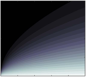
Figure 1(a) depicts the depth profile of the horizontal velocity component in the boundary layer, which constitutes the crucial convective term (2.32) in (2.31) for the leading-order temperature. Figure 1(b) shows the temperature field relative to the ambient water temperature, obtained by applying a finite difference scheme to the governing equation (2.31) and associated boundary conditions (2.33)–(2.34). Details of the numerical scheme are given in Appendix A.

Figure 1. (a) Profile of horizontal flow speed  $\tilde {u}(z)$. (b) Relative temperature field
  $T_R$ in the vertical plane
  $(x,z)$, for
  $A=0.3$ m,
  $T_b=20\,^{\circ }$C,
  $T_w=10\,^{\circ }$C,
  $\omega =1$ rad s
 $^{-1}$ and
  $h=5$ m. The thickness of the thermal boundary layer is
  $\delta _T\sim 2$ cm after
  $x\sim 10$ m.
Figure 1(b) shows that the thermal boundary-layer thickness – defined as the point at which the fluid temperature is 99 % of the ambient water temperature  $T_w$ – grows to approximately
  $2$ cm after
  $x\sim 10$ m. The growth of the boundary-layer thickness
  $\delta _T$ is initially very rapid, but slows as
  $x\gg 0$. This behaviour is also predicted by the analytical expression (2.42) which additionally provides several physical insights. For example, let us now consider the heat flux at the seabed. Figure 2(a) shows the behaviour of
  $q$ with horizontal distance
  $x$. The solid line represents the heat flux predicted by the numerical model based on the full governing equation (2.31), whereas the dashed line represents the analytical approximation (2.43). The latter successfully captures the behaviour of the heat flux, even though the analysis solely considers the first term in the Taylor expansion for the velocity
  $\tilde {u}$. The heat flux tends to infinity like
  $x^{-1/3}$ as
  $x$ approaches
  $0^+.$ This is due to the instantaneous increment of the temperature field with
  $z$ at
  $x=0^+$, as also shown in figure 1(b).

Figure 2. (a) Behaviour of heat flux  $q$ with horizontal distance along the seabed
  $x$. The continuous line represents the full numerical solution, whereas the dashed line represents the analytical result (2.43) based on a Taylor expansion of the forcing term
  $\tilde {u}$ as
  $z\rightarrow 0$. (b) Behaviour of normalised temperature
  $\varTheta (\eta )$ vs the non-dimensional variable
  $\eta =z\sqrt {|U|/(2x\nu) }$. Solid curve (‘Present model’) depicts the solution presented herein; dashed curve (‘White’) presents the corresponding case for the Blasius profile, see figures 4–9 of White (Reference White1991).
We now compare the numerical solution of (2.31) shown in figure 1(b) to a reference case of interest. Let us consider the flat-plate heat transfer process with velocity field described by the Blasius solution as in White (Reference White1991), with velocity at infinity equal to  $|U|$. Figure 2(b) shows the normalised temperature profile
  $\varTheta (\eta )$ (solid curve, ‘Present model’) evaluated according to the evolution equation for temperature (2.31) vs the normalised variable
  $\eta =z\sqrt {|U|/(2x\nu) }$. Note that we have used the numerical value of the Prandtl number for pure water,
 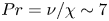 $Pr=\nu /\chi \sim 7$. Comparison with the Blasius solution (dashed curve, ‘White’) shows that the present model predicts larger values of the temperature field, even though the qualitative behaviour of the curves is similar. This highlights the importance of considering the complete velocity profiles (2.24)–(2.25) in the evolution equation (2.31).
Finally, we validate the analytical model by investigating the behaviour of the total heat flux  $Q$ over a fixed length
  $L=10$ m of seabed with varying wave frequency
  $\omega$ and different values of water depth
  $h$. Figure 3(a) shows
  $Q$ predicted by the finite difference numerical solver of the full convection–diffusion equation, whereas figure 3(b) shows the corresponding results from the analytical approximation (2.44). The two sets of results agree with each other qualitatively, indicating that the analytical model can be adopted for practical evaluations. Even so, it should be noted that the analytical model underpredicts heat flux, primarily because it underestimates the magnitude of the forcing term
  $\tilde {u}$.

Figure 3. Total heat flux  $Q$ as a function of wave frequency
  $\omega$ for different values of water depth
  $h$: (a) predictions by full numerical scheme and (b) analytical solution (2.44). The maximum of each curve is qualitatively predicted by the theoretical criterion (2.46), and all curves tend to zero as
  $\omega \rightarrow \infty$.
It is interesting to observe the presence of a maximum heat flux in each case. As the water depth  $h$ increases, this maximum heat flux occurs at progressively lower wave frequencies and longer wavelengths. This behaviour is captured explicitly by (2.46), which highlights the dependence on
  $h^{-1/2}$. Note also that all the curves tend to
  $Q=0$ at large values of wave frequency. In such cases, the term
  $\tilde {u}_0$ becomes very small and the governing equation (2.35a) can be approximated by
  $\partial ^2 T_1/\partial z^2\sim 0$. In other words, we require
  $\partial T_1/\partial z\sim 0$ to satisfy the condition at
  $z\rightarrow \infty$, so that heat transfer is absent. Therefore, short waves over moderate sea depths do not contribute to heat transfer at the seabed boundary layer.
4. Conclusions
We have investigated the mechanism of heat transfer in the boundary-layer region at the seabed. Using multiple-scale analysis and a perturbation approach, we first find the velocity field close to the seabed, then solve the governing convection–diffusion equation for fluid temperature. Given the small thermometric conductivity of water, large temperature gradients occur in the region close to the ocean bed. This simplifies the problem, enabling us to elucidate the effects of convection and diffusion at different orders, and to find the corresponding evolution equation for temperature.
We have also found an analytical expression for the temperature field based on an approximation of the streaming current in the bed boundary layer. The theoretical results shed light on the effect of surface waves on near-bed thermal transport processes. Specifically, they suggest that, rather than increasing monotonically with wavelength and phase speed, maximum heat transfer occurs at a finite value of wavelength which depends on the water depth. Given the spatial complexity of the velocity field, good agreement is achieved between the approximated analytical solution and predictions from a full numerical model based on a finite-difference scheme.
Our results provide a theoretical foundation for further applications to topics of considerable current interest, including biofouling (Vinagre et al. Reference Vinagre, Simas, Cruz, Pinori and Svenson2020), coral bleaching (Monismith Reference Monismith2007), cooling of underwater data centres (Cutler et al. Reference Cutler, Fowers, Kramer and Peterson2017), calibration of satellite data (Donlon et al. Reference Donlon, Minnett, Gentemann, Nightingale, Barton, Ward and Murray2002) and the emerging area of seawater air-conditioning solutions (Hunt, Byers & Sánchez Reference Hunt, Byers and Sánchez2019). For many of these applications, effects arising from turbulence, variable topography, more complex free-surface wave fields, Coriolis acceleration, internal waves, seabed mobility (e.g. ripples and dunes), etc. must be taken into account. These phenomena considerably complicate ocean heat-transfer mechanisms near the seabed, and would provide fruitful opportunities to extend the results discussed herein.
Acknowledgements
The authors are grateful to the referees for their constructive and helpful comments.
Funding
S.M. acknowledges support from EUROSWAC project funded by Interreg France (Channel) England Programme, project number 216. R.S. acknowledges support from EPSRC grant EP/V012770/1.
Declaration of interests
The authors report no conflict of interest.
Appendix A. Finite-difference scheme
In this section, we describe the finite-difference scheme to evaluate the steady solution of the boundary-value problem (2.31)–(2.33)–(2.34). We first define the temperature  $T_1(x_m,z_n)$ and forcing term
  $\tilde {u}(z_n)$ as
  $T_{m,n}$,
  $\tilde {u}_n$, whereas the
  $z$-derivative is evaluated using second-order central difference and
  $x$-integration conducted using a forward difference:
 \begin{equation} \frac{\partial T_1}{\partial x}=\frac{T_{m+1,n}-T_{m,n}}{\Delta x},\quad \frac{\partial^2 T_1}{\partial z^2}=\frac{T_{m,n+1}-2T_{m,n}+T_{m-1,n}}{\Delta z^2}. \end{equation}
Substitution into (2.31) yields
 \begin{equation} T_{m+1,n}=T_{m,n}+\frac{\chi \Delta x}{\tilde{u}_{n}\Delta z^2} \left(T_{m,n+1}-2T_{m,n}+T_{m,n-1}\right). \end{equation}
This algebraic expression is solved together with the boundary conditions in discrete form:
 \begin{equation} T_{0,n}=T_w,\quad T_{m,0}=T_b. \end{equation}
The forward scheme above is numerically stable for  $\chi \Delta x/(\tilde {u}_{n}\Delta z^2)\leq 1/2$ (Smith Reference Smith1985).
To investigate the convergence of the numerical solution, we evaluate the total heat flux  $Q$ for
  $A=0.3$ m,
  $T_b=20\,^{\circ }$C,
  $T_w=10\,^{\circ }$C,
  $\omega =1$ rad s
 $^{-1}$,
  $h=5$ m and different values of grid spacing
  $(\Delta z, \Delta x)$. These parameters correspond to the case represented in figure 1.
Figure 4 shows the behaviour of  $Q$ vs
  $\Delta z$, with corresponding values of
  $\Delta x$ assumed to be
  $\Delta x= \tilde {u}_{1}\Delta z^2/(2\chi)$ such that the stability criterion of the forward scheme is satisfied. The same figure shows that for
 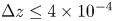 $\Delta z\leq 4\times 10^{-4}$ m and
  $\Delta x\leq 24\times 10^{-4}$ m, the numerical solution converges towards a fixed value. Grid spacing
  $(\Delta z, \Delta x)$ below which the solution converges depends on frequency
  $\omega$ and sea depth
  $h$. To reach convergence of the solution and avoid numerical instability for
  $\omega \in [0.25;2]$ rad s
 $^{-1}$, and
  $h\in [5; 10]$ m, in our evaluations we set
  $\Delta x=2\,{\times}\, 10^{-5}$ m and
  $\Delta z=3\times 10^{-4}$ m. These are the numerical values for the calculation shown in figure 3(a).

Figure 4. Behaviour of total heat flux  $Q$ vs spacing
  $\Delta z$ for
  $A=0.3$ m,
  $T_b=20\,^{\circ }$C,
  $T_w=10\,^{\circ }$C,
  $\omega =1$ rad s
 $^{-1}$ and
  $h=5$ m. Convergence of numerical solution is reached for
  $\Delta z\leq 4\times 10^{-4}$ m, whereas numerical stability requires
  $\Delta x\leq 24\times 10^{-4}$ m.


 Open access