


1. Introduction
The effect of a shock wave impinging on a supersonic boundary layer has been the subject of many studies, both experimental and theoretical. It is known that an instability forms in the separation region produced by the shock wave, and this typically causes the flow to undergo laminar–turbulent transition. The closely related experiments of Chapman, Kuehn & Larson (Reference Chapman, Kuehn and Larson1957) found that when a compressive feature such as a concave ramp is introduced into supersonic flow over an otherwise flat surface, a separation region occurs upstream. This phenomenon cannot be explained by the parabolic boundary layer equations, which permit only downstream propagation of disturbances. The theoretical explanation for this behaviour was eventually provided by (supersonic) triple-deck theory developed independently by Stewartson & Williams (Reference Stewartson and Williams1969) and Neiland (Reference Neiland1969). This theory provides a viscous–inviscid interaction problem that allows for upstream influence.
Following a formulation of the appropriate interactive equations, computational solutions to the problem of supersonic compression-ramp flow were sought eventually. The resulting flow is parametrised by a scaled measure ( $\alpha$) of the true ramp angle ( $\theta$), where
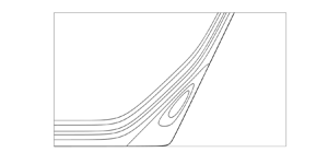
  $\alpha \propto \theta \,Re^{1/4}$; see e.g. Korolev, Gajjar & Ruban (Reference Korolev, Gajjar and Ruban2002). A schematic of the flow, which includes the scalings of the triple-deck model, is given in figure 1. The objective of the early studies of Rizzetta, Burggraf & Jensen (Reference Rizzetta, Burggraf and Jensen1979) and Ruban (Reference Ruban1978) was to determine steady-state solutions, though this was achieved by time-marching the unsteady triple-deck equations instead of solving directly the time-independent problem. The initial-value problem starts from a flat-plate solution, increasing the ramp angle to a final desired angle and time-marching until an approximate steady state is achieved. Owing to the limited computational resources of the time and the sensitive nature of the problem, only solutions for low to moderate values of $\alpha$ were obtained.

Figure 1. Schematic of the flow. The ramp is a distance  $L$ from the leading edge, and the triple-deck formulation spans a downstream scale of $O(L\,Re^{-3/8})$ around this point. The ramp angle $\theta$ for which interaction develops is $O(Re^{-1/4})$.
A different approach was taken by Smith & Khorrami (Reference Smith and Khorrami1991), who found steady-state solutions for much larger ramp angles up to  $\alpha =6.5$ by solving the steady equations directly. It was hypothesised therein that a critical ramp angle existed at which the steady flow developed a singularity; however, further studies of steady large-angle solutions by Korolev et al. (Reference Korolev, Gajjar and Ruban2002) and Logue (Reference Logue2008) suggest that this is not the case, though there is a slight quantitative discrepancy between their results at the largest ramp angles.
Instability of these flows has also been a topic of much theoretical investigation. It is known that supersonic flow is stable to Tollmien–Schlichting waves (see e.g. Duck Reference Duck1985); however, it has been shown by Tutty & Cowley (Reference Tutty and Cowley1986) that solutions to the triple-deck equations are in principle unstable to long-wavelength Rayleigh (LWR) waves for a variety of interaction conditions. These are inviscid instabilities where the wavelength is short compared to the triple-deck streamwise length scale, but remains long compared to the boundary-layer scale. If the flow is susceptible to such instabilities, then in any time-marching procedure, the growth of these waves will be limited only by the spatio-temporal resolution of the scheme – the better the resolution, the faster the waves will grow. Tutty & Cowley (Reference Tutty and Cowley1986) derived a general eigenrelation for the complex wavespeed  $c=c_r+{\rm i}c_i$, showing that (in the supersonic case) the presence of an inflection point (i.e. a point where $U_{YY}=0$) is a necessary but not sufficient condition for the flow to be unstable to LWR instabilities. For a supersonic base flow, the leading-order eigenrelation in the high-frequency limit is given by Tutty & Cowley (Reference Tutty and Cowley1986) as
 \begin{equation} \int_0^\infty\frac{U_{BY}}{((U_B+Y)-c)^2}\,\mathrm{d}Y +\frac{1}{c}=0, \end{equation}
where  $Y$ is the transverse coordinate, and $U_B+Y$ is the streamwise component of the base flow in the lower deck. These LWR modes have an asymptotically large frequency, therefore if the base flow is found as part of a time-marching procedure, then it can be treated quasi-steadily (and locally) at each time step due to the separation of scales. For a given base flow, this relation can be assessed at each streamwise location, and for an instability to be present, we require $c$ to have non-zero imaginary part in one or more regions. The above eigenrelation can be difficult to evaluate in the cases where the flow is stable or $c_i$ is numerically small, as the integral would have to be deformed into the complex $Y$-plane or be very close to a double pole, respectively.
Cassel, Ruban & Walker (Reference Cassel, Ruban and Walker1995) were the first to study these instabilities in compression-ramp flows. They obtained steady solutions to the unsteady equations by using a time-marching procedure in a manner similar to Rizzetta et al. (Reference Rizzetta, Burggraf and Jensen1979) and Ruban (Reference Ruban1978), this time for larger ramp angles. By abruptly increasing the ramp angle from a flat-plate solution to the desired value, a broad range of frequencies are excited so no artificial forcing is necessary to generate high-frequency instabilities. It was suggested that an absolute instability exists for  $\alpha \geqslant 3.9$, where it was stated that the first inflection points arise. Nevertheless, Cassel et al. (Reference Cassel, Ruban and Walker1995) were unable to connect the observed instability to the eigenrelation (1.1) derived by Tutty & Cowley (Reference Tutty and Cowley1986) for LWR modes, though it is clear from the comments therein that the authors did believe that the instabilities present were of this type.
The method of Cassel et al. (Reference Cassel, Ruban and Walker1995) was used later by Fletcher, Ruban & Walker (Reference Fletcher, Ruban and Walker2004) in an attempt to establish a connection between the numerically observed instability and the eigenrelation (1.1). Using substantially more refined spatial meshes and a spatially localised initial disturbance, it was argued that ramp angles in the region  $3.2 \leqslant \alpha \leqslant 3.7$ were convectively unstable, and larger angles were absolutely unstable. However, it had been stated previously by Cassel et al. (Reference Cassel, Ruban and Walker1995) that the flow was non-inflectional at these values of $\alpha$, which if true suggested that any convective instabilities must not be connected to the eigenrelation (1.1), a point that was later made by Logue, Gajjar & Ruban (Reference Logue, Gajjar and Ruban2014). In the case of absolute instability at larger values of $\alpha$, Fletcher et al. (Reference Fletcher, Ruban and Walker2004) found unstable solutions to (1.1) and compared the growth rate given by the eigenrelation (a value of 2.74) to the observed growth rate of the instability (a value of 0.74) in initial-value computations.
The contradictions in the literature can therefore be summarised as follows. Cassel et al. (Reference Cassel, Ruban and Walker1995) observed a high-frequency instability but could not connect it to (1.1). Fletcher et al. (Reference Fletcher, Ruban and Walker2004) observed convective instabilities for ramp angles  $3.2<\alpha <3.7$; however, (1.1) has a necessary condition of an inflection point in the flow, and Cassel et al. (Reference Cassel, Ruban and Walker1995) states that the flow becomes inflectional only above $\alpha \approx 3.9$. A comparison of the predicted/observed growth rates $c_i$ by Fletcher et al. (Reference Fletcher, Ruban and Walker2004) in the initial-value computation was not convincing (though inevitably such comparisons are difficult and depend on initial conditions). To try to resolve some of these issues, Logue et al. (Reference Logue, Gajjar and Ruban2014) investigated the problem by first solving the steady equations. Using this as a base flow, two linear problems were then investigated: first a global eigenvalue problem was derived, then convective instabilities were investigated via an initial-value problem. In the global eigenvalue problem, ramp angles up to $\alpha = 7.8$ were considered, but no unstable eigenvalues were found for any $\alpha$. The convective instabilities were investigated by introducing a localised disturbance at the wall and time-marching the linearised disturbance equations. This triggers a primary wavepacket which was well resolved in their computations; however, a secondary wavepacket remained unresolved for the range of spatio-temporal step sizes employed. For $\alpha > 3.2$, a continuous stream of wavepackets was formed in the separated region and grew rapidly in time, though a finer grid delayed the growth of these instabilities somewhat. It was stated that at the ramp angles for which the convective modes arose, the base flow remained non-inflectional so the instability could not be connected to the LWR instability of Tutty & Cowley (Reference Tutty and Cowley1986).
More recently, Exposito, Gai & Neely (Reference Exposito, Gai and Neely2021) employed the method of Cassel et al. (Reference Cassel, Ruban and Walker1995) to look at the influence of the precise choice of ramp shape. They found convective instabilities for even smaller slope angles than previously. Furthermore, they concluded that the instability was numerical as it was present only when the method of Cassel et al. (Reference Cassel, Ruban and Walker1995) was used to solve the ramp problem, whereas in Smith & Khorrami (Reference Smith and Khorrami1991) no such instability was encountered. However, it should be noted that as Smith & Khorrami (Reference Smith and Khorrami1991) solved only the steady equations, clearly no such temporal instability could ever be present in their solutions.
In this paper, we begin by solving the steady triple-deck equations via a global numerical method to obtain compression-ramp base flows, being careful to verify our results with the existing literature. We then consider linearised, unsteady perturbations to base flows at moderate ramp angles. It is instructive to first investigate the spatial instability problem by considering harmonic disturbances of a single frequency before returning to address temporal stability. By constructing a local eigenvalue problem, we investigate the growth rates of instabilities for large but finite wavenumbers/frequencies, before considering the asymptotic limit (in both the temporal and spatial problems, respectively).
2. Governing equations
We consider two-dimensional, high-Reynolds-number, supersonic flow over a ramp placed a distance  $L$ downstream from the leading edge of a flat plate, and define a Reynolds number $Re$ based on this length scale as shown in figure 1. The interacting flow at the base of the ramp is assumed to have streamwise extent $O(L\,Re^{-3/8})$, and upon using the triple-deck model, scaling the local shear out of the problem, and applying a Prandtl transform, we obtain the standard viscous–inviscid interaction problem of (Smith Reference Smith1973):
 $$\begin{gather} \frac{\partial U}{\partial T}+(U+Y)\,\frac{\partial U}{\partial X}+V\left(1+\frac{\partial U}{\partial Y}\right)={-}\frac{\partial P}{\partial X}+\frac{\partial^2U}{\partial Y^2}, \end{gather}$$
 $$\begin{gather}\frac{\partial P}{\partial Y}=0, \end{gather}$$
 $$\begin{gather}\frac{\partial U}{\partial X}+\frac{\partial V}{\partial Y}=0, \end{gather}$$
subject to the conditions
 $$\begin{gather} U=V=0\quad \mathrm{at}\ Y=0, \end{gather}$$
 $$\begin{gather}U\rightarrow A(X, T)+ F(X) \quad \mathrm{as}\ Y\rightarrow\infty, \end{gather}$$
 $$\begin{gather}U, V, P, A \rightarrow 0 \quad \mathrm{as} \ X\rightarrow -\infty, \end{gather}$$
 $$\begin{gather}P={-}\frac{\partial A}{\partial X}. \end{gather}$$
These are the unsteady triple-deck equations, with (2.2d) the interaction condition for supersonic flow; more explicit details can be found in e.g. Korolev et al. (Reference Korolev, Gajjar and Ruban2002). In this lower deck,  $(U+Y, V)$ is the velocity vector, $P$ is the pressure, $A$ is the displacement, and $F$ is the shape of the ramp. Strictly speaking, if we consider a sharp corner at the base of the ramp, then the function $F$ should take a piecewise definition:
 \begin{equation} F(X)=\begin{cases} 0 & X<0,\\ \alpha X & X>0, \end{cases} \end{equation}
where  $\alpha$ is the scaled acute angle between the ramp and the horizontal. However, to retain an everywhere differentiable wall shape (Rizzetta et al. Reference Rizzetta, Burggraf and Jensen1979), we follow the choice made by Cassel et al. (Reference Cassel, Ruban and Walker1995) and others, by using a slightly rounded corner:
 \begin{equation} F(X)=\frac{\alpha}{2}(X+\sqrt{X^2+r^2}), \end{equation}
where  $r$ is a constant. To enable comparisons to the existing literature, we take $r=0.5$, though the qualitative behaviour of the flow is consistent for other small values of $r$.
$r$.
2.1. Steady base flow solutions
A base flow is found from a direct solution of the steady form of (2.1)–(2.2), and denoted by  $(U,V,P,A) = (U_B,V_B,P_B,A_B)$, with $F$ defined as in (2.4). This system is solved using a novel numerical method. Given that there is upstream influence in (2.1) from the interaction condition (2.2d) (in addition to reversed flow in the corner of the compression ramp), we solve the steady problem by discretising over both $X$ and $Y$, and solving for all degrees of freedom simultaneously.
The numerical scheme used to solve the problem is relatively simple as we remain in primitive variable form. On a given spatial mesh  $(X_i, Y_j)$, $i=1, \ldots, N$, $j=1, \ldots, M$, in the range $i=2, \ldots, N-1$, $j=2, \ldots, M-1$ we evaluate (2.1a) at $(X_i, Y_j)$ using second-order central finite differences for both $X$ and $Y$ derivatives. When $i=N$, we again use central finite differences for the transverse derivative; however, we now use three-point backwards differencing for the streamwise derivatives. We evaluate (2.1c) at $(X_i, Y_{j-1/2})$ for $i=2, \ldots, N$, $j=2, \ldots, M$, again using second-order finite differences at all points, implementing backwards differencing in the streamwise direction when $i=N$. When $i=1$, we impose (2.2c) as Dirichlet conditions. For the interaction condition (2.2d), we use central finite differences, except at the final streamwise location, where we require
 \begin{equation} \frac{\partial P_B}{\partial X}=0 \quad \mathrm{at} \ X=X_N, \end{equation}
where  $X_N$ is the furthest downstream streamwise location.
We solve the resulting discrete system numerically using Newton iteration, where each iteration requires the inversion of a sparse  $2N(M+1) \times 2N(M+1)$ linear system. For all the results given herein, we use a uniform mesh in the transverse direction with $Y_{max}=50$ and a remapped mesh in the streamwise direction in order to concentrate points in the corner region. The typical grid size is ( $3001\times 601$); however, results were reproduced to graphical accuracy for grids ( $1601\times 601$) and ( $1601\times 301$).
2.1.1. Base flow results
To demonstrate that this global numerical method solves the problem accurately, we will give a brief comparison of our results to the existing literature of the steady problem, before considering the important flow features. Our first comparison is with Logue et al. (Reference Logue, Gajjar and Ruban2014) for  $\alpha =3.6$. Figure 2(a) shows the surface shear stress associated with the base flow
 \begin{equation} \tau_0(X)=U_{BY}(X, Y=0)+1, \end{equation}
together with data extracted from figure 7 of Logue et al. (Reference Logue, Gajjar and Ruban2014). The flow becomes separated at  $X \approx -7.5$ and does not reattach until $X \approx 7$, though in between these values there is a local maximum at $X\approx 0$. The minimum of $\tau _0$ upstream of this maximum is only a local minimum, with the global minimum lying further downstream where the strongest reversed flow is expected to be. As $\alpha$ is increased, we expect that the local maximum will grow in value until eventually we will have $\tau _0>0$ at this point, leading to secondary separation.

Figure 2. Steady solutions for the wall shear  $\tau _0$: (a) $\alpha =3.6$, (b) $\alpha =4.5$. The solid line indicates the present method; dots indicate Logue et al. (Reference Logue, Gajjar and Ruban2014), and crosses indicate Korolev et al. (Reference Korolev, Gajjar and Ruban2002).
The other comparison made is with Korolev et al. (Reference Korolev, Gajjar and Ruban2002) for  $\alpha =4.5$. This is the lowest ramp angle given therein, and the two methods outlined in that paper gave very similar results to graphical accuracy. Figure 2(b) again shows $\tau _0$ for this value of $\alpha$. We see that our results show good agreement with theirs for this relatively large value of $\alpha$, even for the complicated behaviour within the separation region. Here, the local maximum has grown such that $\tau _0$ is just smaller than zero, so the flow is on the cusp of developing a region of secondary separation.
For a typical computational solution over a truncated domain, even at  $\alpha =3.6$ the base flow can be ‘weakly inflectional’ in the sense that inflection points are displaced substantially from the ramp surface where $\vert U_{BY} \vert$ is numerically very small ( $10^{-5}$ and smaller). In agreement with Cassel et al. (Reference Cassel, Ruban and Walker1995), only at larger ramp angles $\alpha >3.8$ do we obtain robust inflectional points close to the boundary in the recirculation region. Using these base flows, we can seek solutions to (1.1) for each value of $\alpha$. However, for $\alpha =3.6$, no unstable solutions for $c$ can be found at any streamwise location. As a check, we also solve the discretised LWR equation directly as an eigenvalue problem using finite difference methods; again, no complex $c$ solutions were found.
The results of Logue et al. (Reference Logue, Gajjar and Ruban2014) demonstrate an instability in their initial-value computations for  $\alpha =3.6$; however, it is evidently not described by the eigenrelation (1.1). The rest of this paper will be focused on determining the nature of this instability.
2.2. Linear perturbations
We introduce linear perturbations to the steady base flow of the form
 $$\begin{gather} U=U_B(X,Y)+\varepsilon\,U_p(X, Y, T)+\cdots, \end{gather}$$
 $$\begin{gather}V=V_B(X, Y)+\varepsilon\,V_p(X, Y, T)+\cdots, \end{gather}$$
 $$\begin{gather}P=P_B(X)+\varepsilon\,P_p(X, T)+\cdots, \end{gather}$$
 $$\begin{gather}A=A_B(X)+\varepsilon\,A_p(X, T)+\cdots, \end{gather}$$
where  $\varepsilon \ll 1$. Upon substitution into (2.1)–(2.2), we find that the perturbation terms satisfy
 $$\begin{gather} \frac{\partial U_p}{\partial T}+(U_B+Y)\,\frac{\partial U_p}{\partial X}+U_p\,\frac{\partial U_B}{\partial X}+V_p\left(1+\frac{\partial U_B}{\partial Y}\right)+V_B\,\frac{\partial U_p}{\partial Y}={-}\frac{\partial P_p}{\partial X}+\frac{\partial^2 U_p}{\partial Y^2}, \end{gather}$$
 $$\begin{gather}\frac{\partial U_p}{\partial X}+\frac{\partial V_p}{\partial Y}=0, \end{gather}$$
subject to the conditions
 $$\begin{gather} U_p=V_p=0\quad \mathrm{at}\ Y=0, \end{gather}$$
 $$\begin{gather}U_p, V_p, P_p, A_p \rightarrow 0\quad \mathrm{as}\ X\rightarrow-\infty, \end{gather}$$
 $$\begin{gather}U_p\rightarrow A_p, \quad \frac{\partial U_p}{\partial Y}\rightarrow0, \quad \mathrm{as} \ Y\rightarrow\infty, \end{gather}$$
 $$\begin{gather}P_p={-}\frac{\partial A_p}{\partial X}. \end{gather}$$
Solutions to (2.8)–(2.9) are obtained by a second-order discretisation in time, in addition to the methodology described in § 2.1. We will consider the receptivity problem by relaxing the impermeability condition at the surface.
As a brief demonstration of the issues encountered when time-marching this linear problem, we consider a case similar to that of Logue et al. (Reference Logue, Gajjar and Ruban2014), and transiently force a response for a short time. In this case, we replace the impermeability condition by
 \begin{equation} V_p(X, 0, T)=T^2\exp({-50T})\,(X-X_0) \exp({-\gamma (X-X_0)^2}), \end{equation}
where  $X_0$ and $\gamma$ are constants to be chosen. For this test case, we take $X_0=-5$, $\gamma =3$. Other choices can be made for a perturbation here; for example, Logue et al. (Reference Logue, Gajjar and Ruban2014) choose to impose a perturbation to the no-slip condition at the wall. In our case, perturbing the system via the impermeability condition reproduces the same qualitative features described by Logue et al.
Figure 3 shows the scaled surface shear stress for the perturbation  $\tau _p=\partial U_p/\partial Y$ (evaluated at $Y=0$) for increasing times and a base flow with $\alpha =3.6$. We see in figure 3(a) that an initial wavepacket develops from the injection site, and in figure 3(b) this is seen to have grown by several orders of magnitude after it has been convected downstream. This growth slows as the wavepacket moves into a less unstable part of the flow. In figure 3(c), the maximum amplitude of this wave has grown by only one order of magnitude, and by this time it is clear that there are some new oscillations upstream of the primary wavepacket. These new oscillations are higher in frequency and are growing at a faster rate; at $T=1.75$, they are larger in amplitude than the primary wavepacket. This secondary wavepacket was found by Logue et al. (Reference Logue, Gajjar and Ruban2014) to be grid-dependent, and they were unable to resolve it, leading to mesh-dependent results.

Figure 3. Evolution of the surface stress perturbation for base flow of  $\alpha =3.6$ at various times: (a) $T=0.5$, (b) $T=1$, (c) $T=1.6$ and (d) $T=1.75$.
3. Spatial instability
As seen in § 2.2, any initial-value calculation will naturally excite waves of all frequencies. If the flow is unstable to large frequencies, then at best we will only be able to time-march the solution for so long before this high-frequency growth will dominate the calculation. To gain an insight into the growth of the instability, we instead begin by considering the effect of single-frequency forcing. We will focus on the case  $\alpha =3.6$, and examine a spatial problem to describe how the forced response develops downstream through the compression-ramp flow.
3.1. A harmonic problem
We consider a linear, harmonic perturbation to the base flow in the case  $\alpha =3.6$ so that the impermeability condition is replaced by
 \begin{equation} V_p(X, 0, T)=\exp({-{\rm i}\omega T})\,(X-X_0) \exp({-\gamma (X-X_0)^2}), \end{equation}
where  $\omega$ is the frequency of the forcing, and $X_0$ and $\gamma$ are constants to be chosen. Forcing of this nature suggests that we search for solutions to the system (2.8)–(2.9) of the form
 \begin{equation} (U_p,V_p,P_p,A_p)=\exp({-{\rm i}\omega T})\left ( U_H(X, Y),V_H(X, Y),P_H(X),A_H(X)\right ). \end{equation}
The system to be solved is then
 $$\begin{gather} -{\rm i}\omega U_H+(U_B+Y)\,\frac{\partial U_H}{\partial X}+U_H\,\frac{\partial U_B}{\partial X}+V_H\left(1+\frac{\partial U_B}{\partial Y}\right) +V_B\,\frac{\partial U_H}{\partial Y}={-}\frac{\mathrm{d}P_H}{\mathrm{d} X}+\frac{\partial^2 U_H}{\partial Y^2}, \end{gather}$$
 $$\begin{gather}\frac{\partial U_H}{\partial X}+\frac{\partial V_H}{\partial Y}=0, \end{gather}$$
 $$\begin{gather}P_H(X)={-}A_H'(X), \end{gather}$$
 $$\begin{gather}U_H=0, \quad V_H=(X-X_0) \exp({-\gamma (X-X_0)^2})\quad \mathrm{at}\ Y=0, \end{gather}$$
 $$\begin{gather}U_H, V_H, P_H, A_H\rightarrow0 \quad \mathrm{as}\ X\rightarrow-\infty, \end{gather}$$
 $$\begin{gather}U_H\rightarrow A_H,\quad \frac{\partial U_H}{\partial Y}\rightarrow 0 \quad \mathrm{as}\ Y\rightarrow\infty. \end{gather}$$
Like the base flow calculation (see § 2.1) this problem is then formulated globally, and being linear, it can be solved for all degrees of freedom simultaneously in a single matrix inversion.
We begin by considering the effect of varying  $\omega$ on the behaviour of the solutions. Figure 4 shows the real part of the (harmonic) scaled surface shear stress perturbation $\tau _H = \partial U_H/\partial Y$ (on $Y=0$) for various $\omega$ with $X_0 = -5$, $\gamma = 3$ in (3.1). As $\omega$ is increased, a wavepacket with increasing amplitude is formed (with the expected decrease in wavelength). This behaviour was found to be grid-independent for sufficiently fine meshes, though large numbers of streamwise points (typically 3001 nodes) were required to confirm this for $\omega >16$.

Figure 4. The distribution of the real part of the scaled surface shear stress of the harmonic perturbation  $\tau _H$ forced by (3.1) for increasing frequency $\omega$ with $X_0=-5$, $\gamma =3$ and ramp angle $\alpha =3.6$: (a) $\omega =8$, (b) $\omega =16$, (c) $\omega =24$ and (d) $\omega =32$.
If we assume naively that the spatially developing waves shown in figure 4 have sufficient scale separation from the base flow, then we can define a local complex wavenumber to be
 \begin{equation} K={-}\frac{{\rm i}}{\tau_H}\,\frac{\mathrm{d}\tau_H}{\mathrm{d}X}. \end{equation}
Figures 5(a) and 5(b) show  $-K_i$ and $K_r$ (where $K=K_r+{\rm i}K_i$), respectively, for increasing forcing frequency $\omega$. Here, $-K_i$ is the local spatial growth rate of the disturbance. Quantitatively similar results are found when varying the disturbance generator through $X_0$ and $\gamma$. We see that in the separation region, the instability undergoes spatial growth before eventually decaying further downstream, in line with figure 4.

Figure 5. (a) The local spatial growth rate, and (b) the wavenumber, of the harmonic disturbance. The blue dotted line indicates  $\omega =8$, the orange dot-dashed line indicates $\omega =16$, the purple dashed line indicates $\omega =24$, and the black solid indicates $\omega =32$.
These results are well-resolved and point to an underlying eigenvalue problem governing the spatial behaviour of the disturbance. The base flow appears to be unstable at these values of  $\omega$; nevertheless, as discussed in § 2.2, in the high-frequency limit the eigenrelation (1.1) does not give unstable modes (in either the spatial or temporal cases).
3.2. A local spatial eigenvalue problem
To formally connect the linear harmonic problem considered above to the asymptotically large-frequency limit, we study a local eigenvalue problem. Instead of the receptivity problem driven by injection, we instead look directly for propagating normal mode solutions
 \begin{equation} (U_p,V_p,P_p,A_p) = \exp({{\rm i}(KX-\omega T)}) ( \tilde{U}(Y),\tilde{V}(Y),\tilde{P},\tilde{A} ); \end{equation}
in this approach, the shape functions remain parametrically dependent on  $X$ through the local base flow, but we do not show this dependence explicitly. This assumption is rational only in the high-frequency limit where there is sufficient scale separation between the base flow and the perturbations, so the resulting eigenvalue problem can be evaluated locally. Upon substitution into the governing equations, we obtain the local eigenvalue problem
 $$\begin{gather} -{\rm i}\omega \tilde{U}+{\rm i}K (U_B+Y) \tilde{U}+\tilde{U}\,\frac{\partial U_B}{\partial X}+V_B\, \frac{\mathrm{d}\tilde{U}}{\mathrm{d}Y}+\tilde{V}\left(1+\frac{\partial U_B}{\partial Y}\right)={-}{\rm i} K \tilde{P}+\frac{\mathrm{d}^2\tilde{U}}{\mathrm{d}Y^2}, \end{gather}$$
 $$\begin{gather}{\rm i}K \tilde{U}+\frac{\mathrm{d}\tilde{V}}{\mathrm{d}Y}=0, \end{gather}$$
 $$\begin{gather}\tilde{U}=\tilde{V}=0 \quad \mathrm{at}\ Y=0, \end{gather}$$
 $$\begin{gather}\tilde{U}\rightarrow \tilde{A} \quad \mathrm{as}\ Y\rightarrow\infty, \end{gather}$$
 $$\begin{gather}\tilde{P}={-}{\rm i}K \tilde{A}. \end{gather}$$
We choose to neglect the non-parallel terms in (3.6a), but the viscous term is retained to regularise any critical layers. This problem is localised to each streamwise location, and we are free to normalise the eigenfunctions. On taking  $\tilde {A}\equiv 1$, (3.6a) and (3.6d) become
 $$\begin{gather} - {\rm i}\omega \tilde{U}+{\rm i}K (U_B+Y) \tilde{U}+\tilde{V}\left(1+\frac{\partial U_B}{\partial Y}\right)={-}K^2 +\frac{\mathrm{d}^2\tilde{U}}{\mathrm{d}Y^2}, \end{gather}$$
 $$\begin{gather}\tilde{U}\rightarrow1\quad \mathrm{as}\ Y\rightarrow\infty, \end{gather}$$
after eliminating  $\tilde {P}$ using the interaction condition (3.6e). To solve this problem numerically requires a truncation of the domain to $Y\in [0,Y_\infty ]$, and for solutions to be independent of the truncation $Y_\infty$, we also require that the correct far-field behaviour is achieved asymptotically with
 \begin{equation} \frac{\mathrm{d}\tilde{U}}{\mathrm{d}Y}\rightarrow 0 \quad \mathrm{as}\ Y\rightarrow \infty. \end{equation}
Given a frequency of the disturbance,  $\omega$, we can now solve (3.7a), (3.6b) subject to (3.6c), (3.7b) and (3.8) to determine the eigenvalue $K$.
$K$.
Starting with  $\omega =32$, an initial guess for $K$ can be found at any $X$ location by applying (3.4) to the harmonic results. Figures 6(a) and 6(b) compare the $K$ values obtained from this local eigenvalue problem with those obtained from the harmonic spatially developing disturbance. The two results show good agreement, even at this rather modest value of frequency. As a check, we then look at examples of the eigenfunctions $\tilde {U}$ alongside appropriately scaled eigenfunctions $U_H$ from the linear harmonic problem. In figures 6(c) and 6(d), we see that the eigenfunctions display the same type of behaviour in both problems, and in particular at $X\approx 0$ the agreement is very good. Close to the wall, there is a thin Stokes layer developing at high frequencies; we will return to this feature below.

Figure 6. Comparison of (a)  ${\rm Im}(K)$ and (b) ${\rm Re}(K)$ produced by the linear harmonic approach (dashed line) and the local eigenvalue problem (solid line), and the real part of the scaled eigenfunctions $\tilde {U}$ (solid line), $U_H$ (dashed line) at (c) $X=0.0045$, (d) $X=6$, for $\omega =32$.
There are unstable eigenvalues for a finite streamwise  $X$ range around the corner of the ramp. Figure 7 shows the variation of the dominant ${\rm Im}(K)$ as a function of $X$ location for a range of increasing frequency $\omega$. Whilst the extent of the region of instability is reduced slightly, there remains a large region for which there are unstable solutions to the local eigenvalue problem. In addition, the maximal growth rate is at $X\approx 0$ at the larger values of $\omega$ considered, with $K_i\approx -12$. This growth rate shows no evidence of growing linearly as $\omega$ increases, hence it cannot be captured by the eigenvalue problem (1.1), which describes modes for which the growth rate is $O(\omega )$ when $\omega \gg 1$.

Figure 7. Imaginary part of  $K$ against streamwise location $X$ for varying disturbance frequency $\omega$ in the case $\alpha =3.6$. These results are obtained from the local eigenvalue problem (3.6); negative values indicate downstream spatial growth.
We now consider how the growth rate changes at a fixed streamwise location as  $\omega$ increases. In figure 8, there are two different types of behaviour: ${\rm Im}(K)$ initially decreases before reaching a clear maximum growth rate, then increases until it eventually becomes greater than zero (and hence stable) for sufficiently large $\omega$; or ${\rm Im}(K)$ decreases until it plateaus, then does not appear to have a well-defined maximum growth rate. The second type of behaviour could be problematic, as the peak growth rate is found only for high frequency.

Figure 8. Imaginary part of  $K$ against disturbance frequency $\omega$ for various streamwise locations $X$ in the case $\alpha =3.6$. The blue dotted line indicates $X=-4.83$, the black solid line indicates $X=-0.05$, the red dashed line indicates $X=1.16$, and the purple dot-dashed line indicates $X=3.05$. These results are obtained from the local eigenvalue problem (3.6); negative values indicate downstream spatial growth.
It is difficult to ascertain the asymptotic behaviour of  ${\rm Im}(K)$ in the limit $\omega \rightarrow \infty$ from the local eigenvalue problem because of the Stokes layer. This layer has decreasing thickness $O(\omega ^{-1/2})$ (see § 3.3), therefore it becomes increasingly difficult to resolve.
3.3. The large-frequency limit
We now consider the same local eigenvalue problem for frequencies that are asymptotically large. Evaluating the streamwise momentum equation (3.6a) near the wall, we require a Stokes layer with thickness  $Y=\omega ^{-1/2} \eta$, where $\eta =O(1)$. In the Stokes layer, the solutions take the form
 \begin{equation} \tilde{U}=\omega U_S+\cdots, \quad \tilde{V}=\omega^{3/2}V_S+\cdots. \end{equation}
For a wave that propagates at the speed of the underlying base flow, we require that
 \begin{equation} K=\omega K_0+\cdots, \end{equation}
where  $K_0$ is related to the inverse of the phase speed. The Stokes layer problem results in
 $$\begin{gather} U_S={-}{\rm i}K_0^2(1-{\rm e}^{-\sqrt{-{\rm i}}\,\eta} ), \end{gather}$$
 $$\begin{gather}V_S={-}K_0^3\left(\eta+\frac{1}{\sqrt{-{\rm i}}}({\rm e}^{-\sqrt{-{\rm i}}\,\eta}-1)\right). \end{gather}$$
As we leave the Stokes layer (i.e in the limit  $\eta \rightarrow \infty$), we have
 $$\begin{gather} U_S\rightarrow -{\rm i}K_0^2, \end{gather}$$
 $$\begin{gather}V_S\rightarrow -K_0^3 \eta +\frac{K_0^3}{\sqrt{-i}}. \end{gather}$$
We now return to finding solutions in the lower deck of the triple-deck structure. The Stokes layer solution suggests that in the lower deck we should expand  $\tilde {U}$, $\tilde {V}$ as
 \begin{equation} \tilde{U}=\omega U_l+\cdots, \quad \tilde{V}=\omega^2 V_l+\cdots. \end{equation}
The second term in (3.12b) suggests that there will be an  $O(\omega ^{3/2})$ correction term to $\tilde {V}$, and therefore an $O(\omega ^{1/2})$ correction to $\tilde {U}$ and $K$. Substituting in the leading-order expansions to the perturbation equations gives the problem
 $$\begin{gather} -{\rm i} U_l+{\rm i}K_0 (U_B+Y) U_l+V_l\left(1+ \frac{\partial U_B}{\partial Y}\right)={-}K_0^2, \end{gather}$$
 $$\begin{gather}{\rm i} K_0 U_l+\frac{\mathrm{d}V_l}{\mathrm{d}Y}=0, \end{gather}$$
subject to the matching conditions with the Stokes layer and
 \begin{equation} U_l\rightarrow 0, \quad \frac{\mathrm{d}U_l}{\mathrm{d}Y}\rightarrow 0 \quad \mathrm{as}\ Y\rightarrow\infty. \end{equation}
This problem differs from the large but finite frequency version of the local eigenvalue problem by the fact that  $U_l$ decays in the far field.
To find non-trivial solutions to this problem, we can either solve the above generalised eigenvalue problem directly, or equivalently look for solutions to the eigenrelation
 \begin{equation} 0=\int_0^\infty \frac{U_{BY}}{(1-K_0 (U_B+Y))^2}\,\mathrm{d}Y+\frac{1}{K_0}, \end{equation}
which comes from eliminating  $U_l$ in favour of $V_l$ and integrating (3.14). This eigenrelation is simply the spatial analogue of the relation (1.1), with complex $K_0$ solutions corresponding to spatial instabilities of the base flow. However, this eigenrelation has no unstable complex roots, which is consistent with the bounded growth rates obtained in the large-frequency limit, as shown in figure 8.
This suggests that in the high-frequency limit, the wavenumber expands as
 \begin{equation} K=\omega K_{0}+O(\omega^{1/2}), \end{equation}
where no solution has been found with  ${\rm Im}(K_0)<0$. We will return to the limiting problem in § 5 in the context of a temporal stability problem.
4. Temporal instability
Whilst the spatial problem is simpler to validate against the full triple-deck formulation, the temporal problem is of more relevance to the initial-value computations discussed in the wider literature.
4.1. A local eigenvalue problem
Returning to the local eigenvalue problem (3.6), we fix the real wavenumber  $K$ and iterate to find a complex frequency $\omega$. If $\omega$ has a positive imaginary part, then the base flow will be unstable at this streamwise location to waves with the corresponding wavenumber $K$ and phase speed $c_r={\rm Re}(\omega )/K$. This approach is rational only in the large wavenumber limit; however, at moderate values values of $K$, the results can be checked against an initial-value calculation, and we return to this in § 4.2.
Figure 9 shows the downstream behaviour of  ${\rm Im}(\omega )$. It is clear that as $K$ increases, the region of instability is reduced slightly. However, for the larger values of $K$, the growth rate peaks near to $X=0$, a behaviour similar to the spatial analogue.

Figure 9. Imaginary part of the complex frequency  $\omega$ against streamwise location $X$ for various disturbance wavenumbers $K$ for a base flow with $\alpha =3.6$. These results are obtained from the local eigenvalue problem (3.6), and positive values indicate temporal growth of the disturbance.
Figure 10(a) shows the growth rate  ${\rm Im}(\omega )$ variation with $K$ at fixed streamwise locations. As in the spatial problem, sufficiently far from the corner, a local temporally stable flow is obtained for large $K$, but near to $X=0$, an instability exists. It is not surprising that the presence of these unstable modes causes substantial difficulties for finite-resolution computations, but the fact that this growth rate appears to remain bounded for larger values of $K$ again means that it cannot be obtained from the eigenrelation (1.1). Figure 10(b) shows that the phase speed $c_r={\rm Re}(\omega )/K$ tends to a constant value as $K$ increases.

Figure 10. Behaviour of the temporal growth rate and phase speed against the disturbance wavenumber  $K$ for various streamwise locations $X$: (a) growth rate ${\rm Im}(\omega )$, (b) phase speed $c_r={\rm Re}(\omega )/K$. The blue dotted line indicates $X=-4.83$, the black solid line indicates $X=-0.05$, the red dashed line indicates $X=1.16$, and the purple dot-dashed line indicates $X=3.05$. These are obtained from the local eigenvalue problem (3.6). In (a), positive values indicate temporal growth of the disturbance.
As expected, the temporal local eigenvalue problem is comparable to the spatial analogue. For large, finite  $K$ there is a finite region around the corner where the flow is unstable, and the maximal growth rate remains large for the wavenumbers considered in this section.
4.2. Initial-value problem
Any computation of the linear initial-value problem will eventually be dominated by the high-wavenumber components present in the initial conditions, as these are the fastest growing. To mitigate this, we will force a response in the linear perturbation equations (2.8)–(2.9) by replacing the impermeability condition with an expression that is dominated by a single wavenumber component. As the flow appears to be most unstable in the region of reversed flow, we ensure that the perturbation has fixed wavelength in this region, so the impermeability condition is now replaced by a transient forcing:
 \begin{equation} V(X, 0, T)=\begin{cases} T^2\,{\rm e}^{{-}50 T} \sin (KX) & |X|<20,\\ 0 & |X|>20, \end{cases} \end{equation}
where  $K$ is an integer multiple of ${\rm \pi}$. The discontinuity in the derivative of this condition will introduce high-frequency/short-wavelength noise into the problem that will eventually dominate the solution; however, over moderate times, the effect of this should be negligible in the corner ( $X\approx 0$) region. We can now determine an approximate phase speed and temporal growth of these waves, for comparison with the local eigenvalue problem studied above. For the sake of comparison, we take $K=2{\rm \pi}$ in both the initial-value problem and the local eigenvalue problem.
We will use the scaled perturbation surface shear stress  $\tau _p(X,T)=\partial U_p/\partial Y$ (on $Y=0$) as a measure of the perturbation, and distributions are shown at $T={\rm \pi} /20$ and $T=3{\rm \pi} /10$ in figure 11. At early times ( $T={\rm \pi} /20$), there is clearly growth of the initial perturbation as it develops through the corner region; at later times ( $T=3{\rm \pi} /10$), the disturbance has been convected downstream whilst undergoing growth of four orders of magnitude. Because we have limited the initial disturbance wavenumber, this response remains well-resolved over this time scale. Our goal is to see whether the local eigenvalue problem accurately predicts the growth rate and phase speed of these waves.


Figure 12 shows a contour plot of  $\tau _p(X,T)$ in the corner region for ${\rm \pi} /20\leqslant T\leqslant 3{\rm \pi} /20$. Superimposed are two lines with a gradient that corresponds to the maximum phase speed (calculated from the local eigenvalue problem (3.6)) either side of a downstream-propagating maximum of $\tau _p$. We see that the disturbance developing in the initial-value computations is travelling at approximately the phase speed determined from the local eigenvalue problem.

Figure 12. Contours of the perturbation shear  $\tau _p$ for ${\rm \pi} /20\leqslant T\leqslant 3{\rm \pi} /20$. The black lines show the phase speed of propagation predicted from the local eigenvalue problem at $X=0$.
To compare the temporal growth of the instability, we examined how a local maximum of  $\tau _p$ shown in figure 11(a) increases in amplitude. To do this, we follow a maximum $\tau _M$ starting at $T={\rm \pi} /20$, and estimate the amplitude at the next time to be
 \begin{equation} \tau_M(T + \Delta T)=\tau_M(T) \exp({\sigma(X_M)\,\Delta T}), \end{equation}
where  $\sigma (X_M)$ is the temporal growth rate according to the local eigenvalue problem at the corresponding $X=X_M$ location of this maximum in the initial-value computation results. We then repeat this procedure until we reach the desired final time. Figure 13 compares the predicted and calculated growth of $\tau _M$ up to the time $T=3{\rm \pi} /10$. The prediction (4.2) is approximate at this (not particularly large) value of $K=2{\rm \pi}$ as there remain both non-parallel contributions and a slow evolution of local wavenumber; nevertheless, there remains good agreement with results from the initial-value computation.

Figure 13. A comparison of the predicted wave growth in the linear initial-value problem (blue) with that predicted by the local temporal eigenvalue problem (black).
4.3. The large wavenumber limit
The large wavenumber limit  $K\rightarrow \infty$ follows that of § 3.3. Again, close to the wall there is a Stokes layer of thickness $Y=K^{-1/2} \xi$, where $\xi =O(1)$. Here we obtain the eigenrelation (1.1):
 \begin{equation} 0=\int_0^\infty \frac{U_{BY}}{(\omega_0-(U_B+Y))^2}\,\mathrm{d}Y+\frac{1}{\omega_0}. \end{equation}
When  $\alpha =3.6$ and $X=0$, we can find no unstable solutions to this eigenproblem, yet a growing instability is observed in the initial-value computations of figure 11. For larger values of $\vert X\vert$ (further from the corner), we can find stable solutions ( ${\rm Im}(\omega _0)<0$) via analytic continuation of the base flow $U_B$ to a deformed contour of $Y$ in the lower half-plane, consistent with the stable results for $X=-4.83, 3.05$ shown in figure 10(a). However, these leading-order decay rates approach zero rapidly on approaching the corner region.
Hence for  $\alpha =3.6$ in the large-wavenumber limit, the complex frequency appears to expand like
 \begin{equation} \omega=K \omega_{0} +O(K^{1/2}), \end{equation}
with  ${\rm Im}(\omega _0)\leqslant 0$, being numerically indistinguishable from zero when sufficiently close to the corner region. In this case a higher-order correction term that is not determined by the integral relation (1.1) dominates the temporal growth. Therefore, any attempt to correlate (unstable) temporal growth rates obtained in initial-value computations with (1.1), such as those in Fletcher et al. (Reference Fletcher, Ruban and Walker2004), is possible only at larger ramp angles, e.g. $\alpha =4.5$, where ${\rm Im}(\omega _0)>0$.
5. Discussion
The triple-deck formulation for supersonic flow over a compression ramp has been discussed a number of times over the last 30 years. Unsteady results for this problem are consistently dominated by growing high-frequency perturbations as the ramp angle parameter ( $\alpha$) is increased. Nevertheless, the origin of these waves has remained largely unexplained, being attributed either to the eigenrelation (1.1) (Cassel et al. Reference Cassel, Ruban and Walker1995; Fletcher et al. Reference Fletcher, Ruban and Walker2004) or more recently to a numerical instability of the discretised problem by Exposito et al. (Reference Exposito, Gai and Neely2021). A necessary condition for the instability described by (1.1) is that the flow is inflectional, and Cassel et al. (Reference Cassel, Ruban and Walker1995) indicated that base flows were non-inflectional for $\alpha < 3.9$. This added a further inconsistency since the results of Fletcher et al. (Reference Fletcher, Ruban and Walker2004) and Logue et al. (Reference Logue, Gajjar and Ruban2014) clearly show instability in the corner region of the ramp, even in this moderate angle regime. Furthermore, as shown by Logue et al. (Reference Logue, Gajjar and Ruban2014), although initial development of a wavepacket arising from a localised transient disturbance was robust and reproducible, a secondary higher-frequency wavepacket was observed, which remained unresolved even on the finest spatial/temporal meshes reported.
In this work, we have tackled the supersonic compression ramp using a global numerical method to find both steady equilibrium states and then determine their linear spatial/temporal stability. As in previous studies, attempts to connect the spatial or temporal growth of the instability to the leading-order eigenrelation (1.1) were unsuccessful for the moderate ramp angles ( $\alpha \leq 3.6$) considered herein.
Unstable solutions to (1.1) must grow at a rate that increases without bound as the inverse of the wavelength, whereas in the compression ramp at moderate ramp angles this is not the case, as shown in figure 10 for  $\alpha =3.6$. As the ramp angle is reduced further, this maximum growing mode eventually moves to a finite wavenumber before the instability is removed entirely. For example, at a lower angle $\alpha =3$, the peak growth can be found for a wavenumber $K\approx 130$; nevertheless, to resolve this scale would still require a computational mesh sufficiently fine to resolve a perturbation wavelength $2{\rm \pi} /130\approx 0.048$.
The local temporal eigenvalue problem (3.6) is based on a large-wavenumber assumption that neglects non-parallelism but still retains the viscous term. We have confirmed that the solutions of this (ad hoc) viscous temporal eigenvalue problem do recover the formal inviscid solution for  $K\gg 1$. To do this, we use the phase speed $\omega _{0r}$ determined in the large- $K$ limit (i.e. from figure 10b) as an initial guess in solving the inviscid leading-order eigenproblem calculated over a complex $Y$ contour deformed appropriately at the critical layer. Figure 14 displays the value of $\omega _{0r}$ for increasing values of $K$ over a range of streamwise locations alongside the inviscid solution. As expected, the two solutions show very good agreement for $K$ sufficiently large, and at $K=500$ they are the same to graphical accuracy.

Figure 14. Comparison of  $\omega _{0r}$ from the local (viscous) temporal eigenproblem (3.6) for various disturbance wavenumbers $K$, compared with the formal leading-order inviscid solution. The blue dot-dashed line indicates $K=100$, the purple dashed line indicates $K=200$, the red solid line indicates $K=500$, and data points are the inviscid results.
At a fixed streamwise position in the corner region (for  $\alpha =3.6$, for example), at leading order we obtain what appears to be a neutral mode with a real frequency ( $\omega =\omega _{0r}$) and the associated eigenfunctions. As shown in Appendix A, there is a slip velocity at the wall in this leading-order solution, which leads to a Stokes layer. This inner Stokes layer induces a correction that is $O(K^{1/2})$ smaller, caused by the transpiration induced in the outer region. Any growth rate modification ( $\omega _1$ say) induced by this correction must be numerically small as there is little evidence of it in the limiting results of figure 10, which are dominated by a higher-order ( $O(1)$) term in the expansion.
The linear stability problem considered herein remains distinct from the nonlinear initial-value problem considered by Fletcher et al. (Reference Fletcher, Ruban and Walker2004). We examine linear perturbations to a formally steady base flow, whereas for sufficiently large ramp angles, Fletcher et al. (Reference Fletcher, Ruban and Walker2004) never obtain a steady-state base flow via the initial-value problem. They instead appeal to the spatial/temporal scale separation between the instability and base flow to evaluate the eigenrelation (1.1) at every time step, finding unstable solutions via this quasi-steady treatment. Since no such unstable eigensolutions exist for the steady compression ramp at moderate  $\alpha$, any unstable solutions to (1.1) must be tied inherently to the transient flow, which remains sufficiently perturbed from the equilibrium base state to become unstable. As soon as an unstable solution to the eigenrelation (1.1) is found, time-marching should stop, as the growth of the LWR instability is unbounded and limited only by the spatio-temporal mesh being used.
Finally, we note that these more nuanced features of the stability problem remain a property of the supersonic compression-ramp flow. Similar investigations of related flows, such as flow over an isolated large-scale wall roughness, are well captured by the leading-order integral eigenrelation (1.1). Indeed, even in the compression-ramp problem at larger ramp angles, for example  $\alpha =4.5$, we find inflectional profiles and unstable solutions to the integral relation (1.1). Even in this case, however, the leading-order $O(K)$ growth rates are typically small ( $10^{-2}$ or less) and therefore can still be dominated by a large $O(1)$ term unless the wavenumber $K$ is sufficiently large. Outside of the triple-deck model, we expect downstream diffusion to eventually dampen any instability when the wavelength is sufficiently small, depending on the local Reynolds number.
Funding
H.M.B. acknowledges the funding of EPSRC.
Declaration of interests
The authors report no conflict of interest.
Appendix A. High-frequency expansion
Here, we present some brief details of the structure of the disturbance equations in the high-frequency limit. The modes leading to instability shown in figure 14 have relatively large phase speed; these values are in line with those reported previously by Fletcher et al. (Reference Fletcher, Ruban and Walker2004). Any critical layer where  $U_B(Y)+Y=\omega _{0r}$ is therefore displaced away from the boundary where $U_B''(Y)$ is numerically small. In the results below, we have not included any explicit critical layer discussion.
We return to the temporal analogue of the leading-order (parallel) problem (3.14)–(3.15) in the small-wavelength limit ( $K\gg 1$). We assume that to leading order, $\omega =K\omega _{0r}$ as $K\rightarrow \infty$ (where $\omega _{0r}$ is real), and
 \begin{equation} \tilde{U}=K U_0+\cdots,\quad \tilde{V}=K^2 V_0+\cdots. \end{equation}
For the lower deck, we obtain
 $$\begin{gather} {\rm i}(U_B+Y-\omega_{0r})U_0+V_0\left ( \frac{\partial U_B}{\partial Y}+1\right )={-}1, \end{gather}$$
 $$\begin{gather}{\rm i} U_0+\frac{\mathrm{d}V_0}{\mathrm{d}Y}=0. \end{gather}$$
The boundary conditions for this problem are that  $U_0$ decays as $Y\rightarrow \infty$, and that the solutions match with a Stokes layer as $Y\to 0$.
If we now consider the Stokes layer solution, from (A2a) and the expansion (A1a,b) we see that the viscous term  ${\mathrm {d}^2 U}/{\mathrm {d}Y^2}$ must balance $-{\rm i}\omega _0 U_0$ and the streamwise pressure gradient in the limit $Y\rightarrow 0$. We therefore introduce the Stokes layer variable
 \begin{equation} \xi=K^{1/2}Y, \end{equation}
and in the large-wavenumber limit, the solutions are
 \begin{equation} \tilde U=K U_{0S}+\cdots,\quad \tilde V=K^{3/2}V_{0S}\cdots. \end{equation}
The leading-order governing equations in the Stokes layer are
 $$\begin{gather} -{\rm i}\omega_{0r} U_{0S}={-}1+\frac{\mathrm{d}^2U_{0S}}{\mathrm{d}\xi^2}, \end{gather}$$
 $$\begin{gather}{\rm i}U_{0S}+\frac{\mathrm{d}V_{0S}}{\mathrm{d}\xi}=0, \end{gather}$$
and the solutions satisfying the boundary conditions and the matching conditions to the lower deck are
 $$\begin{gather} U_{0S}={-}\frac{{\rm i}}{\omega_{0r}}(1-\exp({-\sqrt{-{\rm i} \omega_{0r}}\,\xi})), \end{gather}$$
 $$\begin{gather}V_{0S}={-}\frac{\xi}{\omega_{0r}}-\frac{1}{\omega_{0r}\sqrt{-{\rm i}\omega_{0r}}}(\exp({-\sqrt{-{\rm i}\omega_{0r}}\,\xi})-1). \end{gather}$$
As  $\xi \rightarrow \infty$, at leading order $V_{0S}$ matches with $V_0$; however, there is a second-order correction arising from the last term of (A6b), which is $O(K^{3/2})$ in the outer region. Upon leaving the Stokes layer, $U_{0S}$ is imaginary and $V_{0S}$ is real to leading order, and it can be seen from (A2) that in the lower deck, $U_0$ is imaginary and $V_0$ is real. Considering the next-order correction in $V_{0S}$ the expansion in the lower deck must continue as
 $$\begin{gather} \tilde{U}=K U_0+K^{1/2} U_1+\cdots,\quad \tilde{V}=K^2 V_0+K^{3/2}V_1+\cdots. \end{gather}$$
Similarly, we expand the frequency as
 \begin{equation} \omega=K\omega_{0r}+K^{1/2} \omega_1+\cdots. \end{equation}
These second-order solutions are driven entirely by the Stokes layer transpiration, and the governing equations in the lower deck can be written as
 $$\begin{gather} -{\rm i}\omega_{0r}U_1-{\rm i}\omega_1 U_0+{\rm i} (U_B+Y)U_1+V_1\left(\frac{\partial U_B}{\partial Y}+1\right)=0, \end{gather}$$
 $$\begin{gather}{\rm i} U_1+\frac{\mathrm{d}V_1}{\mathrm{d}Y}=0, \end{gather}$$
subject to the conditions
 \begin{equation} V_1=\frac{1}{\omega_{0r}\sqrt{-{\rm i}\omega_{0r}}}\quad \mathrm{at} \ Y=0,\qquad U_1={-}{\rm i}\,\frac{\mathrm{d}V_1}{\mathrm{d}Y}\rightarrow 0\quad \mathrm{as}\ Y\rightarrow\infty. \end{equation}
Continuing the Stokes layer solution to higher order,
 \begin{equation} \tilde{U}=K U_{0S}+K^{1/2}U_{1S}+\cdots,\quad \tilde{V}=K^{3/2}V_{0S}+KV_{1S}+\cdots, \end{equation}
the next-order governing equations can be found to be
 $$\begin{gather} -{\rm i}\omega_{0r} U_{1S}-{\rm i} \omega_1 U_{0S}+{\rm i}\xi\tau_0 U_{0S}+V_{0S}\tau_0= \frac{\mathrm{d}^2U_{1S}}{\mathrm{d}\xi^2}, \end{gather}$$
 $$\begin{gather}{\rm i}U_{1S}+\frac{\mathrm{d}V_{1S}}{\mathrm{d}\xi}=0, \end{gather}$$
leading to spatial instability at leading order, where  $\tau _0=U_{BY}(Y=0)+1$ is the local base flow shear at the current $X$ position. These are subject to the no-slip/impermeability conditions and the matching conditions implied by the lower deck solutions $U_1$, $V_1$.
Again, there will be a correction in the lower deck due to the transpiration of this second-order Stokes layer solution. However, the lower deck solution at this next (third) order will also be driven by the far-field displacement condition for  $\tilde {U}$, where
 \begin{equation} \tilde{U}=KU_0+K^{1/2}U_1+U_2+\cdots,\quad \tilde{V}=K^2V_0+K^{3/2}V_1+KV_2+\cdots. \end{equation}
Consequently, the far-field conditions at this order in the expansion are
 \begin{equation} U_2={-}{\rm i}\,\frac{\mathrm{d}V_2}{\mathrm{d}Y}\rightarrow 1\quad \mathrm{as}\ Y\rightarrow \infty. \end{equation}
The next-order expansion of the frequency is (not including critical layer contributions)
 \begin{equation} \omega=K\omega_{0r}+K^{1/2}\omega_{1}+\omega_2+\cdots, \end{equation}
and the governing equations for  $U_2,V_2$ are
 $$\begin{gather} {\rm i}(U_B+Y-\omega_{0r})U_2 -{\rm i}\omega_2 U_0-{\rm i}\omega_1 U_1+V_2 \left(\frac{\partial U_B}{\partial Y}+1\right)=\frac{\mathrm{d}^2U_0}{\mathrm{d}Y^2}, \end{gather}$$
 $$\begin{gather}{\rm i}U_2+\frac{\mathrm{d}V_2}{\mathrm{d}Y}=0. \end{gather}$$
Using the second-order Stokes layer, it can be seen that the impermeability condition must be replaced by a transpiration
 \begin{equation} V_2(0)={-}{\rm i}\left(\frac{\tau_0-2\omega_1\sqrt{-{\rm i}\omega_{0r}}}{4\omega_{0r}^3} \right). \end{equation}
An integral solution to this problem can be given as (again neglecting the critical layer)
 \begin{equation} {\rm i}-\frac{V_2(0)}{\omega_{0r}}-\int_{0}^\infty \frac{{\rm i}\omega_2 U_0+{\rm i}\omega_1 U_1+\dfrac{\mathrm{d}^2U_0}{\mathrm{d}Y^2}}{(U_B+Y-\omega_{0r})^2}\, \mathrm{d}Y=0. \end{equation}
Formally, non-parallelism is also expected to enter into (A16); however, numerical evidence points to these additional terms having little quantitative influence around  $X=0$ in the test case $\alpha =3.6$.


 Open access