


1. Introduction
Molland & Turnock (Reference Molland and Turnock2022, Chapter 4) define a hydrofoil as a lifting surface that operates in water. They note that the recent adoption of high-performance materials like carbon-fibre composites has led to new applications in hydrofoil-supported commercial craft, hydrofoil-supported yachts, yacht keels and hydroplanes, and observe that while the performance of deeply submerged foils is similar to that of lifting surfaces in unbounded domains, the performance of near-surface hydrofoils is determined primarily by their distance below the surface and the Froude number of the flow – the ratio of the foil speed to a typical surface wave speed. At moderate Froude number, surface wave generation determines the drag on a foil. Semenov & Wu (Reference Semenov and Wu2020, SW20 herein) give a comprehensive description of past investigations into wave generation by steadily advancing, submerged bodies before presenting a reduction of the full nonlinear problem for irrotational, non-separated, two-dimensional flow past an arbitrary body to an integral equation that they solve numerically at a selection of Froude numbers and depths of submergence for flow past both a thin hydrofoil and a submerged cylinder with and without gravity.
Analytical treatments have restricted attention either to depths of submergence sufficiently large for the amplitude of any forced free-surface waves to be sufficiently small that the surface boundary condition can be expanded in wave amplitude, or to flows where the Froude number is sufficiently large that gravity can be neglected at leading order. This latter limit is considered here for the irrotational, two-dimensional flow past a flat-plate foil. Gurevitch (Reference Gurevitch1965, § 34) summarises theoretical work on this problem and notes that he is unaware of any complete solution. Analytical progress to that date had been made by assuming that a cavitation zone extended from the foil to downstream infinity, so rendering the flow domain singly connected and susceptible to treatment by a hodograph method. The present work gives closed-form analytical solutions for attached flow for arbitrary depths of submergence and angles of attack.
Section 2 formulates the problem. Section 3 obtains the solution using a method related to that of Michell (Reference Michell1890) and Joukovskii (Reference Joukovskii1890). The doubly connected flow domain, in the complex  $z$-plane, is conformally mapped, by a mapping to be determined, to a concentric annulus in an auxiliary complex $\zeta$-plane. The complex flow potential $w(z)$ and its derivative $w'(z)$ are obtained in terms of $\zeta$ by considering their forms at known points in the flow, as in Chaplygin's method of special points Gurevitch (Reference Gurevitch1965, § 5). The required conformal mapping is then determined here by explicit integration. Crowdy & Green (Reference Crowdy and Green2011), Crowdy, Llewellyn Smith & Freilich (Reference Crowdy, Llewellyn Smith and Freilich2013) and subsequent co-workers use this method to discuss hollow vortices, and SW20 use a similar procedure to obtain their integral equation. Section 4 shows that in this limit, due to the absence of surface waves and separation, the drag on the foil vanishes and obtains the lift as a function of the angle of attack and depth of submergence. Section 5 gives the form of the solution in the limiting cases of horizontal and near-vertical foils. Section 6 describes surface profiles, flow patterns and force predictions, comparing them with the computations at large Froude number in SW20 where relevant. A reader who is interested mainly in the properties of the flow solutions obtained could initially omit the analytical details of §§ 2–5 and begin at § 6. Section 7 summarises the minimum numerical computation required to obtain the lift coefficient and reproduce the examples presented in § 6, and then briefly discusses the results.
2. Problem formulation
We consider the planar, steady, free-surface flow of a fluid of infinite depth past a submerged hydrofoil, which we model as a straight-line segment of finite length. We assume the fluid to be inviscid and incompressible, and the flow to be irrotational. We also assume an infinite Froude number, i.e. we ignore the effect of gravity on the free surface. We consider the flow domain to lie in a complex  $z$-plane, where $z=x+\mathrm {i}y$. We denote this domain by $D$. We denote the free surface of $D$ by $\partial D_0$, and the boundary of the hydrofoil by $\partial D_1$. An example is sketched in figure 1. We represent the velocity field of the flow by the vector $(u(x,y),v(x,y))$. We assume that at infinity, the flow is uniform and in the positive $x$-direction, i.e. to leading order, $(u(x,y),v(x,y))\sim (U,0)$, for some real constant $U>0$. The shape of
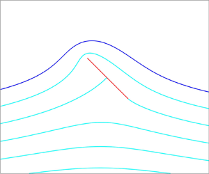
  $\partial D_0$ is unknown a priori but will be determined as part of our solution.

Figure 1. Sketch of the flow domain  $D$ for a free-surface flow past a submerged hydrofoil. Here, $\partial D_0$ denotes the free surface (in blue) while $\partial D_1$ denotes the hydrofoil (red). Also, $z_1=0$ and $z_2=\mathrm {e}^{\mathrm {i}\alpha }$ denote, respectively, the leading and trailing edges of the hydrofoil, so $-\alpha$ gives the angle of attack, and $z_3$ denotes a stagnation point – this lies on the leading face of the hydrofoil.
Without loss of generality, we may normalise the hydrofoil to be of unit length, and fix its leading endpoint to be at the origin. We denote this endpoint by  $z_1$. We denote the trailing endpoint of the foil by $z_2$. Then $z_2=\mathrm {e}^{\mathrm {i}\alpha }$ (so the angle of attack is $-\alpha$), where we consider $\alpha$ over the range $(-{\rm \pi} /2,{\rm \pi} /2)$. The case of a horizontal hydrofoil – i.e. $\alpha =0$ – is trivial (the hydrofoil does not disturb the flow past it), thus we henceforth ignore it (although we will retrieve it later as a limiting case of our results – see § 5.1). We will also not consider a vertical hydrofoil, i.e. $\alpha =\pm {\rm \pi}/2$; this is because our analysis relies on there being a trailing endpoint (we will be imposing the Kutta condition there). (However, we will present the limits of our results as $\alpha \rightarrow \pm {\rm \pi}/2$ – see § 5.2.) For the example sketched in figure 1, $-{\rm \pi} /2<\alpha <0$, so the hydrofoil slopes downwards from its leading endpoint to its trailing endpoint.
We can define a complex potential  $w(z)=\phi (x,y)+\mathrm {i}\,\psi (x,y)$ for the flow, where $\phi (x,y)$ and $\psi (x,y)$ are the associated velocity potential and streamfunction, respectively. $w(z)$ possesses the following properties. It is analytic in the interior of $D$, and $w'(z)=u(x,y)-\mathrm {i}\,v(x,y)$ gives the complex velocity, where here and throughout this paper we use $'$ to indicate the derivative of a function of one variable. It follows from our above assumption of uniform flow at infinity that, to leading order,
 \begin{equation} w(z)\sim Uz\quad\text{as }|z|\rightarrow\infty\ (\text{in }D). \end{equation}
Next, since  $\partial D_0$ and $\partial D_1$ are both streamlines of the flow (of course, strictly speaking, $\partial D_1$ is just part of the streamline that lies along it), $\mathrm {Im}\{w(z)\}$ must be constant along them, i.e.
 \begin{equation} \mathrm{Im}\{w(z)\}=\psi_j\quad\text{for }z\in\partial D_j,\ j=0,1, \end{equation}
for some constants  $\psi _0$ and $\psi _1$. For the same reason, one may deduce that
 \begin{equation} \mathrm{Im}\{\mathrm{e}^{\mathrm{i}\alpha}\,w'(z)\}=0\quad\text{for }z\in \partial D_1. \end{equation}
Furthermore, it follows from Bernoulli's equation and our assumption of an infinite Froude number that
 \begin{equation} \left|w'(z)\right|=U\quad\text{for }z\in \partial D_0. \end{equation}
In addition, one may deduce that for  $z$ local to the leading endpoint $z_1$ ( $=0$) of the hydrofoil, to leading order,
 \begin{equation} w'(z)\sim Az^{{-}1/2}, \end{equation}
for some constant  $A$. Thus the velocity field is singular at $z_1$. To ensure that the velocity field is bounded at the trailing endpoint $z_2$, we impose the Kutta condition there, thus assuming a certain circulation $\varGamma$, say, around the hydrofoil so
 \begin{equation} \oint_{\mathcal{C}} \mathrm{d}w(z)=\varGamma, \end{equation}
where  $\mathcal {C}$ is a simple closed contour that surrounds the hydrofoil, and we integrate around $\mathcal {C}$ in the anticlockwise direction. Finally, one may also deduce that there must be a stagnation point of the flow at some point $z_3$ on the leading face of the hydrofoil. More specifically, one may deduce that for $z$ local to $z_3$, to leading order,
 \begin{equation} w'(z)\sim B (z-z_3), \end{equation}
for some constant  $B$. We assume this to be the only stagnation point of the flow; $z_3$ will not coincide with the leading endpoint $z_1$ except in the case when the hydrofoil is horizontal, which (as stated above) we will ignore.
3. A conformal parametrisation
We will seek  $D$ (which is a doubly connected domain) as the image of a concentric annulus $D_{\zeta }$ in a complex $\zeta$-plane, under a one-to-one conformal map, which we denote by $z(\zeta )$. Such a parametrisation is known to exist by Koebe's extension of Riemann's mapping theorem (e.g. see Goluzin Reference Goluzin1969). Without loss of generality, we may take $D_{\zeta }$ to be the annular domain that is bounded by the circles $C_0$ and $C_1$, which are both centred on the origin and have radii $1$ and $q$, respectively, for some $q$ with $0< q<1$, and assume that $\partial D_j$ is the image under $z(\zeta )$ of $C_j$, for $j=0,1$. Furthermore, we may assume that the point at infinity in the $z$-plane is the image of $\zeta =-\mathrm {i}$, and, more specifically, that for $\zeta$ local to $-\mathrm {i}$, to leading order,
 \begin{equation} z(\zeta)\sim\frac{a}{\zeta+\mathrm{i}}, \end{equation}
for some real constant  $a>0$. Finally, for $j=1,2,3$, we denote the pre-image of $z_j$ by $\zeta _j$, which lies on $C_1$. For a given hydrofoil, having made the assumptions on $z(\zeta )$ that are listed above, we are not at liberty to choose $\zeta _j$, $j=1,2,3$; instead, we must solve for these, as explained below. One may deduce (on purely geometrical grounds) that $z'(\zeta )$ has simple zeros at both $\zeta =\zeta _1$ and $\zeta _2$. An example is sketched in figure 2. Here, $\zeta _3$ lies on the section of $C_1$ that is traversed in passing from $\zeta _1$ to $\zeta _2$ in the anticlockwise direction, which is the case for a hydrofoil that slopes downwards from its leading endpoint to its trailing endpoint. However, our subsequent analysis makes no assumption on the ordering of $\zeta _1$, $\zeta _2$ and $\zeta _3$ around $C_1$.

Figure 2. Sketch of the pre-image domain  $D_{\zeta }$ for our conformal parametrisation of the flow domain $D$ as in figure 1. Here, $D$ is the image of $D_{\zeta }$ under a conformal map $z(\zeta )$.
Now, in terms of  $\zeta$, we have
 \begin{equation} w(z)=W(\zeta),\quad w'(z)=\varOmega(\zeta), \end{equation}
for some functions  $W$, the complex potential in $D_{\zeta }$, and $\varOmega$, the complex velocity mapped to $D_{\zeta }$ . We construct below formulae (in terms of $\zeta$) for $W(\zeta )$, $\varOmega (\zeta )$, and then make use of the fact that (Joukovskii Reference Joukovskii1890; Michell Reference Michell1890)
 \begin{equation} z'(\zeta)=\frac{\mathrm{d}W/\mathrm{d}\zeta}{\mathrm{d}w/\mathrm{d}z}=\frac{W'(\zeta)}{\varOmega(\zeta)}, \end{equation}
to construct a formula for  $z(\zeta )$. A similar construction is used to obtain the hollow vortex solutions in Crowdy & Green (Reference Crowdy and Green2011) and Crowdy et al. (Reference Crowdy, Llewellyn Smith and Freilich2013), where, however, the integration (3.3) is performed numerically, in contrast to the analytical result below.
3.1. Some special functions
We will perform our construction in terms of certain special functions, labelled here as  $P(\zeta,q)$, $K(\zeta,q)$ and $L(\zeta,q)$. We define these and state their relevant properties in this section. We refer the reader to Crowdy (Reference Crowdy2020) for further discussion of these functions, including their connection to more traditionally used elliptic functions (as used, for example, in Gurevitch Reference Gurevitch1965; Semenov & Wu Reference Semenov and Wu2020). The advantage of the functions that we use here is that their singularity and periodicity structures present themselves clearly, although it should be possible to derive similar properties for elliptic functions.
To begin, we define the transformation  $\theta _n(\zeta )=q^{2n}\zeta$ for all $n\in \mathbb {Z}$ (note that $\theta _0(\zeta )=\zeta$ is the identity transformation), and the set $\varTheta =\{\theta _n(\zeta )\mid n\in \mathbb {Z}\}$. Next, we introduce $D_{\zeta }^{-1}$ to denote the reflection of $D_{\zeta }$ in $C_0$, where by reflection in $C_0$ we mean the transformation $\zeta \mapsto 1/\bar {\zeta }$: $D_{\zeta }^{-1}$ is the annular domain bounded by the circles $C_0$ and $C_{-1}$, where the latter denotes the reflection of $C_1$ in $C_0$ and is centred on the origin and of radius $1/q$ (see figure 3). We define $F$ to be the region that consists of the union of $\overline {D_{\zeta }}$ and $D_{\zeta }^{-1}$, where we use the ‘overline’ notation with respect to a domain to denote the domain's closure, i.e.
 \begin{equation} F=\{\zeta:q\leq|\zeta|< q^{{-}1}\}, \end{equation}
so  $F$ does not contain $C_{-1}$. The images of $F$ under all elements of $\varTheta$ are mutually disjoint and cover the whole of the $\zeta$-plane, except for the origin and the point at infinity. $\varTheta$ is in fact an example of a Schottky group (Ford Reference Ford1972; Crowdy Reference Crowdy2020). We refer to $F$ as a fundamental region of $\varTheta$. (The fundamental region of a Schottky group is not unique.)

Figure 3. The annuli appearing in the analysis:  $D_{\zeta }^{-1}$ (light grey) is the reflection of the pre-image domain $D_{\zeta }$ (turquoise) of figure 2 in the unit circle $C_0$ (dotted blue). The union of $\overline {D_{\zeta }}$ and $D_{\zeta }^{-1}$ forms the fundamental region $F$ of (3.4) for the group $\varTheta$. The union of $\bar {F}$ and the reflection of $F$ (dark grey) in the circle $C_1$ (dotted red) forms the fundamental region $\hat {F}$ of (3.13) for the group $\hat {\varTheta }$. The complex velocity $W'(\zeta )$ has double poles (blue crosses) at $\zeta =-\mathrm {i}$ and $-\mathrm {i}q^2$, and simple zeros (blue circles) at $\zeta =\zeta _2$, $-\overline {\zeta _2}$, $1/\overline {\zeta _2}$ and $-1/\zeta _2$. The mapped complex velocity $\varOmega (\zeta )$ has simple poles (red crosses) at $\zeta =\zeta _1$ and $-1/\zeta _2$ (coinciding with a zero of $W'(\zeta )$), and simple zeros (red discs) at $\zeta =1/\overline {\zeta _1}$ and $-\overline {\zeta _2}$ (also coinciding with a zero of $W'(\zeta )$).
Now, the function  $P(\zeta,q)$ is defined for all complex $\zeta$ and (real) $q$ with $0< q<1$, by
 \begin{equation} P(\zeta,q)=(1-\zeta)\prod_{n=1}^{\infty}(1-q^{2n}\zeta)(1-q^{2n}\zeta^{{-}1}). \end{equation}
Up to a normalisation,  $P(\zeta,q)$ is the Schottky–Klein prime function associated with $\varTheta$. One can check that $P(\zeta,q)$ is analytic everywhere in $F$, and is non-zero in $F$ except for a simple zero at $\zeta =1$. Furthermore, one can deduce directly from (3.5) that
 \begin{equation} P(q^2\zeta,q)={-}\zeta^{{-}1}\,P(\zeta,q), \quad P(\zeta^{{-}1},q)={-}\zeta^{{-}1}\,P(\zeta,q). \end{equation}
Relation (3.6a) can be used to continue  $P(\zeta,q)$ to points $\zeta$ outside of $F$. In particular, one can deduce from (3.6a), and the properties of $P(\zeta,q)$ for $\zeta \in F$ noted above, that $P(\zeta,q)$ is analytic everywhere in the $\zeta$-plane except for essential singularities at the origin and the point at infinity, and that it has simple zeros at $\zeta =q^{2n}$ for all $n\in \mathbb {Z}$. Of course, one could also deduce these properties directly from (3.5).
Next, the function  $K(\zeta,q)$ is defined by
 \begin{equation} K(\zeta,q)=\zeta\,\frac{\mathrm{d}}{\mathrm{d}\zeta}\log P(\zeta,q). \end{equation}
It follows from (3.5) that
 \begin{equation} K(\zeta,q)= \frac{1}{\zeta-1}+1 +\sum_{n=1}^{\infty} q^{2n} \left( \frac{1}{\zeta-q^{2n}} -\frac{1}{\zeta^{{-}1}-q^{2n}} \right). \end{equation}
One may check that  $K(\zeta,q)$ is analytic everywhere in $F$ except for a simple pole at $\zeta =1$ with residue $1$. Also, it follows from (3.6) that
 \begin{equation} K(q^2\zeta,q)=K(\zeta,q)-1, \quad K(\zeta^{{-}1},q)=1-K(\zeta,q). \end{equation}
 Finally, the function  $L(\zeta,q)$ is defined by
 \begin{equation} L(\zeta,q)=\zeta\,\frac{\mathrm{d}}{\mathrm{d}\zeta}K(\zeta,q). \end{equation}
It follows from (3.8) that
 \begin{equation} L(\zeta,q)= \frac{-1}{(\zeta-1)^2} -\frac{1}{\zeta-1} -\zeta\sum_{n=1}^{\infty} q^{2n} \left( \frac{1}{(\zeta-q^{2n})^2} +\frac{1}{(1-q^{2n}\zeta)^2} \right). \end{equation}
One may check that  $L(\zeta,q)$ is analytic everywhere in $F$ except for a double pole at $\zeta =1$ with residue $-1$. Also, it follows from (3.9) that
 \begin{equation} L(q^2\zeta,q)=L(\zeta,q), \quad L(\zeta^{{-}1},q)=L(\zeta,q). \end{equation}
 In addition to the above, we will also make use of the functions  $P(\zeta,q^2)$, $K(\zeta,q^2)$ and $L(\zeta,q^2)$. Of course, with $0< q<1$, we also have $0< q^2<1$, so $P(\zeta,q^2)$ is defined by (3.5) simply with $q$ replaced by $q^2$. And $P(\zeta,q^2)$ is (up to a normalisation) the Schottky–Klein prime function associated with $\hat {\varTheta }=\{\theta _{2n}(\zeta )\mid n\in \mathbb {Z}\}$, which is a subgroup of $\varTheta$ and itself a Schottky group (Vasconcelos, Marshall & Crowdy Reference Vasconcelos, Marshall and Crowdy2015). A fundamental region of $\hat {\varTheta }$ is
 \begin{equation} \hat{F}=\{\zeta:q^3<|\zeta|\leq q^{{-}1}\}, \end{equation}
i.e. the region that consists of the union of  $\bar {F}$ and the reflection of $F$ in the circle $C_1$, where reflection in $C_1$ is given by $\zeta \mapsto q^2/\bar {\zeta }$ (see figure 3).
It follows directly from (3.5) that
 \begin{equation} P(\zeta,q)=P(\zeta,q^2)\,P(q^2\zeta,q^2), \end{equation}
and hence from (3.7) and (3.10) that
 \begin{equation} K(\zeta,q)=K(\zeta,q^2)+K(q^2\zeta,q^2), \quad L(\zeta,q)=L(\zeta,q^2)+L(q^2\zeta,q^2). \end{equation}
3.2. Constructing the complex potential  $W(\zeta )=w(z)$
The construction of  $W(\zeta )$ is straightforward as it is simply the complex potential for flow in the annulus $D_{\zeta }$, driven by a dipole at $-\mathrm {i}$ and having circulation $\varGamma$ around $C_1$ with stagnation points at $\zeta _2$ and $\zeta _3$. Since both $D_{\zeta }$ and the dipole flow are right–left symmetric, $\zeta _3=-\overline {\zeta _2}$, as shown in § 3.2.1 below. Figure 4(a) shows contours of $\mathrm {Im}\{W(\zeta )\}$ – i.e. flow streamlines – in $D_{\zeta }$ for a typical solution.

Figure 4. Illustrations of the solution components for a typical solution (namely, that which is illustrated in figure 6(b) below). Here,  $\alpha =-{\rm \pi} /4$ and $y_c=0.3$ (see (3.51)). (a) Contours of $\mathrm {Im}\{W(\zeta )\}$ as given by (3.19), giving the flow streamlines in the pre-image domain $D_{\zeta }$ with a dipole at $\zeta =\mathrm {-i}$ (which corresponds to the point at infinity in $D$), stagnation points symmetrically at $\zeta =\zeta _2$ (the trailing edge in $D$) and $-\overline {\zeta _2}$ (on the leading face in $D$), and tangential flow along $C_0$ (the free surface in $D$) and $C_1$ (the foil). (b) Isotachs, contours of $|\varOmega (\zeta )|$ as given by (3.34), the flow speed mapped to the pre-image domain $D_{\zeta }$, with infinite speed at $\zeta _1$ (the leading edge in $D$), a single stagnation point at $\zeta =-\overline {\zeta _2}$ (on the leading face in $D$), and constant speed along $C_0$ (the free surface in $D$), with no stagnation point at $\zeta =\zeta _2$ (the trailing edge in $D$) where the speed is finite.
It follows from the properties of  $w(z)$ and $z(\zeta )$ noted above that $W(\zeta )$ must be analytic for all $\zeta \in D_{\zeta }$ except that (as follows from (2.1) and (3.1)) for $\zeta$ local to $-\mathrm {i}$, to leading order,
 \begin{equation} W(\zeta)\sim\frac{Ua}{\zeta+\mathrm{i}}. \end{equation}
Also, it follows from (2.2) that
 \begin{equation} \mathrm{Im}\{W(\zeta)\}=\psi_j\quad\text{for }\zeta\in C_j,\ j=0,1. \end{equation}
Furthermore, it follows from (2.6) that
 \begin{equation} \oint_{\hat{\mathcal{C}}} \,\mathrm{d}W(\zeta)=\varGamma, \end{equation}
where we can take  $\hat {\mathcal {C}}$ to be a circle centred on the origin, of some radius $\hat {q}$, where $q<\hat {q}<1$ (so that $\hat {\mathcal {C}}$ lies in the interior of $D_{\zeta }$), and we integrate around $\hat {\mathcal {C}}$ in the anticlockwise direction. Recall that $\varGamma$ is still to be determined. We propose that
 \begin{equation} W(\zeta) = Ua\mathrm{i}\,K(\mathrm{i}\zeta,q) -\frac{\mathrm{i}\varGamma}{2{\rm \pi}}\log\zeta. \end{equation}
One can verify that  $W(\zeta )$ as stated by (3.19) possesses the properties stated above, as follows. First, it follows from the properties of $K(\zeta,q)$, that $W(\zeta )$ as given by (3.19) is analytic for all $\zeta \in D_{\zeta }$ except for a simple pole with residue $Ua$ at $\zeta =-\mathrm {i}$, as required by (3.16). It is also evident that this form for $W(\zeta )$ satisfies (3.18). Finally, to check the boundary conditions (3.17), it is helpful to first note that
 \begin{equation}
\mathrm{Re}\{K(\mathrm{i}\zeta,q)\}=\tfrac{1}{2}\left(K(\mathrm{i}\zeta,q)+K(1/(\mathrm{i}\zeta),q)\right)=\tfrac{1}{2}\quad\text{for
}\zeta\in C_0, \end{equation}
\begin{equation}
\mathrm{Re}\{K(\mathrm{i}\zeta,q)\}=\tfrac{1}{2}\left(K(\mathrm{i}\zeta,q)+K(1/(\mathrm{i}\zeta),q)\right)=\tfrac{1}{2}\quad\text{for
}\zeta\in C_0, \end{equation}
where the first equality follows from the fact that for  $\zeta \in C_0$, $\bar {\zeta }=1/\zeta$, and the second follows from (3.9b). Similarly,
 \begin{equation} \mathrm{Re}\{K(\mathrm{i}\zeta,q)\}=\tfrac{1}{2}(K(\mathrm{i}\zeta,q)+K(q^2/(\mathrm{i}\zeta),q))=0\quad\text{for }\zeta\in C_1, \end{equation}
where now the first equality follows from the fact that for  $\zeta \in C_1$, $\bar {\zeta }=q^2/\zeta$, and the second follows by using both equations in (3.9). Then one may deduce that (3.17) holds (with $\psi _0=Ua/2$ and $\psi _1=-(\varGamma /(2{\rm \pi} ))\ln q$). This completes our verification of (3.19). Similar arguments to those below for $\varOmega (\zeta )$ show that $W(\zeta )$ is unique.
Differentiating (3.19) gives
 \begin{equation} W'(\zeta) = \frac{1}{\zeta} \left( Ua\mathrm{i}\,L(\mathrm{i}\zeta,q)-\frac{\mathrm{i}\varGamma}{2{\rm \pi}} \right). \end{equation}
Now, in order to impose the Kutta condition at the trailing endpoint  $z_2$ of the hydrofoil, we must choose $\varGamma$ such that $W'(\zeta _2)=0$, giving
 \begin{equation} \varGamma=2{\rm \pi} Ua\,L(\mathrm{i}\zeta_2,q). \end{equation}
(Note that it follows from (3.24) that  $L(\mathrm {i}\zeta _2,q)$ is real.)
3.2.1. Properties of $W'(\zeta )$, the complex velocity in $D_\zeta$


We now note some properties of  $W'(\zeta )$ that will be useful later. First, $W'(-\overline {\zeta _2})=0$. This follows from (3.22) using the fact that $W'(\zeta _2)=0$ and
 \begin{equation} L(-\mathrm{i}\overline{\zeta_2},q)=L(q^2/(\mathrm{i}\zeta_2),q)=L(\mathrm{i}\zeta_2,q), \end{equation}
where the second equality follows by using both equations in (3.12). We will henceforth assume that  $-\overline {\zeta _2}\neq \zeta _2$, or equivalently, that $\zeta _2\neq \pm \mathrm {i}q$ (although, in § 5.2, we will consider the limit of our results as $\zeta _2\rightarrow \pm \mathrm {i}q$, whilst $\zeta _1\rightarrow \mp \mathrm {i}q$, respectively). We now claim that the zeros of $W'(\zeta )$ at $\zeta =\zeta _2$ and $-\overline {\zeta _2}$ are the only zeros of $W'(\zeta )$ in $F$, and are simple zeros. To demonstrate this, note that it follows from (3.22) and (3.12a) that
 \begin{equation} W'(q^2\zeta)=\frac{1}{q^2}\,W'(\zeta). \end{equation}
Thus
 \begin{equation} \mathrm{d}\log W'(q^2\zeta)=\mathrm{d}\log W'(\zeta). \end{equation}
It then follows from (3.26) and an application of the argument principle (Ahlfors Reference Ahlfors1979, § 5.2) that  $W'(\zeta )$ has the same number of poles as zeros in $F$, where these are both counted according to their multiplicities. (Here, $\zeta _2$ and $-\overline {\zeta _2}$ lie on the boundary of $F$, but by standard arguments one can adapt the argument principle to take account of this.) But it follows from (3.22) and the properties of $L(\zeta,q)$ that $W'(\zeta )$ has a double pole at $\zeta =-\mathrm {i}$ and no other singularities in $F$. Thus, as claimed, the zeros of $W'(\zeta )$ at $\zeta =\zeta _2$ and $-\overline {\zeta _2}$ must be the only zeros of $W'(\zeta )$ in $F$, and must be simple zeros. It also then follows that
 \begin{equation} \zeta_3={-}\overline{\zeta_2}. \end{equation}
 Finally, one may also deduce that  $W'(\zeta )$ is analytic for all $\zeta \in \hat {F}$ except for double poles at $\zeta =-\mathrm {i}$ and $-\mathrm {i}q^2$, and that the only zeros of $W'(\zeta )$ in $\hat {F}$ are simple zeros at $\zeta =\zeta _2$, $-\overline {\zeta _2}$, $1/\overline {\zeta _2}$ and $-1/\zeta _2$ – see figure 3. ( $W'(\zeta )$ also has zeros at $\zeta =q^2\zeta _2$ and $-q^2\overline {\zeta _2}$, but both of these points have modulus $q^3$ and so are not contained in $\hat {F}$.)
3.3. Constructing the mapped complex velocity $\varOmega (\zeta )=w'(z)$
It follows from the properties of  $w'(z)$ and $z(\zeta )$ stated above that $\varOmega (\zeta )$ must be analytic for all $\zeta \in D_{\zeta }$ except for a simple pole at $\zeta =\zeta _1$ (as follows from (2.5) and the fact that $z'(\zeta )$ has a simple zero at $\zeta _1$). Furthermore, $\varOmega (\zeta )$ must be non-zero for all $\zeta$ in the closure of $D_{\zeta }$ except for a simple zero at $\zeta =-\overline {\zeta _2}$ (as follows from (2.7), recalling (3.27)). Note that $\varOmega (\zeta )$ is non-zero at $\zeta =\zeta _2$ – i.e. $w'(z)$ is non-zero at the trailing endpoint $z_2$ of the hydrofoil – because $W'(\zeta )$ and $z'(\zeta )$ both have simple zeros at $\zeta =\zeta _2$ (and $\varOmega (\zeta )=W'(\zeta )/z'(\zeta )$). In addition, it follows from (2.3) and (2.4) that
 \begin{equation} \left|\varOmega(\zeta)\right|=U\text{ for }\zeta\in C_0, \quad \mathrm{Im}\{\mathrm{e}^{\mathrm{i}\alpha}\,\varOmega(\zeta)\}=0\text{ for }\zeta\in C_1, \end{equation}
and from (2.1) that
 \begin{equation} \varOmega(-\mathrm{i}) = U. \end{equation}
Figure 4(b) illustrates the mapped flow speed  $|\varOmega (\zeta )|$ in $D_{\zeta }$ for a typical solution.
It follows from (3.28a) that for  $\zeta \in C_0$, since $\bar {\zeta }=1/\zeta$,
 \begin{equation} \varOmega(\zeta)=\frac{U^2}{\bar{\varOmega}(1/\zeta)}, \end{equation}
where we define  $\bar {\varOmega }(\zeta )=\overline {\varOmega (\bar {\zeta })}$. However, it follows from the properties of $\varOmega (\zeta )$ that $1/\bar {\varOmega }(1/\zeta )$ is analytic for all $\zeta \in D_{\zeta }^{-1}$ except for a simple pole at $\zeta =-1/\zeta _2$, and also non-zero for all $\zeta$ in the closure of $D_{\zeta }^{-1}$ except for a simple zero at $\zeta =1/\overline {\zeta _1}$. It then follows by analytic continuation that (3.30) must in fact hold for all $\zeta$ in the closure of $F$, and that $\varOmega (\zeta )$ is analytic for all $\zeta \in F$ except for simple poles at $\zeta =\zeta _1$ and $-1/\zeta _2$. Furthermore, the only zeros of $\varOmega (\zeta )$ in $F$ are simple zeros at $\zeta =-\overline {\zeta _2}$ and $1/\overline {\zeta _1}$.
Next, one may deduce from (3.28b) that for  $\zeta \in C_1$, since $\bar {\zeta }=q^2/\zeta$,
 \begin{equation} \varOmega(\zeta)=\mathrm{e}^{{-}2\mathrm{i}\alpha}\,\bar{\varOmega}(q^2/\zeta). \end{equation}
Then, by arguments similar to those just stated after (3.30), it follows that (3.31) must in fact hold for all  $\zeta$ in the closure of $\hat {F}$. But furthermore, one may deduce that $\varOmega (\zeta )$ is analytic for all $\zeta \in \hat {F}$ except for simple poles at $\zeta =\zeta _1$ and $-1/\zeta _2$, and that the only zeros of $\varOmega (\zeta )$ in $\hat {F}$ are simple zeros at $\zeta =-\overline {\zeta _2}$ and $1/\overline {\zeta _1}$ – see figure 3.
Now note that by repeated analytic continuation, one may show that (3.30) and (3.31) in fact hold for all  $\zeta$, except at $0$ and infinity. Combining these two relations gives
 \begin{equation} \varOmega(q^2\zeta)=\frac{\mathrm{e}^{{-}2\mathrm{i}\alpha}\,U^2}{\varOmega(\zeta)}, \end{equation}
hence
 \begin{equation} \varOmega(q^4\zeta)=\varOmega(\zeta), \end{equation}
from which one may deduce that  $\varOmega (\zeta )$ is automorphic with respect to the group $\hat {\varTheta }$. The property (3.33), together with the properties of $\varOmega (\zeta )$ for $\zeta$ in the fundamental region $\hat {F}$ of $\hat {\varTheta }$ that are stated just after (3.31), along with the normalisation (3.29), are enough to identify $\varOmega (\zeta )$ uniquely. To check this, consider the ratio of $\varOmega (\zeta )$ and any other function that has these properties. This ratio must be analytic everywhere in $\hat {F}$ (all poles of the numerator are cancelled by the same poles of the denominator; likewise all zeros of the denominator are cancelled by the same zeros of the numerator), and also automorphic with respect to $\hat {\varTheta }$. It then follows from the extended form of Liouville's theorem for automorphic functions (e.g. see Ford Reference Ford1972), that this ratio must equal a constant. But it follows from the normalisation on $\varOmega (\zeta )$ that is imposed by (3.29) that this constant must equal $1$. We thus seek to construct a function with these properties. One could construct this as a ratio of products of $P$ functions. However, it will be more convenient later – in particular, we will wish to differentiate $\varOmega (\zeta )$ (with respect to $\zeta$) – to instead construct it as a sum of the form
 \begin{equation} \varOmega(\zeta) = \alpha_1\,K(\zeta/\zeta_1,q^2) +\alpha_2\,K(-\zeta_2\zeta,q^2) +\alpha_0, \end{equation}
for some (unique) constants  $\alpha _0$, $\alpha _1$ and $\alpha _2$, which we will determine in due course. We highlight the fact that the second argument of the $K$ functions that appear in (3.34) is $q^2$, not $q$.
$q$.
One may verify (3.34) as follows. First, one may check from the properties of  $K(\zeta,q)$ that for all values of $\alpha _0$, $\alpha _1$ and $\alpha _2$, the function on the right-hand side of (3.34) is analytic for all $\zeta \in \hat {F}$ except for simple poles at $\zeta =\zeta _1$ and $-1/\zeta _2$, as required. However, in order for it to satisfy (3.33), it follows from (3.9a) that
 \begin{equation} \alpha_1+\alpha_2=0. \end{equation}
Next, in order that  $\varOmega (-\overline {\zeta _2})=0$, it follows – using the fact that $K(q^2,q^2)=0$ (which one may deduce by using both equations in (3.9) to show that $K(q^2,q^2)=-K(q^2,q^2)$) – that also
 \begin{equation} \alpha_1\,K(-\overline{\zeta_2}/\zeta_1,q^2)+\alpha_0=0. \end{equation}
Note that we will assume that  $\zeta _1\neq -\overline {\zeta _2}$, as otherwise $K(-\overline {\zeta _2}/\zeta _1,q^2)$ is unbounded and – as will be shown in § 5.1 – the hydrofoil is horizontal.
Next, one could also write down a relation between  $\alpha _0$, $\alpha _1$ and $\alpha _2$ by imposing on (3.34) the condition that $\varOmega (1/\overline {\zeta _1})=0$. However, one can show that this relation can be retrieved from (3.35) and (3.36) (using the fact that $\mathrm {Re}\{K(\zeta,q^2)\}=1/2$ for all $\zeta \in C_0$ – cf. (3.20)). Finally, then, it follows from (3.29) that
 \begin{equation} \alpha_1\,K(-\mathrm{i}/\zeta_1,q^2) +\alpha_2\,K(\mathrm{i}\zeta_2,q^2) +\alpha_0=U. \end{equation}
Combining (3.35)–(3.37), and also making use of (3.9b), one arrives at
 \begin{align}
\alpha_1=\frac{-U}{K(\mathrm{i}\zeta_1,q^2)+K(\mathrm{i}\zeta_2,q^2)-K(-\zeta_1/\overline{\zeta_2},q^2)},
\enspace \alpha_2={-}\alpha_1, \enspace
\alpha_0={-}K(-\overline{\zeta_2}/\zeta_1,q^2)\,\alpha_1.
\end{align}
\begin{align}
\alpha_1=\frac{-U}{K(\mathrm{i}\zeta_1,q^2)+K(\mathrm{i}\zeta_2,q^2)-K(-\zeta_1/\overline{\zeta_2},q^2)},
\enspace \alpha_2={-}\alpha_1, \enspace
\alpha_0={-}K(-\overline{\zeta_2}/\zeta_1,q^2)\,\alpha_1.
\end{align}
This also completes our check on (3.34).
3.4. Completing the solution: constructing the mapping $z(\zeta )$

We now introduce the function
 \begin{equation} H(\zeta)=\zeta\,z'(\zeta), \end{equation}
which may be determined as follows. First, it follows from (3.3) that
 \begin{equation} H(\zeta)=\zeta\,\frac{W'(\zeta)}{\varOmega(\zeta)}. \end{equation}
Then it follows from (3.25) and (3.33) that
 \begin{equation} H(q^4\zeta)=H(\zeta). \end{equation}
Hence  $H(\zeta )$ is automorphic with respect to $\hat {\varTheta }$. Furthermore, one can check from the properties of $W'(\zeta )$ and $\varOmega (\zeta )$ identified in §§ 3.2 and 3.3 that $H(\zeta )$ is analytic everywhere in $\hat {F}$ except for a simple pole at $\zeta =1/\overline {\zeta _1}$ and double poles at $\zeta =-\mathrm {i}$ and $-\mathrm {i}q^2$. These properties of $H(\zeta )$, along with its residues at the aforementioned poles and the coefficients of $(\zeta +\mathrm {i})^{-2}$ and $(\zeta +\mathrm {i}q^2)^{-2}$ in the Laurent series expansions of it about $\zeta =-\mathrm {i}$ and $-\mathrm {i}q^2$, respectively, identify $H(\zeta )$ uniquely, up to an additive constant. This follows by arguments similar to those that we have already applied to $\varOmega (\zeta )$ (see the paragraph just after (3.33)), although one should now consider the difference of $H(\zeta )$ and any other function with these properties; this difference must be analytic everywhere in $\hat {F}$, and automorphic with respect to $\hat {\varTheta }$, and so must equal a constant. It then follows from the properties of $K(\zeta,q)$ and $L(\zeta,q)$ that we can write
 \begin{align} H(\zeta)={}&\beta_1\,K(\overline{\zeta_1}\zeta,q^2) +\beta_2\,K(\mathrm{i}\zeta,q^2) +\beta_3\,K(\mathrm{i}q^2\zeta,q^2)\nonumber\\ &{}+\beta_4\,L(\mathrm{i}\zeta,q^2) +\beta_5\,L(\mathrm{i}q^2\zeta,q^2) +\beta_0, \end{align}
for some unique constants  $\beta _0,\ldots,\beta _5$. We determine these constants in Appendix A.
Now note that, evidently, as follows from (3.39), dividing the right-hand side of (3.42) by  $\zeta$ provides an expression for $z'(\zeta )$. Recalling (3.7) and (3.10), it is straightforward to integrate this expression to find
 \begin{align} z(\zeta)={}&\beta_1 \log P(\overline{\zeta_1}\zeta,q^2) +\beta_2 \log P(\mathrm{i}\zeta,q^2) +\beta_3 \log P(\mathrm{i}q^2\zeta,q^2)\nonumber\\ &{}+\beta_4\,K(\mathrm{i}\zeta,q^2) +\beta_5\,K(\mathrm{i}q^2\zeta,q^2) +c, \end{align}
where  $c$ is an additional constant. One might expect to see the term $\beta _0\log \zeta$ on the right-hand side of (3.43). However, we can omit this for the following reason. Of course, our map $z(\zeta )$ must be single-valued in $D_{\zeta }$; one can check that the form on the right-hand side of (3.43) is indeed so, as follows. First, note that it is straightforward to rewrite (3.5) as
 \begin{equation} P(\zeta,q)= \kappa(q)\,(\zeta-1)\prod_{n=1}^{\infty}(\zeta^{{-}1}(\zeta-q^{2n})(\zeta-q^{{-}2n})), \end{equation}
where  $\kappa (q)$ is independent of $\zeta$ (in fact, $\kappa (q)=-\prod _{n=1}^{\infty }(-q^{2n})$). Then it is evident that the change in $\log P(\zeta,q)$ after $\zeta$ completes a circuit around a circle that is centred on the origin and of radius $\rho$, say, in the anticlockwise direction, is equal to $0$ if $q^2<\rho <1$ (since for each $n\geq 1$, the change due to the logarithmic singularity at $\zeta =q^{2n}$ is cancelled by that due to a logarithmic singularity of opposite strength at the origin), but equal to $2{\rm \pi} \mathrm {i}$ if $1<\rho < q^{-2}$, and so on. For $\zeta \in D_{\zeta }$, we have $q<|\zeta |<1$, and hence $q^4<|\overline {\zeta _1}\zeta |, |\mathrm {i}\zeta |, |\mathrm {i}q^2\zeta |<1$. It then follows that the terms $\log P(\overline {\zeta _1}\zeta,q^2)$, $\log P(\mathrm {i}\zeta,q^2)$ and $\log P(\mathrm {i}q^2\zeta,q^2)$ that appear in (3.43) are all single-valued in $D_{\zeta }$. And $K(\mathrm {i}\zeta,q^2)$ and $K(\mathrm {i}q^2\zeta,q^2)$ are also both single-valued in $D_{\zeta }$. However, $\beta _0\log \zeta$ is not single-valued in $D_{\zeta }$. Hence
 \begin{equation} \beta_0=0, \end{equation}
so the integrated form for our map  $z(\zeta )$ is given by (3.43) and is single-valued in $D_{\zeta }$. Condition (3.45) places a constraint on our mapping parameters, as we discuss further in the next subsection.
3.5. Specifying parameter values
Our parametrisation depends on the following parameters:  $q$,
$q$,  $\arg \{\zeta _1\}$, $\arg \{\zeta _2\}$, $a$ (which, recall, is real and positive) and $c$ (which is complex). Trivially, for any values of $q$,
$q$,  $\arg \{\zeta _1\}$ and $\arg \{\zeta _2\}$, we can fix $c$ and $a$ to ensure that $z_1=0$ and the length of the hydrofoil is $1$; more specifically, it follows from (3.43) that we should take
 \begin{align}
c&={-}(\beta_1 \log P(q^2,q^2) +\beta_2 \log
P(\mathrm{i}\zeta_1,q^2) +\beta_3 \log
P(\mathrm{i}q^2\zeta_1,q^2)\nonumber\\&\qquad\ +\beta_4\,K(\mathrm{i}\zeta_1,q^2)
+\beta_5\,K(\mathrm{i}q^2\zeta_1,q^2)) \end{align}
\begin{align}
c&={-}(\beta_1 \log P(q^2,q^2) +\beta_2 \log
P(\mathrm{i}\zeta_1,q^2) +\beta_3 \log
P(\mathrm{i}q^2\zeta_1,q^2)\nonumber\\&\qquad\ +\beta_4\,K(\mathrm{i}\zeta_1,q^2)
+\beta_5\,K(\mathrm{i}q^2\zeta_1,q^2)) \end{align}
with
 \begin{align} a=
\Bigl|&\hat{\beta}_1 \log
P(\overline{\zeta_1}\zeta_2,q^2) +\hat{\beta}_2 \log
P(\mathrm{i}\zeta_2,q^2) +\hat{\beta}_3 \log
P(\mathrm{i}q^2\zeta_2,q^2)\nonumber\\ &{}+\hat{\beta}_4\,K(\mathrm{i}\zeta_2,q^2)
+\hat{\beta}_5\,K(\mathrm{i}q^2\zeta_2,q^2) +\hat{c}
\Bigr|^{{-}1}, \end{align}
\begin{align} a=
\Bigl|&\hat{\beta}_1 \log
P(\overline{\zeta_1}\zeta_2,q^2) +\hat{\beta}_2 \log
P(\mathrm{i}\zeta_2,q^2) +\hat{\beta}_3 \log
P(\mathrm{i}q^2\zeta_2,q^2)\nonumber\\ &{}+\hat{\beta}_4\,K(\mathrm{i}\zeta_2,q^2)
+\hat{\beta}_5\,K(\mathrm{i}q^2\zeta_2,q^2) +\hat{c}
\Bigr|^{{-}1}, \end{align}
where here we use  $\hat {\beta }_j$ to denote $\beta _j/a$ for $j=1,\ldots,5$, and $\hat {c}$ to denote $c/a$. (It is evident that one may factor out $a$ from our expressions (A11), (A7), (A9), (A1) and (A5) for $\beta _1,\ldots,\beta _5$, and hence also from our expression (3.46) for $c$.) Next, in order to fix $\arg \{z_2\}=\alpha$, one could use the condition that one obtains by simply setting $\zeta =\zeta _2$ on the right-hand side of (3.43) and then requiring that the argument of this equals $\alpha$. However, a simpler condition is given by (3.49) below. One may deduce this by noting that it follows from (3.31) and (3.34) (along with both equations in (3.9)) that
 \begin{equation} \frac{\overline{\alpha_1}}{\alpha_1}={-}\mathrm{e}^{2\mathrm{i}\alpha}, \end{equation}
and hence from (3.38a) (and both equations in (3.9) again) that
 \begin{equation} \frac{K(\mathrm{i}\zeta_1,q^2)+K(\mathrm{i}\zeta_2,q^2)-K(-\zeta_1/\overline{\zeta_2},q^2)} {K(\mathrm{i}q^2\zeta_1,q^2)+K(\mathrm{i}q^2\zeta_2,q^2)+K(-\overline{\zeta_2}/\zeta_1,q^2)} =\mathrm{e}^{2\mathrm{i}\alpha}. \end{equation}
Finally, in addition to the above, we must also impose the single-valuedness condition (3.45) with  $\beta _0$ as given by (A12), which one can show is equivalent to
 \begin{align} L(\mathrm{i}\zeta_1,q^2)+\mathrm{e}^{2\mathrm{i}\alpha}\,L(\mathrm{i}q^2\zeta_1,q^2) - \frac{\left(L(\mathrm{i}\zeta_1,q^2)-L(\mathrm{i}\zeta_2,q^2)\right)\left( K(\mathrm{i}\zeta_1,q^2)-\mathrm{e}^{2\mathrm{i}\alpha}\,K(\mathrm{i}q^2\zeta_1,q^2) \right)} {K(\mathrm{i}\zeta_1,q^2)+K(\mathrm{i}\zeta_2,q^2)-K(-\zeta_1/\overline{\zeta_2},q^2)} =0. \end{align}
Equations (3.49) and (3.50) fix two of the remaining three parameters  $\arg \{\zeta _1\}$, $\arg \{\zeta _2\}$ and $q$. This leaves one remaining free parameter. As is borne out by the examples presented in § 6, one could interpret this remaining parameter as corresponding in some sense to the depth of the hydrofoil below the free surface. As a measure of this depth, we will adopt the following. Recall that we fix the leading and trailing endpoints of the hydrofoil to be at the origin and $\mathrm {e}^{\mathrm {i}\alpha }$, respectively. We now seek some convenient reference level for the $y$-coordinate of points on the free surface. As we show next in § 3.6, in general, $y$ does not tend to a constant along the free surface as $|x|\rightarrow \infty$. However (as is the case for the examples that we present in § 6), it appears that there is a single (finite) point, say $z_c$, on the free surface at which $\mathrm {d} y/\mathrm {d} x=0$; there is a peak of the free surface at $z_c$ when the leading endpoint of the hydrofoil is above its trailing endpoint – i.e. when $\alpha <0$ – and a trough at $z_c$ when $\alpha >0$. Fixing $\mathrm {Im}\{z_c\}=y_c$, say, then essentially fixes the depth of the hydrofoil. This places the following additional condition on our mapping parameters. Of course, $z_c=z(\zeta _c)$ for some $\zeta _c$ on $C_0$ at which $\mathrm {Im}\{\mathrm {d}z(\zeta )/\mathrm {d}\theta \}=0$, where here we use $\theta$ to denote the angular polar coordinate of $\zeta$. Hence (recalling (3.39)) one may deduce that
 \begin{equation} \mathrm{Im}\{z(\zeta_c)\}=y_c \end{equation}
and
 \begin{equation} \mathrm{Re}\{H(\zeta_c)\}=0. \end{equation}
3.6. Limit as $|x|\rightarrow \infty$

To conclude this section, we determine the limiting shape of the free surface as  $|x|\rightarrow \infty$. To do so, we consider the limit of $z(\zeta )$ as given by (3.43) as $\zeta \rightarrow -\mathrm {i}$ along $C_0$. Equivalently, we may take $\zeta =\mathrm {e}^{\mathrm {i}((-{\rm \pi} /2)+\epsilon )}$ and consider the limit of $z(\zeta )$ as $\epsilon \rightarrow 0^{\pm }$. In this limit, the only terms in (3.43) that become singular are $\log P(\mathrm {i}\zeta,q^2)$ and $K(\mathrm {i}\zeta,q^2)$; recalling (3.5) and (3.8) (and using series expansions for $\exp$ and $\log$), one finds that
 \begin{equation} \log P(\mathrm{i}\zeta,q^2)\sim\ln|\epsilon|+O(1),\quad K(\mathrm{i}\zeta,q^2)\sim\frac{\mp\mathrm{i}}{|\epsilon|}+O(1). \end{equation}
Hence, recalling (A1), it follows from (3.43) that in this limit, assuming that  $\beta _2$ and $a$ are of the order of $1$,
$1$,
 \begin{equation} z(\zeta)\sim\beta_2\ln|\epsilon|\pm\frac{a}{|\epsilon|}+O(1). \end{equation}
But, as shown in Appendix A (see its final paragraph),  $\beta _2$ is purely imaginary. It then follows from (3.54) that as $|x|\rightarrow \infty$, the free surface tends to the curve given by
 \begin{equation} y(x)={-}\mathrm{Im}\{\beta_2\}\ln|x|. \end{equation}
Thus the  $y$-coordinate of points on the free surface tends to infinity as $|x|\rightarrow \infty$. SW20 observe the same limiting behaviour for the free surface for flow past a submerged circular cylinder without gravity – see their equation (3.8). The sole exception to this appears to be for $\alpha <0$ in the limit when the depth of the hydrofoil below the free surface tends to zero, as in figure 5. Equally, (4.9) and (4.10) show that the lift coefficient $C_L$ is simply a multiple of $\mathrm {Im}\{\beta _2\}$, and figure 7(a) shows that $C_L\to 0$ as $y_c\to 0$ for $\alpha =-{\rm \pi} /4$.

Figure 5. Free surface profiles (blue) for flow past a hydrofoil (red) for various angles of attack  $-\alpha$ and leading-edge submergence $y_c$: (a) $\alpha =-{\rm \pi} /4$, $y_c=0.01, 0.05$ and $0.1, 0.2, 0.3,\dots$; and (b) $\alpha ={\rm \pi} /3$, $y_c=0.28, 0.8$ and $1.2, 1.4, 1.6, \ldots$. Lengths here and in subsequent figures are normalised on the length of the foil.
4. The force on the hydrofoil
We denote the (vector) force that is exerted by the fluid on the hydrofoil by  $\boldsymbol {F}$, and the components of this force in the $x$- and $y$-directions by $F_x$ and $F_y$, respectively. From Blasius's theorem, we have
 \begin{equation} F_x-\mathrm{i}F_y =\frac{\mathrm{i}\rho}{2} \oint_{\mathcal{C}} \left( w'(z) \right)^2 \,\mathrm{d}z, \end{equation}
where, as in (2.6),  $\mathcal {C}$ is a simple closed contour that surrounds the hydrofoil, and we integrate around $\mathcal {C}$ in the anticlockwise direction, and $\rho$ is the density of the fluid. Using (3.3), we can write the integral in (4.1) in terms of $\zeta$ as
 \begin{equation} F_x-\mathrm{i}F_y =\frac{\mathrm{i}\rho}{2} \oint_{\hat{\mathcal{C}}} W'(\zeta)\,\varOmega(\zeta)\, \mathrm{d}\zeta, \end{equation}
where we can take  $\hat {\mathcal {C}}$ to be as in (3.18), and we integrate around it in the anticlockwise direction. We can in fact compute the integral in (4.2) analytically, as follows.
First, let us introduce the function
 \begin{equation} \eta(\zeta)=\zeta\,W'(\zeta)\,\varOmega(\zeta). \end{equation}
One may determine  $\eta (\zeta )$ by following an approach similar to that which we used to determine the function $H(\zeta )$ in § 3.4 (and $\varOmega (\zeta )$ previously). First, it follows from (3.25) and (3.33) that
 \begin{equation} \eta(q^4\zeta)=\eta(\zeta), \end{equation}
so  $\eta (\zeta )$ is automorphic with respect to $\hat {\varTheta }$. Next, one can check from the properties of $W'(\zeta )$ and $\varOmega (\zeta )$ that $\eta (\zeta )$ is analytic everywhere in $\hat {F}$ except for a simple pole at $\zeta =\zeta _1$, and double poles at $\zeta =-\mathrm {i}$ and $-\mathrm {i}q^2$. It then follows that we can write
 \begin{align} \eta(\zeta)= \gamma_1\,K(\zeta/\zeta_1,q^2) +\gamma_2\,K(\mathrm{i}\zeta,q^2) +\gamma_3\, K(\mathrm{i}q^2\zeta,q^2) +\gamma_4\,L(\mathrm{i}\zeta,q^2) +\gamma_5\,L(\mathrm{i}q^2\zeta,q^2) +\gamma_0, \end{align}
for some unique constants  $\gamma _0,\ldots,\gamma _5$. Before attempting to determine these, note that, evidently, we can write (4.2) as
 \begin{equation} F_x-\mathrm{i}F_y =\frac{\mathrm{i}\rho}{2} \oint_{\hat{\mathcal{C}}} \frac{\eta(\zeta)}{\zeta}\, \mathrm{d}\zeta. \end{equation}
But then, by arguments similar to those that we used when integrating  $H(\zeta )/\zeta$ (with $H(\zeta )$ given by (3.42)) in § 3.4 (in particular, see text between (3.43) and (3.45)), one can compute the integral of $\eta (\zeta )/\zeta$ that appears in (4.6) (with $\eta (\zeta )$ given by (4.5)) analytically; one finds simply that
 \begin{equation} \oint_{\hat{\mathcal{C}}} \frac{\eta(\zeta)}{\zeta}\, \mathrm{d}\zeta=2{\rm \pi}\mathrm{i}(\gamma_0+\gamma_1). \end{equation}
Thus, in order to determine  $\boldsymbol {F}$, it remains only to determine the sum $\gamma _0+\gamma _1$. We do so in Appendix B – see in particular (B3) – showing that it is simply a multiple of $\beta _2$. It then follows from (4.6), (4.7) and (B3) that
 \begin{equation} F_x-\mathrm{i}F_y={-}{\rm \pi}\rho U^2\beta_2. \end{equation}
Appendix A shows  $\beta _2$ to be purely imaginary. It then follows from (4.8) that $\boldsymbol {F}$ has only a vertical component (i.e. $F_x=0$), given by
 \begin{equation} F_y={\rm \pi}\rho U^2\,\mathrm{Im}\{\beta_2\}. \end{equation}
The lift coefficient  $C_L$ for a two-dimensional lifting surface is defined as the force (per unit width in the spanwise direction) in the direction perpendicular to the oncoming flow at infinity, scaled on $\tfrac {1}{2} \rho U^2 \ell$, where $\ell$ is the length of the chord of the lifting surface. Here, the normalisation gives $\ell =1$, so
 \begin{equation} C_L = 2 F_y / \rho U^2, \end{equation}
with  $F_y$ given by (4.9) (and $\beta _2$ by (A7)). Section 6 discusses the behaviour of $C_L$ as a function of $\alpha$ and $y_c$.
5. Limiting cases
5.1. A horizontal hydrofoil
In deriving our parametrisation, we have assumed that  $\zeta _1\neq -\overline {\zeta _2}$ (see just after (3.36)), i.e. that $\zeta _1$ and $\zeta _2$ are not reflections of one another in the imaginary $\zeta$-axis. However, let us now consider the limit of our results as $-\zeta _1/\overline {\zeta _2}\rightarrow 1$. First, in this limit, it is evident from (3.38a,b) and (3.37) that (since $K(-\zeta _1/\overline {\zeta _2},q^2)$ becomes unbounded) $\alpha _1=\alpha _2=0$ and $\alpha _0=U$, and hence, as follows from (3.34), $\varOmega (\zeta )=U$ for all $\zeta$. Thus $w'(z)=U$ for all $z$. It follows that in this case the hydrofoil must be horizontal. Indeed, it follows that in this case our expressions for the constants $\beta _1,\ldots,\beta _5$ – see Appendix A – reduce to
 \begin{equation} \beta_1=\beta_2=\beta_3=0,\quad\beta_4=\beta_5=a\mathrm{i}, \end{equation}
and hence our expression (3.43) for  $z(\zeta )$ reduces to
 \begin{equation} z(\zeta)=a\mathrm{i}\,K(\mathrm{i}\zeta,q)+c, \end{equation}
where we have made use of (3.15a). And one can check by using the properties of  $K(\zeta,q)$ that $z(\zeta )$ as given by (5.2) maps $C_1$ onto a horizontal line segment of finite length. Furthermore, one can also check that it maps $C_0$ onto a horizontal line that extends to infinity in both directions – this is the free surface in this case. We also mention that in this case, it follows from (5.1a,b) (and (3.15b)) that $\beta _0$ – as given by (A12) – reduces to
 \begin{equation} \beta_0 ={-}a\mathrm{i}\,L(\mathrm{i}\zeta_1,q). \end{equation}
And since  $z'(\zeta _1)=0$, it follows from (5.2) (and (3.10)) that $L(\mathrm {i}\zeta _1,q)=0$, and hence from (5.3) that $\beta _0=0$. Thus in this case, the single-valuedness condition (3.45) is satisfied automatically. For a similar reason, it follows from (3.23) that the circulation $\varGamma$ around the hydrofoil in this case is also $0$. Furthermore, it follows from (4.9) (and the fact that now $\beta _2=0$) that in this case, the fluid exerts no force on the hydrofoil.
5.2. Near-vertical hydrofoils
We have also thus far assumed that  $-\overline {\zeta _2}\neq \zeta _2$, or equivalently, that $\zeta _2\neq \pm \mathrm {i}q$ (see just after (3.24)). Let us now consider the limits of our results as $\zeta _2\rightarrow \pm \mathrm {i}q$ whilst $\zeta _1\rightarrow \mp \mathrm {i}q$, respectively. First, in both of these limits, it is evident from (3.38a) that $\alpha _1$ must be real, and hence, as follows from (3.48), that $\alpha$ must tend to either of $\pm {\rm \pi}/2$. On geometrical grounds, one may deduce that $\alpha \rightarrow \pm {\rm \pi}/2$ as $\zeta _2\rightarrow \pm \mathrm {i}q$, respectively. Indeed, it then follows from (A1), (A5), (A9), (A11), and the fact (already stated) that $\beta _2$ is purely imaginary, that in both of these limits, $\beta _1$, $\beta _3$, $\beta _4$ and $\beta _5$ are also all purely imaginary, and
 \begin{equation} \beta_3=\beta_2,\quad\beta_5={-}\beta_4. \end{equation}
One can then check by using the properties of  $P(\zeta,q)$ and $K(\zeta,q)$ that $z(\zeta )$ as given by (3.43) maps $C_1$ onto a vertical line segment of finite length. We also mention that in this case, it follows (using the facts that $K(\pm q,q^2)=-K(\pm q^3,q^2)$ and $L(\pm q,q^2)=L(\pm q^3,q^2)$, which follow from (3.9) and (3.12), respectively) that $\beta _0$ (as given by (A12)) is automatically equal to $0$, so the single-valuedness condition (3.45) is satisfied automatically.
6. Flow properties
We have evaluated the solution obtained above using our parametrisation, for a hydrofoil of unit length with leading edge  $z_1$ at the origin and trailing edge $z_2$ at $\mathrm {e}^{\mathrm {i}\alpha }$ for some $\alpha$, giving an angle of attack $-\alpha$. It is sufficient for a valid solution to fix two of $\arg \{\zeta _1\}$, $\arg \{\zeta _2\}$ and $q$, and then solve the single equation (3.50), with $\alpha$ defined by (3.49), for the third. To obtain a normalised solution, however, we fixed $\alpha$ and $y_c$ (the depth of submergence of the leading edge), set $U$ and $\rho$ to unity, and solved (3.49)–(3.52) simultaneously for the four real numbers $\arg \{\zeta _1\}$, $\arg \{\zeta _2\}$, $q$ and $\arg \{\zeta _c\}$ using a multi-dimensional Newton-type iterative method. All computations were carried out in MATLAB. The functions $P(\zeta,q)$, $K(\zeta,q)$ and $L(\zeta,q)$ were evaluated from finite truncations of the infinite product in (3.5) and the infinite series in (3.8) and (3.11), respectively. For the largest values of $q$ used (of the order of 0.95), 150 terms gave 16-decimal-place accuracy, while for the smallest values of $q$, three terms were sufficient. The computations were so rapid that no optimisation was necessary and all computations were performed with 200 terms. The routine fsolve was used for the Newton-type root finding. Once the parameters for a given plate orientation are determined, the value of any quantity follows simply by evaluating an explicit formula. Results can thus be obtained and plotted at machine precision as, for example, in figure 6(e).

Figure 6. Streamlines (turquoise) for free-surface flow past a hydrofoil for various angles of attack  $-\alpha$ and leading-edge submergence $y_c$: (a) $\alpha =-{\rm \pi} /4$, $y_c=1.5$; (b) $\alpha =-{\rm \pi} /4$, $y_c=0.3$; (c) $\alpha ={\rm \pi} /3$, $y_c=1.4$; and (d) $\alpha ={\rm \pi} /3$, $y_c=0.28$. (e) A detail of part (d) near the stagnation point.
Figure 5 shows free surface profiles for flow past a hydrofoil at angles  $\alpha =-{\rm \pi} /4$ and ${\rm \pi} /3$, for different values of leading-edge submergence $y_c$. Figure 6 gives further examples, including sub-surface streamlines (turquoise). For positive angles of attack ( $\alpha <0$), the free surface has a crest (at $z_c$), while for negative angles of attack ( $\alpha >0$), the surface has a trough. These results are consistent with those for a submerged cylinder in zero gravity in SW20. In terms of the mapping parameters, it appears that for all $\alpha$, $y_c\rightarrow \infty$ corresponds to $q\rightarrow 0$, while $y_c$ decreases as $q\rightarrow 1$. In particular, for $\alpha =-{\rm \pi} /4$, for $y_c=0.01$, we have $q=0.9399$ (to four decimal places – we report other values to the same accuracy), $\arg \{\zeta _1\}=1.6885$, $\arg \{\zeta _2\}=4.7471$ and $\arg \{\zeta _c\}=1.6537$, while for $y_c=1.5$, we have $q=0.0735$, $\arg \{\zeta _1\}=2.4593$, $\arg \{\zeta _2\}=5.4119$ and $\arg \{\zeta _c\}=1.7598$.
For  $\alpha =-{\rm \pi} /4$ in figure 5(a), it appears that solutions exist for all $y_c>0$. In the limit as $y_c\rightarrow 0$, the free surface ‘shrinks’ onto the hydrofoil, extending horizontally from the trailing edge to infinity in both directions. Figure 7(a) shows that $C_L$ is a positive, monotonic increasing function of $y_c$, thus from (4.9) and (4.10), so too is $\mathrm {Im}\{\beta _2\}$. The asymptotic form (3.55) then implies that any solution for the free surface for a given $y_c$ will eventually, at sufficiently large $|x|$, cut the free surface of all solutions for larger values of $y_c$. This is particularly evident when $y_c=0.01$ and the free surface is close to horizontal in the range shown.


For  $\alpha ={\rm \pi} /3$ in figure 5(b), it appears that there exist solutions for all $y_c$ greater than some lower bound slightly less than $0.28$, at which the free surface develops a cusp (at $z_c$) with $q=0.9565$, $\arg \{\zeta _1\}=4.6982$, $\arg \{\zeta _2\}=4.8212$ and $\arg \{\zeta _c\}=4.5894$. As in figure 5(a), the free surfaces of solutions for different values of $y_c$ intersect if the corresponding values of $C_L$ differ, as they do in general. Figure 7(b) shows that $C_L$ is no longer a monotonic function of $y_c$, so there exist pairs of values of $y_c$ for which the free surfaces of the corresponding solutions become parallel at sufficiently large $|x|$, although they may intersect at finite $x$.
$x$.
The free surface for  $\alpha =-{\rm \pi} /4$ with $y_c=0.01$, and that for $\alpha ={\rm \pi} /3$ with $y_c=0.28$, do not make contact with the hydrofoil. This is clearer in figure 6(e), which shows a detail of figure 6(d) in the neighbourhood of the stagnation point. The free surface almost coincides with the stagnation point streamline and then passes closely along the rear of the upper surface of the foil.
Figure 7 quantifies the reduction in the lift coefficient with decreasing leading-edge submergence  $y_c$ at the fixed angles of attack ${\rm \pi} /4$ ( $\alpha =-{\rm \pi} /4$) and $-{\rm \pi} /3$ ( $\alpha ={\rm \pi} /3$). The dashed lines give the values for a foil in unbounded flow,
 \begin{equation} C_L=2{\rm \pi}\sin(-\alpha), \end{equation}
to which the graphs asymptote as  $y_c\to \infty$. For $\alpha =-{\rm \pi} /4$, it appears that $C_L\rightarrow 0$ as $y_c\rightarrow 0$ (the smallest value of $C_L$ plotted here is for $y_c=0.01$).
Figure 8(a) shows the lift coefficient  $C_L$ as a function of the angle of attack $-\alpha$ for three values of the parameter $h$, defined as the depth of the midpoint of the foil below the central extremum of the free surface, to coincide with the parameter $h$ in SW20, and related to the leading-edge submergence $y_c$ here through
 \begin{equation} h = y_c - \sin(\alpha)/2. \end{equation}
For positive angles of attack, the lift decreases monotonically with  $h$ as expected. Perhaps less expected, once the foil is closer to the surface than a distance of order the chord length of the hydrofoil, the lift no longer increases monotonically with angle of attack: for $h=0.6$ and $-\alpha >0.6$, the lift decreases with increasing $-\alpha$. As noted briefly in § 7, the small $|\alpha |$ regime is the most likely to be observed in practice, and here figure 8(a) shows that for both positive and negative angles of attack, reducing submergence reduces the magnitude of $C_L$. This reduction is quantified in figure 8(b) which shows, as a function of the depth $h$,
$h$,
 \begin{equation} \left.\frac{{\rm d}C_L}{{\rm d}(-\alpha)} \right|_{\alpha=0}, \end{equation}
the slope at the origin of the graphs in figure 8(a), giving the rate of change of  $C_L$ with angle of attack for zero angle of attack, and showing this to decrease rapidly with decreasing submergence at depths comparable to or smaller than the foil chord length.

Figure 8. (a) The lift coefficient  $C_L$ as a function of the angle of attack $-\alpha$ for three depths $h$ of the midpoint of the hydrofoil. (b) The rate of change of $C_L$ with respect to angle of attack $-\alpha$ at $\alpha =0$, as a function of $h$. The dashed line gives the infinite depth asymptote $(\mathrm{d}C_L/\mathrm{d}(-\alpha))|_{\alpha=0}=2{\rm \pi}$ from (6.1).
The pressure coefficient at each point along the foil is defined as
 \begin{equation} C_p = 2 (p-p_\infty)/\rho U^2 = 1-|w'(z)|^2/U^2, \end{equation}
evaluated on the foil, where  $p$ is the local pressure, $p_\infty$ is the constant pressure at large distances, and the expression in terms of velocity follows from Bernoulli's equation. Figure 9(a) shows $C_p$ for a foil at angle of attack $5^{\circ }$ and various depths of midpoint submergence $h$. At the stagnation point near the leading edge on the lower side of the foil, $C_p=1$ as expected, and at the velocity singularity at the leading edge, the pressure diverges to negative infinity. As in the results for the NACA0012 hydrofoil at Froude number $ {\textit {Fr}}=2$ (with $ {\textit {Fr}}=U/\sqrt {g\ell }$, for gravitational acceleration $g$) in figure 11 of SW20, the pressure distribution on the lower side is practically invariant under changes in submergence. The pressure along the upper side decreases rapidly to the far-field value $p_\infty$ as the foil nears the surface, leading to a rapid decrease in lift as in figure 7(a). The rounded leading edge of the NACA0012 hydrofoil means that the pressure remains finite there.

Figure 9. (a) The pressure coefficient  $C_p$ for a foil at angle of attack $5^{\circ }$ at selected depths $h$ of midpoint submergence as a function of distance $\hat {x}$ along the foil from the midpoint. The upper curves correspond to the lower side of the foil, and the lower curves correspond to the upper side. (b) The lift coefficient $C_L$ (yellow) as a function of the midpoint submergence $h$ compared with the values of $C_L$ in SW20 for flow past the NACA0012 hydrofoil at Froude numbers $ {\textit {Fr}}=5$ (blue) and $ {\textit {Fr}}=10$ (red). The dashed line gives the infinite depth asymptote from (6.1).
Figure 9(b) shows the lift coefficient  $C_L$ as a function of the submergence, comparing the result here with those for the NACA0012 hydrofoil at Froude numbers $ {\textit {Fr}}=5,10$ in figure 12 of SW20 (which shows, in fact, $C_L/2$ as in figure 4 of SW20; Dr Y.A. Semenov, private communication) obtained by integrating numerically the Blasius formula (4.1). The analytical solution coincides remarkably with the values for $ {\textit {Fr}}=5$, particularly for submergences $h<0.6$ and $h>3$, but deviating by less than 3.5 % for $0.6< h<3$. This accords with the results in SW20 figure 6(a) for flow past a cylinder at $Fr=5$ that show that surface waves are absent at sufficiently large submergence (as they are for all Froude numbers, with the flow approaching flow in an unbounded domain) but also that surface waves disappear for sufficiently small submergence, being negligible at $Fr=5$ for submergence $0.43 \ell$ (for cylinder radius $\ell$). The difference of the analytical results for $ {\textit {Fr}}\gg 1$ from the results for $Fr=10$ in SW20 could be expected to be smaller than the difference from the results for $Fr=5$, but figure 9(b) shows this not to be so. The reason is unclear but is likely to be due to the geometric differences between the flat plate and the NACA0012 foil. The analytical formula seems nevertheless to capture the general behaviour of the SW20 solutions.
7. Discussion
We have presented an explicit solution for infinite-depth, irrotational, two-dimensional, free-surface, attached flow past an inclined flat plate in the limit of large Froude number. The flow patterns are described by two quantities, the angle of attack  $-\alpha$, and the depth of midpoint submergence $h$, with the solution parameters determined as the simultaneous roots of four real nonlinear algebraic equations arising from the flow normalisation. This explicit form allows accurate evaluation of various flow quantities, and these are related to the large-Froude-number results of SW20 obtained by a numerical integral equation method.
The minimum computation required to obtain the lift coefficient and reproduce the examples presented in § 6 consists of choosing  $\alpha$ and $h$, and then solving simultaneously the four equations (3.49)–(3.52) for the four real numbers $\arg \{\zeta _1\}$, $\arg \{\zeta _2\}$, $q$ and $\arg \{\zeta _c\}$, implementing the functions $P(\zeta,q)$, $K(\zeta,q)$ and $L(\zeta,q)$ using the expressions (3.5), (3.8) and (3.11). The values of $\beta _2$ and hence $C_L$ are then given by (A7), (4.9) and (4.10).
The most significant approximation here is the assumption of large Froude number. The results in SW20 for flow past a cylinder at  $Fr=5$ show that surface waves are absent at sufficiently large submergence and for sufficiently small submergence. The explicit results here may thus be of relevance at moderate Froude numbers at some shallow submergences. This is further borne out by the comparison in figure 9(b) of values of the lift coefficient $C_L$ here and those in SW20 for $ {\textit {Fr}}\geq 5$. The general similarity across all submergences suggests that at these Froude numbers, the presence of surface waves has little effect on lift, though, of course, introducing drag.
The Kutta condition for smoothly detaching flow introduces circulation into the flow, and consequently the free surface diverges logarithmically upwards or downwards, depending on the sign of the circulation, at large distances. It could be expected that in finite-depth flows, the free surface would become flat over horizontal distances comparable to the fluid depth, and preliminary analysis, to be presented elsewhere, shows this to indeed be the case. The methodology of Crowdy & Green (Reference Crowdy and Green2011) allows the present results to be extended also to flows periodic in the streamwise direction.
The solutions presented here are valid for arbitrary angles of attack and submergences, but are unlikely to be observed at large angles of attack when flows are likely to display separation, cavitation or ventilation, and three-dimensional and viscous effects as described in review articles and texts including, for example, Acosta (Reference Acosta1973), Faltinsen (Reference Faltinsen2005) and Molland & Turnock (Reference Molland and Turnock2022). Within the context of the present model, the solution branch could bifurcate to give multiple solutions for the same external parameters as in the vortex streets of Crowdy & Green (Reference Crowdy and Green2011).
Acknowledgements
The authors are grateful to Dr Y.A. Semenov for providing the raw data from figure 12 of SW20, plotted in figure 9 here, and to referees for helpful presentational suggestions.
Funding
E.R.J. would like to thank the Isaac Newton Institute for Mathematical Sciences for support and hospitality during the programme ‘Dispersive hydrodynamics’ when some of the work on this paper was undertaken, supported by EPSRC grant no. EP/R014604/1.
Declaration of interests
The authors report no conflict of interest.
Appendix A. Determining $\beta _0,\ldots,\beta _5$

First, recalling (3.22) and (3.29), as well as (3.8) and (3.11), one finds by comparing the coefficients of  $(\zeta +\mathrm {i})^{-2}$ and $(\zeta +\mathrm {i})^{-1}$ in the Laurent series expansions of the right-hand sides of (3.40) and (3.42) about $\zeta =-\mathrm {i}$, that
 \begin{equation} \beta_4=a\mathrm{i} \end{equation}
and
 \begin{equation} \beta_2=\frac{a\,\varOmega'(-\mathrm{i})}{U}. \end{equation}
Relation (A1) is to be expected, given our assumption of (3.1).
Similarly, by comparing the Laurent series expansions of the right-hand sides of (3.40) and (3.42) about  $\zeta =-\mathrm {i}/q^2$, one finds that
 \begin{equation} \beta_5=\frac{Ua\mathrm{i}}{\varOmega(-\mathrm{i}/q^2)} \end{equation}
and
 \begin{equation} \beta_3=\frac{Ua\,\varOmega'(-\mathrm{i}/q^2)}{q^2(\varOmega(-\mathrm{i}/q^2))^2}. \end{equation}
But it follows from (3.32) and (3.29) that  $\varOmega (-\mathrm {i}/q^2)=\mathrm {e}^{-2\mathrm {i}\alpha }\,U$, and hence from (A3) that
 \begin{equation} \beta_5=a\mathrm{i}\,\mathrm{e}^{2\mathrm{i}\alpha}. \end{equation}
Also, it follows from (3.34) and (3.38b) that
 \begin{equation} \varOmega'(\zeta) =\frac{\alpha_1}{\zeta} (L(\zeta/\zeta_1,q^2)-L(-\zeta_2 \zeta,q^2)). \end{equation}
Then, using (A6) and recalling (3.38a) (and also (3.12b)), it follows from (A2) that
 \begin{equation} \beta_2= \frac{-a\mathrm{i}\left(L(\mathrm{i}\zeta_1,q^2)-L(\mathrm{i}\zeta_2,q^2)\right)} {K(\mathrm{i}\zeta_1,q^2)+K(\mathrm{i}\zeta_2,q^2)-K(-\zeta_1/\overline{\zeta_2},q^2)}. \end{equation}
Next, by differentiating both sides of (3.32) and then setting  $\zeta =-\mathrm {i}/q^2$ in the resulting equation, one can show that
 \begin{equation} \frac{\varOmega'(-\mathrm{i}/q^2)}{(\varOmega(-\mathrm{i}/q^2))^2} =\frac{-q^2\,\mathrm{e}^{2\mathrm{i}\alpha}\,\varOmega'(-\mathrm{i})}{U^2}. \end{equation}
It then follows from (A4) and (A2) that
 \begin{equation} \beta_3={-}\mathrm{e}^{2\mathrm{i}\alpha}\,\beta_2. \end{equation}
Also, in order for  $H(\zeta )$ as given by (3.42) to satisfy (3.41), it follows from (3.9a) and (3.12a) that
 \begin{equation} \beta_1+\beta_2+\beta_3=0. \end{equation}
It then follows from (A10) and (A9) that
 \begin{equation} \beta_1=(\mathrm{e}^{2\mathrm{i}\alpha}-1)\beta_2. \end{equation}
Now, it follows from (3.40), and the properties of  $W'(\zeta )$ and $\varOmega (\zeta )$, that $H(\zeta )$ has a (simple) zero at $\zeta =\zeta _1$. Then, setting $\zeta =\zeta _1$ in (3.42) and using the fact that $K(q^2,q^2)=0$ (see just after (3.35)) as well as (A1), (A5) and (A9), it follows that
 \begin{align} \beta_0={-}a\mathrm{i}
( L(\mathrm{i}\zeta_1,q^2)+\mathrm{e}^{2\mathrm{i}\alpha}\,L(\mathrm{i}q^2\zeta_1,q^2) ) - \beta_2
( K(\mathrm{i}\zeta_1,q^2)-\mathrm{e}^{2\mathrm{i}\alpha}\,K(\mathrm{i}q^2\zeta_1,q^2) ). \end{align}
\begin{align} \beta_0={-}a\mathrm{i}
( L(\mathrm{i}\zeta_1,q^2)+\mathrm{e}^{2\mathrm{i}\alpha}\,L(\mathrm{i}q^2\zeta_1,q^2) ) - \beta_2
( K(\mathrm{i}\zeta_1,q^2)-\mathrm{e}^{2\mathrm{i}\alpha}\,K(\mathrm{i}q^2\zeta_1,q^2) ). \end{align}
So, in summary, the coefficients  $\beta _0,\dots,\beta _5$ are given by (A12), (A11), (A7), (A9), (A1) and (A5), respectively.
Finally, we make the following observation about  $\beta _2$ that we make use of in §§ 3.6 and 4. By differentiating both sides of (3.30) with respect to $\zeta$ and then setting $\zeta =-\mathrm {i}$ in the resulting equation, and also recalling (3.29), one can show that $\overline {\varOmega '(-\mathrm {i})}=-\varOmega '(-\mathrm {i})$, i.e. that $\varOmega '(-\mathrm {i})$ is purely imaginary. It then follows from (A2) that $\beta _2$ is purely imaginary.
Appendix B. Determining the sum $\gamma _0+\gamma _1$

First, we note that it follows from (4.3), and the properties of  $W'(\zeta )$ and $\varOmega (\zeta )$, that $\eta (\zeta )$ has a (simple) zero at $\zeta =1/\overline {\zeta _1}$. Then, setting $\zeta =1/\overline {\zeta _1}$ in (4.5), and using the fact that $K(1/q^2,q^2)=1$ (which follows from the fact that $K(q^2,q^2)=0$ – see just after (3.35) – and (3.9a)), and recalling that $1/\overline {\zeta _1}=\zeta _1/q^2$ as well as (3.9a) and (3.12a), it follows that
 \begin{align} \gamma_0+\gamma_1
={-}( \gamma_2\,K(\mathrm{i}q^2\zeta_1,q^2)
+\gamma_3\, K(\mathrm{i}\zeta_1,q^2)
+\gamma_4\,L(\mathrm{i}q^2\zeta_1,q^2)
+\gamma_5\,L(\mathrm{i}\zeta_1,q^2)) -\gamma_2.
\end{align}
\begin{align} \gamma_0+\gamma_1
={-}( \gamma_2\,K(\mathrm{i}q^2\zeta_1,q^2)
+\gamma_3\, K(\mathrm{i}\zeta_1,q^2)
+\gamma_4\,L(\mathrm{i}q^2\zeta_1,q^2)
+\gamma_5\,L(\mathrm{i}\zeta_1,q^2)) -\gamma_2.
\end{align}
Next, one can determine the constants  $\gamma _2,\ldots \gamma _5$ in a manner similar to how we determined the constants $\beta _0,\ldots \beta _5$ in Appendix A. That is, by comparing coefficients of the Laurent series expansions of the right-hand sides of (4.3) and (4.5) about $\zeta =-\mathrm {i}$ and $\zeta =-\mathrm {i}/q^2$, whilst also recalling (A2), (A4), (A9) as well as the fact that $\varOmega (-\mathrm {i}/q^2)=\mathrm {e}^{-2\mathrm {i}\alpha }\,U$ (see just after (A4)), one finds that
 \begin{equation} \gamma_2={-}U^2\beta_2,\quad \gamma_3=\mathrm{e}^{{-}2\mathrm{i}\alpha}\,U^2\beta_2,\quad \gamma_4=U^2a\mathrm{i},\quad \gamma_5=U^2a\mathrm{i}\,\mathrm{e}^{{-}2\mathrm{i}\alpha}. \end{equation}
Then, substituting for  $\gamma _2,\ldots,\gamma _5$ in (B1) with (B2a–d), and also recalling (A12) and the requirement (3.45), one finds that
 \begin{equation} \gamma_0+\gamma_1=U^2\beta_2. \end{equation}


 Open access