2 Formulation of the horizontal convection problem

Consider a Boussinesq fluid with density $\unicode[STIX]{x1D70C}=\unicode[STIX]{x1D70C}_{0}(1-g^{-1}b)$, where $\unicode[STIX]{x1D70C}_{0}$ is a constant reference density and $b$ is the ‘buoyancy’. If the fluid is stratified by temperature variations then $b=g\unicode[STIX]{x1D6FC}(T-T_{0})$ where $T_{0}$ is a reference temperature and $\unicode[STIX]{x1D6FC}$ is the thermal expansion coefficient. The Boussinesq equations of motion are

(2.1)$$\begin{eqnarray}\displaystyle & \displaystyle \frac{\text{D}\boldsymbol{u}}{\text{D}t}+\unicode[STIX]{x1D735}p=b\hat{\boldsymbol{z}}+\unicode[STIX]{x1D708}\unicode[STIX]{x0394}\boldsymbol{u}, & \displaystyle\end{eqnarray}$$

(2.2)$$\begin{eqnarray}\displaystyle & \displaystyle {\displaystyle \frac{\text{D}b}{\text{D}t}}=\unicode[STIX]{x1D705}\unicode[STIX]{x0394}b, & \displaystyle\end{eqnarray}$$

(2.3)$$\begin{eqnarray}\displaystyle & \displaystyle \unicode[STIX]{x1D735}\boldsymbol{\cdot }\boldsymbol{u}=0. & \displaystyle\end{eqnarray}$$

The kinematic viscosity is $\unicode[STIX]{x1D708}$, the thermal diffusivity is $\unicode[STIX]{x1D705}$ and $\unicode[STIX]{x1D6E5}=\unicode[STIX]{x2202}_{x}^{2}+\unicode[STIX]{x2202}_{y}^{2}+\unicode[STIX]{x2202}_{z}^{2}$ is the Laplacian.

We suppose the fluid occupies a rectangular domain with depth $h$, length $\ell _{x}$ and width $\ell _{y}$; we assume periodicity in the $x$ and $y$ directions. At the bottom surface ($z=0$) and top surface $(z=h)$ the boundary conditions on the velocity $\boldsymbol{u}=(u,v,w)$ are $w=0$ and for the viscous boundary condition either no-slip, $u=v=0$, or no-stress, $u_{z}=v_{z}=0$. At $z=0$ the buoyancy boundary condition is no-flux, $\unicode[STIX]{x1D705}b_{z}=0$ and at the top, $z=h$, the boundary condition is $b=b_{s}(x)$, where the top surface buoyancy $b_{s}$ is a prescribed function of $x$. As an illustrative surface buoyancy field we use

(2.4)$$\begin{eqnarray}b_{s}(x)=b_{\star }\cos kx,\end{eqnarray}$$

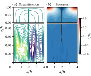
where $k\stackrel{\text{def}}{=}2\unicode[STIX]{x03C0}/\ell _{x}$. This choice is convenient for the analytic work in later sections. Figure 1 shows a two-dimensional solution ($\ell _{y}=0$) illustrating the formation of the buoyancy boundary layer adjacent to the non-uniform upper surface. The solution in figure 1 is unsteady due to vacillation of the plume.

Figure 1.

Panel (a) snapshot of stream function and (b) the buoyancy at $\unicode[STIX]{x1D705}t/h^{2}=0.6$. This is a no-stress solution with the sinusoidal $b_{s}$ in (2.4); control parameters are $Ra=6.4\times 10^{9}$, $Pr=1$, $\ell _{x}/h=4$ and $\ell _{y}=0$. This solution is unsteady and fluctuations in the attachment point of the plume to the upper surface $z=h$ break the midpoint symmetry of the circulation. The black contour in (b) is $b=-0.75b_{\star }$, which is close to the bottom buoyancy, defined as the $(x,t)$-average of $b$ at $z=0$.

The problem is characterized by four non-dimensional parameters: the Rayleigh and Prandtl numbers

(2.5a,b)$$\begin{eqnarray}Ra\,\stackrel{\text{def}}{=}\,\frac{\ell _{x}^{3}b_{\star }}{\unicode[STIX]{x1D708}\unicode[STIX]{x1D705}}\quad \text{and}\quad Pr\,\stackrel{\text{def}}{=}\,\frac{\unicode[STIX]{x1D708}}{\unicode[STIX]{x1D705}},\end{eqnarray}$$

and the aspect ratios $\ell _{x}/h$ and $\ell _{y}/h$.

In (2.4), the coordinate $x$ is distinguished by the assumption that the imposed surface buoyancy varies only along the $x$-axis. Hence the definition of $Ra$ in (2.5) employs $\ell _{x}$. Rosevear, Gayen & Griffiths (Reference Rosevear, Gayen and Griffiths2017) have recently considered surface buoyancy distributions with two-dimensional variation, such as $b_{s}\propto \sin ^{2}kx\sin ^{2}ky$. Here, however, we confine attention to the most basic version of HC in which variation of the surface buoyancy $b_{s}$ is only along the $x$-axis.

We use an overbar to denote an average over $x$, $y$ and $t$, taken at any fixed $z$ and $\langle \rangle$ to denote a total volume average over $x$, $y$, $z$ and $t$. Using this notation, we recall some results from Paparella & Young (Reference Paparella and Young2002) that are used below.

Horizontally averaging the buoyancy equation (2.2) we obtain the zero-flux constraint

(2.6)$$\begin{eqnarray}\overline{wb}-\unicode[STIX]{x1D705}\bar{b}_{z}=0.\end{eqnarray}$$

Taking , we obtain the kinetic energy power integral

(2.7)$$\begin{eqnarray}\unicode[STIX]{x1D700}=\langle wb\rangle ,\end{eqnarray}$$

where $\unicode[STIX]{x1D700}\stackrel{\text{def}}{=}\unicode[STIX]{x1D708}\langle |\unicode[STIX]{x1D735}\boldsymbol{u}|^{2}\rangle$ is the rate of dissipation of kinetic energy and $\langle wb\rangle$ is rate of conversion between potential and kinetic energy.

Vertically integrating (2.6) from $z=0$ to $h$, and setting the reference density $\unicode[STIX]{x1D70C}_{0}$ so that $\overline{b_{s}}=0$, we obtain another expression for $\langle wb\rangle$; substituting this into (2.7) we find

(2.8)$$\begin{eqnarray}\displaystyle h\unicode[STIX]{x1D700}=-\unicode[STIX]{x1D705}\bar{b}(0), & & \displaystyle\end{eqnarray}$$

(2.9)$$\begin{eqnarray}\displaystyle \leqslant \unicode[STIX]{x1D705}b_{\star }. & & \displaystyle\end{eqnarray}$$

In (2.8), $\bar{b}(0)$ is the $(x,y,t)$-average of the buoyancy at the bottom $z=0$. The inequality (2.9) follows from the extremum principle for the buoyancy advection-diffusion equation (2.2) with boundary condition (2.4).

In § 3 the inequality in (2.9) is employed to obtain $Ra\rightarrow \infty$ bounds on $Nu$. We have not been able to obtain an analytic estimate of the difference between $-\bar{b}(0)$ and the largest value allowed by the extremum principle, namely $b_{\star }$. However, in the example shown in figure 1, with $Ra=6.4\times 10^{9}$, the bottom buoyancy is $\bar{b}(0)\approx -0.755b_{\star }$ and thus the right of inequality (2.9) is approximately 33 % larger than $h\unicode[STIX]{x1D700}$. In figure 2 we show results from a suite of calculations with $Pr=1$ and varying $Ra$. These numerical results suggest, but do not prove, that as $Ra\rightarrow \infty$ the ratio $\bar{b}(0)/b_{\star }$ approaches a limiting value that is greater than $-1$. The solution in figure 1 is in this hypothetical regime: figure 2 shows that increasing $Ra$ by a factor of ten does not substantially change $\bar{b}(0)/b_{\star }$. Chiu-Webster, Hinch & Lister (Reference Chiu-Webster, Hinch and Lister2008) consider very viscous HC, that is $Pr=\infty$; their figure 25 shows $\bar{b}(0)/b_{\star }$ extrapolated to $Ra=\infty$. Based on this numerical result, Chiu-Webster et al. (Reference Chiu-Webster, Hinch and Lister2008) also conclude that the bottom buoyancy remains greater than the minimum value found on the upper surface. The main result from these numerical investigations is that inequality (2.9) entails an overestimate of $h\unicode[STIX]{x1D700}$ that in some cases is as large as 30 %.

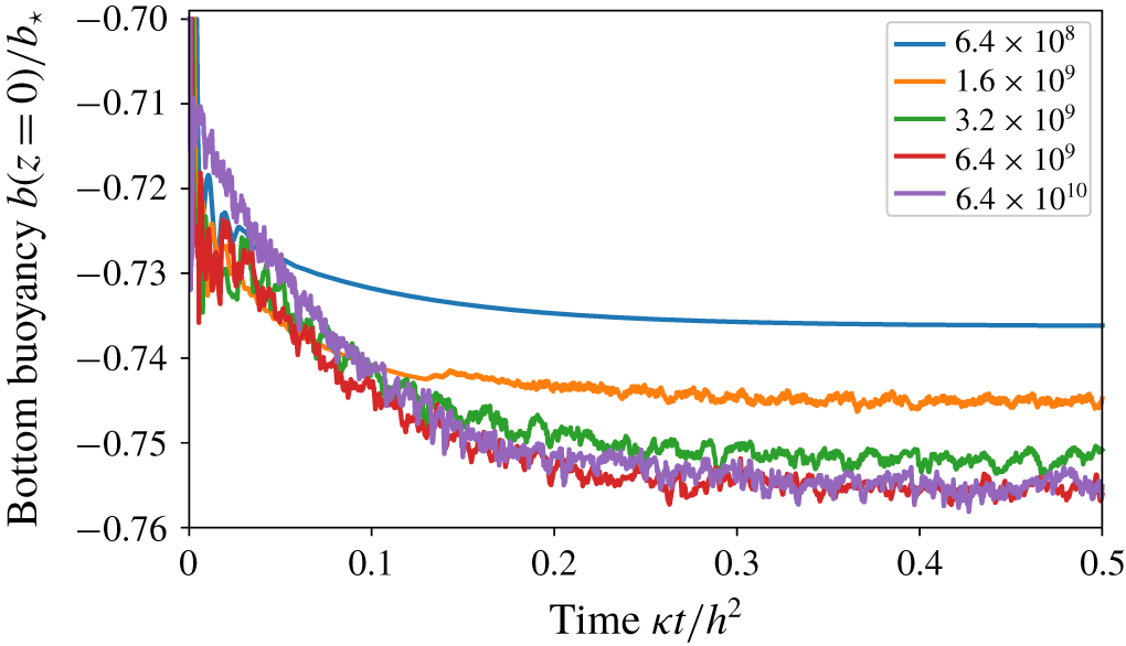
Figure 2.

The ‘instantaneous bottom buoyancy’, defined as an $(x,y)$-average of $b(x,y,0,t)$. This is a suite of five no-stress solutions with the sinusoidal $b_{s}$ in (2.4); all solutions started with initial buoyancy $-0.7b_{\star }$. Control parameters are $Pr=1$, $\ell _{x}/h=4$ and $\ell _{y}=0$ (two-dimensional solutions); the Rayleigh number $Ra$ is indicated in the legend. These computations were performed with tools developed by the Dedalus project: a spectral framework for solving partial differential equations (Burns et al. Reference Burns, Vasil, Oishi, Lecoanet and Brown2019, www.dedalus-project.org).

Young (Reference Young2010) shows that if the Mach number is zero, then the small divergence of the exact non-Boussinesq velocity, $\boldsymbol{U}$, due, for instance, to thermal expansion, can be diagnosed from within the Boussinesq approximation as $\unicode[STIX]{x1D735}\boldsymbol{\cdot }\boldsymbol{U}\approx \unicode[STIX]{x1D705}\unicode[STIX]{x0394}b/g$. Using this result, the energy source on the right of (2.8) can alternatively be written as $h\langle -z\unicode[STIX]{x1D705}\unicode[STIX]{x0394}b\rangle =\langle P\unicode[STIX]{x1D735}\boldsymbol{\cdot }\boldsymbol{U}\rangle$, where the total pressure $P$ is well approximated by the hydrostatic background $-\unicode[STIX]{x1D70C}_{0}gz$; see also the appendix of Wang & Huang (Reference Wang and Huang2005). In other words, the energy source on the right of (2.8) is the conversion of internal energy into kinetic energy by ‘piston work’ $-P\,\text{d}V$.

3 Bounds on the horizontal-convective Nusselt number

Siggers et al. (Reference Siggers, Kerswell and Balmforth2004) discuss the difficulty of defining the Nusselt number of HC. We follow Paparella & Young (Reference Paparella and Young2002) and SKB by first introducing the diffusive dissipation of buoyancy variance,

(3.1)$$\begin{eqnarray}\unicode[STIX]{x1D712}\,\stackrel{\text{def}}{=}\,\unicode[STIX]{x1D705}\langle |\unicode[STIX]{x1D735}b|^{2}\rangle .\end{eqnarray}$$

Then the Nusselt number is

(3.2)$$\begin{eqnarray}Nu\,\stackrel{\text{def}}{=}\,\frac{\unicode[STIX]{x1D712}}{\unicode[STIX]{x1D712}_{diff}},\end{eqnarray}$$

where $\unicode[STIX]{x1D712}_{diff}\stackrel{\text{def}}{=}\unicode[STIX]{x1D705}\langle |\unicode[STIX]{x1D735}b_{diff}|^{2}\rangle$ is the buoyancy dissipation of the diffusive solution i.e. $\unicode[STIX]{x1D705}\unicode[STIX]{x0394}b_{diff}=0$ with $b_{diff}$ satisfying the same boundary conditions as $b$.

An advantage in bounding $\unicode[STIX]{x1D712}$ for HC is that the elementary bound (2.9) takes care of the kinetic energy dissipation $\unicode[STIX]{x1D700}$. Bounds on HC are simpler than those of Rayleigh–Bénard convection because in the Rayleigh–Bénard problem it is necessary to deal with $\unicode[STIX]{x1D700}$ and $\unicode[STIX]{x1D712}$ simultaneously (Doering & Constantin Reference Doering and Constantin1996; Kerswell Reference Kerswell2001). In the HC problem the strategy is to first ignore the momentum equations (2.1) and obtain a bound on $\unicode[STIX]{x1D712}$ considering only the buoyancy equation (2.2) and incompressibility (2.3). The resulting bound in (3.17) below applies equally to a passive scalar and contains $\langle |\unicode[STIX]{x1D735}\boldsymbol{u}|^{2}\rangle$ (but not $\unicode[STIX]{x1D708}$). Dynamical information is then finally injected by replacing $\langle |\unicode[STIX]{x1D735}\boldsymbol{u}|^{2}\rangle$ with $\unicode[STIX]{x1D700}/\unicode[STIX]{x1D708}$ and using (2.9) to bound $\unicode[STIX]{x1D700}$. This approach identifies the $\unicode[STIX]{x1D700}$-bound in (2.9) as the only dynamical information incorporated into the $\unicode[STIX]{x1D712}$-bound.

We begin by introducing a ‘comparison function’, $c(\boldsymbol{x})$, which is any time-independent function that satisfies the same boundary conditions as $b(\boldsymbol{x},t)$: $c_{z}(x,y,0)=0$ and $c(x,y,h)=b_{s}(x)$. Forming , we find

(3.3)$$\begin{eqnarray}\unicode[STIX]{x1D712}=\unicode[STIX]{x1D705}\langle \unicode[STIX]{x1D735}b\boldsymbol{\cdot }\unicode[STIX]{x1D735}c\rangle -\langle b\boldsymbol{u}\boldsymbol{\cdot }\unicode[STIX]{x1D735}c\rangle .\end{eqnarray}$$

We use the comparison function

(3.4a,b)$$\begin{eqnarray}c=b_{s}(x)\,C(z)\quad \text{and}\quad C(z)\,\stackrel{\text{def}}{=}\,\frac{\cosh \unicode[STIX]{x1D707}z}{\cosh \unicode[STIX]{x1D707}h};\end{eqnarray}$$

(Balmforth & Young Reference Balmforth and Young2003; Winters & Young Reference Winters and Young2009). The parameter $\unicode[STIX]{x1D707}$ in (3.4) is later determined to optimize the $\unicode[STIX]{x1D712}$-bound. We consider a general surface buoyancy $b_{s}(x)$ and specialize to $b_{s}=b_{\star }\cos kx$ for numerical examples. With a general surface buoyancy profile we define the buoyancy scale as

(3.5)$$\begin{eqnarray}b_{\star }\,\stackrel{\text{def}}{=}\,\max _{x}|b_{s}(x)|,\end{eqnarray}$$

and represent the surface buoyancy as

(3.6)$$\begin{eqnarray}b_{s}(x)=b_{\star }\unicode[STIX]{x1D70F}(x),\end{eqnarray}$$

where the function $\unicode[STIX]{x1D70F}$ is dimensionless. Without loss of generality we choose the Boussinesq reference density $\unicode[STIX]{x1D70C}_{0}$ so that the horizontal average of $\unicode[STIX]{x1D70F}$ is zero: $\bar{\unicode[STIX]{x1D70F}}=0$.

As $\unicode[STIX]{x1D707}h\rightarrow \infty$ the comparison function (3.4) forms a boundary layer adjacent to the non-uniform surface at $z=h$. Thus the integrands on the right-hand side of the identity (3.3) are localized in the boundary layer at $z=h$. This observation shows that $\unicode[STIX]{x1D712}$ and $Nu$ can be determined solely by the statistical properties of $b$ and $\boldsymbol{u}$ within the boundary layer. Thus, at least as far as $Nu$ is concerned, conditions in the bulk of the flow can be ignored.

We decompose the buoyancy as

(3.7)$$\begin{eqnarray}b(\boldsymbol{x},t)=c(\boldsymbol{x})+a(\boldsymbol{x},t),\end{eqnarray}$$

so that $a(\boldsymbol{x},t)$ has homogeneous boundary conditions: $a(x,y,h,t)=0$ and $a_{z}(x,y,0,t)=0$. Substituting the decomposition (3.7) into (3.3) we find

(3.8)$$\begin{eqnarray}\unicode[STIX]{x1D712}=\unicode[STIX]{x1D705}\langle |\unicode[STIX]{x1D735}c|^{2}\rangle +\unicode[STIX]{x1D705}\langle \unicode[STIX]{x1D735}a\boldsymbol{\cdot }\unicode[STIX]{x1D735}c\rangle -\langle a\boldsymbol{u}\boldsymbol{\cdot }\unicode[STIX]{x1D735}c\rangle .\end{eqnarray}$$

An upper bound on $\unicode[STIX]{x1D712}$ follows from (3.8) by noting that there is an $\unicode[STIX]{x1D702}$ such that

(3.9)$$\begin{eqnarray}\big|\langle a\boldsymbol{u}\boldsymbol{\cdot }\unicode[STIX]{x1D735}c\rangle \big|\leqslant \unicode[STIX]{x1D702}\sqrt{\left\langle |\unicode[STIX]{x1D735}a|^{2}\right\rangle \left\langle |\unicode[STIX]{x1D735}\boldsymbol{u}|^{2}\right\rangle }.\end{eqnarray}$$

With the family of comparison functions in (3.4), $\unicode[STIX]{x1D702}$ is a function of $\unicode[STIX]{x1D707}$ that is most precisely determined by solving the variational problem sequestered in § 4. Following SKB and using Young’s inequality, equation (3.9) implies that

(3.10)$$\begin{eqnarray}\big|\langle a\boldsymbol{u}\boldsymbol{\cdot }\unicode[STIX]{x1D735}c\rangle \big|\leqslant {\textstyle \frac{1}{2}}\unicode[STIX]{x1D702}\left[\unicode[STIX]{x1D714}^{-1}\left\langle |\unicode[STIX]{x1D735}a|^{2}\right\rangle +\unicode[STIX]{x1D714}\left\langle |\unicode[STIX]{x1D735}\boldsymbol{u}|^{2}\right\rangle \right],\end{eqnarray}$$

where $\unicode[STIX]{x1D714}$ is any positive number. Substituting inequality (3.10) into the identity (3.8) one obtains

(3.11)$$\begin{eqnarray}\displaystyle \displaystyle \unicode[STIX]{x1D712} & {\leqslant} & \displaystyle \unicode[STIX]{x1D705}\langle |\unicode[STIX]{x1D735}c|^{2}\rangle +\unicode[STIX]{x1D705}\langle \unicode[STIX]{x1D735}a\boldsymbol{\cdot }\unicode[STIX]{x1D735}c\rangle +\frac{1}{2}\unicode[STIX]{x1D702}\unicode[STIX]{x1D714}^{-1}\left\langle |\unicode[STIX]{x1D735}a|^{2}\right\rangle +\frac{1}{2}\unicode[STIX]{x1D702}\unicode[STIX]{x1D714}\left\langle |\unicode[STIX]{x1D735}\boldsymbol{u}|^{2}\right\rangle ,\end{eqnarray}$$

(3.12)$$\begin{eqnarray}\displaystyle \displaystyle & = & \displaystyle \left(\unicode[STIX]{x1D705}-\frac{1}{2}\frac{\unicode[STIX]{x1D714}\unicode[STIX]{x1D705}^{2}}{\unicode[STIX]{x1D702}}\right)\langle |\unicode[STIX]{x1D735}c|^{2}\rangle +\frac{1}{2}\frac{\unicode[STIX]{x1D702}}{\unicode[STIX]{x1D714}}\left\langle |\unicode[STIX]{x1D735}a+\frac{\unicode[STIX]{x1D705}\unicode[STIX]{x1D714}}{\unicode[STIX]{x1D702}}\unicode[STIX]{x1D735}c|^{2}\right\rangle +\frac{1}{2}\unicode[STIX]{x1D702}\unicode[STIX]{x1D714}\left\langle |\unicode[STIX]{x1D735}\boldsymbol{u}|^{2}\right\rangle .\end{eqnarray}$$

Judiciously choosing $\unicode[STIX]{x1D714}=\unicode[STIX]{x1D702}/\unicode[STIX]{x1D705}$ makes the middle term on the right of (3.12) equal to $\unicode[STIX]{x1D712}/2$, so that (3.12) collapses to

(3.13)$$\begin{eqnarray}\unicode[STIX]{x1D712}\leqslant \unicode[STIX]{x1D705}\left\langle |\unicode[STIX]{x1D735}c|^{2}\right\rangle +\frac{\unicode[STIX]{x1D702}^{2}}{\unicode[STIX]{x1D705}}\left\langle |\unicode[STIX]{x1D735}\boldsymbol{u}|^{2}\right\rangle .\end{eqnarray}$$

The inequality (3.13) is the main tool used to upper-bound $Nu$ in (3.2).

The next step is to determine the dependence of $\unicode[STIX]{x1D702}$ on the boundary-layer parameter $\unicode[STIX]{x1D707}$ in the limit $\unicode[STIX]{x1D707}\rightarrow \infty$. The result from § 4 is that as $\unicode[STIX]{x1D707}\rightarrow \infty$

(3.14)$$\begin{eqnarray}\unicode[STIX]{x1D702}\sim K\frac{b_{\star }}{\unicode[STIX]{x1D707}},\end{eqnarray}$$

where the non-dimensional factor $K$ depends on the surface-buoyancy shape function $\unicode[STIX]{x1D70F}(x)$, the viscous boundary condition, but not the aspect ratio of the domain e.g. for $\unicode[STIX]{x1D70F}=\cos kx$ see (4.51) and (4.52). We proceed by substituting the $\unicode[STIX]{x1D707}\rightarrow \infty$ asymptotic result (3.14) into (3.13). Evaluating the first term on the right of (3.13) in the $\unicode[STIX]{x1D707}\rightarrow \infty$ limit we then have an asymptotic inequality

(3.15)$$\begin{eqnarray}\unicode[STIX]{x1D712}\lesssim \frac{\unicode[STIX]{x1D705}b_{\star }^{2}\overline{\unicode[STIX]{x1D70F}^{2}}}{2h}\unicode[STIX]{x1D707}+\frac{K^{2}b_{\star }^{2}\langle |\unicode[STIX]{x1D735}\boldsymbol{u}|^{2}\rangle }{\unicode[STIX]{x1D705}\unicode[STIX]{x1D707}^{2}}.\end{eqnarray}$$

The best upper bound on $\unicode[STIX]{x1D712}$ is obtained by finding the $\unicode[STIX]{x1D707}$ that minimizes the right-hand side of (3.15). This is

(3.16)$$\begin{eqnarray}\unicode[STIX]{x1D707}=\left(\frac{4K^{2}\langle |\unicode[STIX]{x1D735}\boldsymbol{u}|^{2}\rangle h}{\overline{\unicode[STIX]{x1D70F}^{2}}\unicode[STIX]{x1D705}^{2}}\right)^{1/3}.\end{eqnarray}$$

The best upper bound is therefore

(3.17)$$\begin{eqnarray}\unicode[STIX]{x1D712}\lesssim 3\left(\frac{K\overline{\unicode[STIX]{x1D70F}^{2}}}{4}\right)^{2/3}\left(\frac{\unicode[STIX]{x1D705}\langle |\unicode[STIX]{x1D735}\boldsymbol{u}|^{2}\rangle }{h^{2}}\right)^{1/3}b_{\star }^{2}.\end{eqnarray}$$

The bound in (3.17) follows from the buoyancy equation (2.2) and the incompressibility condition (2.3) – the momentum equation has not been used. Dynamical information is supplied using inequality (2.9) to bound $\langle |\unicode[STIX]{x1D735}\boldsymbol{u}|^{2}\rangle$ in (3.17) by $\unicode[STIX]{x1D705}b_{\star }/\unicode[STIX]{x1D708}h$, resulting in

(3.18)$$\begin{eqnarray}\unicode[STIX]{x1D712}\lesssim \underbrace{3\left(\frac{K\overline{\unicode[STIX]{x1D70F}^{2}}}{4}\right)^{2/3}}_{\stackrel{\text{def}}{=}C_{\unicode[STIX]{x1D712}}}\left(\frac{\unicode[STIX]{x1D705}^{2}}{\unicode[STIX]{x1D708}h^{3}}\right)^{1/3}b_{\star }^{7/3}.\end{eqnarray}$$

After normalization by $\unicode[STIX]{x1D712}_{diff}$, (3.18) results in the $Ra^{1/3}$-bound in (1.1).

Using $b_{s}(x)=b_{\star }\cos kx$ as an illustration, we express (3.18) in non-dimensional variables. In this case $\overline{\unicode[STIX]{x1D70F}^{2}}=1/2$ and $\unicode[STIX]{x1D712}_{diff}=\unicode[STIX]{x1D705}kb_{\star }^{2}\tanh kh/(2h)$, so that

(3.19)$$\begin{eqnarray}Nu\lesssim \underbrace{\frac{3K^{2/3}}{4\unicode[STIX]{x03C0}}}_{\stackrel{\text{def}}{=}C_{Nu}}\coth khRa^{1/3}.\end{eqnarray}$$

The aspect ratio, $h/\ell _{x}=kh/(2\unicode[STIX]{x03C0})$, enters the bound only through the normalization factor $\unicode[STIX]{x1D712}_{diff}$: the constant $C_{\unicode[STIX]{x1D712}}$ in (3.18) does not depend on aspect ratio.

We have four different estimates of the constant $K$, leading to four different values for the prefactor $C_{Nu}$ in (3.19). The simplest results for $C_{Nu}$ follow from the asymptotic inequalities of SKB,

(3.20)$$\begin{eqnarray}C_{Nu}^{SKB}=\frac{3}{2^{2/3}\unicode[STIX]{x03C0}^{7/3}}=0.1307.\end{eqnarray}$$

The analogous result from appendix A is $K=0.3458$ in (A 14), so that

(3.21)$$\begin{eqnarray}C_{Nu}^{\,Appendix}=0.1176.\end{eqnarray}$$

The values of $C_{Nu}$ above are independent of boundary conditions. More precise results for $K$ are provided by the solution of the variational problem in § 4, culminating in the exact asymptotic expressions for $K$ in (4.51) and (4.52). These result in

(3.22a,b)$$\begin{eqnarray}C_{Nu}^{\,no\,slip}=0.0525\quad \text{and}\quad C_{Nu}^{\,no\,stress}=0.0808.\end{eqnarray}$$

It is remarkable that the relatively crude estimates in (3.20) and (3.21) are so close to (3.22).

The bounds in (3.22) are based on the $\cosh \unicode[STIX]{x1D707}z$ comparison function introduced in (3.6). Further improvements might be possible with other comparison functions, or perhaps by strengthening the bound on kinetic energy dissipation in (2.9) so that it agrees more closely with clues provided by the numerical solution of figure 2. The results from § 4, however, show that such improvements will not alter the exponent $1/3$ in (3.19): the $1/3$ is a consequence of $\unicode[STIX]{x1D702}\sim \unicode[STIX]{x1D707}^{-1}$ in (3.14), and we now proceed to show constructively that there are trial functions that achieve $\unicode[STIX]{x1D702}\sim \unicode[STIX]{x1D707}^{-1}$.

4 The variational problem for $\unicode[STIX]{x1D702}$

The quantity $\unicode[STIX]{x1D702}$, introduced in (3.9), is defined as

(4.1)$$\begin{eqnarray}\unicode[STIX]{x1D702}\,\stackrel{\text{def}}{=}\,\max _{\unicode[STIX]{x1D703},\boldsymbol{v}}\frac{|\langle \unicode[STIX]{x1D703}\boldsymbol{v}\boldsymbol{\cdot }\unicode[STIX]{x1D735}c\rangle |}{\sqrt{\langle |\unicode[STIX]{x1D735}\unicode[STIX]{x1D703}|^{2}\rangle \langle |\unicode[STIX]{x1D735}\boldsymbol{v}|^{2}\rangle }},\end{eqnarray}$$

where the incompressible vector field $\boldsymbol{v}$ satisfies the same homogeneous boundary conditions as $\boldsymbol{u}$ and the scalar field $\unicode[STIX]{x1D703}$ satisfies the same homogeneous boundary conditions as $a$ in (3.7). The comparison function $c(x,z;\unicode[STIX]{x1D707})$ is defined in (3.4) and we are interested in the boundary-layer limit $\unicode[STIX]{x1D707}\rightarrow \infty$ corresponding to $Ra\rightarrow \infty$.

The SKB-type inequalities in appendix A result in

(4.2)$$\begin{eqnarray}\unicode[STIX]{x1D702}\lesssim 0.3458\frac{b_{\star }}{\unicode[STIX]{x1D707}},\quad \text{as }\unicode[STIX]{x1D707}\rightarrow \infty .\end{eqnarray}$$

Appendix A, however, does not exhibit $(\boldsymbol{v},\unicode[STIX]{x1D703})$ that actually achieve the $\unicode[STIX]{x1D702}\sim \unicode[STIX]{x1D707}^{-1}$ scaling suggested by the asymptotic inequality in (4.2), and nor do SKB. Thus it is possible that $\unicode[STIX]{x1D702}\lesssim \unicode[STIX]{x1D707}^{-n}$ with an exponent $n$ that is larger than $1$: this would be consistent with inequality (4.2). One might expect that it would be easy to settle this question by guessing a ‘trial’ $(\boldsymbol{v},\unicode[STIX]{x1D703})$ that achieves the scaling $\unicode[STIX]{x1D702}\sim \unicode[STIX]{x1D707}^{-1}$ suggested by (4.2). We found, however, that ‘obvious’ guesses at $(\unicode[STIX]{x1D703},\boldsymbol{v})$ resulted in $\unicode[STIX]{x1D707}^{-2}$ for no-slip boundary conditions and $\unicode[STIX]{x1D707}^{-3/2}$ for no-stress. Via (3.17), these alternative asymptotic inequalities would dramatically lower the $1/3$ exponent in (1.1) to $1/5$ and $1/4$, respectively. Unfortunately the obvious guesses do not at all resemble the optimal $(\boldsymbol{v},\unicode[STIX]{x1D703})$ determined in this section.

(Another way to view the inequalities in appendix A is to say that the optimal solution determined there is exhibited as a velocity field with $u=v=0$ and with $b(z)$ and $w(z)$ as the functions $\unicode[STIX]{x1D703}(z)$ and $\unicode[STIX]{x1D714}(z)$ that optimize the functionals in (A 6). The ‘one-dimensional’ velocity field $\boldsymbol{u}=\unicode[STIX]{x1D714}(z)\hat{\boldsymbol{z}}$ does not satisfy the continuity equation (2.3). In this sense, the inequalities in appendix A do not take full advantage of $\unicode[STIX]{x1D735}\boldsymbol{\cdot }\boldsymbol{u}=0$.)

The main result of this section is to establish the asymptotic equality in (3.14) by showing that there are $(\boldsymbol{v},\unicode[STIX]{x1D703})$, with $\unicode[STIX]{x1D735}\boldsymbol{\cdot }\boldsymbol{v}=0$, that actually produce the $\unicode[STIX]{x1D707}^{-1}$ scaling suggested by (4.2). We also calculate the constant $K$ in (3.14); unlike the constant $0.3485$ in (4.2), this $K$ depends on the choice between no-stress and no-slip boundary conditions and provides the strongest version of the upper bound on $\unicode[STIX]{x1D712}$ in (3.13).

4.1 A variational problem

The straightforward approach to obtaining $\unicode[STIX]{x1D702}$ in (4.1) is to calculate the maximum of the right-hand side using variational methods. With this hope, one can reformulate the problem posed in (4.1) by introducing the constrained functional

(4.3)$$\begin{eqnarray}{\mathcal{E}}[\boldsymbol{v},\unicode[STIX]{x1D703}]\,\stackrel{\text{def}}{=}\,\langle \unicode[STIX]{x1D703}\boldsymbol{v}\boldsymbol{\cdot }\unicode[STIX]{x1D735}c\rangle -\langle \unicode[STIX]{x1D719}\unicode[STIX]{x1D735}\boldsymbol{\cdot }\boldsymbol{v}\rangle +{\textstyle \frac{1}{2}}\unicode[STIX]{x1D709}[\langle |\unicode[STIX]{x1D735}\boldsymbol{v}|^{2}\rangle -1]+{\textstyle \frac{1}{2}}\unicode[STIX]{x1D702}[\langle |\unicode[STIX]{x1D735}\unicode[STIX]{x1D703}|^{2}\rangle -1].\end{eqnarray}$$

In (4.3) the Lagrange multipliers $\unicode[STIX]{x1D709}$ and $\unicode[STIX]{x1D702}$ ensure normalization of $\unicode[STIX]{x1D703}$ and $\boldsymbol{v}$, and $\unicode[STIX]{x1D719}(\boldsymbol{x})$ enforces incompressibility of $\boldsymbol{v}$.

The Euler–Lagrange equations corresponding to extremization of (4.3) are

(4.4)$$\begin{eqnarray}\displaystyle & \displaystyle \frac{\unicode[STIX]{x1D6FF}{\mathcal{E}}}{\unicode[STIX]{x1D6FF}\unicode[STIX]{x1D703}}=0:\quad \boldsymbol{v}\boldsymbol{\cdot }\unicode[STIX]{x1D735}c=\unicode[STIX]{x1D702}\unicode[STIX]{x0394}\unicode[STIX]{x1D703}, & \displaystyle\end{eqnarray}$$

(4.5)$$\begin{eqnarray}\displaystyle & \displaystyle \frac{\unicode[STIX]{x1D6FF}{\mathcal{E}}}{\unicode[STIX]{x1D6FF}\boldsymbol{v}}=0:\quad \unicode[STIX]{x1D703}\unicode[STIX]{x1D735}c+\unicode[STIX]{x1D735}\unicode[STIX]{x1D719}=\unicode[STIX]{x1D709}\unicode[STIX]{x0394}\boldsymbol{v}, & \displaystyle\end{eqnarray}$$

(4.6)$$\begin{eqnarray}\displaystyle & \displaystyle \frac{\unicode[STIX]{x1D6FF}{\mathcal{E}}}{\unicode[STIX]{x1D6FF}\unicode[STIX]{x1D719}}=0:\quad \unicode[STIX]{x1D735}\boldsymbol{\cdot }\boldsymbol{v}=0. & \displaystyle\end{eqnarray}$$

Note that if $(\unicode[STIX]{x1D703},\boldsymbol{v},\unicode[STIX]{x1D719},\unicode[STIX]{x1D709},\unicode[STIX]{x1D702})$ is a solution of the Euler–Lagrange equations above then so is $(-\unicode[STIX]{x1D703},\boldsymbol{v},-\unicode[STIX]{x1D719},-\unicode[STIX]{x1D709},-\unicode[STIX]{x1D702})$. This transformation flips the sign of $\langle \unicode[STIX]{x1D703}\boldsymbol{v}\boldsymbol{\cdot }\unicode[STIX]{x1D735}c\rangle$. Thus if $(\unicode[STIX]{x1D703},\boldsymbol{v},\unicode[STIX]{x1D719},\unicode[STIX]{x1D709},\unicode[STIX]{x1D702})$ is a minimum of ${\mathcal{E}}$ then $(-\unicode[STIX]{x1D703},\boldsymbol{v},-\unicode[STIX]{x1D719},-\unicode[STIX]{x1D709},-\unicode[STIX]{x1D702})$ is a maximum.

Forming and one has

(4.7a,b)$$\begin{eqnarray}-\left\langle \unicode[STIX]{x1D703}\boldsymbol{v}\boldsymbol{\cdot }\unicode[STIX]{x1D735}c\right\rangle =\unicode[STIX]{x1D702}\underbrace{\left\langle |\unicode[STIX]{x1D735}\unicode[STIX]{x1D703}|^{2}\right\rangle }_{=1}\quad \text{and}\quad -\left\langle \unicode[STIX]{x1D703}\boldsymbol{v}\boldsymbol{\cdot }\unicode[STIX]{x1D735}c\right\rangle =\unicode[STIX]{x1D709}\underbrace{\left\langle |\unicode[STIX]{x1D735}\boldsymbol{v}|^{2}\right\rangle }_{=1}.\end{eqnarray}$$

The identities (4.7) imply that

(4.8)$$\begin{eqnarray}\unicode[STIX]{x1D709}=\unicode[STIX]{x1D702},\end{eqnarray}$$

and so we can regard the system in (4.4) through to (4.6) as an eigenproblem with eigenvalue $\unicode[STIX]{x1D702}$. We take $\unicode[STIX]{x1D709}=\unicode[STIX]{x1D702}>0$ and it follows from (4.7) that we are seeking the most negative value of $\left\langle \unicode[STIX]{x1D703}\boldsymbol{v}\boldsymbol{\cdot }\unicode[STIX]{x1D735}c\right\rangle$, corresponding to the largest positive value of $\unicode[STIX]{x1D702}$. In other words, $\unicode[STIX]{x1D702}$ in (4.1) is the most positive eigenvalue of the Euler–Lagrange equations (4.4) through to (4.6), and from the identities in (4.7)

(4.9)$$\begin{eqnarray}\unicode[STIX]{x1D702}=-\min _{\forall \boldsymbol{v},\unicode[STIX]{x1D703}}{\mathcal{E}}[\boldsymbol{v},\unicode[STIX]{x1D703}]=\max _{\forall \,\boldsymbol{v},\unicode[STIX]{x1D703}}{\mathcal{E}}[\boldsymbol{v},\unicode[STIX]{x1D703}].\end{eqnarray}$$

Thus the Lagrange multiplier $\unicode[STIX]{x1D702}$ in (4.3) is the same as the $\unicode[STIX]{x1D702}$ in (3.9) and (4.1).

We begin by considering two-dimensional solutions with a stream function $\unicode[STIX]{x1D713}$ such as

(4.10)$$\begin{eqnarray}\boldsymbol{v}=(\unicode[STIX]{x1D713}_{z},0,-\unicode[STIX]{x1D713}_{x}).\end{eqnarray}$$

With this simplification, the Euler–Lagrange equations in (4.4) through to (4.6) reduce to

(4.11)$$\begin{eqnarray}\displaystyle & \displaystyle c_{x}\unicode[STIX]{x1D713}_{z}-c_{z}\unicode[STIX]{x1D713}_{x}=\unicode[STIX]{x1D702}\unicode[STIX]{x0394}\unicode[STIX]{x1D703}, & \displaystyle\end{eqnarray}$$

(4.12)$$\begin{eqnarray}\displaystyle & \displaystyle c_{x}\unicode[STIX]{x1D703}_{z}-c_{z}\unicode[STIX]{x1D703}_{x}=\unicode[STIX]{x1D702}\unicode[STIX]{x1D6E5}^{2}\unicode[STIX]{x1D713}. & \displaystyle\end{eqnarray}$$

In terms of $\unicode[STIX]{x1D713}$ and $\unicode[STIX]{x1D703}$, the functional in (4.3) is

(4.13)$$\begin{eqnarray}{\mathcal{E}}[\unicode[STIX]{x1D713},\unicode[STIX]{x1D703}]=\langle \unicode[STIX]{x1D703}J(c,\unicode[STIX]{x1D713})\rangle +{\textstyle \frac{1}{2}}\unicode[STIX]{x1D702}\left[\left\langle (\unicode[STIX]{x0394}\unicode[STIX]{x1D713})^{2}\right\rangle -1\right]+{\textstyle \frac{1}{2}}\unicode[STIX]{x1D702}\left[\left\langle |\unicode[STIX]{x1D735}\unicode[STIX]{x1D703}|^{2}\right\rangle -1\right].\end{eqnarray}$$

We attempted a numerical assault on (4.11) and (4.12). This failed miserably: we show below in § 4.5 that as $\unicode[STIX]{x1D707}\rightarrow \infty$ the numerical solution develops small-scale oscillations in $x$ with a wavelength ${\sim}\unicode[STIX]{x1D707}^{-1}$. The solution is also boundary layered in $z$. Given the boundary-layer structure of the comparison function $c(x,z;\unicode[STIX]{x1D707})$ in (3.3), the boundary layer in $(\unicode[STIX]{x1D713},\unicode[STIX]{x1D703})$ was expected and was built into our numerical solution. The fast oscillation in $x$, however, was not anticipated. Consequently the available $x$-resolution became inadequate at only moderately large values of $\unicode[STIX]{x1D707}$ and it was not possible to make a reliable estimate of $\unicode[STIX]{x1D702}$ in the limit $\unicode[STIX]{x1D707}\rightarrow \infty$. But once one is alerted to the existence of rapid oscillations, the Wentzel–Kramers–Brillouin (WKB) method is suggested as a means of attacking (4.11) and (4.12). Moreover, with this insight, it is also easy to manufacture trial functions that produce the asymptotic lower bounds of the form

(4.14)$$\begin{eqnarray}K^{low}\frac{b_{\star }}{\unicode[STIX]{x1D707}}<\unicode[STIX]{x1D702}.\end{eqnarray}$$

These trial-function lower bounds are complementary to the upper bound in (4.2) and show definitively that $\unicode[STIX]{x1D702}$ is proportional to $\unicode[STIX]{x1D707}^{-1}$ as $\unicode[STIX]{x1D707}\rightarrow \infty$. Moreover, one can systematically judge the quality of trial functions: the best trial function produces the largest value of $K^{low}$. We found that systematic examination of three trial functions developed the intuition that is required to successfully apply the WKB method to (4.11) and (4.12). Thus we begin by estimating $K^{low}$ with trial functions.

(As for the miserable failure mentioned above: we applied a Fourier series in $x$ to (4.11) and (4.12). With the sinusoidal $b_{s}$ in (2.4), symmetry considerations show that the series has the form

(4.15)$$\begin{eqnarray}\displaystyle & \displaystyle \unicode[STIX]{x1D713}=\hat{\unicode[STIX]{x1D713}}_{1}(z)\sin kx+\hat{\unicode[STIX]{x1D713}}_{3}(z)\sin 3kx+\cdots & \displaystyle\end{eqnarray}$$

(4.16)$$\begin{eqnarray}\displaystyle & \displaystyle \unicode[STIX]{x1D703}=\hat{\unicode[STIX]{x1D703}}_{0}(z)+\hat{\unicode[STIX]{x1D703}}_{2}(z)\cos 2kx+\hat{\unicode[STIX]{x1D703}}_{4}(z)\cos 4kx+\cdots & \displaystyle\end{eqnarray}$$

The most efficient approach is to keep $N$ terms in the $\unicode[STIX]{x1D713}$-series and $N+1$ in the $\unicode[STIX]{x1D703}$-series. The Galerkin method was used to obtain a system of $2N+1$ ordinary differential equations in $z$, with analytically determined coefficients. We then solved the resulting eigenvalue problem for $\unicode[STIX]{x1D702}$ using Matlab’s bvp5c boundary value solver (a collocation method). For given $\unicode[STIX]{x1D707}$, increasing $N$ eventually results in satisfactory convergence of the eigenvalue $\unicode[STIX]{x1D702}$. For example, with $\unicode[STIX]{x1D707}=10$, $N=5$ was enough. But as $\unicode[STIX]{x1D707}$ is increased, ever larger values of $N$ are required for convergence, indicating that the solution is developing ever smaller scales in $x$. With hindsight, we see that (4.15) and (4.16) are attempting to represent a large-$\unicode[STIX]{x1D707}$ solution such as the example shown figure 3; this requires $N$ of order 1000. As $\unicode[STIX]{x1D707}\rightarrow \infty$, $\unicode[STIX]{x1D702}\sim \unicode[STIX]{x1D707}^{-\unicode[STIX]{x1D712}}$ and a main goal is to determine the exponent $\unicode[STIX]{x1D712}$. But the values of $\unicode[STIX]{x1D707}$ that were accessible with truncations of (4.15) and (4.16) were too small to reliably indicate the exponent $\unicode[STIX]{x1D712}$. The result $\unicode[STIX]{x1D712}=1$ follows from numerically assisted application of the WKB approximation in § 4.5.)

4.2 The first trial function

The first trial function we consider is

(4.17a,b)$$\begin{eqnarray}\unicode[STIX]{x1D713}_{1}=a_{\unicode[STIX]{x1D713}}\,\text{e}^{\unicode[STIX]{x1D6FC}Z}Z^{2}\sin \unicode[STIX]{x1D707}S\quad \text{and}\quad \unicode[STIX]{x1D703}_{1}=a_{\unicode[STIX]{x1D703}}\,\text{e}^{\unicode[STIX]{x1D6FC}Z}Z\cos \unicode[STIX]{x1D707}S,\end{eqnarray}$$

where $Z\stackrel{\text{def}}{=}\unicode[STIX]{x1D707}(z-h)$ and

(4.18)$$\begin{eqnarray}S(x)\,\stackrel{\text{def}}{=}\,\unicode[STIX]{x1D6FE}\int _{0}^{x}\unicode[STIX]{x1D70F}(x^{\prime })\,\text{d}x^{\prime }.\end{eqnarray}$$

In (4.18), $\unicode[STIX]{x1D70F}$ is the dimensionless surface buoyancy introduced in (3.6) and the disposable constants $\unicode[STIX]{x1D6FC}$ and $\unicode[STIX]{x1D6FE}$ are selected to maximize ${\mathcal{E}}[\boldsymbol{v},\unicode[STIX]{x1D703}]$. The amplitudes $a_{\unicode[STIX]{x1D713}}$ and $a_{\unicode[STIX]{x1D703}}$ in (4.17) are determined by enforcing the normalization conditions that $\langle (\unicode[STIX]{x0394}\unicode[STIX]{x1D713})^{2}\rangle =\langle |\unicode[STIX]{x1D735}\unicode[STIX]{x1D703}|^{2}\rangle =1$. The trial function $\unicode[STIX]{x1D713}_{1}$ in (4.17) satisfies no-slip conditions at the top surface (corresponding to $Z=0$). In the limit $h\unicode[STIX]{x1D707}\rightarrow \infty$ one can safely ignore the bottom boundary conditions where both the comparison function $c(x,z;\unicode[STIX]{x1D707})$ and the trial functions are exponentially small.

The non-obvious aspect of the trial function in (4.17) is the rapid oscillation of $\cos \unicode[STIX]{x1D707}S$ and $\sin \unicode[STIX]{x1D707}S$ in the limit $\unicode[STIX]{x1D707}\rightarrow \infty$. This rapid oscillation of the variational solution is key to all results in this section.

Now we evaluate the functional ${\mathcal{E}}[\boldsymbol{v}_{1},\unicode[STIX]{x1D703}_{1}]$ using (4.17). We freely use $\unicode[STIX]{x1D707}\rightarrow \infty$ to evaluate all $x$-integrals; typical $\unicode[STIX]{x1D707}\rightarrow \infty$ simplifications are

(4.19a,b)$$\begin{eqnarray}\displaystyle \overline{\unicode[STIX]{x1D70F}(x)^{2}\,\sin ^{2}\unicode[STIX]{x1D707}S}\rightarrow {\textstyle \frac{1}{2}}\overline{\unicode[STIX]{x1D70F}^{2}},\quad \overline{\unicode[STIX]{x1D70F}(x)^{4}\,\sin ^{2}\unicode[STIX]{x1D707}S}\rightarrow {\textstyle \frac{1}{2}}\overline{\unicode[STIX]{x1D70F}^{4}}, & & \displaystyle\end{eqnarray}$$

(4.20a,b)$$\begin{eqnarray}\displaystyle \overline{\unicode[STIX]{x1D70F}_{x}(x)^{2}\cos ^{2}\unicode[STIX]{x1D707}S}\rightarrow {\textstyle \frac{1}{2}}\overline{\unicode[STIX]{x1D70F}_{x}^{2}},\quad \overline{\unicode[STIX]{x1D70F}^{\prime }(x)\,\unicode[STIX]{x1D70F}(x)^{2}\,\sin \unicode[STIX]{x1D707}S\,\cos \unicode[STIX]{x1D707}S}\rightarrow 0, & & \displaystyle\end{eqnarray}$$

where the overbar denotes an $x$-average. After some calculation we find that the normalization conditions are

(4.21)$$\begin{eqnarray}\displaystyle & \displaystyle 1=\frac{a_{\unicode[STIX]{x1D713}}^{2}\unicode[STIX]{x1D707}^{3}}{8\unicode[STIX]{x1D6FC}h}(3+2r^{2}\overline{\unicode[STIX]{x1D70F}^{2}}+3\overline{\unicode[STIX]{x1D70F}^{4}}r^{4})+\frac{3a_{\unicode[STIX]{x1D713}}^{2}\unicode[STIX]{x1D707}}{16\unicode[STIX]{x1D6FC}^{3}h}r^{2}\overline{\unicode[STIX]{x1D70F}_{x}^{2}}, & \displaystyle\end{eqnarray}$$

(4.22)$$\begin{eqnarray}\displaystyle & \displaystyle 1=\frac{a_{\unicode[STIX]{x1D703}}^{2}\unicode[STIX]{x1D707}}{8\unicode[STIX]{x1D6FC}h}(1+\overline{\unicode[STIX]{x1D70F}^{2}}r^{2}), & \displaystyle\end{eqnarray}$$

where $r\stackrel{\text{def}}{=}\unicode[STIX]{x1D6FE}/\unicode[STIX]{x1D6FC}$. We drop the final $O(\unicode[STIX]{x1D707})$ term in (4.21) relative to the much larger $\unicode[STIX]{x1D707}^{3}$ term.

After the normalization conditions are applied, the functional is

(4.23)$$\begin{eqnarray}{\mathcal{E}}[\boldsymbol{v}_{1},\unicode[STIX]{x1D703}_{1}]=\underbrace{\langle \unicode[STIX]{x1D703}_{1}\unicode[STIX]{x1D713}_{1z}c_{x}\rangle }_{{\sim}\unicode[STIX]{x1D707}^{-2}}-\underbrace{\langle \unicode[STIX]{x1D703}_{1}\unicode[STIX]{x1D713}_{1x}c_{z}\rangle }_{{\sim}\unicode[STIX]{x1D707}^{-1}}.\end{eqnarray}$$

Thus, as in the upper bound in (A 5), only the vertical advection by $\unicode[STIX]{x1D713}_{1x}$ is asymptotically important. The leading-order approximation to the functional is then

(4.24)$$\begin{eqnarray}\displaystyle {\mathcal{E}}[\boldsymbol{v}_{1},\unicode[STIX]{x1D703}_{1}] & = & \displaystyle \displaystyle \frac{3\overline{\unicode[STIX]{x1D70F}^{2}}b_{\star }\unicode[STIX]{x1D707}}{h}\frac{a_{\unicode[STIX]{x1D713}}a_{\unicode[STIX]{x1D703}}\unicode[STIX]{x1D6FE}}{(1+2\unicode[STIX]{x1D6FC})^{4}},\end{eqnarray}$$

(4.25)$$\begin{eqnarray}\displaystyle & = & \displaystyle \displaystyle \frac{96\overline{\unicode[STIX]{x1D70F}^{2}}b_{\star }}{\unicode[STIX]{x1D707}}\frac{r}{\sqrt{(24+16\overline{\unicode[STIX]{x1D70F}^{2}}\,r^{2}+24\overline{\unicode[STIX]{x1D70F}^{4}}\,r^{4})(2+2\overline{\unicode[STIX]{x1D70F}^{2}}\,r^{2})}}\frac{\unicode[STIX]{x1D6FC}^{2}}{(1+2\unicode[STIX]{x1D6FC})^{4}}.\end{eqnarray}$$

The parameters $\unicode[STIX]{x1D6FC}$ and $r=\unicode[STIX]{x1D6FE}/\unicode[STIX]{x1D6FC}$ are determined so as to maximize ${\mathcal{E}}[\boldsymbol{v}_{1},\unicode[STIX]{x1D703}_{1}]$. Thus $\unicode[STIX]{x1D6FC}=1/2$ for all $\unicode[STIX]{x1D70F}$. With $\unicode[STIX]{x1D70F}(x)=\cos kx$ we have $\overline{\unicode[STIX]{x1D70F}^{2}}=1/2$ and $\overline{\unicode[STIX]{x1D70F}^{4}}=3/8$. In this case, the optimal value of $r=\unicode[STIX]{x1D6FE}/\unicode[STIX]{x1D6FC}$ is $1.01819$ and

(4.26)$$\begin{eqnarray}{\mathcal{E}}[\boldsymbol{v}_{1},\unicode[STIX]{x1D703}_{1}]\sim \underbrace{0.0676451}_{\stackrel{\text{def}}{=}K_{1}^{low}}\,\frac{b_{\star }}{\unicode[STIX]{x1D707}}.\end{eqnarray}$$

The constant $K_{1}^{low}$ is smaller by a factor of approximately $5$ than the upper-bound constant $0.3458$ in (4.2).

4.3 The second trial function

To obtain a larger value of $K^{low}$ we consider a second trial function with the same horizontal structure as $(\unicode[STIX]{x1D713}_{1},\unicode[STIX]{x1D703}_{1})$, but with general $z$-structure

(4.27a,b)$$\begin{eqnarray}\unicode[STIX]{x1D713}_{2}=\unicode[STIX]{x1D707}^{-3/2}P(Z)\sin \unicode[STIX]{x1D707}S\quad \text{and}\quad \unicode[STIX]{x1D703}_{2}=\unicode[STIX]{x1D707}^{-1/2}T(Z)\cos \unicode[STIX]{x1D707}S.\end{eqnarray}$$

Here $S(x)$ is defined in (4.18). The factors $\unicode[STIX]{x1D707}^{-3/2}$ and $\unicode[STIX]{x1D707}^{-1/2}$ are included so that $P$ and $T$ are order unity as $\unicode[STIX]{x1D707}\rightarrow \infty$. Using simplifications such as (4.19) and (4.20) one can evaluate the $x$-integrals in the functional ${\mathcal{E}}[\boldsymbol{v}_{2},\unicode[STIX]{x1D703}_{2}]$ to obtain

(4.28)$$\begin{eqnarray}\displaystyle {\mathcal{E}}[\boldsymbol{v}_{2},\unicode[STIX]{x1D703}_{2}] & = & \displaystyle \displaystyle -\frac{b_{\star }\overline{\unicode[STIX]{x1D70F}^{2}}\,\unicode[STIX]{x1D6FE}}{2h\unicode[STIX]{x1D707}}\int _{-\infty }^{0}\text{e}^{Z}TP\,\text{d}Z+\frac{1}{2}\unicode[STIX]{x1D702}\left[\frac{1}{2h}\int _{-\infty }^{0}T_{Z}^{2}+\overline{\unicode[STIX]{x1D70F}^{2}}\unicode[STIX]{x1D6FE}^{2}T^{2}\,\text{d}Z-1\right]\nonumber\\ \displaystyle & & \displaystyle +\,\displaystyle \frac{1}{2}\unicode[STIX]{x1D709}\left[\frac{1}{2h}\int _{-\infty }^{0}P_{ZZ}^{2}+2\unicode[STIX]{x1D6FE}^{2}\overline{\unicode[STIX]{x1D70F}^{2}}\,P_{Z}^{2}+\unicode[STIX]{x1D6FE}^{4}\overline{\unicode[STIX]{x1D70F}^{4}}\,P^{2}\,\text{d}Z-1\right].\end{eqnarray}$$

Setting the variational derivatives with respect to $T$ and $P$ to zero we obtain the Euler–Lagrange equations. Again one can show that $\unicode[STIX]{x1D709}=\unicode[STIX]{x1D702}$ and thus we obtain the eigenproblem

(4.29)$$\begin{eqnarray}\displaystyle P_{ZZZZ}-2\overline{\unicode[STIX]{x1D70F}^{2}}\unicode[STIX]{x1D6FE}^{2}P_{ZZ}+\overline{\unicode[STIX]{x1D70F}^{4}}\unicode[STIX]{x1D6FE}^{4}P-\unicode[STIX]{x1D706}\,\overline{\unicode[STIX]{x1D70F}^{2}}\unicode[STIX]{x1D6FE}\text{e}^{Z}\,T=0, & & \displaystyle\end{eqnarray}$$

(4.30)$$\begin{eqnarray}\displaystyle T_{ZZ}-\overline{\unicode[STIX]{x1D70F}^{2}}\unicode[STIX]{x1D6FE}^{2}\,T+\unicode[STIX]{x1D706}\,\overline{\unicode[STIX]{x1D70F}^{2}}\unicode[STIX]{x1D6FE}\text{e}^{Z}\,P=0, & & \displaystyle\end{eqnarray}$$

where the eigenvalue is $\unicode[STIX]{x1D706}\stackrel{\text{def}}{=}b_{\star }/\unicode[STIX]{x1D702}\unicode[STIX]{x1D707}=1/K_{2}^{low}$.

Solving (4.29) and (4.30) numerically with $\unicode[STIX]{x1D70F}=\cos kx$ and no-slip boundary conditions, $P(0)=P_{Z}(0)=0$, and optimizing using the parameter $\unicode[STIX]{x1D6FE}$, we find

(4.31)$$\begin{eqnarray}{\mathcal{E}}[\boldsymbol{v}_{2},\unicode[STIX]{x1D703}_{2}]\sim \underbrace{0.070028}_{\stackrel{\text{def}}{=}K_{2}^{low}}\,\frac{b_{\star }}{\unicode[STIX]{x1D707}}.\end{eqnarray}$$

Comparing (4.26) with (4.31), we see that the more elaborate trial function in (4.27) has increased $K^{low}$ by only 3.4 %.

4.4 The third trial function

The small difference between $K_{1}^{low}$ and $K_{2}^{low}$ indicates that the simple vertical structure assumed in (4.17) is already close to optimal for no-slip boundary conditions. Comparison of $P(Z)$ and $T(z)$ with $Z^{2}\text{e}^{Z/2}$ and $Z\text{e}^{Z/2}$ confirms this expectation (not shown). This motivates a third trial function in which we use the vertical structure in (4.17) but admit general structure in $x$

(4.32a,b)$$\begin{eqnarray}\unicode[STIX]{x1D713}_{3}=\unicode[STIX]{x1D707}^{-3/2}Z^{2}\text{e}^{\unicode[STIX]{x1D6FC}Z}\,Q(x)\quad \text{and}\quad \unicode[STIX]{x1D703}_{3}=\unicode[STIX]{x1D707}^{-1/2}Z\text{e}^{\unicode[STIX]{x1D6FC}Z}\,J(x).\end{eqnarray}$$

Evaluating the $z$-integrals in (4.3), the functional is

(4.33)$$\begin{eqnarray}\displaystyle \displaystyle {\mathcal{E}}[\boldsymbol{v}_{3},\unicode[STIX]{x1D703}_{3}] & = & \displaystyle \frac{2b_{\star }}{\unicode[STIX]{x1D707}^{2}h(1+2\unicode[STIX]{x1D6FC})^{4}}\big[(2+\unicode[STIX]{x1D6FC})\overline{QJ\unicode[STIX]{x1D70F}_{x}}+3\overline{JQ_{x}\unicode[STIX]{x1D70F}}\big]\nonumber\\ \displaystyle & & \displaystyle +\,\displaystyle \frac{3\unicode[STIX]{x1D709}}{8\unicode[STIX]{x1D6FC}h}\left[\overline{Q^{2}}+{\textstyle \frac{2}{3}}(\unicode[STIX]{x1D6FC}\unicode[STIX]{x1D707})^{-2}\overline{Q_{x}^{2}}+(\unicode[STIX]{x1D6FC}\unicode[STIX]{x1D707})^{-4}\overline{Q_{xx}^{2}}\right]+\frac{\unicode[STIX]{x1D702}}{8\unicode[STIX]{x1D6FC}h}\left[\overline{J^{2}}+(\unicode[STIX]{x1D6FC}\unicode[STIX]{x1D707})^{-2}\overline{J_{x}^{2}}\right],\end{eqnarray}$$

where the overbar denotes an $x$-average. Setting the variational derivatives with respect to $J$ and $Q$ to zero produces the Euler–Lagrange equations. Again one can show that $\unicode[STIX]{x1D709}=\unicode[STIX]{x1D702}$ so that the Euler–Lagrange equations are

(4.34)$$\begin{eqnarray}\displaystyle & \displaystyle (\unicode[STIX]{x1D6FC}\unicode[STIX]{x1D707})^{-2}J_{xx}-J=\frac{\unicode[STIX]{x1D6EC}}{\unicode[STIX]{x1D707}}[3Q_{x}\unicode[STIX]{x1D70F}+(2+\unicode[STIX]{x1D6FC})Q\unicode[STIX]{x1D70F}_{x}], & \displaystyle\end{eqnarray}$$

(4.35)$$\begin{eqnarray}\displaystyle & \displaystyle (\unicode[STIX]{x1D6FC}\unicode[STIX]{x1D707})^{-4}Q_{xxxx}-\frac{2}{3}(\unicode[STIX]{x1D6FC}\unicode[STIX]{x1D707})^{-2}Q_{xx}+Q=\frac{\unicode[STIX]{x1D6EC}}{3\unicode[STIX]{x1D707}}[3(J\unicode[STIX]{x1D70F})_{x}-(2+\unicode[STIX]{x1D6FC})J\unicode[STIX]{x1D70F}_{x}], & \displaystyle\end{eqnarray}$$

where the eigenvalue is

(4.36)$$\begin{eqnarray}\unicode[STIX]{x1D6EC}\,\stackrel{\text{def}}{=}\,\frac{8\unicode[STIX]{x1D6FC}^{2}b_{\star }}{(1+2\unicode[STIX]{x1D6FC})^{4}\unicode[STIX]{x1D702}\unicode[STIX]{x1D707}}=\frac{8\unicode[STIX]{x1D6FC}^{2}}{(1+2\unicode[STIX]{x1D6FC})^{4}K_{3}^{low}}.\end{eqnarray}$$

4.4.1 The numerical solution

Figure 3.

Lowest no-slip eigenfunction of the third trial function in (4.32); $\unicode[STIX]{x1D6FC}\unicode[STIX]{x1D707}=200$ and $\unicode[STIX]{x1D6FC}=1/2$ and the solution uses $1024$ points on the interval $(0,2\unicode[STIX]{x03C0})$. The magnitude of the eigenfunction is arbitrary. The function $\unicode[STIX]{x1D70F}=\cos kx$ is also shown; the rapidly oscillatory eigenfunction is exponentially small away from the maxima of $\cos ^{2}kx$.

We solve the eigenvalue problem (4.34) and (4.35) with no-slip boundary conditions and $\unicode[STIX]{x1D70F}=\cos kx$ using a Fourier collocation method. As $\unicode[STIX]{x1D6FC}\unicode[STIX]{x1D707}$ increases, the lowest eigenvalue approaches a constant value. Figure 3 shows the lowest eigenfunction $J$ for $\unicode[STIX]{x1D6FC}\unicode[STIX]{x1D707}=200$ and $\unicode[STIX]{x1D6FC}=1/2$, associated with the eigenvalue $\unicode[STIX]{x1D6EC}=1.25609$. Again $\unicode[STIX]{x1D6FC}=1/2$ is optimal and the lower-bound constant from (4.36) is $1/(8\unicode[STIX]{x1D6EC})$, or

(4.37)$$\begin{eqnarray}K_{3;\,400}^{low}=0.099515.\end{eqnarray}$$

Here $\unicode[STIX]{x1D6EC}=1.25609$ is obtained by numerical solution of (4.34) and (4.35) with $\unicode[STIX]{x1D707}=400$. In (4.46) we use the WKB approximation to obtain the $\unicode[STIX]{x1D707}\rightarrow \infty$ limit of $K_{3}^{low}$, which is within 0.5 % of the estimate in (4.37). In other words, $\unicode[STIX]{x1D707}=400$ is effectively $\infty$.

The recherché eigenfunction at $\unicode[STIX]{x1D707}=400$ is shown in figure 3: the eigenfunction is concentrated in regions of width ${\sim}\unicode[STIX]{x1D707}^{-1/2}$ centred on $kx=0$ and $kx=\unicode[STIX]{x03C0}$, and has rapid oscillations with wavelength scaling as $\unicode[STIX]{x1D707}^{-1}\ll \unicode[STIX]{x1D707}^{-1/2}$. Over the rest of the range, the eigenfunction is exponentially small. As $\unicode[STIX]{x1D707}\rightarrow \infty$ the amplitude of the increasingly concentrated eigenfunction must be also be increased in order to maintain the normalization. In the limit the oscillations become increasingly violent, even as the eigenvalue $\unicode[STIX]{x1D6EC}$ tends to a limiting value, $\unicode[STIX]{x1D6EC}_{\infty }$. Ultimately the pathological eigenfunction is loaded only at the points $kx=0$ and $kx=\unicode[STIX]{x03C0}$ where $\cos ^{2}kx=1$. This peculiar limiting structure is also characteristic of the WKB solution of (4.11) and (4.12) (and for those partial differential equations it seems impossible to obtain a numerical solution with $\unicode[STIX]{x1D707}$ sufficiently large to glimpse the limit).

4.4.2 The WKB solution

Figure 4.

Bicubic (4.44), with $\cos ^{2}X=1$, as a function of $q^{2}$ for $\unicode[STIX]{x1D6EC}=1.2$, $\unicode[STIX]{x1D6EC}=\unicode[STIX]{x1D6EC}_{\ast }=1.25073$ and $\unicode[STIX]{x1D6EC}=1.3$. There are progressively $1$, $2$ and $3$ real roots of the bicubic.

With $\unicode[STIX]{x1D70F}=\cos kx$ and $\unicode[STIX]{x1D707}\rightarrow \infty$ we can attack (4.34) and (4.35) using the WKB approximation. We make some preliminary simplifications by introducing

(4.38a,b)$$\begin{eqnarray}X\,\stackrel{\text{def}}{=}\,kx\quad \text{and}\quad \unicode[STIX]{x1D716}\,\stackrel{\text{def}}{=}\,\frac{k}{\unicode[STIX]{x1D707}\unicode[STIX]{x1D6FC}}.\end{eqnarray}$$

Then (4.34) and (4.35) become

(4.39)$$\begin{eqnarray}\displaystyle \unicode[STIX]{x1D716}^{2}J_{XX}-J=\unicode[STIX]{x1D716}\unicode[STIX]{x1D6EC}\,[3Q_{X}\cos X-(2+\unicode[STIX]{x1D6FC})Q\sin X], & & \displaystyle\end{eqnarray}$$

(4.40)$$\begin{eqnarray}\displaystyle \unicode[STIX]{x1D716}^{4}Q_{XXXX}-{\textstyle \frac{2}{3}}\unicode[STIX]{x1D716}^{2}Q_{XX}+Q={\textstyle \frac{1}{3}}\unicode[STIX]{x1D716}\unicode[STIX]{x1D6EC}[3(J\cos X)_{X}+(2+\unicode[STIX]{x1D6FC})J\sin X]. & & \displaystyle\end{eqnarray}$$

The WKB ansatz is

(4.41a,b)$$\begin{eqnarray}J=\cos \left(\frac{E}{\unicode[STIX]{x1D716}}\right)\tilde{J}\quad \text{and}\quad Q=\sin \left(\frac{E}{\unicode[STIX]{x1D716}}\right)\tilde{Q},\end{eqnarray}$$

where $E(X)$ denotes the eikonal function. Substituting (4.41) into (4.39) and (4.40), and retaining only the leading-order terms, one obtains a $2\times 2$ set of linear equations

(4.42)$$\begin{eqnarray}\displaystyle (q^{2}+1)\,\tilde{J}+3\unicode[STIX]{x1D6EC}_{\infty }\cos Xq\,\tilde{Q}=0, & & \displaystyle\end{eqnarray}$$

(4.43)$$\begin{eqnarray}\displaystyle \unicode[STIX]{x1D6EC}_{\infty }\cos Xq\,\tilde{J}+(q^{4}+{\textstyle \frac{2}{3}}q^{2}+1)\,\tilde{Q}=0, & & \displaystyle\end{eqnarray}$$

where the local wavenumber is $q\stackrel{\text{def}}{=}E_{X}$ and $\unicode[STIX]{x1D6EC}_{\infty }$ is the $\unicode[STIX]{x1D707}\rightarrow \infty$ limiting value of $\unicode[STIX]{x1D6EC}(\unicode[STIX]{x1D707})$. The condition for a nontrivial solution $(\tilde{J},\tilde{Q})$ of (4.42) and (4.43) is that the determinant is zero, or

(4.44)$$\begin{eqnarray}3q^{6}+5q^{4}+(5-9\unicode[STIX]{x1D6EC}_{\infty }^{2}\cos ^{2}X)q^{2}+3=0.\end{eqnarray}$$

In principle, $q(X)$ is determined by solving this bicubic equation. Fortunately, however, the numerical solution has taught us that $\unicode[STIX]{x1D6EC}_{\infty }$ is obtained by requiring that (4.44) has a double root where $\cos ^{2}X=1$. For $\unicode[STIX]{x1D6EC}<\unicode[STIX]{x1D6EC}_{\infty }$, (4.44) has two pure imaginary roots and four other complex roots: see figure 4. Now any root $q$ with a non-zero imaginary part produces exponential growth of the WKB solution in (4.41). It is not possible to construct a solution of the form (4.41) that decays away from $x=0$ and $x=\unicode[STIX]{x03C0}$ if all six roots have non-zero imaginary parts. But in figure 4(b), where $\unicode[STIX]{x1D6EC}=\unicode[STIX]{x1D6EC}_{\infty }$, there is a double root of the bicubic, yielding four purely real roots for $q$. These four oscillatory solutions can, in principle, be superposed to construct WKB solutions with the appropriate behaviour. We do not attempt this difficult construction: the main point is that the $\unicode[STIX]{x1D707}\rightarrow \infty$ eigenfunction is increasingly concentrated in small regions surrounding the points where $\cos ^{2}X=1$ and $\unicode[STIX]{x1D6EC}_{\infty }$ is determined by requiring that (4.44) has a double root for $q^{2}$ at those same points.

Thus, with $\cos ^{2}X\mapsto 1$ in (4.44), we set the discriminant of the bicubic equation to zero, and so obtain

(4.45)$$\begin{eqnarray}8748\unicode[STIX]{x1D6EC}_{\infty }^{6}-12555\unicode[STIX]{x1D6EC}_{\infty }^{4}-1440\unicode[STIX]{x1D6EC}_{\infty }^{2}-512=0,\end{eqnarray}$$

with real solutions $\unicode[STIX]{x1D6EC}_{\infty }=\pm 1.25073$. To maximize $K_{3}^{low}$ we again take $\unicode[STIX]{x1D6FC}=1/2$ in (4.36) and thus the lower-bound constant produced by the third trial function is

(4.46)$$\begin{eqnarray}{\mathcal{E}}[\boldsymbol{v}_{3},\unicode[STIX]{x1D703}_{3}]\sim \underbrace{0.099942}_{\stackrel{\text{def}}{=}K_{3}^{low}}\,\frac{b_{\star }}{\unicode[STIX]{x1D707}}.\end{eqnarray}$$

$K_{3}^{low}$ is larger than $K_{1}^{low}$ and $K_{2}^{low}$ in (4.26) and (4.31) by approximately 30 %, and is smaller than the upper-bound constant $0.3458$ in (4.2) by a factor of $3.5$.

4.5 Solution of the Euler–Lagrange equations in the limit $\unicode[STIX]{x1D707}\rightarrow \infty$

Guided by the WKB solution in the previous section, we stop playing with trial functions and now aim to solve the full Euler–Lagrange equations in (4.11) and (4.12) in the limit $\unicode[STIX]{x1D707}\rightarrow \infty$. The WKB ansatz is

(4.47a,b)$$\begin{eqnarray}\unicode[STIX]{x1D713}=\unicode[STIX]{x1D707}^{-3/2}\sin [\unicode[STIX]{x1D707}E(x)]\unicode[STIX]{x1D6F9}(x,Z),\quad \unicode[STIX]{x1D703}=\unicode[STIX]{x1D707}^{-1/2}\cos [\unicode[STIX]{x1D707}E(x)]\unicode[STIX]{x1D6E9}(x,Z),\end{eqnarray}$$

where $Z\stackrel{\text{def}}{=}\unicode[STIX]{x1D707}(z-h)$ is the boundary layer coordinate. The eikonal function $E$ depends only on $x$, and therefore, for example,

(4.48a,b)$$\begin{eqnarray}\unicode[STIX]{x1D713}_{x}=\unicode[STIX]{x1D707}^{-1/2}q\cos (\unicode[STIX]{x1D707}E)\,\unicode[STIX]{x1D6F9}+\unicode[STIX]{x1D707}^{-3/2}\sin (\unicode[STIX]{x1D707}E)\,\unicode[STIX]{x1D6F9}_{x}\quad \text{and}\quad \unicode[STIX]{x1D713}_{z}=\unicode[STIX]{x1D707}^{-1/2}\sin (\unicode[STIX]{x1D707}E)\,\unicode[STIX]{x1D6F9}_{Z},\end{eqnarray}$$

where $q\stackrel{\text{def}}{=}E_{x}$; the local wavenumber of the WKB solution is $\unicode[STIX]{x1D707}q$. Substituting into the Euler–Lagrange equations (4.11) and (4.12), and retaining only the dominant terms, we obtain

(4.49)$$\begin{eqnarray}\displaystyle & \displaystyle \unicode[STIX]{x1D6E9}_{ZZ}-q^{2}\unicode[STIX]{x1D6E9}=-\unicode[STIX]{x1D706}\unicode[STIX]{x1D70F}q\text{e}^{Z}\unicode[STIX]{x1D6F9}, & \displaystyle\end{eqnarray}$$

(4.50)$$\begin{eqnarray}\displaystyle & \displaystyle \unicode[STIX]{x1D6F9}_{ZZZZ}-2q^{2}\unicode[STIX]{x1D6F9}_{ZZ}+q^{4}\unicode[STIX]{x1D6F9}=+\unicode[STIX]{x1D706}\unicode[STIX]{x1D70F}q\text{e}^{Z}\unicode[STIX]{x1D6E9}, & \displaystyle\end{eqnarray}$$

where the eigenvalue is $\unicode[STIX]{x1D706}\stackrel{\text{def}}{=}b_{\star }/(\unicode[STIX]{x1D702}\unicode[STIX]{x1D707})$.

The $x$-dependence in (4.49) and (4.50) is parametric through the function $\unicode[STIX]{x1D70F}(x)$ and in principle we can solve the system at each value of $x$ to determine $q(x)$. But the eigenvalue $\unicode[STIX]{x1D706}$ cannot depend on $x$ and must be obtained using an approach analogous to that in the discussion surrounding (4.42) through to (4.46).

To illustrate this solution we solve (4.49) and (4.50) by shooting from $Z=0$ with appropriate boundary conditions (either no-slip or no-stress) and requiring that $\unicode[STIX]{x1D6F9}$, $\unicode[STIX]{x1D6F9}^{\prime }$ and $\unicode[STIX]{x1D6E9}$ decay as $Z\rightarrow -\infty$. This numerical solution produces a relation between $\unicode[STIX]{x1D70F}(x)\unicode[STIX]{x1D706}(q)$ and $q$: see figure 5. The counterpart to the double root condition used to obtain (4.45) is the condition $\text{d}q/\text{d}\unicode[STIX]{x1D706}=\infty$: this requirement puts us at the nose of the curves in figure 5. With no-slip boundary conditions, the nose in figure 5 is at $\unicode[STIX]{x1D706}\unicode[STIX]{x1D70F}=9.70404$ and $q=0.4040$. Setting $\unicode[STIX]{x1D70F}\mapsto 1$, and noting that $K=\unicode[STIX]{x1D706}^{-1}$, we have

(4.51)$$\begin{eqnarray}K^{no\,slip}=0.10305.\end{eqnarray}$$

No-stress boundary conditions put the nose at $\unicode[STIX]{x1D706}\unicode[STIX]{x1D70F}=5.0808$ and $q=0.1969$, and therefore

(4.52)$$\begin{eqnarray}K^{no\,stress}=0.19682.\end{eqnarray}$$

These $K$ values, when substituted into $C_{Nu}$ defined in (3.19), result in (3.22).

Figure 5.

The eigenvalue $\unicode[STIX]{x1D706}(q)\unicode[STIX]{x1D70F}$ obtained by solving (4.49) and (4.50). Solid: no-slip; dashed: no-stress.

4.6 The three-dimensional variational problem

The results in (4.51) and (4.52) are obtained by considering the two-dimensional variational problem. In this section we show that in the limit $\unicode[STIX]{x1D707}\rightarrow \infty$, consideration of the three-dimensional (3-D) variational problem does not alter (4.51) and (4.52). The 3-D problem in (4.4) through to (4.6) can also be solved using the WKB ansatz, which in this case is

(4.53)$$\begin{eqnarray}(u,v,w,\unicode[STIX]{x1D703},\unicode[STIX]{x1D719})=\unicode[STIX]{x1D707}^{-1/2}(U,V,\text{i}W,\text{i}\unicode[STIX]{x1D6E9},\text{i}b_{\star }\unicode[STIX]{x1D6F7})\text{e}^{\text{i}\unicode[STIX]{x1D707}(E+my)}.\end{eqnarray}$$

Variables denoted by capitals, $U$, $V$, etc., are functions of $x$ and $Z=\unicode[STIX]{x1D707}(z-h)$. Again the eikonal function $E$ depends only on $x$. The ‘spanwise’ or $y$-wavenumber is $\unicode[STIX]{x1D707}m$ where $m$ is a constant; the factor of $\unicode[STIX]{x1D707}$ is included so that the $y$-wavenumber has the same scaling as the $x$-wavenumber $q(x)=E_{x}$. To improve the appearance of subsequent equations, the definition of $\unicode[STIX]{x1D6F7}$ in (4.53) includes a factor of $b_{\star }$. Substituting into (4.4) through to (4.6), and retaining only the leading-order terms, one finds

(4.54)$$\begin{eqnarray}\displaystyle & \displaystyle -\unicode[STIX]{x1D706}q\unicode[STIX]{x1D6F7}=(\unicode[STIX]{x2202}_{Z}^{2}-q^{2}-m^{2})U, & \displaystyle\end{eqnarray}$$

(4.55)$$\begin{eqnarray}\displaystyle & \displaystyle -\unicode[STIX]{x1D706}m\unicode[STIX]{x1D6F7}=(\unicode[STIX]{x2202}_{Z}^{2}-q^{2}-m^{2})V, & \displaystyle\end{eqnarray}$$

(4.56)$$\begin{eqnarray}\displaystyle & \displaystyle \unicode[STIX]{x1D706}\unicode[STIX]{x1D70F}\text{e}^{Z}\,W=(\unicode[STIX]{x2202}_{Z}^{2}-q^{2}-m^{2})\unicode[STIX]{x1D6E9}, & \displaystyle\end{eqnarray}$$

(4.57)$$\begin{eqnarray}\displaystyle & \displaystyle \unicode[STIX]{x1D706}\unicode[STIX]{x1D70F}\text{e}^{Z}\,\unicode[STIX]{x1D6E9}+\unicode[STIX]{x1D6F7}_{Z}=(\unicode[STIX]{x2202}_{Z}^{2}-q^{2}-m^{2})W, & \displaystyle\end{eqnarray}$$

(4.58)$$\begin{eqnarray}\displaystyle & \displaystyle qU+mV+W_{Z}=0, & \displaystyle\end{eqnarray}$$

where $\unicode[STIX]{x1D706}\stackrel{\text{def}}{=}b_{\star }/(\unicode[STIX]{x1D707}\unicode[STIX]{x1D702})$ is the eigenvalue and $\unicode[STIX]{x1D70F}(x)$ is the non-dimensional function introduced in (3.6).

Now we observe that there is a transformation that isotropizes (4.54) through to (4.58) in the $(x,y)$-plane: introducing

(4.59a,b)$$\begin{eqnarray}\tilde{q}\,\stackrel{\text{def}}{=}\,\sqrt{q^{2}+m^{2}}\quad \text{and}\quad \tilde{U}~\stackrel{\text{def}}{=}~\frac{qU+mV}{\sqrt{q^{2}+m^{2}}}\end{eqnarray}$$

we see that (4.54) through to (4.58) is equivalent to the previously solved two-dimensional problem with an incompressible velocity field corresponding to $(\tilde{U},W)$. Thus the construction in figure 5 applies, except that the ordinate is now $\tilde{q}$.

Thus the $\unicode[STIX]{x1D707}\rightarrow \infty$ solution of the $\unicode[STIX]{x1D702}$-variational problem is not unique: any wavevector $(q,m)$ in the $(x,y)$ plane, with $\tilde{q}$ determined via figure 5, produces a solution of the variational problem with the $K$ values in (4.51) and (4.52). This includes the special flow with $q=E_{x}=0$ i.e. a flow in the $(y,z)$-plane, with no velocity along the $x$-axis.

We have checked this conclusion by constructing a trial function analogous to $(\unicode[STIX]{x1D713}_{1},\unicode[STIX]{x1D703}_{1})$ in (4.17), except that trial stream function $\unicode[STIX]{x1D713}$ is a function of $(y,z)$. Provided that the spanwise wavenumber is ${\sim}\unicode[STIX]{x1D707}$ – as assumed in (4.53) – this flow in the $(y,z)$-plane achieves the scaling $\unicode[STIX]{x1D702}\sim \unicode[STIX]{x1D707}^{-1}$.

In terms of horizontal convection this conclusion is, perhaps, puzzling: a flow with $u=0$ cannot produce enhanced horizontal transport of buoyancy in the $x$-direction. But in considering this puzzle one falls into the trap of ascribing too much physical significance to the solutions of the variational problem. Hypothetical solutions of the Boussinesq equations that achieve the $Nu\sim Ra^{1/3}$ scaling might share some structural properties with the variational solution without having the degeneracy of the 3-D variational solutions.

5 Discussion and conclusion

The inequalities developed in appendix A show that as $\unicode[STIX]{x1D707}\rightarrow \infty$ the variational constant $\unicode[STIX]{x1D702}$ in (4.1) is less than the comparison-function boundary-layer thickness, $\unicode[STIX]{x1D707}^{-1}$. But this asymptotic inequality, $\unicode[STIX]{x1D702}\lesssim \unicode[STIX]{x1D707}^{-1}$, does not eliminate the possibility that $\unicode[STIX]{x1D702}$ scales with a higher power of $\unicode[STIX]{x1D707}$. For example, $\unicode[STIX]{x1D702}\sim \unicode[STIX]{x1D707}^{-2}$ is consistent with $\unicode[STIX]{x1D702}\lesssim \unicode[STIX]{x1D707}^{-1}$; the exponent $-2$ reduces the exponent in the Nusselt number bound (1.1) from $1/3$ to $1/5$. The main achievement of this paper is to eliminate that possibility: we show that the asymptotic inequality $\unicode[STIX]{x1D702}\lesssim \unicode[STIX]{x1D707}^{-1}$ of appendix A is sharp in the sense that $\unicode[STIX]{x1D702}\sim \unicode[STIX]{x1D707}^{-1}$. We do this by: (i) exhibiting trial functions that achieve $\unicode[STIX]{x1D702}\sim \unicode[STIX]{x1D707}^{-1}$, and (ii) solving the Euler–Lagrange equations in the limit $\unicode[STIX]{x1D707}\rightarrow \infty$. Both approaches show that incompressible flows that achieve $\unicode[STIX]{x1D702}\sim \unicode[STIX]{x1D707}^{-1}$ do so by oscillating rapidly in the horizontal directions with wavelength ${\sim}\unicode[STIX]{x1D707}^{-1}$.

The solution of the $\unicode[STIX]{x1D702}$-variational problem reduces the constant $C_{Nu}$ in (1.1) by approximately a factor of two from the result of SKB. For example, with the sinusoidal surface buoyancy in (2.4), and no-slip boundary conditions, our $C_{Nu}^{\,no\,slip}$ in (3.22) is smaller by a factor of $2.5$ than the $C_{Nu}^{SKB}$ in (3.20). Siggers et al. (Reference Siggers, Kerswell and Balmforth2004) discussed the physical significance of their bound by using ballpark oceanographic numbers and comparing their bound with the planetary-scale ocean heat flux, estimated by Munk & Wunsch (Reference Munk and Wunsch1998) to be of order $2\times 10^{15}~\text{W}$. The upper bound is greater by a factor of approximately $10^{3}$ and SKB speculate ‘an improvement of the prefactor $\ldots$ might lead to a more telling result’. Thus it is disappointing that the arduous solution of the variational problem in § 4 produces an underwhelming improvement in the bound. The structure of flows that achieve the bound is rather surprising. As anticipated by SKB and Winters & Young (Reference Winters and Young2009) these flows have a boundary-layer thickness scaling as $\unicode[STIX]{x1D707}^{-1}\sim (\unicode[STIX]{x1D708}\unicode[STIX]{x1D705}/b_{\star })^{1/3}$. The additional feature resulting from the analysis in § 4 is that the boundary-layer stream function must also develop rolls with a horizontal wavelength ${\sim}(\unicode[STIX]{x1D708}\unicode[STIX]{x1D705}/b_{\star })^{1/3}$: the optimal flow is boundary-layered in $z$ and rapidly oscillatory in $x$ with the same length scale $(\unicode[STIX]{x1D708}\unicode[STIX]{x1D705}/b_{\star })^{1/3}$ in both directions. Although the optimal solution has the singular structure indicated in figure 3, the scaling in (1.1) can also achieved by less pathological flows, such as the trial function in (4.17).

We are not aware of any numerical or laboratory studies of HC that come close to achieving the ultimate HC scaling $Nu\sim Ra^{1/3}$. Instead, as emphasized by Gayen, Griffiths & Hughes (Reference Gayen, Griffiths and Hughes2014), all evidence is consistent with the scaling $Nu\sim Ra^{1/5}$, first obtained by Rossby (Reference Rossby1965) with the assumption of a visco-diffusive boundary layer. At high $Ra$ the numerical solutions in Gayen et al. (Reference Gayen, Griffiths and Hughes2014) show the development of turbulent three-dimensional flow in the boundary layer and clear violation of the visco-diffusive balance assumed by Rossby. The onset of boundary-layer turbulence does produce an enhancement in buoyancy transport. Yet with further increase in $Ra$, the turbulent solutions return to the $Nu\sim Ra^{1/5}$ scaling, though with a constant $C_{Nu}$ larger than that in the visco-diffusive Rossby regime.

Of course the $Ra$’s accessed by the direct numerical simulations of Gayen et al. (Reference Gayen, Griffiths and Hughes2014) are at most $6\times 10^{11}$: further regime changes may occur at higher $Ra$. But the tenacity of $Nu\sim Ra^{1/5}$, apparently even in the turbulence regime, suggests that a new approach to bounding HC Nusselt number is required. Recent progress on Rayleigh–Bénard bounds suggests approaches that might also work for HC. For example, Whitehead & Doering (Reference Whitehead and Doering2011) show that for two-dimensional Rayleigh–Bénard convection, with no-stress boundary conditions, $Nu$ is bounded from above by $Ra^{5/12}$, which is a significant improvement on well known $Ra^{1/2}$-bounds (see also Wen et al. (Reference Wen, Chini, Kerswell and Doering2015)). Another possibility is that instead of merely using a projection of the buoyancy equation onto a comparison function – the identity in (3.8) – better bounds might be achieved by constructing optimal flows that satisfy the buoyancy equation and transport buoyancy along the wall i.e. the HC analogue of the optimal wall-to-wall flows of Hassanzadeh, Chini & Doering (Reference Hassanzadeh, Chini and Doering2014).