


1. Introduction
Inertial focusing refers to the migration of finite-sized particles across streamlines to well-defined equilibrium positions in the flow (Segré & Silberberg Reference Segré and Silberberg1961; Di Carlo et al. Reference Di Carlo, Irimia, Tompkins and Toner2007). Recently, the phenomenon has received significant attention because of its applications in the biomedical field, made possible by advances in microfluidics and microfabrication. The forces responsible for particle migration are entirely hydrodynamic in origin and increase proportionally with flow velocity, thus facilitating high-throughput applications without the need for microscale actuators. Inertial focusing is most commonly used for separation of particles based on biomarkers such as size, shape or deformability, particularly as it relates to cancer cells, platelets or bacterial cells from blood samples. Other applications include precise sheathless alignment of particles, enrichment of dilute samples and particle exchange across solvents without mixing (Martel & Toner Reference Martel and Toner2014).
The archetypal inertial focusing system consists of a suspension of particles that are uniformly dispersed at the inlet, undergoing steady laminar flow through a long straight channel. At the outlet, suspended particles are no longer uniformly dispersed, but rather exit the channel at well-defined equilibrium positions in the flow. The exact focusing positions are specific to parameters such as the particle Reynolds number ( ${Re}_{{p}}$), particle characteristics (relative size, shape and deformability), channel cross-sectional geometry and fluid rheology (Stoecklein & Di Carlo Reference Stoecklein and Di Carlo2019). For the case of a rigid sphere suspended in an incompressible Newtonian liquid undergoing steady laminar flow, the primary design parameter is the average distance travelled by a particle before it reaches the equilibrium position. The necessary distance to be travelled is estimated by the relation $L_f = {\rm \pi}D_h / {Re}_{{p}} C_{\ell }$, where $D_h$ is the hydraulic diameter and $C_{\ell }$ is the lift coefficient (Di Carlo Reference Di Carlo2009). For successful focusing to occur, the channel length must satisfy $L>L_f$, which implies long channel lengths ( $L>15\ \textrm {cm}$) for small particles in low- $Re$ flows ( ${Re}_{{p}} < 0.1$).
In practical applications, channel lengths for focusing in steady flows can be reduced by increasing  ${Re}_{{p}}$, which involves an increased flow velocity, larger particles ( ${>}5\ \mathrm {\mu }\textrm {m}$) or narrow channels. For focusing in unsteady flows, however, channel lengths can be reduced by implementing an oscillatory flow component. The periodic displacement generated by the oscillatory component increases the path length travelled within a finite channel to be effectively infinite, given the oscillation frequency, amplitude and number of oscillations. Recently, particles as small as $0.5\ \mathrm {\mu }\textrm {m}$ ( ${Re}_{{p}} \approx 0.005$) were successfully focused in short channels using large-amplitude low-frequency oscillatory flows (Mutlu, Edd & Toner Reference Mutlu, Edd and Toner2018). While inertial focusing in unbounded and wall-bounded steady flows are conceptually well understood and have been thoroughly reviewed (Stoecklein & Di Carlo Reference Stoecklein and Di Carlo2019; Shi & Rzehak Reference Shi and Rzehak2020), inertial focusing in oscillatory flows, specifically the effect of unsteady inertial effects on particle migration velocity, are comparatively unknown (Morita, Itano & Sugihara-Seki Reference Morita, Itano and Sugihara-Seki2017).
Early attempts towards the problem of time-dependent lift were first made theoretically for a rigid sphere at small  ${Re}_{{p}}$ in an oscillatory simple shear flow (Miyazaki, Bedeaux & Avalos Reference Miyazaki, Bedeaux and Avalos1995; Asmolov & McLaughlin Reference Asmolov and McLaughlin1999), and later for flow in a rotating cylinder (Coimbra & Kobayashi Reference Coimbra and Kobayashi2002). Several parallel numerical studies have addressed time-dependent lift on a sphere in steady shear flow at intermediate ${Re_p}$ (Wakaba & Balachandar Reference Wakaba and Balachandar2005, and references therein). Lift due to oscillatory flow was first studied numerically near a no-slip wall (Fischer, Leaf & Restrepo Reference Fischer, Leaf and Restrepo2002, Reference Fischer, Leaf and Restrepo2004). Unlike previous studies, only the work of Fischer et al. (Reference Fischer, Leaf and Restrepo2002, Reference Fischer, Leaf and Restrepo2004) obtains a finite time-averaged lift on the sphere even though the driving shear flow is purely oscillatory, and this is therefore directly relevant to the present study.
Here, we present a combined theoretical and experimental study on the effect of Womersley number on inertial focusing in planar pulsatile flows. The analysis of migration velocity for a small and weakly inertial particle placed in a purely oscillatory channel flow was completed using the method of matched asymptotics. Complementary experiments were performed in a custom-built microfluidic system with an external oscillatory driver, which was used to generate a purely two-dimensional (2-D) pulsatile flow over a range of oscillation amplitudes and frequencies. Theoretical results and experimental measurements of focusing position were compared and found to be in good agreement, in the limit of small particles, over a range of Womersley numbers. Finally, the focusing efficiency was characterized for a range of oscillation amplitudes and frequencies using experiments, which determined that, above a critical Womersley number, the focusing efficiency decreased.
2. Problem formulation
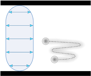
Consider the flow configuration illustrated in figure 1(a). A neutrally buoyant spherical particle of radius  $a$ is suspended in a Newtonian liquid of kinematic viscosity $\nu$ as it flows through a 2-D channel of width $l$ at a distance $d$ from the wall. The underlying flow in the channel is pulsatile and consists of a weak steady flow component $\bar {\boldsymbol {u}}'(z')$ with centreline velocity $\bar {u}'_s$ and a strong oscillatory flow component $\tilde {\boldsymbol {u}}'(z',t')$ with centreline displacement amplitude $s$ and angular frequency $\omega$. The origin of the coordinate system is taken at the centre of the particle.

Figure 1. (a) Idealized illustration of inertial focusing in planar pulsatile flows between parallel plates. A spherical particle of radius  $a$ is suspended in a pulsatile flow, composed of a steady ( $\bar {\boldsymbol {u}}'(z'$)) and an oscillatory ( $\tilde {\boldsymbol {u}}'(z',t'$)) component. (b) Analytical results, (3.18) and (3.19), of the migration velocity profile along the channel width for different Womersley number pulsatile flows.
The relevant non-dimensional numbers are the relative particle size  $\kappa =a/l$, the Strouhal number ${St}=l/s$ and the relative magnitude of the steady flow $\bar {u}'_s/s\omega$. Of primary interest are the channel Womersley number, $\alpha =l\sqrt {\omega /\nu }$, which is a relative measure of the unsteady inertial force to the viscous force, and the particle Reynolds number, ${Re}_{{p}}=a^{2} s\omega /l\nu =\kappa ^{2} \alpha ^{2}/ {St}$, which quantifies the ratio of the particle's lateral migration velocity to its disturbance velocity. The Reynolds number ( ${Re} = s \omega l / \nu = \alpha ^{2}/{St}$) quantifies the inertial to viscous forces at the channel scale. It determines focusing position in steady flows, particularly when ${Re} > 15$ (Segré & Silberberg Reference Segré and Silberberg1961; Schonberg & Hinch Reference Schonberg and Hinch1989). Here, the isolated effect of oscillatory flow is studied by maintaining ${Re} < 10$ and varying $\alpha$. As will be demonstrated, both ${Re}$ and ${Re}_{{p}}$ are insufficient for describing oscillatory flow focusing. Instead ${St}$ and $\alpha$ must be considered separately, since they result in qualitatively different effects, especially if $\alpha >5$.
3. Asymptotic analysis
The treatment here is for a small particle ( ${Re}_{p}\ll 1$ and $a/l\ll 1$) in a steady 2-D channel flow (Schonberg & Hinch Reference Schonberg and Hinch1989) and is extended to the case of a harmonic purely oscillatory flow. For a particle with a certain translation velocity ${\boldsymbol {U}}_{{p}}'$ and angular velocity $\boldsymbol {\varOmega }_{{p}}'$, the governing equations in terms of the position ${\boldsymbol {r}}'$, time $t'$, disturbance velocity $\boldsymbol {u}'$ and disturbance pressure $p'$ are
 $$\begin{gather} \boldsymbol{\nabla}'\boldsymbol{\cdot} {\boldsymbol{u}}'=0, \end{gather}$$
 $$\begin{gather}\nu {\nabla'}^{2}{\boldsymbol{u}}'-\frac{1}{\rho}\boldsymbol{\nabla}'p'={\partial_{t'} {\boldsymbol{u}}'}+{\tilde{{\boldsymbol{u}}}}'\boldsymbol{\cdot}\boldsymbol{\nabla}'{\boldsymbol{u}}'+ {\boldsymbol{u}}'\boldsymbol{\cdot}\boldsymbol{\nabla}'{\tilde{{\boldsymbol{u}}}}' +{\boldsymbol{u}}'\boldsymbol{\cdot}\boldsymbol{\nabla}' {{{\boldsymbol{u}}}}'+{\boldsymbol{U}}_{ {p}}' \boldsymbol{\cdot} \boldsymbol{\nabla}' {\tilde{{\boldsymbol{u}}}}'. \end{gather}$$
 The undisturbed velocity is  ${\tilde {\boldsymbol {u}}}'=s\omega ({\tilde {u}} \textrm {e}^{\textrm {i}\omega {t'}}+{\tilde {u}}^{*} \textrm {e}^{-\textrm {i}\omega {t'}})\boldsymbol {e}_{{x}}$, where ${\tilde {u}}$ and its complex conjugate $\tilde {u}^{*}$ are obtained by applying
 ![]() and
and ![]() to the standard pulsatile flow profile for walls at
to the standard pulsatile flow profile for walls at ![]() :
:
 \begin{equation} \tilde{u}^{{{\dagger}}} = \frac{\cosh{(\sqrt{\textrm{i}}\,\alpha {\breve{z}}'/l)} -\cosh{(\sqrt{\textrm{i}}\,\alpha/2)}}{2(1-\cosh{(\sqrt{\textrm{i}}\,\alpha/2)})}. \end{equation}
The transformations arise from placing the origin on a particle moving with the flow at a distance  $d/l$ from the channel wall, leading to
 \begin{equation} \tilde{u} = \frac{\sinh{(\sqrt{\textrm{i}}\,\alpha z'/2l)}\sinh{(\sqrt{\textrm{i}} \,\alpha (z'+2d-l)/2l)}}{1-\cosh{(\sqrt{\textrm{i}}\,\alpha/2)}}. \end{equation}
The above equations are subject to a no-slip condition at the particle surface and the channel walls as well as regularity at the far field. That is,  $\boldsymbol {u}'={\boldsymbol {U}}_{{p}}'+\boldsymbol {\varOmega }_{{p}}' \times {\boldsymbol {r}}'-\tilde {\boldsymbol {u}}'$ on $r'=a$, $\boldsymbol {u}'=0$ on $z'=l$ and $z'=l-d$, and finally $\boldsymbol {u}'\rightarrow 0$ as $x'\rightarrow \infty$, respectively.
3.1. Inner problem
For the inner problem, the dimensionless position, time and rate of strain are defined as  $\boldsymbol {r}=\boldsymbol {r}'/a$, $t= t' \omega$ and $\gamma =\gamma '(l/s\omega )$, respectively. The corresponding rescaled pressure and velocities are $p=p'(l/\rho \nu s \omega )$, $\boldsymbol {u}=\boldsymbol {u}'(l/{s\omega a})$, $\boldsymbol {U}_{{p}}=\boldsymbol {U}_{{p}}'(l/s\omega a)$ and $\boldsymbol {\varOmega }_{p}=\boldsymbol {\varOmega }'_{p} (l/s\omega )$. The undisturbed velocity is approximated by an oscillatory simple shear flow ( ${\tilde {\boldsymbol {u}}}_{I}=\gamma z \textrm {e}^{\textrm {i}t}\boldsymbol {e}_{{x}} + \gamma ^{*} z \textrm {e}^{-\textrm {i}t}\boldsymbol {e}_{{x}}$), where
 \begin{equation} \gamma=\frac{\sqrt{\textrm{i}}\,\alpha}{2} \frac{\sinh{(\sqrt{\textrm{i}} \,\alpha(2d-l)/2l)}}{1-\cosh{(\sqrt{\textrm{i}}\,\alpha/2)}}. \end{equation}
The momentum equations become
 \begin{equation} {\nabla^{2}}\boldsymbol{u}-\boldsymbol{\nabla} p= {Re}_{{p}} ({St}\,{\partial_t \boldsymbol{u}}+{\tilde{\boldsymbol{u}}_{{I}}}\boldsymbol{\cdot}\boldsymbol{\nabla} \boldsymbol{u}+\boldsymbol{u}\boldsymbol{\cdot}\boldsymbol{\nabla}{\tilde{\boldsymbol{u}}_{{I}}} +\boldsymbol{u}\boldsymbol{\cdot}\boldsymbol{\nabla} {{\boldsymbol{u}}}+\boldsymbol{U}_{{p}} \boldsymbol{\cdot} \boldsymbol{\nabla} {\tilde{\boldsymbol{u}}_{{I}}}).\end{equation}
The boundary conditions for the inner problem are  $\boldsymbol {u}={\boldsymbol {U}}_{{p}}+\boldsymbol {\varOmega }_{{p}} \times \boldsymbol {r}-\tilde {\boldsymbol {u}}_{{I}}\ \textrm {on}\ r=1$ and $\boldsymbol {u}\rightarrow 0 \textrm { as } r\rightarrow \infty .$ The unsteady term is significant at leading order only if ${Re}_{p}{St}>1$. Since this is not the case in experiments, this term is neglected, and the equations are identical to those of the inner problem in Schonberg & Hinch (Reference Schonberg and Hinch1989). Consequently, the inner problem is quasi-steady, and unsteadiness at the channel scale manifests at the particle scale only through the local shear rate. The solution at the far field ( $r\rightarrow \infty$) is
 \begin{equation} \boldsymbol{u}={-}\frac{5}{2}(\gamma\textrm{e}^{\textrm{i}t}+\gamma{}^{*}\textrm{e}^{-\textrm{i}t}) \frac{\boldsymbol{r}xz}{r^{5}} + O(r^{{-}3}). \end{equation}
3.2. Outer problem
For the outer problem, the dimensionless time and rate of strain are the same as before, while the position is defined as  $\boldsymbol {R}=\boldsymbol {r}'/l$. Dimensionalizing (3.7) and rescaling the coordinates with $l$, we find that the asymptotic matching condition for the disturbance velocity implies that $\boldsymbol {u}'\sim \kappa ^{3} s\omega$ as $R\rightarrow 0$. It therefore follows that $\boldsymbol {U}=\boldsymbol {u}'/(\kappa ^{3} s\omega )$, $\tilde {\boldsymbol {U}}=\tilde {\boldsymbol {u}}'/(s\omega )$ and ${P}=p'(l/\rho \nu s \omega \kappa ^{3})$. The rescaled momentum equation is
 \begin{align} &{\nabla^{2}}\boldsymbol{U}-\boldsymbol{\nabla} {P}-\alpha^{2}{\partial_t \boldsymbol{U}} \nonumber\\ &\quad = {Re}({\tilde{\boldsymbol{U}}}\boldsymbol{\cdot}\boldsymbol{\nabla}\boldsymbol{U}+ \boldsymbol{U}\boldsymbol{\cdot}\boldsymbol{\nabla}{\tilde{\boldsymbol{U}}}) +\frac{10{\rm \pi}}{3}(\gamma \textrm{e}^{\textrm{i}t}+\gamma^{*} \textrm{e}^{-\textrm{i}t}) (\boldsymbol{e}_{{x}}{\partial_Z} +\boldsymbol{e}_{{z}}{\partial_X} )\delta_{\boldsymbol{R}}, \end{align}
subject to  $\boldsymbol {U}=0$ at $Z=-d/l$ and $Z=1-d/l$ as well as $\boldsymbol {U}\rightarrow 0 \textrm { as }X\rightarrow \infty .$
The last term on the right-hand side of (3.8) is the singularity at  $R=0$ due to the particle. The contributions of $\boldsymbol {u}'\boldsymbol {\cdot }\boldsymbol {\nabla }' {{\boldsymbol {u}}}'$ and $\boldsymbol {U}_{{p}}' \boldsymbol {\cdot } \boldsymbol {\nabla }' {\tilde {\boldsymbol {u}}}'$ are less than the remaining terms by a factor of at least $\kappa ^{2}$ and are hence neglected at this order. The equations for a steady flow can be recovered setting $t=0$ and $\alpha \rightarrow 0$ throughout.
In order to proceed, it is necessary to decouple the time-dependent forcing in (3.8) from the inertial terms for tractability. To do this, a simplifying assumption that  $\kappa ^{2}\ll Re\ll 1$ is made. Although $Re\sim 10$ for our experiments, the assumption is not thought to affect comparison with experiments. This is suggested by the steady flow case, where results derived assuming $Re\ll 1$ in Ho & Leal (Reference Ho and Leal1974) are valid at least till $Re=15$. Next, we choose the following ansatz for $\boldsymbol {U}$ and ${P}$:
 \begin{equation} \left.\begin{gathered} \boldsymbol{U}=\boldsymbol{U}_0\textrm{e}^{\textrm{i}t}+\boldsymbol{U}^{*}_0 \textrm{e}^{-\textrm{i}t}+Re(\boldsymbol{U}_{1s}+\boldsymbol{U}_1\textrm{e}^{\textrm{i}2t}+ \boldsymbol{U}^{*}_1\textrm{e}^{-\textrm{i}2t})+Re^{2}(\dots),\\ {P}={P}_0\textrm{e}^{\textrm{i}t}+{P}^{*}_0\textrm{e}^{-\textrm{i}t}+Re({P}_{1s}+{P}_1\textrm{e}^{\textrm{i}2t}+ P_1^{*}\textrm{e}^{-\textrm{i}2t})+Re^{2}(\dots). \end{gathered}\right\} \end{equation}
With the above, the time dependence of  $\boldsymbol {U}$ and ${P}$ has been made explicit. That is, all the newly defined $\boldsymbol {U}_i$ and ${P}_i$ terms are independent of time. This implies that only $\boldsymbol {U}_{1s}$ and ${P}_{1s}$ are relevant to long-term particle migration, with the rest averaging out to zero over a single oscillation cycle. The ultimate objective is therefore the evaluation of $\boldsymbol {U}_{1s}({0})\boldsymbol {\cdot }\boldsymbol {e}_{{z}}$, which directly yields the particle migration velocity in the laboratory frame. The oscillatory nature of forcing, however, requires $\boldsymbol {U}_{0}$ and ${P}_{0}$ to be evaluated first. Substituting the ansatz in (3.8), the $O(1)$ terms give
 $$\begin{gather} ({\nabla^{2}}-\textrm{i}\alpha^{2})\boldsymbol{U}_0-\boldsymbol{\nabla} P_0=\frac{10{\rm \pi}}{3}\gamma(\boldsymbol{e}_{{x}}{\partial_Z} +\boldsymbol{e}_{{z}} {\partial_X} )\delta_{\boldsymbol{R}}, \end{gather}$$
 $$\begin{gather}{\nabla^{2}}{P}_0={-}\frac{20{\rm \pi}}{3}\gamma{\partial_X\partial_Z\delta_{\boldsymbol{R}}}. \end{gather}$$
The above system of partial differential equations are converted into a system of ordinary differential equations through a Fourier transformation defined as
 \begin{equation} \hat{\boldsymbol{U}}_0(k_1,k_2,Z)=\frac{1}{4{\rm \pi}^{2}}\int_{-\infty}^{\infty} \int_{-\infty}^{\infty}\boldsymbol{U}_0 \exp({-\textrm{i}(k_1X+k_2Y)})\,\textrm{d}X\,\textrm{d}Y. \end{equation}
 To obtain cross-stream migration, it is sufficient to consider only the  $Z$ component ${W}_0=\boldsymbol {U}_{{0}}\boldsymbol {\cdot }\boldsymbol {e}_{{z}}$. Equations (3.10) and (3.11) in Fourier space are therefore
 $$\begin{gather} ({d}^{2}_Z-k^{2}-\textrm{i}\alpha^{2})\hat{{W}}_0- {{d}_Z\hat{{P}}_0}=0, \end{gather}$$
 $$\begin{gather}({d}^{2}_Z-k^{2})\hat{{P}}_0=0, \end{gather}$$
where  $k^{2}=k_1^{2}+k_2^{2}$. The boundary conditions are $\hat {{W}}_0=0$ and ${d}_Z \hat {{W}}_{0}=0$ at $Z=-d/l$ and $Z=1-d/l$. The condition at $Z=0$ is written as
 \begin{equation} \left(\hat{{P}}_{0}\quad {d}_Z\hat{{P}}_{0}\quad \hat{{W}}_{0}\quad {d}_Z\hat{{W}}_{0}\right)^{0^{+}}_{0^{-}} = \frac{5}{6{\rm \pi}}\textrm{i} k_1\gamma \left(2\quad 0\quad 0\quad 1 \right). \end{equation}
To obtain the equations for  $\boldsymbol {U}_{1s}$, the $O({Re})$ terms obtained by substituting the ansatz in (3.8) are gathered and averaged over a single time period. The resulting equation and its divergence are
 $$\begin{gather} {\nabla^{2}}\boldsymbol{U}_{1s}-\boldsymbol{\nabla} {P}_{1s}= ({W}_0\partial_Z{\tilde{U}^{*}}+{W}_0^{*}\partial_Z{\tilde{U}})\boldsymbol{e}_{{x}}+ (\tilde{U}^{*}\partial_X{\boldsymbol{U}_0}+\tilde{U}\partial_X{\boldsymbol{U}^{*}_0}), \end{gather}$$
 $$\begin{gather}{\nabla^{2}}P_{1s}={-}2(\partial_X{{W}_0}\partial_Z{\tilde{U}^{*}}+ \partial_X{{W}_0^{*}}\partial_Z{\tilde{U}}). \end{gather}$$
The Fourier transforms of the above equations give
 $$\begin{gather} ({d}^{2}_Z-k^{2})\hat{{W}}_{1s}-{{d}_Z\hat{{P}}_{1s}}=\textrm{i}k_1( \hat{{W}}_{0}{\tilde{U}^{*}}-\hat{{W}}_{0}^{*}{\tilde{U}}), \end{gather}$$
 $$\begin{gather}({d}^{2}_Z-k^{2})\hat{{P}}_{1s}={-}2\textrm{i} k_1(\hat{{W}}_{0}{d}_Z{\tilde{U}^{*}}-\hat{{W}}^{*}_{0}{d}_Z{\tilde{U}}). \end{gather}$$
Note that forcing occurs due to  $O(1)$ solutions interacting with the undisturbed flow. At this order, the boundary conditions at $Z=-d/l$ and $Z=1-d/l$ are $\hat {{W}}_{1s}=0$ and ${d}_Z \hat {{W}}_{1s}=0$. At $Z=0$, $\hat {{P}}_{1s}$ and $\hat {{W}}_{1s}$ along with the corresponding first derivatives are continuous.
3.3. Evaluation of the migration velocity profile
From the exact solutions to (3.13), (3.14), (3.18) and (3.19), the lateral migration velocity can be synthesized numerically using
 \begin{equation} {{W}}_{{p}}={{W}}_{1s}(0)=\int_{-\infty}^{\infty}\int_{-\infty}^{\infty} \hat{{W}}_{1s}(0,k_1,k_2)\,\textrm{d}k_2\,\textrm{d}k_1. \end{equation}
Since  $\hat {{W}}_{1s}$ is even in both $k_1$ and $k_2$, the integration can be limited to the first quadrant so long as the result is multiplied by a factor of 4. To assist convergence of the integral, the analytical solution for $k\gg 1$ was used:
 \begin{equation} \hat{{W}}_{1s}(0) = \frac{15 k_1^{2}\alpha^{2} }{64{\rm \pi} k^{5}} \, \textrm{Re}\left[\frac{\textrm{i} \gamma\cosh({\textrm{i}^{3/2}{\alpha}(d/l-1/2)})} {\cosh({\textrm{i}{}^{3/2}{\alpha}/2})-1}\right], \end{equation}
where  $\textrm {Re}$ denotes the real part.
The variation of the particle migration velocity  ${{W}}_{{p}}$ with $d/l$ for different values of the Womersley number is shown in figure 1(b). For small Womersley numbers ( $\alpha \leqslant 5$), the migration velocity profiles are very similar to one another and, more importantly, nearly identical to the migration profile expected for steady flow, within a numerical factor of exactly 1/2 (Asmolov Reference Asmolov1999). The factor of 1/2 arises from the time average of the $\cos ^{2}{t}$ term over a single oscillation period. For large Womersley numbers ( $\alpha >5$), the migration velocity increases near the channel walls ( $d/l < 0.1$) and becomes negligible in the central region of the channel ( $0.2 < d/l < 0.5$). The equilibrium focusing position can be located by determining the null point for each of the migration velocity profiles. The value $\alpha =5$ is straightforward given that the undisturbed velocity profile (3.3) changes dramatically beyond this threshold. Less so is the null point, which moves closer to the wall with increasing $\alpha$ as a result of opposing effects (see figure 3a). Owing to increasing $\alpha$, velocity gradients become larger near the walls and smaller near the centreline (3.3). This implies that the wall interaction force becomes relatively stronger but is also confined closer to the wall. Note that results in figure 1(b) are not valid for $d/l\rightarrow 0$ and break down when $d/l\sim \kappa$, as this violates the assumed separation of scales between the outer and inner problems. The oscillatory flow-induced inertial lift on a sphere close to a wall has been addressed numerically by Fischer et al. (Reference Fischer, Leaf and Restrepo2004).
4. Experimental methods
Experiments were performed in a straight channel with a rectangular cross-section of high aspect ratio fabricated from a piece of aluminium sheet metal through wire electrical discharge machining. The total channel length  $L$ was $4$ cm and the height was $2.5$ mm. The channel walls were wet sanded to smoothness, resulting in a width $l$ of $300\ \mathrm {\mu }\textrm {m}$ with ${<}0.2\,\%$ deviation from parallel plates along the channel length. The top and bottom walls of the channel were completed by adhering transparent packaging tape to the sheet metal. The tape was perforated at the channel inlet and outlet, and microfluidic tubing was inserted and sealed with epoxy.
The variable-frequency pulsatile flow in the microfluidic device was generated by combining a steady flow component with an oscillatory flow component. The steady flow component was generated at the inlet using a syringe pump. A volumetric flow rate of  $20 \ \mathrm {\mu }\textrm {l}\ \min ^{-1}$ was used throughout this study unless specified otherwise. For the given channel dimensions, this flow rate corresponded to a maximum flow speed $\bar {u}'_s=0.54\ \textrm {mm}\ \textrm {s}^{-1}$. The oscillatory flow component was generated at the outlet using an oscillatory pressure signal generated by an external oscillatory driver. This was accomplished by interfacing the microfluidic tubing at the outlet to a loudspeaker diaphragm (Vishwanathan & Juarez Reference Vishwanathan and Juarez2020). The frequencies used here range over $25\leqslant f \leqslant 500$ Hz, with the angular frequency defined as $\omega = 2 {\rm \pi}f$. The maximum values of the oscillatory velocities ranged from $34$ to $89\ \textrm {mm}\ \textrm {s}^{-1}$ and were much larger than the steady flow velocity ( $s\omega \gg \bar {u}'_s$).
Polystyrene particles were density-matched in an aqueous glycerol solution ( $23\,\%$ w/w) with density $\rho =1060\ \textrm {kg}\ \textrm {m}^{-3}$ and kinematic viscosity $\nu =1.687\times 10^{-6}\ \textrm {m}^{2}\ \textrm {s}^{-1}$. Three different suspensions with particle radii $a=5.4$, 8.1 and $10.4\ \mathrm {\mu }\textrm {m}$ were used. Particle suspensions were in the dilute limit with volume fractions ranging from 0.02 % up to 0.05 %. Particles were imaged at the channel midplane (height) with bright-field microscopy using a $10\times$ objective lens with a depth of focus of $10 \ \mathrm {\mu }\textrm {m}$. The acquisition frequency of 5 Hz and exposure time of $100\ \mathrm {\mu }\textrm {s}$ were used to monitor the rectified component of particle displacement. The imaging location was at the lengthwise centre of the channel, or 2 cm away from the inlet. The residence time of a particle is defined as the shortest time to travel from the inlet to the region of observation and is given by $t_R=L/2\bar {u}'_s = 37$ s. However, during this time, the maximum total distance travelled by a particle will take into account the oscillatory component, since $s\omega \gg \bar {u}'_s$, and so it is estimated that $L_R= 4 s f t_R$. Therefore, here $L_R$ is referred to as the focusing distance travelled before observation and ranges from $0.8$ to $2.1$ m.
5. Experimental results
The dynamics of inertial focusing in planar pulsatile flows is qualitatively demonstrated in the space–time plot shown in figure 2(a). Here, suspended particle concentrations at each position along the channel width are represented in greyscale, where light grey corresponds to a low concentration of particles and dark grey corresponds to a high concentration of particles. Initially, particles are uniformly distributed along the spanwise direction, as they are transported by a purely steady unidirectional flow. After the oscillatory component is introduced ( $t=0$), concentration gradients emerge as particles migrate across streamlines and localize into two dark bands.

Figure 2. (a) Space–time plot of suspended particles migrating to equilibrium positions under pulsatile flow. (b) Histograms of the particle distribution along the channel width for (left) steady flow and (right) pulsatile flow. The focusing efficiency, denoted by  ${F}_{20}$, quantifies the fraction of particles found within a distance $l/10$ of both focusing positions. (c) Transient focusing efficiency for different steady flow velocities. The efficiency reaches a steady value for all cases after $t/t_R > 1.5$.
Histograms of particle positions along the channel width, obtained from digital particle identification and tracking techniques, quantitatively demonstrates the transformation from a uniformly dispersed suspension to a focused suspension, shown in figure 2(b). The particle number distributions are normalized by the total flux of particles observed. The peaks of the distribution correspond to the localization of particles after migration across streamlines. The peak positions are the measured equilibrium focusing positions, defined by their distance  $d_f/l$ from the channel walls. Since this measurement depends on the local width of the channel, particle tracking was used to extract the steady flow profile that was then fitted to a parabolic curve, whose fitting constants determine the precise centreline and local channel width. The focusing efficiency, denoted by ${F}_{20}$, quantifies the total fraction of particles located within a distance $l/10$ of both focusing positions and is indicated by the shaded band shown in figure 2(b). Therefore, ${F}_{20}$ ranges from $20\,\%$, corresponding to a uniformly dispersed suspension, up to $100\,\%$, corresponding to the complete localization of particles at the focusing positions.
When observing a fixed position along the channel length, the steady flow component determines both the absolute time required for the particle distribution to reach steady state and the eventual focusing efficiency. For example, the focusing efficiency for  $\alpha =4$, $\kappa =0.018$, ${Re}_{{p}}=0.014$ and the steady flow speeds $\bar {u}'_s$ of $0.27$, $0.52$ and $1.04\ \textrm {mm}\ \textrm {s}^{-1}$ initially starts from $20\,\%$ and increases with time, as shown in figure 2(c). The residence times $t_R$ associated with the steady flow speeds are $74$,
$74$,  $37$ and $18.5$ s, respectively. The rate of increase in the focusing efficiency is initially identical for all steady flow speeds and approaches zero by $t/t_R=1.5$. As expected, the steady state ${F}_{20}$ increases with residence time due to the larger focusing length travelled and reaches maximum values of $50\,\%$, $45\,\%$ and $40\,\%$, respectively.
The focusing positions and focusing efficiency are measured only after the particle distributions reach a steady state. Henceforth, the data presented will correspond to a steady state with a steady flow speed of  $\bar {u}'_s=0.54\ \textrm {mm}\ \textrm {s}^{-1}$ with a residence time of t R = 37 s. To ensure steady state, measurements are only made after pulsatile flow is applied for 100 s ( $t/t_R>2.5$), after which the particle distribution is measured and synthesized over another 100 s interval. The data (symbols) for focusing position and focusing efficiency are mean values (multiple experiments and time-averaged during the 100 s interval). The coloured regions represent the error, estimated here as half of the maximum difference of any measurement from the mean. For example, the comparison between instantaneous values and mean value are evident in figure 2(c).
The focusing positions  $d_f/l$ approach the channel wall as the Womersley number increases above $\alpha > 5$, as shown in figure 3(a). For small $\kappa$, there is good agreement between experimental measurements ( $\kappa < 0.02$) and theory ( $\kappa =0$), as indicated by the dashed line. The theoretical focusing positions are determined by null points in the migration velocity curves, shown in figure 1(b). For large $\kappa$, the deviation of experimental measurements ( $\kappa > 0.02$) from theory ( $\kappa =0$) increases with particle size. The corresponding focusing position for a given Womersley number occurs farther away from the channel wall, while preserving the qualitative theoretical ( $\kappa =0$) trend. That is, the focusing positions continue to approach the channel wall for Womersley numbers above $\alpha > 5$. While the focusing position can be described quite accurately with advanced computational methods for an individual particle, the evaluation of focusing efficiency requires a comprehensive statistical analysis of particle positions for many particles across all initial conditions. This is made possible only with an experimental approach.

Figure 3. (a) The focusing position for different relative particle sizes as a function of Womersley number. The experimental measurements (symbols) are similar to the analytical predictions (dashed) obtained from figure 1(b). The discrepancy is due to finite particle size ( $\kappa >0.02$). (b) The focusing efficiency for suspensions of different relative particle sizes as a function of Womersley number. The oscillatory velocity amplitude ( $s\omega$) is maintained constant across throughout. (c) The focusing efficiency for a suspension of a fixed particle size as a function of the Womersley number for varying oscillatory velocity amplitude. The oscillatory velocity amplitude is kept constant for a single curve but varied across curves. (d) The migration velocity profile for a low (blue) and high (red) Womersley number. The experimental measurements (symbols) are compared to corresponding theoretical results for point particles in an oscillatory flow (red solid and blue solid, (3.18) and (3.19)), as well as being compared to point (black dashed) and finite-size (grey stripe; Asmolov et al. Reference Asmolov, Dubov, Nizkaya, Harting and Vinogradova2018) particles in a steady flow.
The focusing efficiency was measured for different particle sizes and Womersley numbers, shown in figure 3(b). Here, the focusing length of  $L_R=2.1$ m was maintained across frequencies by independently adjusting the amplitude and frequency such that the product of the oscillatory velocity magnitude ( $s\omega$) is equal to a constant. For small Womersley numbers ( $\alpha < 5$), the focusing efficiency ranges from $50\,\%$ to $90\,\%$ for the particle Reynolds numbers of $0.01$ and $0.07$, respectively. The high extent of focusing efficiency, ${F}_{20} > 80\,\%$ for ${Re}_{{p}}=0.071$, illustrates the effectiveness of oscillatory flows for inertial focusing. For large Womersley numbers ( $\alpha > 5$), the focusing efficiency decreases monotonically and approaches $20\,\%$, or that of a uniformly dispersed suspension, for the smallest particle size.
The focusing efficiency was also measured for different oscillatory amplitudes and Womersley numbers, shown in figure 3(c). Here, the relative particle size of  $\kappa =0.035$ was maintained constant throughout. Once again, for small Womersley numbers ( $\alpha < 5$), the focusing efficiency has a similar range of $45\,\%$ to $90\,\%$ for the oscillatory velocities of $34$ and $89\ \textrm {mm}\ \textrm {s}^{-1}$, respectively. For large Womersley numbers ( $\alpha > 5$), the focusing efficiency decreases monotonically and approaches $20\,\%$ for the lowest oscillatory amplitude. From both cases, for a fixed Womersley number, a larger $s \omega$ or $\kappa$ value determined a higher extent in the ${F}_{20}$ value, in agreement with inertial focusing in steady flows.
A distinct advantage of studying inertial focusing in oscillatory flows compared to focusing in steady flows is that the migration of individual particles across a large resident path length can be clearly observed and tracked. Therefore, it is possible to accurately, measure the average migration velocity profile across the channel width, something that is not easily achieved in steady flows due to practical constraints of resolving single particles over a large field of view. The guiding principle is, once again, the decoupling of travelled distance from displacement (Vishwanathan & Juarez Reference Vishwanathan and Juarez2020). The averaged migration velocity at each spanwise position for a low-frequency ( $\alpha =3.2$) and a high-frequency ( $\alpha =7.8$) pulsatile flow and relative particle size of $\kappa =0.035$ is shown in figure 3(d). The migration velocity was measured by tracking the position of many individual particles ( $N \approx 100 - 1000$ per experiment) during the transient regime, i.e. $t/t_R < 1$ in figure 2(c). Experimental measurements (symbols) compare well with analytical results for point particles (solid, (3.18) and (3.19)) in an oscillatory flow. Here, symbols represent average values and error bars represent one standard deviation from the mean. A precise match with half the magnitude of numerical results for finite-sized particles (grey stripe, $\kappa =0.035$; Asmolov et al. Reference Asmolov, Dubov, Nizkaya, Harting and Vinogradova2018) in a steady flow is observed for the low-frequency case. See the comment about the numerical factor of 1/2 in § 3.3.
6. Discussion
The Womersley number is an important parameter for pulsatile flows (Dincau, Dressaire & Sauret Reference Dincau, Dressaire and Sauret2019). It defines the ratio of the channel width to the Stokes boundary layer thickness, and determines the velocity profile for unsteady laminar flows. While inertial focusing in pulsatile flows provides an opportunity for reduced channel lengths and pressure drops in biomedical applications, it first requires understanding the direct link between transient inertial forces and particle migration velocity profiles in unsteady laminar flows.
In general, the focusing efficiency is independent of  $\alpha$ for small Womersley numbers ( $\alpha < 5$), as shown in figures 3(b) and 3(c). The constant focusing efficiency for these cases is due to the migration velocity profiles, which are also independent for $0 < \alpha < 5$, as shown in figure 1(b). However, for large Womersley numbers ( $\alpha > 5$), the focusing efficiency decreased monotonically with increasing $\alpha$, as shown in figures 3(b) and 3(c). The decrease in the focusing efficiency for these cases is due to the migration velocity profiles, which become increasingly weak at the centre of the channel for $\alpha > 5$, as shown in figure 1(b).
For focusing in steady laminar flows, the particle Reynolds number determines the magnitude of the particle migration velocity, that is, a larger  ${Re}_{{p}}$ corresponds to increased focusing efficiency. In contrast, ${Re}_{{p}}=\kappa ^{2} \alpha ^{2}/ {St}$ does not always directly correlate with improved focusing efficiency in unsteady oscillatory flows. In fact, above a critical Womersley number ( $\alpha > 5$), the focusing efficiency decreases with increasing ${Re_p}$ if only $\alpha$ is increased. Therefore, for the purposes of inertial particle focusing, it is best to maintain $\alpha <5$. For $\alpha > 5$, although the focusing efficiency decreases, the migration velocity profile suggests that particles migrate away from the channel wall with speeds that increase directly with Womersley number. This effect could be leveraged in efforts to mitigate the fouling of surfaces without affecting the bulk concentration profile.
Acknowledgements
We thank M. Garcia, I.C. Christov and G.J. Elfring for critical discussions and feedback on initial versions of this paper.
Acknowledgements
The authors report no conflict of interest.


 Open access