


1. Introduction
Rapidly rotating confined flows are encountered extensively in nature as well as in many engineering applications. The Coriolis effect in such flows acts as a strong restoring force against perturbations away from solid-body rotation, with responses to low-amplitude external perturbations dominated by inertial oscillations (Greenspan Reference Greenspan1968). These responses generally take the form of circularly polarised inertial waves, which are maximally helical with their velocity and vorticity vectors aligned (Davidson Reference Davidson2013). Their dispersion relation relates their frequency and direction of propagation, but says nothing about the magnitude of the associated wavevector. This results in peculiar laws of reflections at solid walls, where the wavelength may change upon reflection, depending on the wall orientation with respect to the rotation axis (Phillips Reference Phillips1963). Multiple reflections may lead to focusing, resulting in an increase in wavenumber and energy density, as well as to the wave energy converging to vertices or edges of the container (Greenspan Reference Greenspan1969) or onto thin attractor regions in the interior of the container (Maas Reference Maas2005; Sibgatullin & Ermanyuk Reference Sibgatullin and Ermanyuk2019).
The origin of these inertial waves is tied to the nature of the forcing. In the weakly viscous regime (quantified by Ekman number  ${E}\ll 1$), small-amplitude (quantified by Rossby number
  ${Ro}\ll 1$) parametric forcing, such as libration, leads to the formation of oscillatory boundary layers on the container walls that tend to emit wave beams into the interior from certain edges and vertices, or, if the container wall is smooth and continuously curved, from points or lines of critical slope, where the wall normal is locally orthogonal to the wave beam's group velocity (Hollerbach & Kerswell Reference Hollerbach and Kerswell1995; Kerswell Reference Kerswell1995).
An analogy is often drawn between inertial waves in rotating fluids and internal waves in stably stratified fluids, mainly because both systems result in similar dispersion relations. In stably stratified flows, buoyancy is the restoring force, and the stratification gradient direction plays the role of the axis of rotation. For internal waves, which are planar with their velocity and vorticity vectors orthogonal so that their helicity density is identically zero, a quasi-two-dimensional (quasi-2-D) approximation can generally be made. Detailed comparisons with experiments in an elongated container with a trapezoidal cross-section and simulations of the Navier–Stokes–Boussinesq equations in the same three-dimensional (3-D) geometry show excellent agreement on the details of internal wave attractors and their near invariance in the elongated direction for forcing amplitudes small enough to avoid instabilities (Brouzet et al. Reference Brouzet, Sibgatullin, Scolan, Ermanyuk and Dauxois2016). In rotating axisymmetric geometries subjected to small-amplitude axisymmetric body forces, the flow is independent of the azimuthal direction and depends only on two spatial coordinates, but all components of the velocity and vorticity vectors are non-zero, and the flows are intrinsically 3-D (Boury et al. Reference Boury, Sibgatullin, Ermanyuk, Shmakova, Odier, Joubaud, Maas and Dauxois2021). Various attempts have been made to study non-axisymmetric configurations that are invariant and unbounded in one direction, both numerically and theoretically using a quasi-2-D setting with a three-component velocity field (Jouve & Ogilvie Reference Jouve and Ogilvie2014), and experimentally in elongated containers with a trapezoidal cross-section (Manders & Maas Reference Manders and Maas2003). However, such a quasi-2-D approximation is generally not valid for inertial waves (Maas Reference Maas2005), and the fate of inertial waves and attractors is not a priori clear in fully enclosed non-axisymmetric 3-D containers (Maas Reference Maas2001).
The fate of inertial waves is often explored in the linear ( ${Ro}=0$) inviscid (
 ${E}=0$) regime via ray tracing (Maas Reference Maas2005). The linear inviscid vertex and edge beam analysis (VEBA) presented in Welfert, Lopez & Wu (Reference Welfert, Lopez and Wu2023) determined the possible outcomes of the ray tracing of beams emitted from active vertices and edges in a cuboid librating about an axis passing through the midpoints of two opposite edges. Depending on the aspect ratio of the cuboid and the librational frequency, the energy of a single beam either focuses onto an edge orthogonal to the rotation axis (a point attractor) or a closed circuit in a plane parallel to the rotation axis (interior attractor), or reflects from one edge to another and back without focusing or defocusing for isolated values of the frequency (a retracing state when viewed from a direction orthogonal to the walls parallel to the axis of rotation).
The nature of the forcing is typically not accounted for in theoretical (linear inviscid) studies of wave attractors. The forcing (and the viscous terms) impose additional constraints on the inertial response via symmetries. To determine how robust the linear inviscid VEBA results are in light of this requires either direct numerical simulations or experiments. Experiments typically have relatively large forcing amplitudes, resulting in (additional) nonlinear effects. The resulting nonlinearities lead to a myriad of effects, including triadic resonances, shear layer instabilities and geostrophic shears (Kerswell Reference Kerswell1999; Wu, Welfert & Lopez Reference Wu, Welfert and Lopez2020a; Lopez et al. Reference Lopez, Shen, Welfert and Wu2022).
The attractors in the linear inviscid setting are singular distributions. Viscosity regularises them, but it also dampens the inertial response to the extent that if the system is not forced continuously, then it evolves to solid-body rotation (at which point there are no singularities). In many theoretical studies (Rieutord & Valdettaro Reference Rieutord and Valdettaro1997, Reference Rieutord and Valdettaro2010, Reference Rieutord and Valdettaro2018; Rieutord, Georgeot & Valdettaro Reference Rieutord, Georgeot and Valdettaro2001; Rieutord, Valdettaro & Georgeot Reference Rieutord, Valdettaro and Georgeot2002; Ogilvie Reference Ogilvie2009; Le Dizès & Le Bars Reference Le Dizès and Le Bars2017; Lin & Ogilvie Reference Lin and Ogilvie2021; He et al. Reference He, Favier, Rieutord and Le Dizès2022; Lin et al. Reference Lin, Hollerbach, Noir and Vantieghem2023), it is assumed that either forcing is of such small amplitude ( ${Ro}\ll 1$) that the nonlinear advection term
  $(\boldsymbol {u}\boldsymbol {\cdot }\boldsymbol {\nabla })\boldsymbol {u}$ can be neglected, or the forced response is a single monochromatic circularly polarised wave for which
  $(\boldsymbol {u}\boldsymbol {\cdot }\boldsymbol {\nabla })\boldsymbol {u}$ vanishes identically in open space as a result of incompressibility. This is not the case in a finite container, where waves necessarily interact nonlinearly with other waves of different wavevector orientations emitted from other sites, or with the various reflections, including their own reflections. Small
  ${Ro}$ means small
  $|\boldsymbol {u}|$, but not necessarily small spatial gradients of
  $\boldsymbol {u}$, especially when focusing takes place. In practice, it is unclear whether or not
  $(\boldsymbol {u}\boldsymbol {\cdot }\boldsymbol {\nabla })\boldsymbol {u}$ remains bounded away from zero as
  ${Ro}\to 0$. This is all exacerbated by taking
  ${E}\ll 1$. While this generally implies reduced viscous effects, small
  ${E}$ results in thin but intense boundary layers, and internal shear layers in which spatial gradients are large so that
  $(\boldsymbol {u}\boldsymbol {\cdot }\boldsymbol {\nabla })\boldsymbol {u}$ and
  ${\nabla }^2 \boldsymbol {u}$ are not negligible.
The aim of the present study is to determine how robust the VEBA predictions described in Welfert et al. (Reference Welfert, Lopez and Wu2023) are when  $0<{E}={Ro}\ll 1$ using direct numerical simulations (DNS) of the full 3-D nonlinear Navier–Stokes equations, including the time-periodic forcing and no-slip boundary conditions. In the librating cube, the focusing to edges predicted by VEBA was confirmed in Wu, Welfert & Lopez (Reference Wu, Welfert and Lopez2022b) for all inertial forcing frequencies and sufficiently small
  ${E}={Ro}\lesssim 10^{-3}$. However, the DNS also revealed flow dynamics not predicted by VEBA, which were found to persist even as
  ${E}={Ro}\to 0$;
  ${E}={Ro}= 10^{-8}$ were the smallest values considered numerically. Nonlinear and viscous effects, which are neglected in VEBA, may not be small in the DNS even as
  ${E}={Ro}\to 0$. Here, we extend the study from the cube to the cuboid, for which interior attractors do exist.
2. Governing equations
A cuboid with square cross-section of side length  $L$ and height
  ${A{\kern-4pt}R} L$, where
  ${A{\kern-4pt}R}$ is the height-to-base aspect ratio, is completely filled with an incompressible fluid of kinematic viscosity
  $\nu$. The container is rotating around an axis passing through its centre and the midpoints of opposite horizontal edges at a mean rate
  $\varOmega$ that is modulated harmonically at a frequency
  $\sigma$ with amplitude
  $\delta \varOmega$. The system is non-dimensionalised using
  $L$ as the length scale and
  $1/\varOmega$ as the time scale, and is described in terms of a non-dimensional Cartesian coordinate system
  $\boldsymbol {x}=(x,y,z)\in [-0.5,0.5]^2\times [-0.5{A{\kern-4pt}R},0.5{A{\kern-4pt}R} ]$ that is fixed in the container, with the origin at the centre. The corresponding non-dimensional velocity field is
  $\boldsymbol {u}=(u,v,w)$. In these coordinates, the non-dimensional angular velocity is
 \begin{equation} \boldsymbol{\varOmega}(t)=[1+{Ro} \cos(2\omega t)] {\boldsymbol{\varOmega}_0}, \quad {\boldsymbol{\varOmega}_0}=(0,1,{A{\kern-4pt}R})/\sqrt{1+{A{\kern-4pt}R}^2}, \end{equation}
where  $2\omega =\sigma /\varOmega >0$ is the non-dimensional libration frequency, and the relative amplitude
  ${Ro}=\delta \varOmega /\varOmega$ is the Rossby number. Figure 1 shows a schematic of the system for the three aspect ratios
  ${A{\kern-4pt}R} =1/2$, 1 and 2 considered in the DNS. The two walls of the container at
  $x=\pm 0.5$ are parallel to the axis of rotation. The four remaining walls are inclined at angles
  $\alpha =\text {arccot}({A{\kern-4pt}R} ^{\pm 1})$ relative to the rotation axis
  $\boldsymbol {\varOmega }_0$. Four of the edges are orthogonal to
  $\boldsymbol {\varOmega }_0$; the two bisected by the rotation axis are termed the north and south polar edges, and the other two are the tropical edges. The remaining eight edges are inclined at angles
  ${\rm \pi} /2-\alpha$ relative to
  $\boldsymbol {\varOmega }_0$.

Figure 1. Schematic of the cuboid librating around its axis of rotation  $\boldsymbol {\varOmega }(t)$, for aspect ratios
  ${A{\kern-4pt}R}$ as indicated; the meridional plane
  $x=0$ is shown in blue.
The non-inertial frame of reference attached to the librating cuboid introduces Coriolis and Euler body forces into the (non-dimensional) governing equations:
 \begin{equation} \frac{\partial \boldsymbol{u}}{\partial t} +(\boldsymbol{u}\boldsymbol{\cdot}{\boldsymbol{\nabla}})\boldsymbol{u} +2\boldsymbol{\varOmega} \times \boldsymbol{u} + \frac{{\rm d} \boldsymbol{\varOmega}}{{\rm d} t} \times \boldsymbol{x}={-}{\boldsymbol{\nabla}}p +{E}\,{\nabla}^2\boldsymbol{u}, \quad {\boldsymbol{\nabla}}\boldsymbol{\cdot}\boldsymbol{u}=0, \end{equation}
where  ${E}=\nu /(\varOmega L^2)$ is the Ekman number, and
  $p$ is the reduced pressure that incorporates the centrifugal force. In this frame of reference, the no-slip boundary conditions are
  $\boldsymbol {u}=\boldsymbol {0}$ on all six walls of the container. For small but non-zero
  ${Ro}$, it is convenient to introduce
  $\boldsymbol {v}=\boldsymbol {u}/{Ro}$ and
  $p_r=p/{Ro}$, as in Lopez et al. (Reference Lopez, Shen, Welfert and Wu2022). Using (2.1a,b), the governing equations then become
 \begin{align} \frac{\partial \boldsymbol{v}}{\partial t} +{Ro}\,(\boldsymbol{v}\boldsymbol{\cdot}{\boldsymbol{\nabla}})\boldsymbol{v} +2\boldsymbol{\varOmega} \times \boldsymbol{v} - 2\omega\sin(2\omega t)\,\boldsymbol{\varOmega}_0 \times \boldsymbol{x}={-}{\boldsymbol{\nabla}}p_r +{E}\,{\nabla}^2\boldsymbol{v}, \quad {\boldsymbol{\nabla}}\boldsymbol{\cdot}\boldsymbol{v}=0. \end{align}
For  $0<{E}={Ro}\ll 1$, solutions
  $\boldsymbol {v}$ and
  $p_r$ of (2.3) are typically synchronous limit cycles that respect the centrosymmetry of the governing equations and boundary conditions,
 \begin{equation} \mathcal{C}: [\boldsymbol{v},p_r](\boldsymbol{x},t) \mapsto[-\boldsymbol{v},p_r](-\boldsymbol{x},t), \end{equation}
corresponding to a reflection through the origin. In the linear inviscid setting ( ${E}={Ro}=0$), the system (2.3) is formally reduced to a non-homogeneous linear system whose forcing is cognisant of the libration of the container, i.e. the Euler force persists.
The numerical scheme and code used here is essentially the same as that used in closely related problems (Lopez et al. Reference Lopez, Shen, Welfert and Wu2022; Wu et al. Reference Wu, Welfert and Lopez2022b). The governing equations (2.3) are discretised using a third-order linearly implicit scheme in time, and a spectral scheme in space. At each time step, the velocity components are updated via a third-order backwards difference formula scheme, with the viscous terms as well as the Coriolis and Euler forces treated implicitly, while the pressure gradient and nonlinear terms are evaluated via third-order extrapolation. This leads to a coupled system of elliptic equations with variable coefficients. The pressure is then updated via the solution of a Poisson problem posed in the cuboid, including the boundary, leading to a constant-coefficient Poisson equation. The number of time steps  $\delta t$ used per librational forcing period is
  $200$ for all Ekman and Rossby numbers considered here.
The elliptic and Poisson problems are discretised in each of the three spatial directions using Legendre polynomials of degree  $M$ for the velocity components, and degree
  $M-2$ for the pressure, with
  $M$ ranging from
  $M=100$ for
  ${E}=10^{-5}$ to
  $M=650$ for
  ${E}=10^{-8}$. Specifically, the velocity and pressure at times
  $t=n \delta t$ are expanded as
 \begin{equation} \boldsymbol{v}^n(x,y,z) = \sum_{i,j,k=2}^{M} a^n_{ijk}\,\psi_{ijk}(x,y,z), \quad p_r^n (x,y,z) = \sum_{i,j,k=0}^{M-2} b^n_{ijk}\,\psi_{ijk}(x,y,z), \end{equation}
in terms of basis functions
 \begin{equation} \psi_{ijk}(x,y,z) = \psi_i(2x)\,\psi_j(2y)\,\psi_k(2z/{A{\kern-4pt}R}), \end{equation}
with
 \begin{equation} \psi_i(\xi)=
r_i[\mathfrak{L}_{i-2}(\xi)-\mathfrak{L}_i(\xi)], \quad
i\ge0, \ {-1}\le\xi\le1,
\end{equation}
\begin{equation} \psi_i(\xi)=
r_i[\mathfrak{L}_{i-2}(\xi)-\mathfrak{L}_i(\xi)], \quad
i\ge0, \ {-1}\le\xi\le1,
\end{equation}
where  $\mathfrak {L}_k$ is the Legendre polynomial of degree
  $k$, with
  $\mathfrak {L}_k(\xi )=0$ for
  $k<0$, and normalising constants
  $r_i$. The property
  $\psi _i(\pm 1)=0$ for
  $i\ge 2$ guarantees
  $\boldsymbol {v}^n=\boldsymbol {0}$ on the walls of the cuboid, while the lower degree of
  $p_r^n$ compared to
  $\boldsymbol {v}^n$ guarantees the well-posedness of the resulting discrete problems. The resulting banded linear systems for the velocity and pressure updates are then diagonalised and solved. An optional scalar auxiliary variable procedure developed in Wu, Huang & Shen (Reference Wu, Huang and Shen2022a) introduces a third-order correction of the velocity that guarantees unconditional stability and improves the robustness of the scheme, in particular during transient dynamics.
3. Overview of ray tracing analysis
Ray tracing is normally performed on the unforced homogeneous system, neglecting the Euler force, but the forcing determines the locations from which beams are emitted. Viscous interactions between the oscillatory boundary layers driven by the small-amplitude librational forcing lead to inertial wave beams being emitted into the cuboid from vertices and/or edges. Which vertices and/or edges emit depends on  ${A{\kern-4pt}R}$ and
  $\omega$. In general, a vertex may emit along a double cone of directions with its apex at the emission point forming a conical sheet. However, a point on an edge may emit in only at most four directions because of continuity requirements with beams emitted from neighbouring points and tangentiality with conical sheets emitted from its endpoints, if any. The inviscid theory presented in Welfert et al. (Reference Welfert, Lopez and Wu2023) shows that a beam emitted from a vertex or an edge tends to be attracted, after many reflections, towards a plane with constant
  $x$, parallel to the axis of rotation. Ultimately, the beam focuses either onto a corner point in this planar cross-section, which is a point on an edge orthogonal to the axis of rotation, or onto a closed-loop interior attractor in this
  $x$-plane. In the inviscid setting, this
  $x$-plane depends non-smoothly on the location of the point or direction of emission because of boundary singularities (edges and vertices) creating jumps in the wall normal direction. However, in practice, these are regularised by viscous effects.
A closed-loop attractor is characterised by the number of reflections  $m$ at the wall
  $z=0.5{A{\kern-4pt}R}$ and
  $n$ at the wall
  $y=0.5$, with an equal number of reflections at walls
  $z=-0.5{A{\kern-4pt}R}$ and
  $y=-0.5$ by the centrosymmetry. Such an attractor is denoted
  $m:n$. Figure 2 shows the inviscid
  $(\omega ^2,{A{\kern-4pt}R} )$-regime diagram for wave beams contained completely in the meridional plane
  $x=0$. The region of existence of interior attractors is delimited by the curves
  $\omega ^2 = 1/(1+{A{\kern-4pt}R} ^{\pm 2})$, along which either the walls
  $y=\pm 0.5$ or the walls
  $z=\pm 0.5{A{\kern-4pt}R}$ have critical reflection slope. Inside this region, all reflections are supercritical, whereas outside the region, reflections on the walls at
  $y=\pm 0.5$ and
  $z=\pm 0.5{A{\kern-4pt}R}$ are subcritical. For
  ${A{\kern-4pt}R} =1$, reflections are not supercritical for any
  $\omega ^2$, and they are critical only for
  $\omega ^2=1/2$. Outside these regions, but for
  $\omega ^2<1$, inertial wave beams focus onto edges and/or vertices. For
  ${A{\kern-4pt}R} =1$, there are no interior attractors, and as
  $\omega ^2$ is varied across
  $1/2$, there is a switch in the edges and vertices to which wave beams focus. Note that in the limits
  ${A{\kern-4pt}R} ^{\pm 1}\to \infty$, the walls of the container tend to be either parallel or orthogonal to the rotation axis, yet the range of existence of interior attractors extends to
  $0<\omega ^2<1$.

Figure 2. Inviscid  $(\omega ^2,{A{\kern-4pt}R} )$-regime diagram for wave beams in the plane
  $x=0$: the bold black curves
  $\omega ^2=1/(1+{A{\kern-4pt}R} ^{\pm 2})$ delimit regions of differing criticality of wave beam reflections on the walls at
  $y=\pm 0.5$ or
  $z=\pm 0.5{A{\kern-4pt}R}$ and focusing of the beams onto
  $m:n$ or
  $n:m$ attractors. The red stars correspond to cases discussed in this study. The figure has been adapted from Welfert et al. (Reference Welfert, Lopez and Wu2023).
Although the attractors in a given  $x$-plane in the DNS and VEBA associated with
  ${A{\kern-4pt}R} =a$ and
  ${A{\kern-4pt}R} =1/a$ can be mapped to each other via a
  $90^\circ$ rotation and rescaling, other details differ away from the attractors due to conical shears originating from the vertices of the cuboids. These differences are due to the spanwise widths of the two configurations. A perfect match exists between the
  $1\times 1\times a$ and
  $1/a \times 1 \times 1/a$, rather than
  $1\times a\times 1/a$, configurations, albeit with a different effective Ekman number; see Appendix A for details.
4. Direct numerical simulations of simple attractors
We consider simple attractors, either a point attractor at edges for  ${A{\kern-4pt}R} =1$, or a 1 : 1 attractor for
  ${A{\kern-4pt}R} =1/2$ and
  ${A{\kern-4pt}R} =2$, all at the same libration frequency corresponding to
  $\omega =0.55$ (
 $\omega ^2=0.3025$); these cases are indicated by the red stars in figure 2. They are examined via DNS over the range
  ${E}={Ro}\in [10^{-8}, 10^{-5}]$. The spatial and temporal resolutions used for these DNS are listed in table 1. For all cases,
  ${E}$ and
  ${Ro}$ are sufficiently small that the responses to librational forcing are
  $\mathcal {C}$-invariant synchronous limit cycles. It is important to reduce both
  ${E}$ and
  ${Ro}$ in lock-step; fixing
  $0<{Ro}\ll 1$ and reducing only
  ${E}$ will lead to the fixed libration amplitude
  ${Ro}$ being sufficiently large for a sufficiently small
  ${E}$ to trigger flow instability. On the other hand, fixing
  $0<{E}\ll 1$ and reducing only
  ${Ro}$ ultimately results in a synchronous forced response flow whose magnitude
  $\|\boldsymbol {u}\|$ scales with
  ${Ro}$, so that
  $\|\boldsymbol {v}\|$ remains
  ${O}(1)$ and tends towards being temporally harmonic, corresponding to the solution of (2.3) with
  ${Ro}=0$. The interest in studying the response as both
  ${Ro}$ and
  ${E}$ are reduced in problems involving geometric focusing onto attractors is that even as
  ${Ro}$ is reduced, the gradients in the flow velocity grow as
  ${E}$ is reduced and the combined result is not a priori obvious.
Table 1. Degree  $M$ of the Legendre polynomials in each of the three spatial directions used in the DNS with
  $\omega =0.55$ and
  ${E}={Ro}$, and
  ${A{\kern-4pt}R}$ as indicated.

It is informative to put into perspective the ranges of  ${E}$ and
  ${Ro}$ considered here compared to current state-of-the-art laboratory experiments investigating inertial wave attractors (e.g. Brunet, Dauxois & Cortet Reference Brunet, Dauxois and Cortet2019; Boury et al. Reference Boury, Sibgatullin, Ermanyuk, Shmakova, Odier, Joubaud, Maas and Dauxois2021). The smallest Ekman numbers achieved experimentally are
 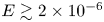 ${E}\gtrsim 2 \times 10^{-6}$, corresponding to a background rotation
  $\varOmega \approx 2\ {\rm rad}\ {\rm s}^{-1}$ in a container of length scale
  $L\approx 0.5$ m filled with water of kinematic viscosity
  $\nu \approx 10^{-6}\ {\rm m}^2\ {\rm s}^{-1}$. To achieve
  ${E}= 10^{-8}$ with water at the same background rotation rate, the container length scale needs to be
  $L\approx 7$ m. As for the Rossby number
  ${Ro}$ characterising the forcing amplitude in the experiments, this is no smaller than approximately
  $7 \times 10^{-3}$ due to signal-to-noise ratio issues; this is small enough for the flows to be strongly affected by the Coriolis force, but is nevertheless large enough to correspond to a developed nonlinear regime.
The flows are characterised primarily by using their enstrophy density  $\boldsymbol {\omega }^2=|\boldsymbol {\nabla }\times \boldsymbol {v}|^2$, its mean
 \begin{equation} \overline{\boldsymbol{\omega}^2}=\frac{1}{\tau} \int_{t^*}^{t^*+\tau} \boldsymbol{\omega}^2\, {\rm d} t, \end{equation}
and its standard deviation
 \begin{equation} \boldsymbol{\omega}^2_{SD} = \sqrt{\frac{1}{\tau} \int_{t^*}^{t^*+\tau} (\boldsymbol{\omega}^2-\overline{\boldsymbol{\omega}^2})^2\, {\rm d} t}, \end{equation}
where  $\tau ={\rm \pi} /\omega$ is the libration period, and
  $t^*$ is a time by which the response flow is
  $\tau$-periodic (typically of the order of
  $10^{3}\tau$).
At aspect ratios  ${A{\kern-4pt}R} =1/2$ and 2, in the limit with both
  ${E}\to 0$ and
  ${Ro}\to 0$,
  $1:1$ attractors exist in the range
  $\omega ^2\in (0.2,0.64)$ (Welfert et al. Reference Welfert, Lopez and Wu2023). Figure 3 illustrates these cases for
  $\omega =0.55$ and
  ${E}={Ro}\in [10^{-8}, 10^{-5}]$, along with the
  ${A{\kern-4pt}R} =1$ case for which focusing is to point attractors on the tropical edges. The figure shows
  $\overline {\boldsymbol {\omega }^2}$ and
  $\boldsymbol {\omega }^2_{SD}$ in the meridional plane
  $x=0$, seen from the positive
  $x$ direction, which summarise the synchronous response flow. Supplementary movie 1 animates
  $\boldsymbol {\omega }^2$ for the
  ${E}={Ro}= 10^{-8}$ cases over one libration period
  $\tau ={\rm \pi} /\omega$. For
  ${A{\kern-4pt}R} =1/2$ and 2, the traces of wave beams emanating from the four corners (the north and south poles and the midpoints of the tropical edges) focus onto an interior attractor that becomes thinner with deceasing
  ${E}$, while for
  ${A{\kern-4pt}R} =1$, the focusing is into the tropical corners. For all cases,
  $\overline {\boldsymbol {\omega }^2}$ and
  $\boldsymbol {\omega }^2_{SD}$ on the attractor seem to grow slightly faster than
  ${E}^{-1}$, while the response in the interior away from the attractor remains essentially independent of
  ${E}$ as
  ${E}$ is decreased. In the
  $x=0$ plane, VEBA of wave beams emitted from the four corners into the plane is also performed and compared to the DNS results. The VEBA in the last column of figure 3(a) captures well how the beams (depicted in blue) focus towards the attractor (depicted in red). Traces of the primary conic beams emitted from the vertices of the cuboid and of planar beams emitted from edges at
  $x=\pm 0.5$ intersecting the plane
  $x=0$ are also shown in light blue in the VEBA; these are also evident in the DNS. Secondary traces due to reflections of these beams, which are also visible in the DNS, are not included in VEBA (see Appendix B for further details concerning these beams).

Figure 3. (a) Mean enstrophy density  $\overline {\boldsymbol {\omega }^2}$ and (b) standard deviation of the enstrophy density
  $\sqrt {2}\boldsymbol {\omega }^2_{SD}$ in the meridional plane
  $x=0$ (where the rotation axis is vertical through the top and bottom corners), for
  ${A{\kern-4pt}R}$ and
  ${E}={Ro}$ as indicated. The last column in (a) has the VEBA results showing beams emitted from the four corners in blue and the attractor in red; traces of the primary conic beams emitted from the vertices of the cuboid and planar beams emitted from edges at
  $x=\pm 0.5$ are in light blue. Secondary traces due to reflections of these beams, which are visible in the DNS, are not included in VEBA. The black lines through the origin in panels in the first column of (a),
  $(0,y,0)$ and
  $(0,0,z)$, are used to plot profiles of
  $\overline {\boldsymbol {\omega }^2}$ and
  $\boldsymbol {\omega }^2_{SD}$ in figure 4. Supplementary movie 1 (available at https://doi.org/10.1017/jfm.2023.772) animates
  $\boldsymbol {\omega }^2$ for the
  ${E}={Ro}= 10^{-8}$ cases over one libration period
  $\tau ={\rm \pi} / \omega$.
Away from the attractor region, the mean and standard deviation of the enstrophy density are related by  $\overline {\boldsymbol {\omega }^2}\approx \sqrt {2}\boldsymbol {\omega }^2_{SD}$. This is a strong indication that in regions where this relationship holds, the periodic flow is very close to being temporally harmonic (see Appendix C for details). On the other hand, along the attractor for decreasing
  ${E}$ and
  ${Ro}$,
  $\overline {\boldsymbol {\omega }^2}$ becomes increasingly larger than
  $\sqrt {2}\boldsymbol {\omega }^2_{SD}$, indicating that the oscillations are increasingly non-harmonic and nonlinear. To quantify this further, figure 4 shows profiles of
  $\overline {\boldsymbol {\omega }^2}$ and
  $\sqrt {2}\boldsymbol {\omega }^2_{SD}$ along the line segments from
  $(x,y,z)=(0,-0.5,0)$ to
  $(0,0,0)$ to
  $(0,0,0.5{A{\kern-4pt}R} )$, which traverse the two branches of the attractor region. These profiles provide some insight into how the shape and strength of the response across the viscous shear layers associated with the attractor regions vary with decreasing
  ${E}$ and
  ${Ro}$. At larger
  ${E}$, the wave beams emanating from the corners of the
  $x=0$ meridional plane can hardly be differentiated from their long-term location, with a broad diffuse transverse profile of the shear. With decreasing
  ${E}$, the emitted shears become thinner, making it possible to distinguish them clearly from their ultimate location (the attractor) following multiple reflections on the walls of the cuboid. As a result, the transverse profiles become more spatially oscillatory, with each local maximum representing the crossing of successive reflections of the shears. Figure 4(b) shows zoom-ins of the attractor regions (
 $y\sim -0.4$ and
  $z\sim 0.8$) for the
  ${A{\kern-4pt}R} =2$ cases, with additional intermediate values of
  ${E}={Ro}$. These clearly show how, for the largest
  ${E}= 10^{-5}$, the shear layer is a fusion of the beams emitted from the corners and all of their reflections. By
  ${E}\sim 10^{-6}$, the layer separates into two with one more intense than the other. Further decreasing
  ${E}$, the more intense layer further splits at
  ${E}\sim 10^{-7}$, again with one of them becoming more intense. By
  ${E}\sim 10^{-8}$, the weaker of the two layers that split at
  ${E}\sim 10^{-6}$ is about to split. The various split shear layers that appear with decreasing
  ${E}$ follow the VEBA trajectories of the beams emitted from the corners as they reflect off the walls and focus towards the attractor; the most intense of the split layers converges towards the VEBA attractor, which in the linear inviscid setting of VEBA is a Delta-like distribution.

Figure 4. (a) Profiles of  $\overline {\boldsymbol {\omega }^2}$ and
  $\sqrt {2}\boldsymbol {\omega }^2_{SD}$ along the line segments shown in figure 3,
  $(x,y,z)=(0,y,0)$ and
  $(x,y,z)=(0,0,z)$, for
  ${A{\kern-4pt}R}$ and
  ${E}={Ro}$ as indicated. (b) Zoom-ins for the
  ${A{\kern-4pt}R} =2$ cases in the attractor regions, with additional intermediate values of
  ${E}$ and
  ${Ro}$ as indicated. The vertical lines correspond to the locations as determined by VEBA of the attractor (in red) and primary (before any reflection, farther away from the red line) or secondary (after one wall reflection, closer to the red line) vortex sheets originating from tropical or polar edges (in blue); compare with the VEBA panel from figure 3(a). Note the more rapid growth of
  $\overline {\boldsymbol {\omega }^2}$ at the attractor.
Returning to figure 4(a), the secondary peaks due to the conical shears originating from the vertices of the cuboid, located at  $z\approx 0.35$ for
  ${A{\kern-4pt}R} =2$ and
  $y\approx -0.25$ for
  ${A{\kern-4pt}R} =1/2$, grow, without splitting, at a much smaller rate with decreasing
  ${E}$ than the shears in the attractor region. These secondary peaks correspond to the primary intersection of the conical shears with the
  $x=0$ plane, and show a self-similar convergence with decreasing
  ${E}$ towards a Delta-like distribution.
Figure 4(a) also shows that while the  $\boldsymbol {\omega }^2_{SD}$ profiles have essentially the same shape as the
  $\overline {\boldsymbol {\omega }^2}$ profiles, the ratio
  $\overline {\boldsymbol {\omega }^2}/\boldsymbol {\omega }^2_{SD}$ becomes increasingly larger with decreasing
  ${E}$ in the attractor region. However, this ratio remains close to
  $\sqrt {2}$ away from the attractor region. This is a clear indication of the oscillations in the shear layers in the attractor region becoming increasingly nonlinear and non-harmonic with decreasing
  ${E}$ and
  ${Ro}$.
Figure 5 shows  $\overline {\boldsymbol {\omega }^2}$ and
  $\boldsymbol {\omega }^2_{SD}$ along the attractor in the
  $x=0$ plane, using the
  $(y,z)$ location of the attractor predicted from VEBA, which is parametrised by the arc length along the attractor
  $s$. The mean enstrophy along the attractor scales as
  $\overline {\boldsymbol {\omega }^2}\sim {E}^{-4/3}$, whereas the standard deviation scales as
  $\boldsymbol {\omega }^2_{SD}\sim {E}^{-3/4}$. While both grow with decreasing
  ${E}$, the mean grows much faster, an indication that the shear flow in the attractor region becomes more nonlinear as
  ${E}$ and
  ${Ro}$ are reduced. These scalings, however, do not apply in the localised regions where the attractor reflects at the walls. In these regions,
  $s\approx 0.94$ and
  $s\approx 2.48$, the spikes in both
  $\overline {\boldsymbol {\omega }^2}$ and
  $\boldsymbol {\omega }^2_{SD}$ are several orders of magnitude larger than in other locations along the attractor. Figure 6 zooms in on these locations, and shows that
  $\overline {\boldsymbol {\omega }^2}\sim \boldsymbol {\omega }^2_{SD}\sim {E}^{-5/3}$ at the peaks. Furthermore, the arc length distance over which this very different scaling holds scales as
  ${E}^{1/2}$, suggesting that the
  ${E}^{-5/3}$ scaling may be due to interactions between the shear in the attractor and the oscillatory Ekman layers at the walls.

Figure 5. Scaled  $\overline {\boldsymbol {\omega }^2}$ and
  $\boldsymbol {\omega }^2_{SD}$ as functions of arc length
  $s$ along the attractor (localised using VEBA), for
  ${A{\kern-4pt}R} =2$ and
  ${E}={Ro}$ as indicated.

Figure 6. Rescaled profiles of  $\overline {\boldsymbol {\omega }^2}$ and
  $\boldsymbol {\omega }^2_{SD}$ from figure 5, showing (a,b) zoom-ins around
  $s=s_1=(\sqrt {1-\omega ^2}-0.75\omega )\sqrt {5} \approx 0.9451$ together with the same zoom-ins in terms of a scaled arc length centred at
  $s_1$, and (c,d) zoom-ins around
  $s=s_2=(\sqrt {1-\omega ^2}+0.5\omega )\sqrt {5}\approx 2.4824$ together with the same zoom-ins in terms of a scaled arc length centred at
  $s_2$, showing self-similarity of the peaks associated with the reflections on the short and long walls, respectively. The total length of the attractor path is
  $L=2s_2\approx 4.9648$ (Welfert et al. Reference Welfert, Lopez and Wu2023, (2.34)).
The  $\overline {\boldsymbol {\omega }^2}$ and
  $\boldsymbol {\omega }^2_{SD}$ boundary layers at the walls
  $y=-0.5$ and
  $z=0.5{A{\kern-4pt}R}$ are very thin and difficult to discern in figure 4. Instead, boundary layer profiles are plotted in figure 7, which illustrates how their thickness and intensity vary with decreasing
  ${E}={Ro}$ along the line segments shown in figure 3,
  $(x,y,z)=(0,y,0)$ and
  $(x,y,z)=(0,0,z)$, which are away from locations where the attractor reflects on the walls. In the oscillatory Ekman boundary layers, away from where any interior shear layers reflect, we find that the relationship
  $\overline {\boldsymbol {\omega }^2}\approx \sqrt {2}\boldsymbol {\omega }^2_{SD}$ holds, so that the oscillations are very nearly temporally harmonic, both
  $\overline {\boldsymbol {\omega }^2}$ and
  $\boldsymbol {\omega }^2_{SD}$ scale with
  ${E}^{-1}$, and the boundary layer thickness for both scales with
  ${E}^{1/2}$.

Figure 7. Profiles of scaled  $\overline {\boldsymbol {\omega }^2}$ and
  $\boldsymbol {\omega }^2_{SD}$ in the boundary layer along the line segments shown in figure 3,
  $(x,y,z)=(0,y,0)$ and
  $(x,y,z)=(0,0,z)$, for
  ${A{\kern-4pt}R}$ and
  ${E}={Ro}$ as indicated.
Figure 8 shows  $\overline {\boldsymbol {\omega }^2}$ along the cuboid walls, with distance parametrised by the arc length
  $s\in [0,6]$ (only
  $s\in [0,3]$ is shown as
  $s\in [3,6]$ is the same by
  $\mathcal {C}$ symmetry), in the meridional plane
  $x=0$ for
  ${A{\kern-4pt}R} =2$ and several values of
  ${E}={Ro}$. Almost everywhere on the wall,
  $\overline {\boldsymbol {\omega }^2}\sim {E}^{-1}$. At the corners
  $s=0$ and 1,
  $\overline {\boldsymbol {\omega }^2}=0$, and in the regions where the shear layers in the attractor regions reflect at the walls at
  $s\approx 0.2$ and
  $s\approx 1.5$, the scaling for the peak changes to
  $\overline {\boldsymbol {\omega }^2}\sim {E}^{-5/3}$, as noted earlier. It is of interest to consider
  $\overline {\boldsymbol {\omega }^2}$ and
  $\boldsymbol {\omega }^2_{SD}$ on the whole cuboid boundary. These are shown in figure 9 for the three aspect ratios
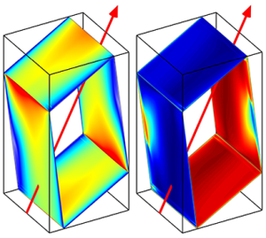
  ${A{\kern-4pt}R} =1/2$, 1 and 2. Both 3-D perspective views and unfolded views of the walls are illustrated (only three walls are shown; the other three walls are the same by symmetry). The
  $x=0.5$ wall, which is parallel to the rotation axis (indicated by a black arrow), shows the footprints of the attractor shear layers depicted in the
  $x=0$ planes in figure 3. On the walls oblique to the rotation axis, footprints of the conical beams emitted from the vertices are evident. On these walls for
  ${A{\kern-4pt}R} =1/2$ and 2,
  $\overline {\boldsymbol {\omega }^2}$ and
  $\boldsymbol {\omega }^2_{SD}$ have strong peaks in the regions where the shear layers in the attractor region reflect at the walls, whereas for
  ${A{\kern-4pt}R} =1$, the peaks are at the tropical edges
  $(y,z)=(\pm 0.5, \pm 0.5{A{\kern-4pt}R} )$ to which beams focus. There is considerable variation in the
  $x$ direction for all cases. Also, away from localised regions where reflections occur,
  $\overline {\boldsymbol {\omega }^2}\sim \sqrt {2}\boldsymbol {\omega }^2_{SD}$, indicating that the oscillatory Ekman layers are nearly harmonic. Supplementary movie 2 animates
  $\boldsymbol {\omega }^2$ on the surface over one libration period
  $\tau ={\rm \pi} /\omega$, and shows that the nearly harmonic oscillations are dominated by progressive waves that sweep through the regions, with more intense
  $\overline {\boldsymbol {\omega }^2}$ corresponding to the shear layer footprints on
  $x=0.5$ and the regions where the shear layers reflect on the
  $y=0.5$ and
  $z=0.5{A{\kern-4pt}R}$ walls.

Figure 8. Scaled  $\overline {\boldsymbol {\omega }^2}$ along the boundary at
  $x=0$, for
  ${A{\kern-4pt}R} =2$ and
  ${E}={Ro}$ as indicated.

Figure 9. Perspective and unfolded views of (a)  $\overline {\boldsymbol {\omega }^2}$ and (b)
  $\sqrt {2}\boldsymbol {\omega }^2_{SD}$ on the cuboid surfaces for
  ${E}={Ro}= 10^{-8}$ and
  ${A{\kern-4pt}R}$ as indicated. Supplementary movie 2 animates
  $\boldsymbol {\omega }^2$ on the surface over a libration period
  $\tau ={\rm \pi} /\omega$.
Now consider the structure of the attractor shear layer. Figure 10 shows  $\overline {\boldsymbol {\omega }^2}$ and
  $\sqrt {2}\boldsymbol {\omega }^2_{SD}$ on two branches of the attractor (the distributions on the other two branches are the same with
  $x\to -x$ by the
  $\mathcal {C}$ symmetry), whose location is predicted from VEBA, for
  ${A{\kern-4pt}R} =2$ and
  ${E}={Ro}\in [10^{-8}, 10^{-5}]$. The general trends on these quantities along the attractor intersection with the meridional plane
  $x=0$ reported in figures 5 and 6 are borne out, but there is considerable variation in the
  $x$ direction, which becomes larger with decreasing
  ${E}$ and
  ${Ro}$. Also evident are signatures of where the conical beams emitted from vertices, and a number of their reflections, intersect the attractor shear layer. For the larger
  ${E}$, these are evident faintly in the mean enstrophy, but as
  ${E}$ is reduced, the amplification of
  $\overline {\boldsymbol {\omega }^2}$ swamps these completely. However, as the enstrophy in the attractor shear layer tends towards a steady state with decreasing
  ${E}$, the conical beam intersections become much more evident in
  $\sqrt {2}\boldsymbol {\omega }^2_{SD}$, as they are locally the dominant contribution to the flow oscillations. The last row in figure 10 shows the intersections with the attractor of the wave beams emitted from edges and vertices, and their subsequent reflections, as determined via VEBA. This captures the fine details in the DNS
  $\sqrt {2}\boldsymbol {\omega }^2_{SD}$ on the attractor, especially for the smaller
  ${E}$ and
  ${Ro}$. This is clear evidence that in the DNS, the wave beams are oscillatory, but as they eventually focus onto the attractor, they fuse into a mean shear flow that locally overwhelms the inertial oscillations.

Figure 10. Illustrations of  $\overline {\boldsymbol {\omega }^2}$ and
  $\sqrt {2}\boldsymbol {\omega }^2_{SD}$ on two branches of the attractor (the other two are the
  $\mathcal {C}$ conjugates), for
  ${A{\kern-4pt}R} =2$ and
  ${E}={Ro}$ as indicated, as well as a 3-D perspective of
  $\overline {\boldsymbol {\omega }^2}$ on the attractor for the case
  ${E}= 10^{-8}$. The bottom row presents intersections with the attractor of the wave beams emitted from edges and vertices, and their subsequent reflections, as determined via VEBA. Supplementary movie 3 includes animations of
  $\boldsymbol {\omega }^2$ over one libration period.
Figures 5, 6, 9 and 10 show that there is a considerable increase in  $\overline {\boldsymbol {\omega }^2}$ as the attractor shear reflects on the walls of the cuboid, and this gain appears to increase as
  ${E}$ and
  ${Ro}$ are reduced. In the linear inviscid regime, VEBA gives what the gains are due solely to geometric focusing at the reflections. For
  ${A{\kern-4pt}R} =2$, the gains
  $g_1$ at reflections on the long walls at
  $y=\pm 0.5$, and
  $g_2$ on the short walls at
  $z=\pm 1$, are (Welfert et al. Reference Welfert, Lopez and Wu2023, (2.5) and (2.7))
 \begin{equation} g_1 = \frac{\sin(\theta+\alpha)}{\sin(\theta-\alpha)} =\frac{{A{\kern-4pt}R}\omega+\sqrt{1-\omega^2}}{{A{\kern-4pt}R}\omega-\sqrt{1-\omega^2}}\approx7.31 \end{equation}
and
 \begin{equation} g_2 = \frac{\cos(\theta+\alpha)}{\cos(\theta-\alpha)} =\frac{\omega+{A{\kern-4pt}R}\sqrt{1-\omega^2}}{\omega-{A{\kern-4pt}R}\sqrt{1-\omega^2}}\approx1.98. \end{equation}
The enstrophy density scales with the fourth power of the gain, and hence increases by approximate factors  $2851$ on the long walls and
  $15.43$ on the short walls. Figure 11 shows how the gains in
  $\overline {\boldsymbol {\omega }^2}$ at these wall reflections vary with decreasing
  ${E}$ and
  ${Ro}$ in the DNS. These gains were determined simply on the
  $x=0$ plane, and clearly figures 9 and 10 show that there is considerable variation in
  $\overline {\boldsymbol {\omega }^2}$ with
  $x$ at the reflections. Nevertheless, the point to be made is that the
  $\overline {\boldsymbol {\omega }^2}$ gains in the DNS with decreasing
  ${E}$ and
  ${Ro}$ surpass the geometric gains from VEBA, indicating that nonlinear processes are playing an increasing role.

Figure 11. Gains in  $\overline {\boldsymbol {\omega }^2}$ at reflections at
  $x=0$ on the long and short walls as functions of
  ${E}$ and
  ${Ro}$ for
  ${A{\kern-4pt}R} =2$.
The primary nonlinear processes contributing to the enhanced gains in  $\overline {\boldsymbol {\omega }^2}$ at the reflections are most likely to be vortex tilting and stretching. These nonlinear mechanisms are inherently 3-D and play a prominent role in hydrodynamics in regimes where the inertial time scale is many orders of magnitude smaller than the viscous time scale, in our case
  ${E}\ll 1$ (Frisch Reference Frisch1996; Majda & Bertozzi Reference Majda and Bertozzi2002; Davidson Reference Davidson2013). Figure 12 shows the magnitudes of the mean and standard deviation of the vortex stretching/tilting term,
  $|\overline {(\boldsymbol {\omega }\boldsymbol {\cdot }\boldsymbol {\nabla })\boldsymbol {v}}|$ and
  $|[(\boldsymbol {\omega }\boldsymbol {\cdot }\boldsymbol {\nabla })\boldsymbol {v}]_{SD}|$, on a long and short attractor branch; supplementary movie 3 includes animations of
  $|{(\boldsymbol {\omega }\boldsymbol {\cdot }\boldsymbol {\nabla })\boldsymbol {v}}|$ over one libration period, and figure 13 shows their profiles at the meridional plane
  $x=0$. As with the enstrophy,
  $|{(\boldsymbol {\omega }\boldsymbol {\cdot }\boldsymbol {\nabla })\boldsymbol {v}}|$ on the attractor tends towards a steady state with decreasing
  ${E}$ and
  ${Ro}$, unsteadiness becoming localised to regions where the attractor reflects on the walls and to a lesser extent where beams emitted from edges and vertices intersect the attractor shear layer. As was the case with
  $\sqrt {2}\boldsymbol {\omega }^2_{SD}$ on the attractor,
  $|[(\boldsymbol {\omega }\boldsymbol {\cdot }\boldsymbol {\nabla })\boldsymbol {v}]_{SD}|$ also matches the VEBA results shown in figure 10.

Figure 12. Illustrations of  $|\overline {(\boldsymbol {\omega }\boldsymbol {\cdot }\boldsymbol {\nabla })\boldsymbol {v}}|$ and
  $|[(\boldsymbol {\omega }\boldsymbol {\cdot }\boldsymbol {\nabla })\boldsymbol {v}]_{SD}|$ on two branches of the attractor (the other two are the
  $\mathcal {C}$ conjugates), for
  ${A{\kern-4pt}R} =2$ and
  ${E}={Ro}$ as indicated. Supplementary movie 3 includes animations of
  $|(\boldsymbol {\omega }\boldsymbol {\cdot }\boldsymbol {\nabla })\boldsymbol {v}|$ over one libration period.

Figure 13. Scaled  $|\overline {(\boldsymbol {\omega }\boldsymbol {\cdot }\boldsymbol {\nabla })\boldsymbol {v}}|$ and
  $|[(\boldsymbol {\omega }\boldsymbol {\cdot }\boldsymbol {\nabla })\boldsymbol {v}]_{SD}|$ as functions of arc length
  $s$ along the attractor (localised using VEBA), for
  ${A{\kern-4pt}R} =2$ and
  ${E}={Ro}$ as indicated.
With nonlinearities not vanishing in the attractor with decreasing  ${E}$ and
  ${Ro}$, it is interesting to determine to what extent
  $\boldsymbol {v}$ and
  $\boldsymbol {\omega }$ are aligned on the attractor, i.e. to determine
  $\alpha =\arccos (\hat {\boldsymbol {\omega }}\boldsymbol {\cdot }\hat {\boldsymbol {v}})$. In the linear inviscid theory of a single circularly polarised inertial wave, either
  $\alpha =0^\circ$,
  $\boldsymbol {\omega }\boldsymbol {\cdot } \boldsymbol {v}>0$ and the group velocity is from south to north, or
  $\alpha =180^\circ$,
  $\boldsymbol {\omega }\boldsymbol {\cdot } \boldsymbol {v}<0$ and the group velocity is from north to south. In open space, such a Beltrami flow has
  $(\boldsymbol {v}\boldsymbol {\cdot }\boldsymbol {\nabla })\boldsymbol {v}=0$. Appendix D shows that there is in general no expectation of alignment between
  $\boldsymbol {v}$ and
  $\boldsymbol {\omega }$ for superpositions of circularly polarised waves, such as on an attractor. Figure 14 shows the mean and standard deviation of
  $\alpha$ along the attractor for
  ${A{\kern-4pt}R} =2$ and various
  ${E}={Ro}$. As
  ${E}$ and
  ${Ro}$ are reduced from
  $10^{-5}$, the flow on the attractor tends to become more Beltrami-like, but as these are reduced below
  $10^{-7}$, this trend is reversed. This departure from Beltrami-like flow for increasingly smaller
  ${E}$ and
  ${Ro}$ is consistent with the flow in the attractor shear layer region becoming increasingly more nonlinear, and the thickness of the shear layers becoming increasingly thinner as they focus onto Delta-like distributions. Figure 15 shows
  $\bar {\alpha }$ and
  $\alpha _{SD}$ on the attractor; the 3-D perspective view for the
  ${E}={Ro}= 10^{-8}$ case illustrates how
  $\bar {\alpha }\approx 180^\circ$ almost everywhere on the branches with the group velocity going north, and
  $\bar {\alpha }\approx 0^\circ$ almost everywhere on the branches with the group velocity going south.

Figure 14. Variations of the mean and standard deviation of  $\alpha =\arccos (\hat {\boldsymbol {v}}\boldsymbol {\cdot }\hat {\boldsymbol {\omega }})$ with arc length
  $s$ along the attractor (localised using VEBA) at
  $x=0$, for
  ${A{\kern-4pt}R} =2$ and
  ${E}={Ro}$ as indicated. Only two branches of the attractor are shown; on the other two branches, the mean angle is
  $180^\circ -\bar {\alpha }$ and the standard deviation is the same.

Figure 15. Mean and standard deviation of the angle between velocity and vorticity,  $\alpha =\arccos (\hat {\boldsymbol {\omega }}\boldsymbol {\cdot }\hat {\boldsymbol {v}})$, on two branches of the attractor, for
  ${A{\kern-4pt}R} =2$ and
  ${E}={Ro}$ as indicated, as well as a 3-D perspective of
  $\bar {\alpha }$ on the attractor for the case
  ${E}= 10^{-8}$. Supplementary movie 3 includes animations of
  $\alpha$ over one libration period.
5. Zeroth law:  ${E}\mathcal {E}\ne 0$ as ${E}\to 0$


In this section, the global energy balance is considered for decreasing  ${E}$ and
  ${Ro}$. Using
  $\boldsymbol {\nabla } \boldsymbol {\cdot } \boldsymbol {v}=0$ and the identities
 \begin{equation} (\boldsymbol{v}\boldsymbol{\cdot}{\boldsymbol{\nabla}})\boldsymbol{v}= {\boldsymbol{\nabla}}\left(\frac{\boldsymbol{v}^2}{2}\right)+ \boldsymbol{\omega}\times\boldsymbol{v} \quad \textrm{and}\quad {\nabla}^2\boldsymbol{v}= {\boldsymbol{\nabla}}({\boldsymbol{\nabla}}\boldsymbol{\cdot}\boldsymbol{v})-{\boldsymbol{\nabla}}\times\boldsymbol{\omega}={-}{\boldsymbol{\nabla}}\times\boldsymbol{\omega}, \end{equation}
the Navier–Stokes equation (2.3) can be rewritten as
 \begin{equation} \frac{\partial \boldsymbol{v}}{\partial t} +{\boldsymbol{\nabla}}\left(p_r+{Ro}\,\frac{\boldsymbol{v}^2}{2}\right) +({Ro}\,\boldsymbol{\omega}+2\boldsymbol{\varOmega}) \times \boldsymbol{v} +{E}\,{\boldsymbol{\nabla}}\times\boldsymbol{\omega} = 2\omega\sin(2\omega t)\,\boldsymbol{\varOmega}_0\times\boldsymbol{x}. \end{equation}
Multiplying (5.2) by  $\boldsymbol {v}$, using
  $\boldsymbol {\nabla }\boldsymbol {\cdot } \boldsymbol {v}=0$ and the identity
 \begin{equation} \boldsymbol{v}\boldsymbol{\cdot}({\boldsymbol{\nabla}}\times\boldsymbol{\omega})= \boldsymbol{\omega}^2+{\boldsymbol{\nabla}}\boldsymbol{\cdot}(\boldsymbol{\omega}\times\boldsymbol{v}), \end{equation}
yields the energy equation (Wu et al. Reference Wu, Welfert and Lopez2022b)
 \begin{align} \frac{\partial}{\partial t}\left(\frac{\boldsymbol{v}^2}{2}\right) +{E} \boldsymbol{\omega}^2 - 2\omega\sin(2\omega t)\, \boldsymbol{v}\boldsymbol{\cdot}(\boldsymbol{\varOmega}_0\times\boldsymbol{x}) ={-}{\boldsymbol{\nabla}}\boldsymbol{\cdot}\left[ \left(p_r +{Ro}\,\frac{\boldsymbol{v}^2}{2}\right)\boldsymbol{v} +E (\boldsymbol{\omega}\times\boldsymbol{v})\right]. \end{align}
Integrating (5.4) over the volume of the cuboid  $\mathcal {V}$ leads to
 \begin{equation} {{\rm d} \mathcal{K}}/{{\rm d} t} + {E}\mathcal{E} + \mathcal{W} = \mathcal{D}(\boldsymbol{v}), \end{equation}
where
 \begin{equation} \mathcal{K} =\int_{\mathcal{V}} \frac{\boldsymbol{v}^2}{2}\,{\rm d}\boldsymbol{x} \end{equation}
is the kinetic energy,
 \begin{equation} \mathcal{E} =\int_{\mathcal{V}} \boldsymbol{\omega}^2 \, {\rm d} \boldsymbol{x} \end{equation}
is the enstrophy,
 \begin{equation} \mathcal{W}={-}2\omega\sin(2\omega t) \int_{\mathcal{V}}\boldsymbol{v}\boldsymbol{\cdot}(\boldsymbol{\varOmega}_0 \times\boldsymbol{x})\,{\rm d} \boldsymbol{x} \end{equation}
is the work done by the librational (Euler) force, with  $\boldsymbol {v}\boldsymbol {\cdot }(\boldsymbol {\varOmega }_0\times \boldsymbol {x})= \boldsymbol {\varOmega }_0\boldsymbol {\cdot }(\boldsymbol {x}\times \boldsymbol {v})$ the (relative) axial angular momentum, and
 \begin{equation} \mathcal{D}(\boldsymbol{v})={-}\int_{\mathcal{V}}{\boldsymbol{\nabla}}\boldsymbol{\cdot}\left[ \left(p_r +{Ro}\,\frac{\boldsymbol{v}^2}{2}\right)\boldsymbol{v} +E (\boldsymbol{\omega}\times\boldsymbol{v})\right]\, {\rm d} \boldsymbol{x} \end{equation}
is a residual term. When  $\boldsymbol {v}$ has sufficient regularity, Gauss's divergence theorem together with the no-slip boundary conditions results in
  $\mathcal {D}(\boldsymbol {v})=0$. This is the case for numerical simulations with sufficient spatial resolution obtained at small but non-zero
  ${E}$.
Figure 16 plots the three terms on the left-hand side of (5.5) over one libration period  $\tau ={\rm \pi} /\omega$ for
  ${A{\kern-4pt}R} =2$ and
  ${E}={Ro}\in [10^{-8}, 10^{-5}]$, with
  ${\rm d} \mathcal {K}/ {\rm d} t$ determined from the time series of
  $\mathcal {K}$ via Fourier spectral differentiation. The figure shows that
  ${{\rm d} \mathcal {K}}/{{\rm d} t}$ and
  $\mathcal {W}$ almost balance each other. The dissipation term
  ${E}\mathcal {E}$ is much smaller but appears to remain bounded away from zero with decreasing
  ${E}$. This property is known as the zeroth law or the dissipative anomaly in the context of turbulent flows (Onsager Reference Onsager1949; Dubrulle Reference Dubrulle2019; Drivas Reference Drivas2022). The same property holds here as a result of large gradients that develop in the direction transverse to the increasingly thinner interior viscous shear layers that ultimately lead to the low-regularity properties of the attractor as
  ${E}\to 0$. The finite size of
  ${E}\mathcal {E}$ is consistent with the scaling
  $\overline {\boldsymbol {\omega }^2}\sim {E}^{-4/3}$ obtained in figure 5 along the interior viscous shear layer, over a shear layer thickness of order
  ${E}^{1/3}$ at small non-zero
  ${E}$. Note that in the regions where the beams forming the shear layer reflect on the walls, they are more intense, with a scaling
  $\overline {\boldsymbol {\omega }^2}\sim {E}^{-5/3}$ (see figure 6). This occurs in localised regions with an extent scaling with
  ${E}^{(1/2+1/2)}$, corresponding to the combination of viscous boundary layer depth (
 ${E}^{1/2}$) and the along-wall region of the reflections (
 ${E}^{1/2}$), resulting in a vanishing contribution to
  ${E}\mathcal {E}$ as
  ${E}\to 0$.

Figure 16. Variations over one libration period of the three terms on the left-hand side of (5.5),  ${{\rm d} \mathcal {K}}/{{\rm d} t}$,
  ${E}\mathcal {E}$ and
  $\mathcal {W}(\boldsymbol {v})$, and their sum, for
  ${A{\kern-4pt}R} =2$ and
  ${E}={Ro}$ as indicated.
The sum of the terms on the left-hand side of (5.5), shown in figure 16, although at least four orders of magnitude smaller than both  ${\rm d} \mathcal {K}/ {\rm d} t$ and
  $\mathcal {W}$, and an order of magnitude smaller than the mean dissipation
  ${E}\mathcal {E}$, does not seem to vanish as
  ${E}\to 0$. In this limit, (5.5) has to be understood in a distributional sense, and
  $\mathcal {D}(\boldsymbol {v})$ may not vanish, resulting in anomalous dissipation.
Figure 17 plots the three terms on the left-hand side of (5.5) and their sum for the  ${E}= 10^{-8}$ case computed with a range of spatial resolution (using Legendre polynomials of degree ranging from
  $M=500$ to
  $M=650$). The results are virtually indistinguishable, indicating that the numerical solutions are well converged, and the finite dissipation and anomaly observed in figure 16 are not numerical artefacts.

Figure 17. Variations over one libration period of the three terms on the left-hand side of (5.5),  ${{\rm d} \mathcal {K}}/{{\rm d} t}$,
  ${E}\mathcal {E}$ and
  $\mathcal {W}(\boldsymbol {v})$, and their sum, for
  ${A{\kern-4pt}R} =2$ and
  ${E}={Ro}= 10^{-8}$, and spatial resolution
  $M$ as indicated.
6. Summary and conclusions
A detailed numerical investigation of the structure of inertial wave attractors in rectilinear cuboids is conducted at very small Ekman and Rossby numbers in order to assess which aspects are captured by the linear inviscid theory, implemented in the vertex and edge beam analysis (VEBA) presented in Welfert et al. (Reference Welfert, Lopez and Wu2023), and which are not. VEBA captures most of the geometric features of the intricate network of shear layers emanating from edges and vertices, and their ultimate focusing, at the forcing frequency considered, onto an attractor. This attractor has a quasi-invariant structure in the  $x$ direction as a result of the container walls at
  $x=\pm 0.5$ being parallel to the rotation axis. VEBA also predicts correctly the blow-up of enstrophy density at the attractor due to the overall geometric focusing of wave beams at wall reflections.
The simulations of the full incompressible Navier–Stokes system enable a quantification of this blow-up as the Ekman and Rossby numbers are decreased, with a resulting global viscous dissipation that does not vanish, but instead approaches a static, positive mean value. The development of a non-trivial mean flow in attractor shear layers has also been reported in forced rotating spherical shells (Tilgner Reference Tilgner2007). Our simulations also show that vortex stretching and tilting persist within the attractor, as well as where beams of energy interact with each other, with decreasing Ekman and Rossby numbers, so that the flows are fundamentally three-dimensional and nonlinear. Even for extremely small forcing amplitudes, nonlinear effects have important dynamic consequences for the shear layers forming on attractors. Such a dichotomy between predictions of attractors based on linear inviscid theory and their intrinsically nonlinear and dissipative nature has long been recognised (Maas Reference Maas2005). The configuration studied here, in which the flow remains a perfectly symmetric synchronous limit cycle, not only offers a simple set-up for studying the roles of dissipative and nonlinear effects on inertial waves, but is also a promising candidate for assessing numerically the existence of anomalous dissipation and/or work in the limits of vanishing Ekman and Rossby numbers.
Supplementary movies
Supplementary movies are available at https://doi.org/10.1017/jfm.2023.772.
Acknowledgements
The authors thank ASU Research Computing for use of their facilities.
Declaration of interests
The authors report no conflict of interest.
Appendix A. Relationship between flows in $1\times 1\times a$ and $1/a\times 1\times 1/a$ cuboids


The solution  $\boldsymbol {v}$ and
  $p_r$ to (2.3), in a
  $1\times 1\times a$ cuboid rotating around an axis directed by
  $\boldsymbol {\varOmega }_0=(0,1,a)/\sqrt {1+a^2}$, is related to the solution
  $\tilde {\boldsymbol {v}}$ and
  $\widetilde {p_r}$ in a
  $1/a\times 1\times 1/a$ cuboid rotating around
  $\widetilde {\boldsymbol {\varOmega }_0}=(0,a,1)/\sqrt {1+a^2}$, described by a modified version of (2.3) derived below, using the same length scale
  $L$; see figure 18.

Figure 18. Relationship between flows in  $1\times 1\times a$ and
  $1/a\times 1\times 1/a$ cuboids.
Let
 \begin{equation} \boldsymbol{x}={\boldsymbol{\mathsf{S}}}\tilde{\boldsymbol{x}}, \quad \boldsymbol{v}(\boldsymbol{x},t)={\boldsymbol{\mathsf{S}}}\,\tilde{\boldsymbol{v}} (\tilde{\boldsymbol{x}},t) \quad\text{and}\quad p_r(\boldsymbol{x},t)=a^2\,\widetilde{p_r}(\tilde{\boldsymbol{x}},t), \end{equation}
with
 \begin{equation} {\boldsymbol{\mathsf{R}}}=\begin{bmatrix} -1 & 0 & 0\\\phantom{-}0 & 0 & 1\\\phantom{-}0 & 1 & 0\end{bmatrix} \quad\text{and}\quad {\boldsymbol{\mathsf{S}}}=a{\boldsymbol{\mathsf{R}}}. \end{equation}
Here,  ${\boldsymbol{\mathsf{S}}}$ maps each point
  $\tilde {\boldsymbol x}\in [-0.5/a,0.5/a]\times [-0.5,0.5]\times [-0.5/a,0.5/a]$ to a point
  $\boldsymbol {x}\in [-0.5,0.5]^2\times [-0.5a,0.5a]$, and
  ${\boldsymbol{\mathsf{R}}}$ is the matrix of a rotation of angle
  ${\rm \pi}$ around the axis directed by
  $(0,1,1)$.
The following relations all hold:
 \begin{equation} \left.\begin{array}{c} \partial\boldsymbol{v}/\partial t = {\boldsymbol{\mathsf{S}}}\,\partial\tilde{\boldsymbol{v}}/\partial t, \\[2pt] (\boldsymbol{v}\boldsymbol{\cdot}{\boldsymbol{\nabla}})\boldsymbol{v}= {\boldsymbol{\mathsf{S}}}[(\tilde{\boldsymbol{v}}\boldsymbol{\cdot}\tilde{\boldsymbol{\nabla}}) \tilde{\boldsymbol{v}}], \\[2pt] \boldsymbol{\varOmega}_0= {\boldsymbol{\mathsf{R}}}\widetilde{\boldsymbol{\varOmega}_0}, \\[2pt] \boldsymbol{\varOmega}_0\times\boldsymbol{x}= {\boldsymbol{\mathsf{S}}}\widetilde{\boldsymbol{\varOmega}_0} \times{\boldsymbol{\mathsf{R}}}\tilde{\boldsymbol{x}} ={\boldsymbol{\mathsf{S}}}[\widetilde{\boldsymbol{\varOmega}_0} \times\tilde{\boldsymbol{x}}], \\[2pt] \boldsymbol{\varOmega}_0\times\boldsymbol{v}= {\boldsymbol{\mathsf{S}}}\widetilde{\boldsymbol{\varOmega}_0} \times{\boldsymbol{\mathsf{R}}}\tilde{\boldsymbol{v}} ={\boldsymbol{\mathsf{S}}}[\widetilde{\boldsymbol{\varOmega}_0} \times\tilde{\boldsymbol{v}}], \\[2pt] {\boldsymbol{\nabla}}p_r = a^2{\boldsymbol{\mathsf{S}}}^{{-}1}\,\tilde{\boldsymbol{\nabla}}\widetilde{p_r} ={\boldsymbol{\mathsf{S}}}\,\tilde{\boldsymbol{\nabla}}\widetilde{p_r}, \\[2pt] {\nabla}^2\boldsymbol{v}= a^{{-}1}{\boldsymbol{\mathsf{R}}}\, \tilde{\nabla}^2\tilde{\boldsymbol{v}} =a^{{-}2}{\boldsymbol{\mathsf{S}}}\,\tilde{\nabla}^2\tilde{\boldsymbol{v}}, \end{array}\right\} \end{equation}
where  $\tilde {\boldsymbol {\nabla }} = {\boldsymbol {\nabla }}_{\tilde {\boldsymbol {x}}}$.
As a result, (2.2) becomes
 \begin{equation} \frac{\partial \tilde{\boldsymbol{v}}}{\partial t} +{Ro}\,(\tilde{\boldsymbol{v}}\boldsymbol{\cdot}\tilde{\boldsymbol{\nabla}})\tilde{\boldsymbol{v}} +2\tilde{\boldsymbol{\varOmega}} \times \tilde{\boldsymbol{v}} + \frac{{\rm d} \tilde{\boldsymbol{\varOmega}}}{{\rm d} t} \times \tilde{\boldsymbol{x}} ={-}\tilde{\boldsymbol{\nabla}}\widetilde{p_r} +\tilde{{E}}\,\tilde{\nabla}^2\tilde{\boldsymbol{v}}, \quad \tilde{\boldsymbol{\nabla}}\boldsymbol{\cdot}\tilde{\boldsymbol{v}}=0, \end{equation}
with  $\tilde {\boldsymbol {\varOmega }}=[1+{Ro} \cos (2\omega t)] \widetilde {\boldsymbol {\varOmega }_0}$ and
  $\tilde {{E}} = {E}/a^2$. Since
  ${\boldsymbol {\nabla }}\times \boldsymbol {v}= {\boldsymbol{\mathsf{R}}}\,\tilde {\boldsymbol {\nabla }}\times \tilde {\boldsymbol {v}}$,
  $\boldsymbol {v}$ and
  $\tilde {\boldsymbol {v}}$ have equal enstrophy density at corresponding locations
  $\boldsymbol {x}$ and
  $\tilde {\boldsymbol {x}}$. If the immersed length of the rotation axis,
  $\tilde {L}=L\sqrt {1+a^2}$, had been used as the length scale instead of
  $L$, then
 \begin{equation} \tilde{{E}}(1/a)=a^{{-}2}\,{E}(1/a)=a^{{-}2}\nu/[\varOmega \tilde{L}^2(1/a)] =\nu/[\varOmega\tilde{L}^2(a)]={E}(a). \end{equation}
Appendix B. Traces in $x=0$ of conical vertex beams and edge beams from edges in the $y$ direction


Potentially, each vertex of the cuboid emits wave beams into the cuboid along rays on a cone of aperture  $2\vartheta$ with its apex at that vertex and its axis directed by
  $\boldsymbol {\varOmega }_0$. For
  $\omega =0.55$ considered here,
  $\vartheta =\arcsin \omega \approx 33.4^\circ$. The cone with apex at
  $\boldsymbol {\nu }=(X,Y,Z)=(0,0,0)$, where
  $(X,Y,Z)=(x-0.5,y-0.5,z-0.5{A{\kern-4pt}R} )$, is illustrated in figure 19. It is parametrised by (Wu et al. Reference Wu, Welfert and Lopez2022b, (4.5))
 \begin{align} \boldsymbol{\nu}+t\hat{\boldsymbol{a}}_+ &= t[\cos\vartheta\,\boldsymbol{\varOmega}_0+ \sin\vartheta\,(\cos\varphi\,\widehat{\boldsymbol{e}_x}+ \sin\varphi\,\boldsymbol{\varOmega}_0\times\widehat{\boldsymbol{e}_x})] \nonumber\\ &=\frac{t}{\sqrt{{A{\kern-4pt}R}^2+1}} \begin{bmatrix} \sqrt{{A{\kern-4pt}R}^2+1} \sin\vartheta\cos\varphi\\ \cos\vartheta+{A{\kern-4pt}R}\sin\vartheta\sin\varphi\\ {A{\kern-4pt}R}\cos\vartheta-\sin\vartheta\sin\varphi \end{bmatrix}, \end{align}
and intersects the plane  $X=0.5$ (
 $x=0$) along the hyperbolic conic section
 \begin{equation} (Y,Z) = 0.5(\cot\vartheta\sec\varphi+{A{\kern-4pt}R}\tan\varphi, {A{\kern-4pt}R}\cot\vartheta\sec\varphi-\tan\varphi)/ \sqrt{{A{\kern-4pt}R}^2+1}, \end{equation}
shown in red in figure 19. The limits
 \begin{equation} \varphi\in[-\arcsin(\cot\vartheta/{A{\kern-4pt}R}),\alpha- \arcsin(\cot\vartheta/\sqrt{5{A{\kern-4pt}R}^2+4})], \end{equation}
with  $\tan \alpha =2\sqrt {{A{\kern-4pt}R} ^2+1}/{A{\kern-4pt}R}$, guarantee
  $Y\in [0,1]$. Edge beams are emitted from points at
  $X=Z=0$ in a direction such that the resulting planar edge sheet is tangent to the conic sheet from
  $\boldsymbol {\nu }$. This direction is that of the line between
  $\boldsymbol {\nu }$ and the point in the plane
  $x=0$ corresponding to the minimum of
  $Z$ in (B2):
 \begin{equation} Z'(\varphi)=0\Rightarrow {A{\kern-4pt}R}\cot\vartheta\sec\varphi\tan\varphi =\sec^2\varphi \Rightarrow \sin\varphi=\tan\vartheta/{A{\kern-4pt}R}. \end{equation}
We have  $\tan \vartheta /{A{\kern-4pt}R} <1$ only for
  ${A{\kern-4pt}R} >1$ when interior attractors exist (Welfert et al. Reference Welfert, Lopez and Wu2023). Substitution into (B2) then yields the coordinates
 \begin{equation} (Y,Z) = \left(\frac{1}{2\omega\sqrt{{A{\kern-4pt}R}^2+1} \sqrt{1-\omega^2(1+{A{\kern-4pt}R}^{{-}2})}}, \frac{{A{\kern-4pt}R}\sqrt{1-\omega^2(1+{A{\kern-4pt}R}^{{-}2})}}{2\omega\sqrt{{A{\kern-4pt}R}^2+1}}\right) \end{equation}
of the point in the conic section with minimum  $Z$ (i.e.
  $z$). This point always has
  $Z<{A{\kern-4pt}R} /2$, i.e.
  $z<0$, but has
  $Y<1$ only for
 \begin{equation} \left|\omega^2-\frac{1}{2(1+{A{\kern-4pt}R}^{{-}2})}\right|< \frac{\sqrt{1-{A{\kern-4pt}R}^{{-}2}}}{2(1+{A{\kern-4pt}R}^{{-}2})}. \end{equation}
Figure 19. Conic vertex sheet emitted from the vertex at  $(x,y,z)=(-0.5,-0.5,-0.5{A{\kern-4pt}R} )$ and planar edge sheet emitted from the edge
  $(x,z)=(-0.5,-0.5{A{\kern-4pt}R} )$ (both shown in grey), together with their traces (thick red curve) in the meridional plane
  $x=0$ (cyan), for a cuboid with
  ${A{\kern-4pt}R} =2$ and
  $\omega =0.55$. Only the portion of the edge sheet with
  $x<0$ is shown. The red dashed line represents the intersection of a similar conic sheet emitted from the apex at
  $(x,y,z)=(-0.5,0.5,-0.5{A{\kern-4pt}R} )$.
For  ${A{\kern-4pt}R} =2$ and
  $\omega =0.55$ considered here, (B6) reduces to
  $|0.3025-0.4|<\sqrt {3}/5\approx 0.35$, which is satisfied. The trace of the resulting edge sheet emanating from the edge at
  $X=Z=0$ is then a line segment from
  $(0.5,Y,Z)$ to
  $(0.5,1,Z)$ with
  $(Y,Z)$ given by (B2), also shown in red in figure 19. Note that (B6) extends to the whole inertial range as
  ${A{\kern-4pt}R} \to \infty$, in which case
  $Y<1$ is typical and the manifestation of the edge sheet is visible in the meridional plane
  $x=0$. On the other hand, (B6) does not intersect the attractor region
  $\omega ^2\in ({A{\kern-4pt}R} ^{-2}/[1+{A{\kern-4pt}R} ^{-2}],1/[1+{A{\kern-4pt}R} ^{-2}])$ if
  ${A{\kern-4pt}R} <2/\sqrt {3}$, and the edge sheet cannot be observed in the plane
  $x=0$.
The vertex at  $(X,Y,Z)=(0,1,{A{\kern-4pt}R} )$, i.e.
  $(x,y,z)=(-0.5,0.5,0.5{A{\kern-4pt}R} )$, emits conic beams whose intersections with
  $x=0$ are symmetric about
  $(x,y,z)=(0,0,0)$ compared with those emitted from
  $\boldsymbol {\nu }$. Likewise, the edge
  $(x,y,z)=(-0.5,y,0.5{A{\kern-4pt}R} )$ emits a planar edge sheet with a trace that is the symmetric image of the one from
  $(x,y,z)=(-0.5,y,-0.5{A{\kern-4pt}R} )$. Vertices and edges at
  $x=+0.5$ emit beams that are mirror images, with respect to
  $x=0$, of those emitted from
  $x=-0.5$, and thus have the same trace in the plane
  $x=0$. No wave beam seems to be emitted from the vertices
  $(x,y,z)=(\pm 0.5,0.5,-0.5{A{\kern-4pt}R} )$ and
 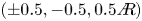 $(\pm 0.5,-0.5,0.5{A{\kern-4pt}R} )$, despite the respective cones having a non-trivial intersection with the cuboid. Their would-be traces in the plane
  $x=0$, one of which is represented by a dashed line in figure 19, are absent in the DNS. This resolves an outstanding question raised in Welfert et al. (Reference Welfert, Lopez and Wu2023) about conflicting tangentiality requirements between (planar) edge sheets and (conic) vertex sheets emanating from the endpoints of the edge: one vertex sheet dictates the orientation of the edge sheet, which in turn prevents the other vertex from emitting if it cannot merge tangentially.
Appendix C. Relation between mean and standard deviation of the square of a periodic function
Consider a periodic function  $f:\mathbb {R}\to \mathbb {R}$ with period
  $\tau ={\rm \pi} /\omega$ and Fourier expansion
 \begin{equation} f(t) = \sum_{k\in\mathbb{Z}} a_k\, {\rm e}^{2 {\rm i}k\omega t}, \end{equation}
with  $a_k$ and
  $a_{-k}$ conjugate. Then
 \begin{equation} [f(t)]^2 = \sum_{k,\ell\in\mathbb{Z}} a_ka_\ell \, {\rm e}^{2 {\rm i}(k+\ell)\omega t} \Rightarrow \overline{[f(t)]^2} =\sum_{k\in\mathbb{Z}}a_ka_{{-}k} =\sum_{k\in\mathbb{Z}}|a_k|^2 \end{equation}
and
 \begin{equation} [f(t)]^4 = \sum_{k,\ell,m,n\in\mathbb{Z}} a_ka_\ell a_ma_n \, {\rm e}^{2 {\rm i}(k+\ell+m+n)\omega t} \Rightarrow \overline{[f(t)]^4}= \sum_{k,\ell,m,n\in\mathbb{Z} \atop k+\ell+m+n=0} a_ka_\ell a_ma_n, \end{equation}
where the over-bar designates taking the time average over the period  $\tau$. The ratio of the variance of
  $f^2$ to the square of its mean is the factor
 \begin{equation} \gamma:=\frac{\overline{([f(t)]^2- \overline{[f(t)]^2})^{2}} }{\overline{[f(t)]^2}^2}= \frac{\overline{[f(t)]^4}}{\overline{[f(t)]^2}^2}-1= \frac{\displaystyle \sum_{k,\ell,m,n\in\mathbb{Z} \atop k+\ell+m+n=0}a_ka_\ell a_ma_n}{\left(\displaystyle \sum_{k\in\mathbb{Z}}|a_k|^2\right)^2}-1. \end{equation}
 For a purely harmonic function with  $a_0=a_{\pm 2}=a_{\pm 3}=\cdots =0$,
  $\{k,\ell,m,n\}=\{1,1,-1,-1\}$. Since there are
  ${4\choose 2}=6$ such arrangements, the ratio (C4) becomes
 \begin{equation} \gamma_1=\frac{6a_1^2a_{{-}1}^2}{(|a_1|^2+|a_{{-}1}|^2)^2}-1 =\frac{6|a_1|^4}{4|a_1|^4}-1=\frac{1}{2}. \end{equation}
Thus the ratio of the standard deviation to the mean of  $f^2$, with
  $f$ harmonic, is
  $\sqrt {\gamma _1}=1/\sqrt {2}$.
For a function  $f$ with
  $a_k=0$ for
  $|k|>2$, there are eight possible combinations of four values from
  $\{0,\pm 1,\pm 2\}$ with
  $0$ sum, summarised in table 2. As a result,
 \begin{align} &\gamma_2+1 \nonumber\\ &\quad =\frac{a_0^4+6(a_1^2a_{{-}1}^2+a_2^2a_{{-}2}^2) +12(a_0^2a_1a_{{-}1}+a_0^2a_2a_{{-}2}+a_0a_1^2a_{{-}2} +a_0a_{{-}1}^2a_2)+ 24a_1a_2a_{{-}1}a_{{-}2}}{(a_0^2 +|a_1|^2+|a_{{-}1}|^2+|a_2|^2+|a_{{-}2}|^2)^2} \nonumber\\ &\quad =\frac{a_0^4+6(|a_1|^4+|a_2|^4) +12(a_0^2|a_1|^2+a_0^2|a_2|^2+2\,{\rm Re}[a_0a_1^2a_{{-}2}]) +24|a_1|^2|a_2|^2}{(a_0^2+2|a_1|^2+2|a_2|^2)^2}. \end{align}
Table 2. Number of arrangements of zero-sum quadruplets  $\{k,\ell,m,n\}$ from values in
  $\{0,\pm 1,\pm 2\}$.

If  $f$ is weakly non-harmonic, i.e.
  $|a_0|,|a_2|\approx \varepsilon |a_1|$ with
  $\varepsilon \ll 1$, then
 \begin{equation} \gamma_2\approx \frac{6+12(1+2\cos\varphi)\varepsilon^2+24\varepsilon^2} {(2+3\varepsilon^2)^2}-1 \approx\frac{1}{2}(1+(12\cos\varphi-3)\varepsilon^2), \end{equation}
where  $\varphi$ represents the phase of
  $a_1^2a_{-2}$. The ratio of the standard deviation to the mean of
  $f^2$ thus becomes
  $\sqrt {\gamma _2}\approx [1+(6\cos \varphi -1.5)\varepsilon ^2]/\sqrt {2}$.
The ratio (C6) can be shown to reach its maximum, approximately  $3.48$, for
  $|a_0|\approx 0.93\,|a_1|$ and
  $|a_2|\approx 0.74\,|a_1|$. Thus
  $\sqrt {\gamma _2}\lesssim 2.64/\sqrt {2}$. Larger values of (C4) can be obtained for sequences
  $\{|a_k|\}_{k \ge 0}$ decreasing only slowly (e.g. algebraically) with
  $k$, as a result of the dimensionality of the summations involved (
 $4-1=3$ for the numerator versus
  $2\times 1=2$ for the denominator). This slow decrease is associated typically with low regularity of
  $f$, that may, for example, result from spatial low regularity for
  $f^2=\boldsymbol {\omega }^2$ associated with the solution of (2.3).
Appendix D. Non-alignment of velocity and vorticity in attractor region
The inviscid theory predicts correctly the location of the attractor by considering circularly polarised waves (Wu, Welfert & Lopez Reference Wu, Welfert and Lopez2020b), with
 \begin{equation} \boldsymbol{v} \approx \boldsymbol{a}\sin\varphi+\boldsymbol{b}\cos\varphi, \quad \varphi = \boldsymbol{k}\boldsymbol{\cdot}\boldsymbol{x}-2\omega t, \quad \boldsymbol{b}={\pm}\boldsymbol{a}\times\hat{\boldsymbol{k}}. \end{equation}
The orthogonality between the direction  $\boldsymbol {a}$ of energy propagation and the wavevector
  $\boldsymbol {k}$, i.e.
  $\boldsymbol {a}\boldsymbol {\cdot }\boldsymbol {k}=0$, implies that the nonlinear term
  $(\boldsymbol {v}\boldsymbol {\cdot }{\boldsymbol {\nabla }})\boldsymbol {v}$ or equivalently, the Lamb vector
  $\boldsymbol {\omega }\times \boldsymbol {v}$, vanishes. Specifically, (D1) yields
  $\boldsymbol {\omega }={\boldsymbol {\nabla }}\times \boldsymbol {v}=\mp |\boldsymbol {k}|\,\boldsymbol {v}$. In general, however, superpositions of circularly polarised waves
  $\boldsymbol {v}_1$ and
  $\boldsymbol {v}_2$ of the form (D1) are themselves not circularly polarised. Indeed,
 \begin{align} \pm{\boldsymbol{\nabla}}\times(\boldsymbol{v}_1+\boldsymbol{v}_2)\times(\boldsymbol{v}_1+\boldsymbol{v}_2) =(|\boldsymbol{k}_1|\,\boldsymbol{v}_1+|\boldsymbol{k}_2|\,\boldsymbol{v}_2)\times(\boldsymbol{v}_1+\boldsymbol{v}_2) =(|\boldsymbol{k}_1|-|\boldsymbol{k}_2|) \boldsymbol{v}_1\times\boldsymbol{v}_2 \end{align}
shows that  $\boldsymbol {v}_1+\boldsymbol {v}_2$ aligns with its curl only if the waves have the same wavelength,
  $|\boldsymbol {k}_1|=|\boldsymbol {k}_2|$, or if their velocity vectors
  $\boldsymbol {v}_1$ and
  $\boldsymbol {v}_2$ are aligned at all times. A beam
  $\boldsymbol {a}_1$ tracing exactly on the attractor onto a beam
  $\boldsymbol {a}_2$ will have
  $|\boldsymbol {k}_2|>|\boldsymbol {k}_1|$ due to focusing at wall reflections, while the phases
  $\varphi _1$ and
  $\varphi _2$ will in general be different, depending on the length of the attractor. As such, no alignment of the vorticity with the velocity can be expected at the attractor.


 Open access