


1. Introduction
As random gravity waves pass over abrupt depth decreases, there is a locally increased probability of the occurrence of extreme waves. This was identified by Trulsen, Zeng & Gramstad (Reference Trulsen, Zeng and Gramstad2012) and has since motivated many researchers to investigate this using numerical, analytical and experimental methods (Gramstad et al. Reference Gramstad, Zeng, Trulsen and Pedersen2013; Bolles, Speer & Moore Reference Bolles, Speer and Moore2019; Majda, Moore & Qi Reference Majda, Moore and Qi2019; Zhang et al. Reference Zhang, Benoit, Kimmoun, Chabchoub and Hsu2019; Monsalve et al. Reference Monsalve, Maurel, Pagneux and Petitjeans2022) (see also figure 1 in Li et al. (Reference Li, Draycott, Adcock and van den Bremer2021a)). Two main mechanisms have been suggested to explain this phenomenon. One is that, as the waves pass over the depth discontinuity, they go out of equilibrium and, as they adjust, correlations occur between constituents, leading to an increased number of large waves (Viotti & Dias Reference Viotti and Dias2014; Mendes et al. Reference Mendes, Scotti, Brunetti and Kasparian2022). Waves adjusting to a new equilibrium can certainly provoke rogue waves (Waseda, Toba & Tulin Reference Waseda, Toba and Tulin2001; Annenkov & Shrira Reference Annenkov and Shrira2006; Trulsen Reference Trulsen2018; Tang et al. Reference Tang, Barratt, Bingham, van den Bremer and Adcock2022). However, there is stronger direct evidence for a second mechanism suggested for the increase in rogue waves at the top of steps. This is that, as the waves pass over the depth discontinuity, the bound wave structure has to change, leading to the release of freely propagating components, the most significant of which are at double the frequency of the dominant waves. This free wave travels at a different speed to the dominant wave, leading to correlations in phase some distance from the depth discontinuity. This theory was developed by Massel (Reference Massel1983), Monsalve Gutiérrez (Reference Monsalve Gutiérrez2017) and Li et al. (Reference Li, Zheng, Lin, Adcock and van den Bremer2021c) and extended by Li et al. (Reference Li, Draycott, Zheng, Lin, Adcock and van den Bremer2021b) to a statistical model whose predictions show good agreement with numerics and experiments.
A key limitation of the work to date is that only unidirectional waves have been considered, unlike waves in the real ocean, which are directionally spread. The exception to this is the work of Ducrozet & Gouin (Reference Ducrozet and Gouin2017), who used a higher-order spectral scheme to model both unidirectional waves and waves with  $11^{\circ }$ directional spreading passing over the bathymetry considered in Trulsen et al. (Reference Trulsen, Zeng and Gramstad2012). They found that an excess number of rogue waves still occurred for the directionally spread case. A number of studies have started with unidirectional waves and analysed the propagation over three-dimensional geometries (Trulsen et al. Reference Trulsen, Raustøl, Jorde and Bæverfjord Rye2020; Lawrence, Trulsen & Gramstad Reference Lawrence, Trulsen and Gramstad2021) and Zeng & Trulsen (Reference Zeng and Trulsen2012) have used a variable-depth version of the nonlinear Schrödinger equation to study waves moving over less abrupt slopes in deeper water, where the results are expected to be different. Their results have also been successfully recreated in a recent study by Lawrence, Trulsen & Gramstad (Reference Lawrence, Trulsen and Gramstad2022) with a fully nonlinear implementation of the Euler equations. Lyu, Mori & Kashima (Reference Lyu, Mori and Kashima2023) have also studied directional waves moving over shallower slopes, which are expected to behave differently to abrupt depth transitions. Theoretical work on the travel direction in which any released bound waves will propagate has been given in Li, Liang & Draycott (Reference Li, Liang and Draycott2022a), which, along with an alternative theoretical model, is compared to numerical results in Li (Reference Li2022). Understanding this is an important first step to building a statistical model for rogue wave occurrence in directional seas. In the present paper, we explore how varying directional spreading influences the probability of a rogue wave occurring at the top of a slope using experiments and fully nonlinear numerical simulations.
2. Method
2.1. Experiments
2.1.1. Experimental set-up
Experiments were carried out in the University of Manchester Wide Flume; the working area of the tank is 18.0 m in length and 5.0 m in width and has eight piston-type wavemakers installed on one side. A false floor was installed 5.0 m from the wavemakers to create a step with height  $d_{step} = 0.24$ m; this was extended towards the end of the tank before the wave absorption beach in the mean wave direction and also covered the entire 5.0 m width of the tank in the transverse direction. The dimensions of the tank are given in figure 1(a). Thirteen resistance-type wave gauges were used to record free-surface elevations and were placed 0.2 m apart on an array starting at $x = -0.40$ m relative to the step location. Gauges were sampled at 200 Hz and their positions are given in table 1.

Figure 1. Cross-section through the experimental domains in the mean wave direction: (a) experimental and (b) numerical. Here  $d_{d}$ and $d_{s}$ are the water depths on the deeper and shallower sides, respectively, and $k_{0,d}$ and $k_{0,s}$ are the peak wavenumbers on the deeper and shallower sides, respectively. Wavenumbers are approximate based on the unidirectional assumption and the linear dispersion relationship.
Table 1. Wave gauge positions relative to the step at  $x = 0$ m.
2.1.2. Wave generation
To avoid phase locking and ensure the generated wave field on the deeper side was ergodic, the random directional method (Latheef, Swan & Spinneken Reference Latheef, Swan and Spinneken2017), a form of the single-summation method (Miles & Funke Reference Miles and Funke1989), was used for the generation of directional irregular seas. Under the assumptions of linear theory, the surface elevation  $\eta$ can be represented by a linear summation of components,
 \begin{equation} \eta(x,y,t) = \sum_{i=1}^{N_f} A_{i} \cos(-\omega_{i}t + k_{i}[x\cos\theta_{i} + y\sin\theta_{i}] + \phi_{i}), \end{equation}
where  $\omega _{i}$ is the angular frequency, $t$ is time, $k_{i}$ is the wavenumber calculated based on the linear dispersion relation $\omega _{i}^2 = gk_{i} \tanh k_{i}d$, and $\phi _{i}$ is a random phase uniformly distributed between 0 and $2 {\rm \pi}$. Finally, $N_f$ is the number of spectral components. Randomised amplitudes are generated based on JONSWAP spectra with peak period $T_{s} = 1.25$ s, significant wave height $H_{s} = 0.04$ m and peak enhancement factor $\gamma = 3.3$. This yields significant steepness at the input of $\frac {1}{2}k_{0,d}H_s=0.06$.
The directions of travel of each wave component follow a frequency-independent normal spreading given by
 \begin{equation} D(\theta)=\frac{1}{\theta_s \sqrt{2 {\rm \pi}}} \exp \left[-\frac{\left(\theta-\theta_0\right)^2}{2 \theta_s^2}\right], \end{equation}
where  $\theta _0$ is the mean wave direction and $\theta _s$ is the spreading angle. To provide randomised component angles $\theta _{i}$ for the random directional method, consistent with the desired distribution in (2.2), the Box–Muller method was used (Stansby et al. Reference Stansby, Carpintero Moreno, Draycott and Stallard2022). For each component, two random numbers, $u_{1,i}$ and $u_{2,i}$, were selected from a uniform distribution (between 0 and 1) and then converted to $u_{3,i} = \sqrt {-2\ln (u_{1,i})\cos (2{{\rm \pi} } u_{2,i}})$, providing a unit standard deviation and mean of zero. Random angles $\theta _{i} = u_{3,i}\theta _{s} + \theta _0$ are then computed, completing the definition of the linear frequency components required for wave generation (2.1). Values of $0^{\circ }$, $2.5^{\circ }$ and $5^{\circ }$ were used for $\theta _{s}$ as defined in table 2. Five realisations for each spreading angle were generated with different random seeds, each with a run time of 2048 s.
Table 2. Initial sea-state parameters used in this study:  $\theta _s$ is the spreading angle; $w$ is the width of the domain; and $L_y$ is the mean wavelength in the transverse direction. The last is calculated as ${L_y}=2{\rm \pi} \sqrt {m_{000}/m_{020}}$ where $m_{ijk}=\iint k_x^i k_y^j\,f^k S(\,f, \theta )\,{\rm d}\,f \,{\rm d}\theta$, with $S(\,f, \theta )$ being the directional wave spectrum. The wavenumbers in the $x$ and $y$ directions ( $k_x$ and $k_y$) are calculated based on the linear dispersion relationship. Finally, $n_t$ is the approximate number of waves passing over the step during the experimental or numerical campaign for each case based on the zero-crossing wave period.

2.2. Numerics
We use OceanWave3D for our simulation. This is a fully nonlinear code described in detail in Engsig-Karup, Bingham & Lindberg (Reference Engsig-Karup, Bingham and Lindberg2009). In Li et al. (Reference Li, Tang, Draycott, Li, van den Bremer and Adcock2022b) this code was carefully compared to experiments of wave groups passing over abrupt depth decreases for unidirectional waves. The results were good, but minor discrepancies were observed (e.g. in the very small third-order components). The code has also been used to analyse unidirectional random waves passing over steps, with good agreement with experiment (Li et al. Reference Li, Tang, Li, Draycott, van den Bremer and Adcock2023), and closely matches theoretical results for the direction of travel of the second-order waves released at a step for directional wave groups (Li Reference Li2022). As such, OceanWave3D appears to capture the key physics of the problem we are interested in.
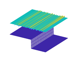
The numerical domain is shown in figure 1(b). Waves are generated using a double relaxation zone in order to fully absorb waves reflected back from the step. We mirror the directional wave generation set-up used in the experiment (i.e. linear summation of both random phase and random amplitude and also the single-summation method for the travelling direction of each wave component) to match the experimental input conditions and ensure the wave field is ergodic. We adopt the same underlying JONSWAP spectrum ( $\gamma =3.3$) and the same wrapped normal spreading function as the experiments. Waves are absorbed at the far end of the numerical domain. We use a spatial resolution of 0.068 m in the mean wave direction (approximately 31 nodes per peak wavelength on the deeper side) and 0.078 m in the transverse direction. We use a time discretisation of 0.03 s (approximately 41 steps per peak period) with a total simulation time of 2100 s for each case. The choice of spatial and temporal resolutions is based on the convergence study carried out by Li et al. (Reference Li, Tang, Draycott, Li, van den Bremer and Adcock2022b). We used fully reflective boundary conditions at the sidewall of the numerical domain to mirror the experimental set-up. We increase the domain sizes in the transverse direction for larger spreading sea states to ensure the reflected waves will have negligible effects in the region where we measure the statistics. A breaking criterion of the particle downward acceleration on the free surface exceeding $0.4g$ is adopted, where $g$ is the gravitational acceleration constant. When this breaking criterion is triggered, a local smoothing filter is applied on the free water surface and will extract a small amount of energy locally around the peak until the particle downward acceleration is below the threshold.
2.3. Limitations
Ideally, we would be able to compare identical parameters in the experiments and numerics. However, this is not possible due to experimental and numerical model limitations. The two key limitations are as follows. (i) We cannot test directional spreading values  $\theta _s$ of more than $5^{\circ }$ (see (2.2)) experimentally – this means that we have to compare experiments and numerics only over a limited range, a range we extend using numerics alone. (ii) We cannot simulate waves passing over a step with our numerical code but must use a steep slope instead. Li et al. (Reference Li, Tang, Draycott, Li, van den Bremer and Adcock2022b) found the code gave satisfactory results even for a near-vertical slope (15 : 1) although this required high resolution and had slightly greater numerical error than gentler slopes. Past work for unidirectional waves (e.g. Zheng et al. Reference Zheng, Lin, Li, Adcock, Li and van den Bremer2020) suggests that a 1 : 1 slope behaves almost identically to a step change in bathymetry (the change in depth occurs over roughly 0.1 of a wavelength on the deeper water side) and so we choose to use this for the present study.
There are, of course, other important issues with both physical and numerical experiments. Important ones for the present paper are that experimentally it is difficult to absorb waves (including those reflected back from the step to the paddle), whilst numerically a wave breaking model has to be applied which can only crudely capture the relevant physics.
3. Results
Owing to limitations of computational and experimental time, we have only varied the directional spreading and have not varied the geometry or other wave parameters. Geometrical details are shown in figure 1. The exact cases are shown in table 2. We vary the directional spreading from unidirectional through to  $30^{\circ }$, noting that spreading angles less than $15^{\circ }$ are unlikely for storm waves in the real ocean. For the five-degree case, two domain widths have been used – one matching the experiments and another matching the simulations for larger spreading. The results of these were carefully compared, and no significant differences were found. Thus these results are combined together for the results presented in this paper. This also gives reassurance that the rather narrow width of the domain relative to the length of the crest is not a significant source of error.
Figure 2 presents the variation of the significant wave height and kurtosis of the free surface as a function of  $x$. Kurtosis is a common proxy for rogue wave density (Mori & Janssen Reference Mori and Janssen2006). For an ideal linear sea, the value of the kurtosis is 3. These results are averaged over the width of the simulation for the numerics but measured along the centreline for the experiments. The significant wave height of the numerics shows a clear beating pattern before the step, which can be attributed to reflections off the depth discontinuity. After the depth change, there are only small variations in $H_s$ in the numerics, although there are significant differences, which are a function of the spreading angle. The experiments are in reasonable agreement with the numerics in the main region of interest. In the first metre after the step, they show a clear decline not captured in the numerics after this point, which may be due to depth-induced breaking not being accurately modelled numerically or, more probably, issues with reflections in experiments. Turning to kurtosis, we see the same general shape in both experiments and numerics, with a clear peak in kurtosis after the step consistent with the literature. Further down the domain, the kurtosis falls below 3, presumably due to shallow-water effects. The differences in magnitude are considered in more detail below.

Figure 2. Variation of significant wave height ( $H_s$) and kurtosis along the mean wave direction.
An alternative to kurtosis for analysing the number of extreme waves is to consider the exceedance probability of a given crest height. We analyse wave exceedance statistics from three locations at 0.25, 0.5 and 0.75 of the total tank width in the  $y$ direction, which helps the clarity of the statistical results. In figure 3(a), we present example exceedance probabilities at the gauge 0.8 m from the top of the depth discontinuity. We choose to analyse further the crest amplitudes at the $10^{-3.5}$ probability level (i.e. the amplitude exceeds by appropriately every 1 in 3200 waves), and trough amplitudes at $10^{-3}$ probability level. These are shown in figures 3(b)–3(d). Consistent with the kurtosis, both experiments and numerics predict a peak in the number of large crests after the depth decrease. However, the troughs show the opposite behaviour, with a clear minimum in the magnitude of the largest troughs. This is consistent with the model whereby the local change in wave statistics is due to the release of second-order bound waves, since these will tend to increase the size of crests and decrease that of troughs.

Figure 3. Wave crest and trough exceedance probabilities. (a,c) Example exceedance probabilities showing both experimental and numerical results at the  $x=0.8$ m gauge location for (a) the crests ( $\eta _c$) and (c) the troughs ( $\eta _t$), with the Rayleigh distribution given as reference. A zoomed-out plot is provided in each top-right corner, with dashed lines indicating exceedance of $10^{-3.5}$ for crests and $10^{-3}$ for troughs and the corresponding amplitude. (b) Crest amplitude at the $10^{-3.5}$ level along the $x$ direction for all cases. (d) Trough amplitude at the $10^{-3}$ level along the $x$ direction for all cases.
We now focus on the peak value of the kurtosis and peak crest height at the  $10^{-3.5}$ level. For the experiments, we present the largest of these at a gauge (i.e. we do not interpolate between gauges, so may miss the exact peak). Figure 4 presents these plotted against input directional spread. The trend is very similar for the numerics and experiments, with the largest peak in extreme waves occurring for unidirectional waves and the peaks decreasing as directional spread increases. However, there is a quantitative mismatch between the experiments and numerics. Interestingly, the kurtosis metric suggests that the numerics overpredicts the extreme waves whereas the crest statistics suggest the opposite. The same pattern is observable, although less clear, in figures 2 and 3.

Figure 4. Variation of peaks with directional spreading: (a) variation in the peak kurtosis observed; and (b) variation of largest  $10^{-3.5}$ exceedance probability with directional spreading.
4. Discussion
There is a significant mismatch between the experiments and numerics for the equivalent cases, with an overprediction of kurtosis but an underprediction of the largest crest. Whilst this inconsistency is surprising, the parameters are measuring different aspects of the extremes. However, there is clearly a difference between numerics and experiments, even if there is ambiguity about over- or underprediction. This discrepancy seems larger than that between experiments and the same code presented in Li et al. (Reference Li, Tang, Li, Draycott, van den Bremer and Adcock2023). There are obvious things that the potential flow code might capture poorly, such as wave breaking effects. However, we hypothesise that the cause of the discrepancy is due to issues with reflections in the tank, which were hard to suppress, and to differences in how the waves were generated, which effectively means that the incident sea state to the step was slightly different.
Despite this quantitative discrepancy, over the narrow spreading angles for which we have laboratory results, the trend is very similar between the experiments and numerical models. Given this, and the extensive work that has previously gone into showing that OceanWave3D can model the relevant physics, we have reasonable confidence in our numerical results and feel these are sufficient to draw, at least, a qualitative conclusion. This is that directionality inhibits, but does not stop, the mechanism which causes an excess of rogue waves at the top of slopes and that we predict this can occur for directional spreads relevant to waves in the real ocean.
There are several reasons why directionality might inhibit the mechanism by which rogue waves are made more likely by the presence of a step. Firstly, directionality reduces the magnitude of the second-order sum harmonic (at least for the range of values considered here). Thus, it is likely that the released wave will be smaller relative to the unidirectional case. Secondly, if there is a mismatch between the direction of propagation and the depth contours, then refraction will occur. This will be different for the primary wave and the released wave, meaning that the largest crest of each is less likely to coincide.
In the above discussion, we have assumed that the primary mechanism that produces the large waves is the release of bound waves (Li et al. Reference Li, Draycott, Adcock and van den Bremer2021a, Reference Li, Liang and Draycott2022a), although we note we do not directly observe this. It is likely that directionality will also have a significant impact on any amplification due to non-equilibrium, as directionality significantly alters the nonlinear wave–wave interactions, which must be key to any non-equilibrium mechanism.
5. Conclusion
Directional spreading reduces the number of rogue waves generated as waves pass over steps. Specifically, we find the number of rogue waves decreases as the directionality of a sea state increases. More cautiously, and based only on numerical modelling, we can say that this effect flattens off for directional spreads typically observed in storms in the ocean. Importantly, we still see significant amplification as directional waves pass over an abrupt depth transition. This appears to be consistent with the model, which indicates that this is caused by the release of incident bound waves as free waves as the wave propagates across the depth discontinuity (Li et al. Reference Li, Draycott, Adcock and van den Bremer2021a, Reference Li, Liang and Draycott2022a), although we note we do not directly observe this.
The obvious next steps are to extend theoretical models to account for directionality and to conduct directionally spread experiments for realistic values of spreading. Extensions to look at cases where the mean wave direction is not normal to the depth discontinuity would also be of interest.
Funding
T.T. is funded by an Eric and Wendy Schmidt AI in Science Postdoctoral Fellowship. S.D. acknowledges a Dame Kathleen Ollerenshaw Fellowship and thanks the EPSRC SuperGen Offshore Renewable Energy Hub (EP/S000747/1) for funding the experiments through the ECR Research Fund. This research was funded in whole or in part by EPSRC grant number EP/V050079/1. For the purpose of Open Access, the author has applied a CC BY public copyright licence to any Author Accepted Manuscript (AAM) version arising from this submission.
Declaration of interests
The authors report no conflict of interest.


 Open access