


1. Introduction
Bubble dynamics is a typical multiphase flow problem, which has received much attention for many years due to its broad applications and interesting behaviours (Prosperetti Reference Prosperetti2004; Lauterborn & Kurz Reference Lauterborn and Kurz2010; Lohse Reference Lohse2018). In most realistic circumstances, bubble dynamic behaviours are inevitably affected by boundary conditions of the flow field or external force fields such as gravity and acoustic waves (Lauterborn & Kurz Reference Lauterborn and Kurz2010; Supponen et al. Reference Supponen, Obreschkow, Tinguely, Kobel, Dorsaz and Farhat2016). Up to now many experimental, numerical and theoretical studies have been carried out of bubble dynamics near different boundaries, the most commonly seen of which are rigid walls (Blake, Taib & Doherty Reference Blake, Taib and Doherty1986; Zhang, Duncan & Chahine Reference Zhang, Duncan and Chahine1993; Hsiao et al. Reference Hsiao, Jayaprakash, Kapahi, Choi and Chahine2014; Wang Reference Wang2014; Beig, Aboulhasanzadeh & Johnsen Reference Beig, Aboulhasanzadeh and Johnsen2018), free surfaces (Chahine Reference Chahine1977; Wang et al. Reference Wang, Yeo, Khoo and Lam1996; Quah et al. Reference Quah, Karri, Ohl, Klaseboer and Khoo2018; Kang & Cho Reference Kang and Cho2019), elastic membranes (Sankin, Yuan & Zhong Reference Sankin, Yuan and Zhong2010), suspended structures (Goh et al. Reference Goh, Gong, Ohl and Khoo2017; Wu et al. Reference Wu, Zuo, Stone and Liu2017; Li et al. Reference Li, Zhang, Han and Ma2019a), adjacent bubbles (Tomita, Shima & Ohno Reference Tomita, Shima and Ohno1984; Bremond et al. Reference Bremond, Arora, Ohl and Lohse2006; Ochiai & Ishimoto Reference Ochiai and Ishimoto2017), etc. A significant diversity of bubble collapse patterns and jetting behaviours has been revealed. For instance, a high-speed liquid jet, an important destructive mechanism in cavitation and underwater explosions, is directed towards a rigid wall or away from a free surface (Blake & Gibson Reference Blake and Gibson1987; Philipp & Lauterborn Reference Philipp and Lauterborn1998; Kim et al. Reference Kim, Chahine, Franc and Karimi2014; Kiyama et al. Reference Kiyama, Shimazaki, Gordillo and Tagawa2021). We also benefit from bubble jets in some other applications, such as ultrasonic cleaning (Chahine et al. Reference Chahine, Kapahi, Choi and Hsiao2016; Reuter & Mettin Reference Reuter and Mettin2016), sonoporation (Ohl et al. Reference Ohl, Arora, Ikink, De Jong, Versluis, Delius and Lohse2006b; Kooiman et al. Reference Kooiman, Foppen-Harteveld, van der Steen and de Jong2011), printing (Turkoz et al. Reference Turkoz, Perazzo, Kim, Stone and Arnold2018), etc. In the majority of published literature, the flow field surrounding bubbles merely consists of a single type of fluid. The interaction between an oscillating bubble and the interface of two immiscible fluids is far from well understood, which has applications in ultrasonic emulsification (Canselier et al. Reference Canselier, Delmas, Wilhelm and Abismaïl2002), pharmacy (Freitas et al. Reference Freitas, Hielscher, Merkle and Gander2006), the food industry (Nishinari et al. Reference Nishinari, Fang, Guo and Phillips2014), sediment transport and dredging (Nielsen, Bach & Bollwerk Reference Nielsen, Bach and Bollwerk2015), ocean engineering (Xu et al. Reference Xu, Wang, Liu and Zhang2020), etc.
There have been a few experimental observations of bubble dynamics near a fluid–fluid interface. Chahine & Bovis (Reference Chahine and Bovis1980) performed experiments for spark-generated bubbles near the interface of two immiscible liquids. They discussed the dependence of the bubble jet direction on the standoff parameter and the Froude number since their motivation was cavitation damage reduction. Thereafter, this problem received little attention until very recently. Perdih, Zupanc & Dular (Reference Perdih, Zupanc and Dular2019) found rich phenomena occurred near the liquid–liquid interface which was exposed to ultrasonic cavitation, including cavitation bubble oscillation near the interface, penetration of a water jet into the bulk oil phase, breakup of oil droplets, etc. Yamamoto, Matsutaka & Komarov (Reference Yamamoto, Matsutaka and Komarov2021) experimentally studied the dynamics of acoustic cavitation bubbles near a gallium droplet interface. They partially demonstrated that a high-speed liquid jet from the bubble is the prime cause of liquid emulsification and a large amplitude of bubble oscillation is required to trigger a liquid jet. However, due to the limitations of spatio-temporal resolutions of such small-scale experiments ( ${\sim }100\ \mathrm {\mu }\textrm {m}$), the microscopic phenomena during the bubble–interface interaction are difficult to observe clearly. To better understand the fundamental ultrasonic emulsification process, Orthaber et al. (Reference Orthaber, Zevnik, Petkovšek and Dular2020) studied the jetting behaviour of a laser-induced cavitation bubble ( $\sim$1 mm) near a liquid–liquid interface. They found that the direction of the bubble jet is always from the lighter liquid to the denser liquid. The dependence of the bubble dynamics on an anisotropy parameter (Supponen et al. Reference Supponen, Obreschkow, Tinguely, Kobel, Dorsaz and Farhat2016) was also discussed. A similar bubble jet behaviour was also reported in the work of Yin et al. (Reference Yin, Huang, Tu, Gao and Bao2020). In the present work, the electric discharge method (Fong et al. Reference Fong, Adhikari, Klaseboer and Khoo2009; Cui et al. Reference Cui, Zhang, Wang and Khoo2018) is used to generate centimetre-scale cavitation bubbles, which allows us to achieve a higher spatio-temporal resolution of bubble dynamics and interface evolution than in earlier works. Additionally, three types of oils with different densities and viscosities are used in our experiments, aiming to provide new physical insights for bubble dynamics near a fluid–fluid interface.
There are also a few numerical studies of the interaction between a cavitation bubble and a fluid–fluid interface. Klaseboer & Khoo (Reference Klaseboer and Khoo2004b) established a boundary integral (BI) model for bubble–interface interactions based on the potential flow theory. The effects of the density ratio  $\alpha$ between two fluids were studied therein, including two limiting situations ( $\alpha \to 0$ and $\alpha = \infty$). The interface acts like a free surface and a rigid wall in these two situations, respectively. Curtiss et al. (Reference Curtiss, Leppinen, Wang and Blake2013) extended this model to study the interaction between a single ultrasound contrast agent type of bubble and a tissue layer. They found the inertial bubble provides an efficient way for removing polluted material layers by literally lifting them off an attached substrate. Rowlatt & Lind (Reference Rowlatt and Lind2017) adopted the spectral element marker particle method to study the bubble collapse near a fluid–fluid interface with applications in bioengineering. Liu et al. (Reference Liu, Zhang, Tian and Wang2019) proposed a volume of fluid model implemented in the finite element method to study the behaviour of a bubble generated at the interface of two different liquids. They revealed the role of gravity and density ratio of the two fluids in bubble migration and jet direction. The same method was also applied to study the bubble–seabed interaction in shallow water (Xu et al. Reference Xu, Wang, Liu and Zhang2020). Yamamoto & Komarov (Reference Yamamoto and Komarov2020) numerically studied the jet dynamics of acoustic cavitation bubbles near a gallium droplet using a commercial software. They found that the jet velocity of the bubble is maximized at a moderate initial bubble–interface distance.
Most of the aforementioned experimental and numerical studies were restricted to bubble dynamics on a short time scale; however, we have little knowledge of the residual flow after bubble collapse, i.e. the dynamics of the interface jet on a much longer time scale. To fill this knowledge gap, both the bubble dynamics and the interface jet evolution on multiple time scales are investigated in this study. Remarkably, besides the penetration of a high-speed bubble jet into the fluid–fluid interface, the pinch-off of an interface jet also leads to the mixing of fluids. The dependence of the associated fluid dynamics on the governing parameters is systematically studied via experiments, BI simulations and a scaling analysis.
This paper is structured as follows. In § 2, we present our experimental set-up and numerical model. In § 3, the general physical phenomena are discussed for bubble initiations in different fluids or at the interface. In § 4, the experimental observations are compared with BI simulations or theoretical results from an extended Rayleigh–Plesset model. In § 5, a quantitative study is presented for bubble jet dynamics. In § 6, the dependence of the interface jet dynamics on governing parameters is discussed. Finally, this work is summarized and conclusions are drawn in § 7.
2. Methodology
2.1. Experimental set-up
An underwater electric discharge method (Turangan et al. Reference Turangan, Ong, Klaseboer and Khoo2006; Cui et al. Reference Cui, Zhang, Wang and Khoo2018) is adopted to generate cavitation bubbles in our experiments. Two copper-alloy wires with a diameter of  $\sim$0.2 mm cross and touch at a point, which is the initial centre of the bubble. At first, a capacitor is charged to 500 V. Upon discharge, strong Joule heating at the crossing point vaporizes the surrounding water or oil, and a centimetre-scale bubble is thus generated. The maximum radius of the bubble is around 15 mm. Details of the bubble generator can be found in our previous studies (Cui et al. Reference Cui, Zhang, Wang and Khoo2018). Although the bubble is a result of local heating and boiling, it is still called a ‘cavitation bubble’ in the community of bubble dynamics since the basic mechanics of cavitation and boiling is similar and the main content is vapour (Kling & Hammitt Reference Kling and Hammitt1972; Blake & Gibson Reference Blake and Gibson1987; Brennen Reference Brennen1995). Though cold boiled water and oils are used in the experiment, we still find that a small amount of non-condensable gas slowly enters the bubble due to diffusion.
Experiments are performed in a water tank of  $300\ \textrm {mm}\times 300\ \textrm {mm}\times 600\ \textrm {mm}$ under atmospheric pressure and at room temperature ( ${\sim }20\,^{\circ }\textrm {C}$). The tank is firstly filled with water to 300 mm in depth and then the oil is added gently and slowly to 280 mm in depth. An oil–water interface is thus formed between the two immiscible fluids. To gain better insight into the interaction between bubbles and the oil–water interface, we use three types of oils in the experiments and their physical properties are given in table 1. Besides, the density and viscosity of water in our experiment are $0.999\ \textrm {g}\ \textrm {cm}^{-3}$ and $0.001\ \textrm {Pa}\ \textrm {s}$, respectively. The initial centre of a cavitation bubble is arranged near or at the interface and the strong interaction is experimentally studied in a systematic manner. A continuous light source provides illumination from the back. A high-speed camera (Phantom V711) is triggered at the same time with a discharge switch. Both the transient bubble behaviours and the interface evolutions on a longer time scale are well captured by the camera working at 16 000–21 000 frames per second with an exposure time of $10\ \mathrm {\mu }\textrm {s}$. The temporal resolution ( $47.6 - 62.5\ \mathrm {\mu }\textrm {s}$) is within 2 % of the first period of bubble oscillation and 0.1 % of the interface jet evolution process. The uncertainty of the length measurement can be estimated as one pixel of the image (0.1 to 0.2 mm), which is around 1 % of the maximum bubble radius.
Table 1. The properties of three types of oil used in the experiments.

The bubble–interface interactions in our experiments are inertia-controlled on a small time scale and the viscosity effects are negligible (see further explanation in § 3.1). For micrometre-sized ultrasonic bubbles in some practical applications, the key physical process is usually accompanied by an energetic collapse and a high-speed liquid jet. For instance, a large amplitude of bubble oscillation is an essential condition for emulsification (Yamamoto et al. Reference Yamamoto, Matsutaka and Komarov2021); the jet impact plays a vital role in removing unwanted material layers on a surface (Ohl et al. Reference Ohl, Arora, Dijkink, Janve and Lohse2006a; Curtiss et al. Reference Curtiss, Leppinen, Wang and Blake2013). The associated Reynolds numbers are still much larger than 1. Therefore, it is convincing that our experimental data can shed light on the behaviour of micrometre-sized cavitation bubbles. For a much longer time scale, the interface evolution in our system is determined by the competing effects of inertia, surface tension, gravity and viscosity, which may also provide insights into the essential physics of problems at the micrometre scale.
2.2. Numerical model
A sketch of the physical problem is shown in figure 1. A relatively heavy fluid (fluid 1, water) and a second fluid (fluid 2, oil) are separated by a sharp fluid–fluid interface. An axisymmetric BI method is used to simulate the interaction between a cavitation bubble and the fluid–fluid interface. We define a cylindrical coordinate  $O$–
$O$– $r\theta z$ with the origin $O$ located at the fluid–fluid interface, vertically above or below an initially spherical bubble. The distance between the initial bubble centre ( $0, 0, z_b$) and the interface is denoted by $d_b$.

Figure 1. Schematic diagram for the interaction between a cavitation bubble and a fluid–fluid interface (a) at the initiation time and (b) in the bubble expansion stage.
In the following introduction of the model, we suppose the bubble is initiated in fluid 1. One can easily extend the model to the situation of bubble initiation in fluid 2. According to the work of Klaseboer & Khoo (Reference Klaseboer and Khoo2004a), Gordillo et al. (Reference Gordillo, Sevilla, Rodríguez-Rodríguez and Martínez-Bazán2005) and RodríGuez-RodríGuez, Gordillo & Martínez-Bazán (Reference RodríGuez-RodríGuez, Gordillo and Martínez-Bazán2006), fluid 1 and fluid 2 are considered as inviscid and incompressible. The Laplace equation is valid in both fluids and the velocity potentials  $\varphi _1$ and $\varphi _2$ satisfy the BI equation, written as
 \begin{gather} \nabla^2{\varphi_i}=0\quad (i=1,2), \end{gather}
 \begin{gather}c(\boldsymbol{{r}})\varphi_i(\boldsymbol{{r}})=\iint_S\left(\frac{\partial \varphi_i(\boldsymbol{{q}})} {\partial n}\frac{1}{\left| \boldsymbol{{r}}-\boldsymbol{{q}}\right| }-\varphi_i (\boldsymbol{{q}})\frac{\partial}{\partial n}\left(\frac{1}{\left| \boldsymbol{{r}}-\boldsymbol{{q}}\right| }\right) \right) \textrm{d}S_i(\boldsymbol{{q}})\quad (i=1,2), \end{gather}
where  $c$ denotes the solid angle, $\boldsymbol{ {r}}$ and $\boldsymbol{ {q}}$ the control and source points, respectively, and $\partial /\partial n$ the normal derivative. Here $S$ refers to the fluid–fluid interface and the bubble surface when $i = 1$ (flow domain 1), while it refers to the fluid–fluid interface only when $i = 2$ (flow domain 2).
The dynamic boundary conditions on the bubble surface and at the fluid–fluid interface can be written as
 \begin{gather} \frac{{\partial}{\varphi_1}}{{\partial}t}=\frac{P_{\infty}}{\rho_1}-\frac{P_{L}}{\rho_1}-\frac{1}{2}{|{\boldsymbol{\nabla} \varphi_1}|^2}-g(z+z_b)\quad \text{on the bubble surface}, \end{gather}
 \begin{gather}\frac{{\partial}{\varphi_1}}{{\partial}t}=\frac{P_{\infty}}{\rho_1}-\frac{P_{1}}{\rho_1}-\frac{1}{2}{|{\boldsymbol{\nabla} \varphi_1}|^2}-gz\quad {\text{at the interface}}, \end{gather}
 \begin{gather}\frac{{\partial}{\varphi_2}}{{\partial}t}=\frac{P_{\infty}}{\rho_2}-\frac{P_{2}}{\rho_2}-\frac{1}{2}{|{\boldsymbol{\nabla} \varphi_2}|^2}-gz\quad {\text{at the interface}}, \end{gather}
where  $P_\infty$ is the hydrostatic pressure at $z=0$, $P_L$ the liquid pressure on the bubble surface, $P_1$ and $P_2$ the pressures just below and above the interface, respectively, $\rho$ the density of the fluid and $g$ the gravitational acceleration. With the material derivative $\textrm {D}/\textrm {D}t=\partial /\partial t+\boldsymbol {\nabla } \varphi _1\boldsymbol {\cdot }\boldsymbol {\nabla }$, (2.3), (2.4) and (2.5) transform into
 \begin{gather} \frac{\textrm{D}{\varphi_1}}{\textrm{D}t}=\frac{P_{\infty}}{\rho_1}-\frac{P_{L}}{\rho_1}+\frac{1}{2}{|{\boldsymbol{\nabla} \varphi_1}|^2}-g(z+z_b)\quad \text{on the bubble surface}, \end{gather}
 \begin{gather}\frac{\textrm{D}{\varphi_1}}{\textrm{D}t}=\frac{P_{\infty}}{\rho_1}-\frac{P_{1}}{\rho_1}+\frac{1}{2}{|{\boldsymbol{\nabla} \varphi_1}|^2}-gz\quad \text{at the interface}, \end{gather}
 \begin{gather}\frac{\textrm{D}{\varphi_2}}{\textrm{D}t}=\frac{P_{\infty}}{\rho_2}-\frac{P_{2}}{\rho_2}+\boldsymbol{\nabla} \varphi_1\boldsymbol{\cdot}\boldsymbol{\nabla} \varphi_2-\frac{1}{2}{|{\boldsymbol{\nabla} \varphi_2}|^2}-gz\quad \text{at the interface}. \end{gather}
 Taking the surface tension into account, the relation between the internal pressure of the bubble  $P_b$ and the liquid pressure $P_L$ on the bubble surface satisfies
 \begin{equation} P_b=P_0\left(\frac{V_0}{V}\right) ^{\lambda}=P_{L}+\sigma\kappa,\end{equation}
where the subscript ‘0’ represents initial quantities and  $V$ is the bubble volume, $\lambda$ the ratio of the specific heats, $\sigma$ the surface tension coefficient and $\kappa$ the local curvature. For simplicity, here we use the adiabatic approximation to model the gas pressure inside the bubble, as suggested by Klaseboer, Turangan & Khoo (Reference Klaseboer, Turangan and Khoo2006), Lee, Klaseboer & Khoo (Reference Lee, Klaseboer and Khoo2007) and others. For the bubble dynamics in our experiments, the associated Péclet number (defined as $R_{m}^2/T_{osi}D$, where $R_{m}$ is the maximum bubble radius, $T_{osi}$ the bubble period and $D$ the thermal diffusivity) can be estimated as $O(10^3)$, which justifies the adiabatic assumption.
Substituting (2.9) into (2.6), the dynamic boundary condition on the bubble surface is thus obtained as follows:
 \begin{equation} \frac{\textrm{D}{\varphi_1}}{\textrm{D}t}=\frac{P_{\infty}}{\rho_1}-\frac{P_{0}}{\rho_1}\left(\frac{V_0}{V} \right) ^\lambda+\frac{\sigma \kappa}{\rho_1}+\frac{1}{2}{|{\boldsymbol{\nabla} \varphi_1}|^2}-g(z+z_b).\end{equation}
At the water–oil interface, the condition on the normal stresses is given by
 \begin{equation} P{_2}=P_1+\sigma \kappa-2\mu_2\frac{\partial^2\varphi_2}{\partial n^2},\end{equation}
where  $\mu _2$ is the oil viscosity and the last term denotes the normal viscous stress. Here we ignore the water viscosity since its value is much smaller than that of the oil. The theory of viscous potential flow works well when vorticity is restricted to a thin layer near the boundary (Joseph & Wang Reference Joseph and Wang2004; Klaseboer et al. Reference Klaseboer, Manica, Chan and Khoo2011). Some justification is given in § 4.1.
From (2.7), (2.8) and (2.11), the dynamic boundary condition at the interface is obtained as follows:
 \begin{equation} \frac{\textrm{D}{(\varphi_1-\alpha\varphi_2)}}{\textrm{D}t}=\frac{1}{2}{|{\boldsymbol{\nabla} \varphi_1}|^2}+\frac{\alpha}{2}{|{\boldsymbol{\nabla} \varphi_2}|^2}-\alpha\boldsymbol{\nabla}\varphi_1\boldsymbol{\cdot}\boldsymbol{\nabla}\varphi_2-(1-\alpha)gz+\frac{\sigma \kappa}{\rho_1}-2\frac{\mu_2}{\rho_1}\frac{\partial^2\varphi_2}{\partial n^2},\end{equation}
where  $\alpha =\rho _2/\rho _1$ is defined as the density ratio.
The kinematic boundary condition on all surfaces is given by
 \begin{equation} \frac{\textrm{D}{\boldsymbol{{r}}}}{\textrm{D}t}=\boldsymbol{\nabla}\varphi_1.\end{equation}
 If a cavitation bubble is initiated in oil (fluid 2), (2.12) can be deduced in the same manner with the material velocity  $\boldsymbol{ {u}}_2=\boldsymbol {\nabla }\varphi _2$.
Although the above derivation process is similar to that in Klaseboer & Khoo (Reference Klaseboer and Khoo2004a,Reference Klaseboer and Khoob), the interaction between a toroidal bubble (after the jet impact) and the interface was not considered with therein. In this study, the interaction between a toroidal bubble and the interface is numerically investigated using a vortex ring model (Wang et al. Reference Wang, Yeo, Khoo and Lam1996). The velocity potential  $\varphi$ is decomposed into two parts, i.e. the potential due to the circulation of the vortex ring $\varphi _{vor}$, which is obtained using a semi-analytical method (Zhang, Li & Cui Reference Zhang, Li and Cui2015), and the remnant potential $\varphi _{res}$. The induced velocity of the vortex ring is calculated using the Biot–Savart law, while the remnant velocity is calculated from the BI equation (2.2). For details of the vortex ring model for simulating the toroidal bubble motion, the reader is referred to the work of Wang et al. (Reference Wang, Yeo, Khoo and Lam1996) and Zhang et al. (Reference Zhang, Li and Cui2015).
2.3. Non-dimensionalization and initialization
In the present study, numerical calculations are performed in a dimensionless system. The equivalent maximum radius of the bubble  $R_m$, the hydrostatic pressure at the initial interface $P_\infty$ and the density of the heavier fluid $\rho _1$ are used as three basic quantities to convert other parameters into dimensionless quantities. Four dimensionless variables are introduced as follows:
 \begin{equation} \gamma=\frac{d_b}{R_m},\quad \alpha=\frac{\rho_2}{\rho_1},\quad \varepsilon=\frac{P_0}{P_\infty},\quad \delta=\sqrt{\frac{\rho gR_m}{P_\infty}}, \end{equation}
where  $\gamma$ is defined as the standoff parameter, $\alpha$ the density ratio, $\varepsilon$ the strength parameter and $\delta$ the buoyancy parameter (equivalent to the inverse Froude number). For convenience, we denote $\gamma _w$ and $\gamma _o$ as the standoff parameter for bubble initiations in water (denser fluid) and oil (lighter fluid), respectively.
To match the experiment, the initial conditions should be set properly in numerical simulations. In the experiment, the discharge process lasts for about 0.3 ms (about one-tenth of the first cycle of the bubble); thus the electric energy is not transferred to the bubble immediately. Up until now, to the best knowledge of the authors, no successful attempt has been made to model the early stage of an electric discharge bubble. Following published literature (Tong et al. Reference Tong, Schiffers, Shaw, Blake and Emmony1999; Klaseboer et al. Reference Klaseboer, Hung, Wang, Wang, Khoo, Boyce, Debono and Charlier2005; Hsiao et al. Reference Hsiao2013; Zeng et al. Reference Zeng, Gonzalez-Avila, Dijkink, Koukouvinis, Gavaises and Ohl2018), we use a simplified method to initialize the bubble in simulations, namely the bubble is set as an initially stationary high-pressure gas bubble. The Rayleigh–Plesset equation (Plesset Reference Plesset1949) in a non-dimensional form,
 \begin{equation} R\ddot{R}+\frac{3}{2}\dot{R}^2=\varepsilon\left(\frac{R_0}{R} \right) ^{3\lambda}-1,\end{equation}
is used to fit the free-field experiment by adjusting the initial bubble radius  $R_0$ and the strength parameter $\varepsilon$. Since the dimensionless maximum bubble radius is 1, the relationship between $R_0$ and $\varepsilon$ (Klaseboer et al. Reference Klaseboer, Hung, Wang, Wang, Khoo, Boyce, Debono and Charlier2005) can be derived from the energy conservation law:
 \begin{equation} \frac{\varepsilon}{\lambda-1}(R_0^{3\lambda}-R_0^3)=R_0^3-1.\end{equation}
 Since the content of the bubble is vapour and a small amount of diffused air, the ratio of the specific heats  $\lambda$ should be less than 1.4. However, it is difficult to measure the exact value. Fortunately, the bubble dynamics is not sensitive to the choice of $\lambda$; for example, the bubble oscillation period $T_{osi}$ only varies ${\sim }3\ \%$ when $\lambda$ ranges from 1.2 to 1.4 (not shown here). Hence, we set $\lambda =1.25$ in this study according to Lee et al. (Reference Lee, Klaseboer and Khoo2007), Fong et al. (Reference Fong, Adhikari, Klaseboer and Khoo2009) and Gong et al. (Reference Gong, Ohl, Klaseboer and Khoo2010). Now we only need to adjust the strength parameter $\varepsilon$ to fit the experimental data and the initial bubble radius is calculated from (2.16). The experimental data of the bubble radius evolution in a free field are compared with theoretical predications from (2.15) with different $\varepsilon$, as shown in figure 2. Four experiments are presented, including bubble initiations in sunflower oil and water. In the simulations, four different $\varepsilon$ are chosen, namely 50, 100, 200 and 400. Discrepancies between the experimental and theoretical results are noted in the expansion phase, which are mainly due to the fact that the bubble energy is gradually increased during the discharge process in the experiments. Nevertheless, after the bubble reaches the maximum volume, the experimental data start to follow the theoretical results when $\varepsilon$ is set between 100 and 200. The $\varepsilon =50$ simulation overestimates $T_{osi}$ while the $\varepsilon =400$ simulation underestimates $T_{osi}$. The inset also illustrates the dependence of $T_{osi}$ on $\varepsilon$. A satisfactory result can be obtained if $\varepsilon$ is chosen within the red dotted lines. Therefore, the initial non-dimensional pressure and radius of the bubble are set as $\varepsilon =100$ and $R_0 = 0.1485$ in this study. Dozens of experiments have been performed in a free field and the difference in $T_{osi}$ between experimental and theoretical results is within 2.3 %, which also proves the good reproducibility of the present experimental set-up. Finally, we emphasize that the time evolutions of the scaled bubble radius nearly collapse together, indicating that the viscosity of the oil plays a minor role in bubble oscillations of our present system.

Figure 2. Comparison of experimental data and theoretical results for dimensionless bubble radius evolution in a free field. The first two experiments are conducted in sunflower oil and the other two experiments in water. Four theoretical results (obtained using the Rayleigh–Plesset (RP) equation) are given for different  $\varepsilon$. In the inset, the solid black line denotes the dependence of the calculated bubble oscillation period on $\varepsilon$ and the two red dotted lines show the range of $T_{osi}$ in experiments. The time is scaled by $R_m\sqrt {\rho /P_\infty }$.
3. General physical phenomena
Firstly, we present and discuss several representative experimental results for bubbles initiated in water, in oil and at the interface. The dependence of the overall physical phenomena on the standoff parameter is qualitatively studied. In this section, only the sunflower oil is used.
3.1. Bubble initiation in water
In figure 3, four representative experiments are shown with a decreasing standoff parameter  $\gamma _w$. This allows us to anticipate an increase in the interaction between the bubble and the water–oil interface. In the first experiment (see figure 3a), the standoff parameter is $\gamma _w=1.32$ and the corresponding bubble–interface interaction is relatively weak. The bubble expands rapidly after inception (frames 1–3) and the interface elevates slightly with bubble expansion. The maximum amplitude of the interface motion is reached when the bubble attains the maximum volume (frame 3). The interface descends with the contraction of the bubble (frame 4) and almost recovers its initial shape when the bubble attains its minimum volume (frame 5). We note that the bubble keeps a spherical shape during the first oscillation cycle, indicating that the bubble is little influenced by the presence of the upper interface. In frame 6, the bubble rebounds to its maximum volume during the second cycle and we can hardly observe perturbations at the water–oil interface. The remaining energy of the bubble in the second cycle is only 16 % of that of the first cycle, which is estimated from the maximum bubble volume (Lee et al. Reference Lee, Klaseboer and Khoo2007). Thereafter, the bubble oscillates for several cycles with a damping amplitude, accompanied by a downward migration of the bubble centroid (frame 7). On a much longer time scale, the interface rises very slowly (frames 8–9) and the maximum height of the interface is reached at $t=101.92$ (frame 10). When $\gamma _w \gtrsim 1.32$, this residual flow at the interface cannot be observed in our experiments. It is noted that the cavitation bubble eventually turns into some non-condensable gas bubbles due to diffusion (Moreno Soto et al. Reference Moreno Soto, Maddalena, Fraters, van der Meer and Lohse2018). The average volume of the non-condensable gas is about 0.33 ml. Subsequently, these rising gas bubbles pass through the water–oil interface, which is beyond the scope of this study.

Figure 3. Four representative experiments of bubble–interface interaction for  $\gamma _w=1.32$, 0.91, 0.58 and 0.42, respectively. In all the sequences the bubble is initiated in water. (a) The bubble–interface interaction is weak and the bubble keeps a spherical shape during the first cycle ( $R_m=14.5\ \textrm {mm}$, $z_b=-19.1\ \textrm {mm}$). (b) A downward liquid jet forms during the rebound phase. The interface shows a simple smooth hump ( $R_m=14.4\ \textrm {mm}$, $z_b=-13.1\ \textrm {mm}$). (c) A downward liquid jet forms around the moment of the minimum bubble volume and a pronounced interface jet forms afterwards ( $R_m=15.9\ \textrm {mm}$, $z_b=-9.2\ \textrm {mm}$). (d) The bubble–interface interaction is strong and interface jet shows an annular neck above the half-height position ( $R_m=13.0\ \textrm {mm}$, $z_b=-5.5\ \textrm {mm}$). In this and subsequent figures, the dimensionless times are marked at the lower right corners. The time scales are 1.42, 1.41, 1.56 and 1.27 ms, respectively. The width of each frame is 40 mm. For results regarding the first bubble cycle in (b–d), the reader is referred to Appendix B.
In the second experiment (see figure 3b),  $\gamma _w$ is decreased to 0.91. The first cycle of the bubble is not given here (the reader is referred to Appendix B). Frame 1 shows the rebounding bubble in the early second cycle. A thin liquid jet can be seen inside the toroidal bubble, which implies that the bubble–interface interaction becomes stronger compared to the previous case. Additionally, the downward migration of the bubble is faster and the interface shows a simple smooth hump in the later stage (frames 3–5). It takes longer for the interface to reach its maximum height ( $t=117.78$, frame 5). In the third experiment (see figure 3c), $\gamma _w=0.58$. A downward liquid jet forms around the moment of the minimum bubble volume (not shown here). An annular neck can be seen on the toroidal bubble surface during the rebound phase (frame 1). After the bubble migrates away from the interface, the interface rises quickly (frame 2) and the interface jet grows much higher than in the previous two cases (frames 3–5). The maximum dimensionless height of the interface jet $h_m$ is around 1.32. In the fourth experiment, $\gamma _w$ is further reduced to 0.42. The toroidal bubble is more elongated along the axis of symmetry during the rebound phase (frame 1), indicating that the downward liquid jet of the bubble is more energetic. On a longer time scale, the interface jet is no longer a smooth hump; instead it shows an annular neck above the half-height position (frames 2–4). However, this neck disappears in the later stage (frame 5).
To understand the governing factors that influence the bubble dynamics and interface jet evolution, we first look at the associated dimensionless numbers. For the bubble dynamics on a short time scale ( ${\sim }T_{osc}$), the associated Reynolds number and Weber number can be defined as
 \begin{equation} Re=\frac{\rho R_m U}{\mu}\sim O(10^5),\quad We=\frac{\rho U^2 R_m}{\sigma}\sim O(10^4), \end{equation}
where the characteristic velocity is taken as  $U=\sqrt {P_\infty /\rho }\approx 10\ \textrm {m}\ \textrm {s}^{-1}$. Here we use the water viscosity $\mu _1=10^{-3}\ \textrm {Pa}\ \textrm {s}$ and surface tension $\sigma =0.073\ \textrm {N}\ \textrm {m}$ in (3.1a,b). This illustrates that the liquid viscosity and surface tension play a minor role during the bubble–interface interaction on a short time scale. This statement will be further confirmed by our numerical simulation. However, for the long-time evolution of the interface jet, the characteristic velocity should be replaced by a new one, namely the average rising velocity of the interface jet $\bar {U}=h_m/T_m$, where $T_m$ is the time for the interface to reach its maximum height. In the four experiments discussed above, $0.01\ \textrm {m}\ \textrm {s}^{-1}<\bar {U}< 0.14\ \textrm {m}\ \textrm {s}^{-1}$. The characteristic length remains the same since the interface jet has a size comparable with that of the bubble. The oil viscosity $\mu _2=62\times 10^{-3}\ \textrm {Pa}\ \textrm {s}$ is used. Thus we can obtain another Reynolds number and Weber number:
 \begin{equation} Re^*\sim O(10^0-10^1),\quad We^*\sim O(10^{-1}-10^1). \end{equation}
This implies that both the viscosity and surface tension come into play during the long-time evolution of the interface jet. Additionally, we use the Bond number
 \begin{equation} Bo=(\rho_1-\rho_2)gR_m^2/\sigma \end{equation}
to estimate the ratio of buoyancy to capillarity. In the four experiments discussed above,  $Bo\approx 7$; thus both gravity and surface tension are important in the growth and descent of the interface jet.
In the experiments discussed above, we find that the interface evolution is closely related to the bubble motion during the first cycle of the bubble. More specifically, the interface is pushed away by the expanding bubble and attracted by the collapsing bubble, which is different from that in bubble interactions with a water–air interface (Blake & Gibson Reference Blake and Gibson1987; Koukouvinis et al. Reference Koukouvinis, Gavaises, Supponen and Farhat2016; Kang & Cho Reference Kang and Cho2019). The inertia of the air is much smaller than that of water and the pressure at the interface nearly remains at atmospheric pressure. For small standoff parameters, the water–air interface is continuously pushed upward during the whole bubble life, generating a pronounced interface spike (Chahine Reference Chahine1977; Wang et al. Reference Wang, Yeo, Khoo and Lam1996; Koukouvinis et al. Reference Koukouvinis, Gavaises, Supponen and Farhat2016; Kang & Cho Reference Kang and Cho2019). Additionally, bubble bursting would occur if the bubble is very close to the water–air interface (i.e.  $\gamma _f\lesssim 0.5$) (Li et al. Reference Li, Zhang, Wang, Li and Liu2019b). In the present system, however, despite the small dimensionless standoff parameter in the fourth case ( $\gamma _w=0.42$), there is always a thin film between the bubble and the interface, and different interface jet dynamics are thus obtained.
Nevertheless, previous work on bubble interactions with a water–air interface stimulates us to give a similar mechanical explanation of the interface jet in the context of the conservation of linear momentum via a quantity of Kelvin impulse (Blake & Gibson Reference Blake and Gibson1987; Blake, Leppinen & Wang Reference Blake, Leppinen and Wang2015; Kang & Cho Reference Kang and Cho2019). As shown in figure 3, a long-lasting downward-moving bubble can be observed after the first collapse phase, which induces a downward fluid motion of a ‘virtual/added mass’ (Benjamin & Ellis Reference Benjamin and Ellis1966; Philipp & Lauterborn Reference Philipp and Lauterborn1998). Thus, a portion of fluid is expected to move in the opposite direction to bubble migration. One can also readily understand this using Newton's third law. Specifically, the bubble propels itself downward by pushing a certain amount of fluid upwards in the form of an interface jet. The above argument is justified by a scaling analysis in § 6 and a more quantitative discussion is given.
3.2. Bubble initiation at the water–oil interface
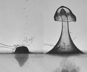
In this section, we discuss a special case, i.e. the initiation point of the bubble is positioned at the interface ( $\gamma =0$). As shown in figure 4, both the upper half and lower half of the bubble expand hemispherically (frames 1–2), while the different densities of the two fluids lead to different velocities of the upper and lower parts of the bubble (frame 3). Finally, a downward jet forms due to the faster contraction of the upper part, carrying some oil into the water through the interface (frame 4), which is a direct consequence of the lower inertia of the oil. Yamamoto et al. (Reference Yamamoto, Matsutaka and Komarov2021) supposed that such a bubble jet is an important mechanism in ultrasonic emulsification; however, no clear evidence was provided therein due to limitations of spatio-temporal resolutions. As shown in frame 5, a subsequent fast migration of the toroidal bubble in the rebound phase is observed. Presumably, the whole bubble is fully submerged in water at this moment. Owing to the significant influence of the bubble on the interface motion, the interface jet forms earlier and rises more quickly compared with the four cases considered in figure 3. The interface evolution on a longer time scale is presented in frames 6–10. A mushroom-shaped jet is gradually formed (frames 6–7). Subsequently, its cap grows and forms a stretching water film; meanwhile, the jet becomes thinner and thinner (frame 8). Afterwards, the interface jet splits into two parts, i.e. the cap and the lower part (frames 9–10). The very distorted cap turns into an ellipsoidal one due to surface tension (frame 10). It takes much longer for the water droplets to fall down to the interface (not given here). This finding may be the second mechanism of fluid mixing in ultrasonic emulsification. Different from the first mechanism, the second one transports the heavier fluid into the lighter fluid. Additionally, the pinch-off droplet is much larger than the oil droplets carried by the bubble jet; thus these two mechanisms may play a role in different stages of emulsification.

Figure 4. Bubble initiation at the water–oil interface. Frames 1–5 show the bubble dynamics on a short time-scale. Frames 6–10 show the interface evolution and the pinch-off of the interface jet. Here  $R_m=15.4\ \textrm {mm}$, $z_b=0$. The time scale is 1.52 ms. The width of each frame is 40 mm.
A similar experimental observation can be found in Yin et al. (Reference Yin, Huang, Tu, Gao and Bao2020) (see figure 9 therein). The difference is that their laser-induced cavitation bubble is one order of magnitude smaller than ours and the associated  $Bo$ is smaller than 1. Thus the effect of surface tension dominates over the effect of gravity in their system. Later we discuss the dependence of the interface jet dynamics on $Bo$ via numerical simulations.
3.3. Bubble initiation in oil
In figure 5, we present and discuss four representative experiments in which bubbles are generated in the sunflower oil, also starting with a large standoff parameter  $\gamma _o$. In the first experiment (see figure 5a), $\gamma _o=1.27$. The bubble oscillates spherically in the first cycle and no evident liquid jet can be seen (the reader is referred to Appendix B for the bubble dynamics in the first cycle). Only a tiny protrusion can be observed at the bottom of the bubble surface during the rebound phase (frame 1). Frame 2 shows the maximum volume of the bubble in the second cycle. Subsequently, the bubble oscillates for several cycles and migrates towards the interface very slowly (frames 3–4). The bubble only causes some deformation of the interface and no penetration occurs. In frame 5, non-condensable gas bubbles are rising above the water–oil interface. Below this standoff parameter $\gamma _o\approx 1.27$, we find that the bubble can penetrate the water–oil interface.

Figure 5. Four representative experiments of bubble–interface interaction for  $\gamma _o=1.27$, 1.2, 0.8 and 0.4, respectively. In all the sequences the bubble is initiated in oil. (a) The bubble only causes some deformation of the interface and no penetration occurs ( $R_m=13.4\ \textrm {mm}$, $z_b=17.0\ \textrm {mm}$). (b) A downward liquid jet forms during the rebound phase of the bubble. The bubble can pass through the water–oil interface on a much longer time scale ( $R_m=14.8\ \textrm {mm}$, $z_b=17.8\ \textrm {mm}$). (c) The downward bubble jet directly impacts and penetrates the interface ( $R_m=14.6\ \textrm {mm}$, $z_b=11.7\ \textrm {mm}$). (d) The bubble jet penetrates quite deep into the water and a mushroom-shaped interface jet forms ( $R_m=13.9\ \textrm {mm}$, $z_b=5.6\ \textrm {mm}$). The time scales are 1.26, 1.40, 1.37 and 1.31 ms, respectively. The width of each frame is 40 mm.
In the second experiment shown in figure 5(b),  $\gamma _o$ is reduced to 1.2. A sharp downward protrusion forms at the bottom of the bubble (frame 1), indicating the formation of a liquid jet. However, the jet tip cannot reach the position of the interface before disintegrating (frame 2). Though the bubble energy dissipates much after multiple oscillations, the downward-migrating bubble eventually passes through the water–oil interface (frames 3–5), resulting in a strong mass transport between the oil and water. No evident interface jet can be observed in this case.
In the third experiment shown in figure 5(c),  $\gamma _o=0.8$. The downward bubble jet directly impacts and penetrates the interface (frames 1–2). More discussion of bubble jet dynamics is given in § 5. Thereafter, the whole bubble passes through the water–oil interface and further migrates downward (frame 3). Remarkably, a pronounced interface jet is generated but no necking or pinch-off occurs (frames 4–5).
In the fourth experiment shown in figure 5(d), the bubble is initiated very close to the interface, i.e.  $\gamma _o=0.4$. The bubble jet penetrates deeper into the water compared to the third experiment (frame 1). When the bubble rebounds to the maximum size (frame 2), more than half of the bubble enters the water. As the bubble re-collapses and continually migrates downward, it quickly becomes fully submerged in the water bulk (frame 3). As expected, an interface jet is produced afterwards (frame 4). The jet tip assumes a mushroom shape and the cap finally separates from the main jet (frame 5). We can compare this case with that in figure 3(d). Despite a similar standoff parameter in these two experiments, the interface jet in the current experiment case grows faster and finally the pinch-off occurs; while in the former case, the interface jet grows more slowly and only a necking phenomenon is observed. We explain this as follows. When a bubble is initiated in water, the bubble migrates away from the interface and thus the subsequent bubble–interface interaction is weakened. For a bubble initiated in oil, the bubble migrates towards the interface and gradually passes through the interface, leading to a stronger bubble–interface interaction.
4. Comparison of experiments with simulations
In this section, we compare the observed bubble–interface interactions in three typical experiments with simulation results. For bubble initiations in water and oil (§§ 4.1 and 4.2), we use a BI method to reproduce the experimental observations; however, the present BI model cannot be applied to an extreme case in which the bubble is initiated at the water–oil interface. Instead, we propose an extended Rayleigh–Plesset equation to model the bubble dynamics (§ 4.3).
4.1. Bubble initiation in water
Figure 6 shows a comparison of the experiment in figure 3(c) with our BI simulations. Both the inviscid BI (without normal viscous stress) and viscous BI (with normal viscous stress) simulation results are plotted. Frames 1–4 show the bubble–interface interaction during the first cycle of the bubble. In this stage, both the simulation results agree well with the experimental observations, which implies that this transient process of bubble–interface interaction is inertia-dominated and the viscosity plays a minor role. We also turn off the surface tension and gravity in our simulation and the results are slightly altered (not shown here).

Figure 6. Comparison of bubble shapes and interface evolution between numerical simulations and the corresponding high-speed recordings. This is the same case as in figure 3(c). Both the inviscid BI (red solid lines) and viscous BI (black dotted lines) simulation results are plotted for comparison. The dimensionless parameters in the simulation are set as  $R_0=0.1485$, $\varepsilon =100$, $\lambda =1.25$ and $\alpha =0.919$. The time scale is 1.56 ms. The width of each frame is 60 mm.
We notice that the characteristic time scale of the interface jet evolution is much longer than that of the bubble oscillation. It is not an easy task to simulate the whole process due to the multiple time scales. Thus we adopt a simplified model to simulate the subsequent interface jet evolution, i.e. removing the bubble from the simulation when it reaches its minimum volume. The justification is as follows. We notice that the bubble–interface interaction mainly occurs during the first bubble cycle. The bubble is repelled by the interface and thus the bubble–interface distance keeps increasing after the first collapse phase. More importantly, the energy loss of the bubble is significant (over 80 %) during the first collapse and rebound phase. The corresponding mechanism is very complex, which may be associated with acoustic radiation, heat transfer, condensation and so on (Keller & Kolodner Reference Keller and Kolodner1956; Lee et al. Reference Lee, Klaseboer and Khoo2007; Wang Reference Wang2016; Zeng et al. Reference Zeng, Gonzalez-Avila, Dijkink, Koukouvinis, Gavaises and Ohl2018). Therefore, the bubble motion after the first cycle has a much smaller effect on the subsequent interface evolution. A similar numerical procedure can be found in previous literature (Fong et al. Reference Fong, Adhikari, Klaseboer and Khoo2009; Borkent et al. Reference Borkent, Gekle, Prosperetti and Lohse2009; Dadvand et al. Reference Dadvand, Khoo, Shervani-Tabar and Khalilpourazary2012; Peters et al. Reference Peters, Tagawa, Oudalov, Sun, Prosperetti, Lohse and van der Meer2013; Han, Zhang & Li Reference Han, Zhang and Li2014).
Frames 5–10 in figure 6 show the dynamics of the interface jet on a long time scale. At the early stage of the interface growth (frames 5–6), the difference between the two simulations is indistinguishable, indicating a minor effect of the viscosity within such a short time. As the interface jet develops, the difference between the two models gradually becomes evident (frames 7–9). Remarkably, the results from the viscous BI simulation (denoted by the black dashed lines) generally follow the experimental observation except for a slight overestimation of the height of the interface jet. However, in the inviscid BI simulation (denoted by the red solid lines), both the jet shape and height have a striking difference from the experiment. This implies that the viscosity plays an important role in interface evolutions. Figure 7 shows a quantitative comparison of the time evolution of the interface height between experimental data and numerical simulations. Apparently, there are two distinct phases of the interface dynamics. In the first phase, its motion is related to the growth and collapse of the bubble. Both the inviscid BI and viscous BI results reproduce the experiment quite well. In the second phase, the interface rises and descends slowly on a longer time scale. Both the simulation results follow the experimental data at an early stage. However, the maximum height of the interface jet is significantly overestimated by the inviscid BI while the viscous BI works much better. This again confirms the importance of the viscous effect in interface jet dynamics. More comparisons are made in § 6.

Figure 7. Comparison of the time evolution of the interface jet height between experimental data and numerical simulations for the same case as in figure 6. The data are plotted using a logarithmic time scale to highlight the interface evolution on different time scales. The time and length scales are 1.56 ms and 15.9 mm, respectively.
We can estimate the vorticity-affected region by  $\sqrt {\nu t}$, where $\nu$ is the kinematic viscosity of the liquid. As for the bubble dynamics, the characteristic time is taken as the first cycle of the bubble ( $t=3\ \textrm {ms}$), yielding $\sqrt {\nu _1 t}\approx 55\ \mathrm {\mu }\textrm {m}$, which is much smaller than the bubble size. Hence, the viscous effect can be safely ignored in the stage of bubble dynamics. As for the longer-time-scale interface evolution, we take the moment when the interface reaches the maximum height as the characteristic time ( $t=187$ ms), yielding $h_{m}/6<\sqrt {\nu _2 t}=3.6\ \textrm {mm}< h_ m/5$. This justifies the viscous potential flow model in most of the growing process of the interface. Considering the simplifications, the quantitative agreement between the viscous BI simulation results and the experiment is surprising and encouraging.
4.2. Bubble initiation in oil
The experiment in figure 5(c) is compared against the numerical results, as shown in figure 8. In each frame, the experimental observation is given in the left-hand half and the simulation result is given in the right-hand half, together with the pressure field. The bubble expands spherically and the interface is pushed downward with a quite uniform pressure field surrounding the bubble (frame 1). During the collapse phase, a high-pressure region is gradually formed above the bubble (frames 2–3). A downward jet is directed towards the interface at the minimum volume moment (frame 3). Afterwards, the bubble rebounds with a continuous migration towards the interface (frame 4) and the protrusion causes a small downward bulge of the interface (frames 5–6). The high-pressure region at the jet tip moves downward with the bubble migration and finally acts on the interface. In this case, both bubble and interface profiles are accurately captured by the simulation, which again demonstrates the validity of the present model.

Figure 8. Comparison between the experiment (left-hand half of each frame) and numerical results (right-hand half; red and black solid lines represent the bubble and interface, respectively, and the contours denote the pressure fields) for bubble initiation in oil. This is the same case as in figure 5(c). Dimensionless times are marked at the lower right corners. The time scale is 1.37 ms. The width of each frame is 40 mm.
Although the liquid jet is not strong enough to penetrate the interface in the first cycle, the bubble migrates all the way down and finally passes through the interface in the second cycle, followed by the slow motion of the interface jet, as shown in figure 5(c). The ‘bubble removal’ treatment in § 4.1 cannot be applied in this case because the bubble migration towards the interface in the subsequent oscillations has a considerable effect on the interface jet evolution. In § 5, this numerical model is used to study the bubble jetting behaviours for bubbles initiated in oil.
4.3. Bubble initiation at the water–oil interface
In this section, we consider an extreme case of bubble initiation at the water–oil interface, as previously discussed in § 3.2. Unfortunately, our present BI model cannot be applied directly in this extreme situation. To better understand the bubble dynamics, we propose a simplified theoretical model to reproduce the motion of the bubble top and bottom. Since both the upper half and lower half of the bubble expand and collapse hemispherically during most of the first cycle, we extend the classic Rayleigh–Plesset equation to describe the gross motion of the bubble, given by
 \begin{equation} R_{i}\ddot{R_{i}}+\frac{3}{2}\dot{R_{i}^2}=\frac{P_{b}-1}{\rho_{i}/\rho_1}\quad (i=1,2),\end{equation}
where  $R_1$ and $R_2$ denote the radii of the lower and upper hemispherical bubbles, respectively. The two hemispherical bubbles are connected; thus the gas pressures inside the two bubbles are the same, and we have
 \begin{equation} P_{b}=\varepsilon\left(\frac{2R_0^3}{R_1^3+R_2^3} \right) ^\lambda.\end{equation}
The comparison of the experimental data and theoretical results obtained from (4.1) is given in figure 9. As can be seen, the maximum size of the upper hemispherical bubble is larger than that of the lower one. However, the oscillation period of the upper one is shorter, indicating that the bubble top oscillates faster than the bubble bottom. This is a direct consequence of the lower inertia of the oil. Remarkably, this simplified model reproduces the experimental observations very well, accounting for the faster contraction of the bubble top and a downward liquid jet.

Figure 9. Comparison between experimental data and theoretical results for bubble dynamics initiated at the interface. The experimental data are extracted from the high-speed recording of the case shown in figure 4. The dimensionless parameters in the simulation are set as  $R_0=0.1485$, $\varepsilon =100$, $\lambda =1.25$ and $\alpha =0.919$. The time scale is 1.52 ms.
5. Bubble jet dynamics
Since the bubble jet penetration into the water–oil interface is an important mechanism of emulsification or fluid mixing, especially the formation of very fine droplets, here we quantitatively study the jet dynamics for bubbles initiated in oil. Firstly, all the experimental data are divided into two regimes, namely whether the bubble jet penetrates the interface or not. The critical standoff parameter and jet impact velocity are discussed in § 5.1. Thereafter, we obtain the bubble jet dynamics as a function of governing parameters via numerical simulations, which are discussed in § 5.2.
5.1. Penetration of the bubble jet into the interface
Figure 10 shows the variation of the jet impact velocity  $V_{jet}$ versus the standoff parameter $\gamma _o$, in which the magenta triangles and the blue circles denote whether the downward bubble jet can penetrate the water–oil interface or not, respectively. Figures 10(a)–10(c) represent different oils used in the experiments, namely the three types of oil given in table 1, respectively. Here the jet impact velocity is estimated from two or three adjacent frames before and after the jet penetration moment. Therefore, the experimental data of $V_{jet}$ are average values of the velocity of the bubble surface, which can be treated as lower bounds of the real values. Due to the limitations of the camera, unfortunately, the maximum relative error of $V_{jet}$ can be estimated as 50 %. The numerical results from BI simulations are also added in figure 10(a) for comparison. As expected, the numerical results are higher than the experimental data. The BI results are not given in figure 10(b,c) because the bubble–interface interaction is so weak that the liquid jet is extremely thin and hardly resolved in simulations.

Figure 10. Variation of the jet impact velocity versus the standoff parameter  $\gamma _o$. The magenta triangles and blue circles denote the penetration and no penetration of the bubble jet into the water–oil interface, respectively. (a) Type-I oil; a critical standoff parameter $\gamma _{oc}$ that divides the two types of jet behaviours is between 0.89 and 0.91. The black solid line represents the numerical results from BI simulations. (b) Type-II oil; $0.54\leqslant \gamma _{oc}\leqslant 0.61$. (c) Type-III oil; $0.58\leqslant \gamma _{oc}\leqslant 0.61$. The dimensionless parameters in BI simulations are set as $R_0=0.1485$, $\varepsilon =100$ and $\lambda =1.25$.
As shown in figure 10(a), the maximum value of  $V_{jet}$ reaches $200\ \textrm {m}\ \textrm {s}^{-1}$ around $\gamma _o=0.55$. For very small standoff parameters ( $\gamma _o\lesssim 0.3$), $V_{jet}$ decreases to $120 - 130\ \textrm {m}\ \textrm {s}^{-1}$ and is almost independent of $\gamma _o$. As $\gamma _o$ increases from 0.55, $V_{jet}$ gradually decreases to ${\sim }95\ \textrm {m}\ \textrm {s}^{-1}$. No evident jet formation can be found when $\gamma _o>1.4$. The bubble–interface interactions for bubbles initiated in oil are divided into two regimes. First, when the bubble is generated close to the water–oil interface, the bubble jet can penetrate the water–oil interface (denoted by the magenta triangles) and consequently the oil is transported to the water bulk by the jet (see a typical case in figure 5c). Second, when the bubble is far from the interface, the thickness of the oil layer between the lower bubble surface and the interface increases with $\gamma _o$ and the jet velocity is greatly reduced when travelling across the oil layer (see figure 5b); thus the jet cannot penetrate the interface (denoted by the blue circles). A sharp transition between the two regimes is present. The critical value of the standoff parameter (denoted by $\gamma _{oc}$) is between 0.89 and 0.91.
Figure 10(b) presents the dependence of  $V_{jet}$ on $\gamma _o$ for type-II oil. The density ratio increases to 0.971. Consequently, the bubble jet dynamics is greatly affected. The overall magnitude of $V_{jet}$ is smaller than that in figure 10(a) and the maximum value of $V_{jet}$ is about $170\ \textrm {m}\ \textrm {s}^{-1}$. Additionally, the critical value of $\gamma _{oc}$ is greatly reduced (0.54–0.61) and the jet formation disappears at $\gamma _o\approx 0.78$. Therefore, we can conclude that the bubble jet dynamics is mainly governed by the standoff parameter $\gamma _{o}$ and the density ratio $\alpha$. A larger $\alpha$ leads to a smaller $\gamma _{oc}$.
To better understand the influence of oil viscosity on the jet dynamics, more experiments are carried out using the type-III oil (more viscous than the type-II oil). As shown in figure 10(c), the overall magnitude of  $V_{jet}$ is slightly lower than that in figure 10(b). This can be explained as follows. After the jet impacts the lower surface of the bubble, the surface of the toroidal bubble becomes unstable and not smooth, and thus the protrusion of the bubble receives a larger drag force with increasing viscosity. Since we use the protrusion location to estimate the jet velocity, the experimentally obtained $V_{jet}$ decreases. We note that the critical value of $\gamma _{oc}$ ranges from 0.58 to 0.61 and the bubble jet disappears at $\gamma _c\approx 0.76$. These two special characteristics are very similar to those in figure 10(b), which confirms the minor role of the viscosity in bubble jetting behaviours.
5.2. Bubble jet dynamics as a function of parameters
In this section, we numerically study the dependence of bubble jet dynamics on the standoff parameter  $\gamma _{o}$ and density ratio $\alpha$. The standoff parameter $\gamma _{o}$ is set in the range $[0.3, 0.6]$; thus a jet penetration into the interface is expected in most cases. Since the densities of common industrial oils are above $0.7\ \textrm {g}\ \textrm {cm}^{-3}$, the density ratio $\alpha$ varies from 0.7 to 0.95 in our simulations.
Figure 11 depicts a comparison of the flow field at the bubble jet impact moment for different density ratios while other parameters are kept the same. Figure 11(a) shows the numerical results for  $\alpha =0.7$. The liquid layer between the bubble surface and the interface is quite thin and an energetic downward jet is about to penetrate the lower interface. The contours in the left-hand half and right-hand half present the velocity and pressure fields, respectively. As can be seen, there exists a localized high-pressure region above the bubble surface, which is the mechanism for the emergence of a high-speed liquid jet (Blake et al. Reference Blake, Taib and Doherty1986; Tong et al. Reference Tong, Schiffers, Shaw, Blake and Emmony1999). Only the liquid within the bubble jet has a relatively high speed at this moment, which is expected to penetrate the fluid–fluid interface. In figure 11(b), the density ratio $\alpha$ is increased to 0.95. The jet impact occurs around the moment of the minimum bubble volume; thus the magnitude of the pressure surrounding the bubble is quite high and the jet speed reaches about 23. However, the volume of the liquid jet is much smaller than that in figure 11(a). Additionally, the thickness of the liquid layer between the bubble and interface is larger, and thus the liquid jet will be weakened before penetrating the interface.

Figure 11. Velocity (left-hand half of each panel) and pressure (right-hand half of each panel) fields surrounding the bubble for different density ratios: (a)  $\alpha =0.7$, $t=2.07$; (b) $\alpha =0.95$, $t=2.01$. The red line denotes the bubble surface and the black line denotes the fluid–fluid interface. Other parameters in the two simulations are set as $\gamma _o=0.4$, $\varepsilon =100$, $\sigma =0$, $\delta =0$.
Now we quantitatively study the volume of the liquid jet and the associated kinetic energy. Figure 12(a) shows the dependence of the jet volume on  $\gamma _o$ and $\alpha$, with a sketch of the jet volume in the inset. Surprisingly, the jet volume is not sensitive to the variation of $\gamma _o$ in the range $0.3\leqslant \gamma _{o}\leqslant 0.6$. Due to the small $\gamma _{o}$, similar bubble collapse patterns and jet dynamics are observed. Additionally, the jet impact velocity $V_{jet}$ is almost independent of $\gamma _{o}$ in the range $0.3\leqslant \gamma _{o}\leqslant 0.6$ and the difference is within 15 % (not shown here). This finding is consistent with the experimental results in figure 10. The density ratio $\alpha$ is the main factor that influences the jet volume. Specifically, the jet volume deceases linearly as $\alpha$ increases from 0.7 to 0.95. However, the jet impact velocity $V_{jet}$ increases with $\alpha$. To better understand the dependence of the bubble jet dynamics on $\gamma _o$ and $\alpha$, we introduce the kinetic energy of the liquid jet:
 \begin{equation} E_{jet}=\rho\int_{S_{jet}} {\varphi\frac{\partial \varphi}{\partial n}\textrm{d}S}, \end{equation}
where  $S_{jet}$ is a closed surface that includes a subset of the bubble surface and a flat circular lid placed atop the bubble (Pearson, Blake & Otto Reference Pearson, Blake and Otto2004; Li, Prosperetti & van der Meer Reference Li, Prosperetti and van der Meer2020), as denoted by the green solid line in the inset of figure 12(a). A parameter map of the dependence of $E_{jet}$ on the density ratio $\alpha$ and the standoff parameter $\gamma _o$ is given in figure 12(b). Energy $E_{jet}$ decreases with increasing $\alpha$ or increasing $\gamma _o$. Obviously, $E_{jet}$ is more sensitive to $\alpha$. This finding may provide a reference for practical operations.

Figure 12. Dependences of the jet volume (a) and jet energy (b) on governing parameters. The inset of (a) shows a sketch of the volume of the bubble jet.
6. Interface jet dynamics
6.1. Dependence of the interface height on  $\gamma$

As discussed in the previous sections, the dynamics of the water–oil interface is highly dependent on the standoff parameter  $\gamma$. In this section, we first discuss the dependence of the maximum interface height $h_m$ on $\gamma _w$. In the sunflower oil experiments, $h_m$ is very small when $\gamma _w\gtrsim 1.4$, and thus we only discuss the situations in which $\gamma _w\leqslant 1.4$. Figure 13(a) shows the variation of $h_m$ versus $\gamma _w$. Numerical results obtained from the inviscid BI and viscous BI simulations are also added for comparison. When $\gamma _w<0.2$, $h_m$ is about 4 due to the strong interaction between the bubble and interface. As $\gamma _w$ increases, the bubble–interface interaction becomes weaker and $h_m$ decreases accordingly. Remarkably, our viscous BI simulation results (the green line) show excellent agreement with the experimental data. As expected, $h_m$ is overestimated if the viscous effect is absent in the simulation (see the black line), especially for relatively small $\gamma _w$.

Figure 13. (a) Variation of the maximum height of the interface jet  $h_m$ versus the standoff parameter $\gamma _w$. Numerical results obtained from the inviscid BI (black line) and viscous BI (green line) simulations are also plotted. (b) The same data in (a) are presented in a doubly logarithmic plot. The plot within the dashed rectangle reveals a power law $h_m\propto \gamma _w^{\alpha }$, with a fitted power-law exponent $\alpha$ being $-3.1$ (experimental data) and $-3.2$ (numerical results). Sunflower oil is used in the experiments and the bubble is generated in the water bulk.
In figure 13(b), the relationship between  $h_m$ and $\gamma _w$ is presented on a doubly logarithmic scale. For a large standoff parameter $\gamma _w>1$, the plot reveals a power law:
 \begin{equation} h_m\propto \gamma_w^{\theta},\quad \gamma_w>1, \end{equation}
where  $\theta$ is the power-law exponent. A numerical fit to the experimental data gives a power-law exponent $\theta =-3.1$, with a minimum root-mean-square error of 0.036. Both the simulation results give $\theta =-3.2$, which is very close to the experimental value.
To reveal the underlying mechanism of this power law, we perform a scaling analysis of the interface jet evolution with the help of the Kelvin impulse theory (Blake & Gibson Reference Blake and Gibson1987; Kang & Cho Reference Kang and Cho2019). More details can be found in Appendix A. The following scaling law is obtained:
 \begin{equation} h_{m}\sim \frac{1-\alpha}{(1+\alpha)^2}\delta^{{-}2}\gamma_{w}^{{-}4}.\end{equation}
 Given the same  $\alpha$ and $\delta$ in the experiments, we have $h_{m}\sim \gamma _{w}^{-4}$. The small difference between the theoretical result and the fitting results from experiments can be explained as follows. First, the classic Kelvin impulse theory is derived from the spherical bubble equation and a linearized boundary condition. However, we use the experimental data in the range $1<\gamma _w\leqslant 1.4$ to fit $\theta$, which may not be large enough to satisfy the linearized boundary condition. More importantly, the surface tension and viscous effects are not included in the scaling analysis. To examine this point, we turn off the surface tension and viscosity in the simulation, and the power-law exponent $\theta$ is approximately $-4$. More discussion of the dependence of $\theta$ on surface tension and oil viscosity is given in the following sections.
As for a bubble initiated in the oil, the relationship between  $h_m$ and $\gamma _o$ is plotted in figure 14(a). The standoff parameter $\gamma _o$ ranges from 0.1 to 1.2. Generally speaking, the interface jet achieves a larger height when the bubble is initiated in oil than in water. Although the first bubble cycle has a dominant effect on the interface evolution, the subsequent multi-oscillations apparently have a considerable influence due to fact that the bubble migrates towards the interface and even penetrates into the lower dense fluid. Considering some uncertainties of the experiment, all the data shown in figure 14(a) roughly reveal a linear dependency of $h_m$ on $\gamma _o$ in the range $0.1<\gamma _o<1.2$ with the slope being $-4.38$.

Figure 14. (a) Variation of the maximum height of the interface jet  $h_m$ with the standoff parameter $\gamma _o$. A fitted straight line (black line) with a slope of $-4.38$ is obtained using all the experimental data. (b) The same data in (a) are presented in a doubly logarithmic plot. The plot reveals a power law $h_m\propto \gamma _o^{-5.5}$ for large standoff parameters ( $\gamma _o>0.8$). Sunflower oil is used in the experiments and the bubble is generated in the oil bulk.
It is interesting to discuss the dependence of  $h_m$ on $\gamma _o$ for large $\gamma _o$ and compare it with the bubble-in-water cases. We present the experimental data in a doubly logarithmic plot, as shown in figure 14(b). A fitted straight line with a slope of $-5.5$ is obtained using 30 experimental data with $\gamma _o>0.8$. The absolute value of the slope is larger than that in bubble-in-water cases, which again demonstrates the stronger bubble–interface interaction for bubbles initiated in oil.
6.2. Effects of the oil viscosity
It is demonstrated in figure 13 that the viscosity of oil plays a role in the evolution of the interface jet. In this section, the effects of the oil viscosity are further investigated using purposely conducted experiments. As given in table 1, two silicone oils with different viscosities are used in the experiments, while other properties are kept the same. Figure 15 compares the physical process between two representative experiments of bubbles initiated at the interface ( $\gamma =0$). The lighter liquid used in figure 15(a) is the type-II oil in table 1. The bubble dynamics in the first cycle is similar to that in figure 4. Specifically, the bubble keeps a quasi-spherical shape before the final stage of collapse (frames 1–3). A downward liquid jet forms near the moment of the minimum bubble volume (frame 4). Subsequently, the bubble rebounds (frame 5) and migrates downward (frame 6). The interface jet gradually develops on a longer time scale (frames 7–9), followed by the descent process (frame 10).

Figure 15. Experimental observations of bubble initiations at the water–oil interface for different viscosities of silicone oil: (a)  $\mu =0.108\ \textrm {Pa}\ \textrm {s}$; (b) $\mu =0.35\ \textrm {Pa}\ \textrm {s}$. Other properties of the oils can be found in table 1. The time scales are 1.44 and 1.50 ms, respectively. The width of each frame is 40 mm.
To explore the effects of the oil viscosity, the third type of oil with a higher viscosity is used. In figure 15(b), the dimensionless times of each frame are set very close to those in figure 15(a). We notice that the overall bubble dynamics is slightly altered (frames 1–5) and only the maximum height of the interface jet becomes lower. The interface jets in both experiments assume a smooth-hump shape. Neither necking phenomenon nor pinch-off of the interface jet occurs. Therefore, one can expect only one mechanism of fluid mixing in these two series of experiments, i.e. the bubble jet penetration. This is quite different from that in the sunflower oil experiments (see figures 3–5). There are two reasons for this phenomenon. First, the density ratio  $\alpha$ increases, and thus the asymmetry of the flow field decreases. Second, the viscosity of the oil increases, which hinders the growth of the interface. The associated Reynolds numbers of the interface jets are 15 and 3 in the above two cases, respectively.
Figure 16 shows the dependence of  $h_m$ on $\gamma _w$ and $\gamma _o$ in these two series of experiments. Numerical results are also added in figure 16(a) for comparison. It seems that the oil viscosity has little effect on $h_m$ for large $\gamma _w$. As $\gamma _w$ decreases, the difference in $h_m$ between the two series of experiments becomes evident. The red line denotes the numerical results without viscous effect, which is the upper bound of $h_m$ for the specific surface tension and density ratio in the experiments. The interface height is smaller than the uncertainty of measurement when $\gamma _w>1$, and thus a power law of $h_m$ and $\gamma _w$ is studied via numerical simulations in the following discussion. Figure 16(b) shows the variation of $h_m$ with $\gamma _o$. The distribution of the experimental data is more dispersed than in figure 16(a), indicating that the interface jet is more unstable for bubbles initiated in oil. The penetration of the bubble into the interface is mainly responsible for the dispersion.

Figure 16. Variations of the maximum interface height  $h_m$ with $\gamma _w$ (a) and $\gamma _o$ (b) for different viscosities of the silicone oil. Results obtained from BI simulation are also plotted in (a).
To quantitatively investigate the effect of the viscosity on the power law exponent  $\theta$, we perform numerical simulations with five different oil viscosities, namely $\mu =0$, 0.05, 0.108, 0.2 and $0.35\ \textrm {Pa}\ \textrm {s}$. The surface tension is turned off in the simulations ( $Bo=\infty$) and other parameters are set according to the experiment: $\alpha =0.971$, $\delta =0.038$. As shown in figure 17, $h_m$ decreases with increasing viscosity of the oil. The variation of $h_m$ with $\gamma _w$ can be roughly divided into two regimes, namely $\gamma _w\leqslant 1$ and $\gamma _w>1$. A numerical fit to the data within the green dashed rectangle ( $\gamma _w\geqslant 1.1$) gives the slopes of the curves, i.e. the power-law exponents in (6.1a,b), as shown in the inset. In the inviscid simulations, we obtain a slope of $-3.968$, which is very close to the theoretical value of $-4$. As the oil viscosity increases, the slope increases slowly (the absolute value decreases), indicating that the oil viscosity hinders the growth of the interface jet. When $\mu =0.05\ \textrm {Pa}\ \textrm {s}$, the associated $Re^*$ within the green dashed rectangle can be estimated as $O(10^{-1}$– $10^0$). As the oil viscosity increases, $Re^*$ is expected to be smaller in the rest of the simulations and the oil viscosity has a considerable effect on the interface jet evolution.

Figure 17. Dependence of  $h_m$ on $\gamma _w$ for different oil viscosities. Other parameters are set as $\alpha =0.971$, $Bo=\infty$, $\delta =0.038$ and $\varepsilon = 100$. In the inset, the slopes of the curves in the dashed rectangle ( $\gamma _w\geqslant 1.1$) are given.
6.3. Effects of the surface tension
In this section, we numerically investigate the effects of surface tension. We perform five series of numerical simulations with different surface tension coefficients, namely  $\sigma =0$, 0.01, 0.02, 0.03 and $0.04\ \textrm {N}\ \textrm {m}$, respectively. The corresponding Bond numbers are $\infty$, 6.2, 3.1, 2.1 and 1.5, respectively. The viscous effect is turned off and other parameters are set as $\alpha =0.971$, $\delta =0.038$, $\gamma _w=0.4$ and $\varepsilon = 100$ in the simulations. Figure 18 shows a comparison of the interface jet morphology for different $\sigma$. At the early stage of the interface jet evolution (figure 18a), the profiles of the interface nearly coincide. The surface tension plays a minor role at this stage because the interface is slightly deformed. In figure 18(b), we can find some difference between the five cases. When $\sigma =0$ (denoted by the blue line), the interface exhibits some local instabilities and an annular pinch-off occurs (see the inset). Therefore, the simulation stops at $t\approx 40$ in this case. In the simulations with non-zero $\sigma$, the interface jet is overall a smooth hump and its height decreases with $\sigma$. In figure 18(c), the interface jet reaches its maximum height in the $\sigma =0.04\ \textrm {N}\ \textrm {m}$ case, while in the other three cases with smaller $\sigma$ the interfaces are still rising. Particularly, the interface jet in the $\sigma =0.01\ \textrm {N}\ \textrm {m}$ case exhibits a necking phenomenon. Subsequently, this necking disappears as the interface jet further develops (see figure 18d). At $t\approx 250$, the interface jet in the $\sigma =0.01\ \textrm {N}\ \textrm {m}$ case finally reaches the maximum height, while the interface jets in the other cases are descending due to surface tension and gravity.

Figure 18. Comparison of the interface jet evolution for different surface tension coefficients at four different times: (a) 10, (b) 40, (c) 110 and (d) 250. Other parameters are set as  $\alpha =0.971$, $Re=\infty$, $\delta =0.038$, $\gamma _w=0.4$ and $\varepsilon = 100$. The corresponding Bond numbers are $\infty$, 6.2, 3.1, 2.1 and 1.5, respectively. In (b), the interface jet exhibits an annular pinch-off (see inset) in the $\sigma =0$ case, and thus the simulation of this case stops here.
The dependence of  $h_m$ on $\gamma _w$ for different $\sigma$ (or $Bo$) is presented in figure 19, showing that $h_m$ decreases with increasing $\sigma$. A numerical fit to the data when $\gamma _w\geqslant 1.1$ (within the green dashed rectangle) is performed with slopes plotted in the inset. As $\sigma$ increases from zero, the slope increases slowly from $-4$ (the absolute value decreases), indicating that the surface tension also hinders the growth of the interface jet.

Figure 19. Dependence of  $h_m$ on $\gamma _w$ for different surface tensions on a doubly logarithmic scale. The parameters in the simulation are set as $\alpha =0.971$, $Re=\infty$, $\delta =0.038$ and $\varepsilon = 100$. In the inset, the slopes of the curves in the dashed rectangle ( $\gamma _w\geqslant 1.1$) are given.
The associated  $Bo$ is above 1 in these simulations with $\sigma \geqslant 0.01\ \textrm {N}\ \textrm {m}$, indicating that gravity is also an important factor that decelerates the interface jet. To estimate the respective contribution of surface tension and gravity to the deceleration of the interface jet, we calculate and compare the associated surface tension energy $E_s$ and gravitational potential energy $E_p$. Figure 20(a) shows the time evolution of $E_s$ for the non-zero $\sigma$ cases in figure 18. It is noted that both the maximum value of $E_s$ and the slope of the curves increase with $\sigma$. Figure 20(b) depicts the time evolution of $E_p$. For a smaller $\sigma$, the interface jet achieves a higher height, thus the maximum value of $E_p$ increases with decreasing $\sigma$. The magnitudes of $E_s$ and $E_p$ are comparable, so that both surface tension and gravity are important in the present system (centimetre-sized scale).

Figure 20. Time evolution of the different components of the system energy for the four cases in figure 18. (a) The surface tension energy  $E_s=\sigma (S_f-S_0)$, where $S_f$ and $S_0$ denote the interface area at the present moment and the initial moment, respectively. (b) The gravitational potential energy $E_p$, defined as $0.5(\rho _1-\rho _2)\int {gz}\,\textrm {d}V$ in a dimensional form.
As can be expected, the surface tension would dominate the interface jet dynamics for a smaller-scale problem and the gravity effect would gradually become negligible. Hence, it is interesting to study the effects of  $Bo$ on the interface jet dynamics in a large parameter range. Here we set $10^{-4}\leqslant Bo \leqslant 10^2$ with $\sigma =0.035\ \textrm {N}\ \textrm {m}$ in the simulations, which covers most of the bubble scales encountered in practical applications ( $60\ \mathrm {\mu }\textrm {m} \lesssim R_{m} \lesssim 0.1\ \textrm {m}$). Other parameters are $\gamma _{w}=0.4$ and $Re=\infty$. Figure 21 shows $\textrm {max}(E_{s})/\textrm {max}(E_{p})$ as a function of $Bo$ for different density ratios. The blue circles and red rectangles seem to fall nicely on two parallel straight lines, respectively, which suggest a power law:
 \begin{equation} \frac{\textrm{max}(E_{s})}{\textrm{max}(E_{p})}\propto Bo^{\theta^*}.\end{equation}
Figure 21. Dependence of  $\textrm {max}(E_{s})/\textrm {max}(E_{p})$ on $Bo$ for different density ratios. Other parameters are $\gamma _{w}=0.4$, $\varepsilon = 100$ and $Re=\infty$. The value of $Bo$ is varied by adjusting $R_{m}$ while the surface tension remains at $\sigma =0.035\ \textrm {N}\ \textrm {m}$.
A fit to the numerical results gives the power-law exponent  $\theta ^*=-0.93$, which is found to be nearly independent of $\alpha$. We also examined other standoff parameters and found that $\theta ^*$ slightly varies with $\gamma _{w}$, which is not discussed further. Here we emphasize that the surface tension greatly hinders the interface evolution when $Bo<1$. In practical applications, to enhance emulsification, one need to reduce the surface tension, which is often realized by increasing the fluid temperature or adding surfactants (Canselier et al. Reference Canselier, Delmas, Wilhelm and Abismaïl2002; Modarres-Gheisari et al. Reference Modarres-Gheisari, Gavagsaz-Ghoachani, Malaki, Safarpour and Zandi2019).
6.4. Effects of the density ratio $\alpha$

In this section, the effect of the density ratio  $\alpha$ on the interface jet evolution is investigated. The simulations cover the range $0.5\leqslant \gamma _{w} \leqslant 2.0$ and $0.7 \leqslant \alpha \leqslant 0.95$. Other dimensional parameters are set according to our experiments with the third type of oil: $R_{m}=15\ \textrm {mm}$, $\mu _2=0.35\ \textrm {Pa}\ \textrm {s}$ and $\sigma =0.035\ \textrm {N}\ \textrm {m}$. Figure 22(a) shows the time evolution of the interface height for different $\alpha$ when $\gamma _{w}=1$. During the bubble dynamics stage ( $t\lesssim 2$), the interface is pushed upward by the expanding bubble and attracted downward by the collapsing bubble. The interface height slightly increases with decreasing $\alpha$ in this stage. This transient process is mainly inertia-dominated and one can easily find that the interface evolution is closely related to the bubble motion. After the bubble collapses, the interface rises again but with a much slower velocity. Apparently, the interface jet rises higher for a smaller $\alpha$. The inset reveals a linear dependency of $h_m$ on $(1-\alpha )/(1+\alpha )^2$ in the range of $0.7<\alpha <0.95$ with the slope being 8.2. However, this slope depends on $\gamma _w$.

Figure 22. (a) Time evolution of the interface height for different  $\alpha$. Other parameters in the simulations are set as $R_{m}=d_{b}=15\ \textrm {mm}$, $\mu _2=0.35\ \textrm {Pa}\ \textrm {s}$, $\sigma =0.035\ \textrm {N}\ \textrm {m}$, $\gamma _w=1$ and $\varepsilon =100$. The inset reveals a linear dependency of $h_m$ on $(1-\alpha )/(1+\alpha )^2$ in the range $0.7<\alpha <0.95$ with the slope being 8.2. (b) Relationships between $h_m$ and $(1-\alpha )/(1+\alpha )^2/\gamma _w^4$ for different $\alpha$ and $\gamma _w$. The inset shows the slopes of the curves for $\gamma _{w}\geqslant 1$.
Since our scaling analysis (see Appendix A) gives  $h_{m}=k\delta ^{-2}(1-\alpha )/(1+\alpha )^2/\gamma _w^4$ ( $k$ is the prefactor and $\delta =0.038$), we plot the relationships between $h_m$ and $(1-\alpha )/(1+\alpha )^2/\gamma _w^4$ for different $\alpha$ and $\gamma _w$ in figure 22(b). At first sight, the lines collapse together for a large standoff parameter $\gamma _w\gtrsim 1$. However, since the surface tension and viscosity come into play, the slope of each curve ( $k\delta ^{-2}$) is found to increase from 8.5 to 13.1 when $\gamma _w$ increases from 1 to 2, as shown in the inset.
7. Summary and conclusions
In summary, we have studied the complicated interaction between cavitation bubbles and a water–oil interface on multiple time scales via experimental, numerical and theoretical means, including the bubble dynamics on a short time scale  ${\sim }10^0$ ms and the water–oil interface evolution on a much longer time scale ${\sim }10^2$ ms. In the experiments, the electric discharge method is used to generate centimetre-sized oscillating bubbles, enabling us to obtain a higher spatio-temporal resolution of high-speed recordings than previously available. To better understand the underlying mechanisms, BI simulations are performed and the results are found to be in good agreement with the experimental observations. Some specific physical phenomena are explained with a scaling analysis and theoretical modellings. The main conclusions are drawn as follows.
During the first bubble cycle, the interface evolution is closely related to the bubble motion. Specifically, the interface is pushed away by the expanding bubble and attracted by the collapsing bubble. Regardless of the bubble initiation position, a downward migration of the bubble can be observed in the experiments, accompanied by a very thin liquid jet with the maximum velocity exceeding  $200\ \textrm {m}\ \textrm {s}^{-1}$. It is demonstrated that this transient process is mainly inertia-dominated and can be well reproduced by our BI simulations. For a bubble initiated at the interface, the upper half and lower half of the bubble behave like two hemispherical bubbles before the final stage of collapse. An extended Rayleigh–Plesset model is proposed that well predicts the asymmetric dynamics of the bubble, which accounts for a faster contraction of the bubble top and a downward liquid jet.
For a bubble initiated in the oil phase or at the water–oil interface, the bubble jet can penetrate the interface when the standoff parameter is less than a critical value  $\gamma _{oc}$ and consequently cause fluid mixing. It is experimentally demonstrated that $\gamma _{oc}$ highly depends on the density ratio $\alpha$. For instance, $\gamma _{oc}$ is found around 0.9 when $\alpha =0.919$ and 0.6 when $\alpha =0.971$. Additionally, $\alpha$ is also the most important parameter that governs the volume and kinetic energy of the bubble jet. Surprisingly, within the parameter space in our simulations ( $0.7\leqslant \alpha \leqslant 0.95$, $0.3\leqslant \gamma _{o}\leqslant 0.6$), the jet velocity, volume and kinetic energy are nearly independent of $\gamma _{o}$.
After the bubble dynamics phase, a pronounced interface jet gradually forms on a much longer time scale, the dynamics of which has been demonstrated to be affected by gravity, surface tension and viscosity simultaneously. Particularly, a pinch-off of the interface jet occurs in the sunflower oil experiments ( $\alpha =0.919$) with small standoff parameters. This microscopic mechanism is reckoned as the second mechanism in ultrasonic emulsification. However, the pinch-off disappears when the density ratio increases to $\alpha =0.971$ (silicone oil). A modified BI model that incorporates the normal viscous stress can reproduce the main features of the interface jet. Further, we theoretically and numerically demonstrated the linear relationship between $h_{m}$ and $(1-\alpha )/(1+\alpha )^2$ with a varying prefactor mainly depending on $\gamma _{w}$.
For bubbles initiated in water, a scaling analysis, without considering the surface tension and viscosity, suggests that the maximum interface jet height follows a power law  $h_{m}\propto \gamma _{w}^{-4}$ when $\gamma _{w}>1$. However, the power-law exponent obtained from experimental data is $-3.2$. We use BI simulations to demonstrate the respective role of surface tension and viscosity in interface jet dynamics, which explains the deviation between theory and experiment. The dependence of the interface jet dynamics on $Bo$ (the ratio between gravity and surface tension) is also investigated in a large parameter range ( $10^{-4}\leqslant Bo \leqslant 10^2$). The surface tension greatly hinders the interface evolution when $Bo\lesssim 1$. Thus, the surface tension should be lowered to enhance emulsification, which is consistent with practical operations. For a bubble initiated in oil, it migrates towards the interface and subsequently passes through the interface, leading to a stronger bubble–interface interaction. As a result, the interface jet grows higher and is easier to pinch-off, compared with that in the initiation-in-water case. Therefore, considering both the mechanisms that contribute to fluid mixing/emulsification, bubbles initiated in the lighter fluid play a more important role than those in the denser one.
Acknowledgements
The authors thank T. Guo, J. Chen and Z. Hu from HEU for the preparation of the experiment.
Funding
This work was supported by the National Natural Science Foundation of China (12072087 and 52088102) and the Heilongjiang Postdoctoral Fund (LBH-Q20016).
Declaration of interests
The authors report no conflict of interest.
Appendix A. Scaling analysis of the interface jet evolution
The Kelvin impulse is a classic concept in the community of cavitation bubble dynamics (Benjamin & Ellis Reference Benjamin and Ellis1966; Blake & Gibson Reference Blake and Gibson1987; Blake et al. Reference Blake, Leppinen and Wang2015). It corresponds to the apparent inertia of a cavitation bubble; thus it is often used to predict the direction of translation and jet formation of a cavitation bubble (Blake & Gibson Reference Blake and Gibson1987). The basic formulas and applications of the Kelvin impulse theory can be found in Blake & Cerone (Reference Blake and Cerone1982), Blake et al. (Reference Blake, Leppinen and Wang2015) and Supponen et al. (Reference Supponen, Obreschkow, Tinguely, Kobel, Dorsaz and Farhat2016). Kang & Cho (Reference Kang and Cho2019) gave a scaling analysis of the interface jet evolution in the bubble–free-surface interaction. In the present work, a similar attempt is also made for the water–oil interface evolution without considering the effects of surface tension and viscosity.
In the interaction between a cavitation bubble and an interface between two immiscible fluids, the bubble is represented by a time-varying point source  $m(t)$. If the linearized dynamic boundary condition, $\rho _1\varphi _1=\rho _2\varphi _2$ (Blake & Cerone Reference Blake and Cerone1982), is applied on the interface ( $z=0$), the expressions for the two potentials are
 \begin{gather} \varphi_1={-}\frac{m(t)}{4{\rm \pi}}\left[\frac{1}{\sqrt{(z+d_{b})^2+r^2}}-\frac{\rho_1-\rho_2}{\rho_1+\rho_2}\cdot\frac{1}{\sqrt{(z-d_{ b})^2+r^2}}\right], \end{gather}
 \begin{gather}\varphi_2={-}\frac{m(t)}{2{\rm \pi}} \cdot \frac{\rho_1}{\rho_1+\rho_2} \cdot \frac{1}{\sqrt{(z+d_{b})^2+r^2}}, \end{gather}
where  $d_{b}$ is the distance from the initial bubble centre to the interface.
The velocity components on the interface in the  $z$ and $r$ directions can be written as
 \begin{gather} u_z=\left.\frac{\partial \varphi_1}{\partial z}\right|_{z=0}=\frac{m(t)d_{b}}{2{\rm \pi}} \cdot \frac{\rho_1}{\rho_1+\rho_2}\cdot \frac{1}{(d_{b}^2+r^2)^{3/2}}, \end{gather}
 \begin{gather}u_r=\left.\frac{\partial \varphi_1}{\partial r}\right|_{z=0}=\frac{m(t)}{2{\rm \pi}} \cdot \frac{\rho_2}{\rho_1+\rho_2}\cdot \frac{r}{(d_{b}^2+r^2)^{3/2}}. \end{gather}
 Following Blake & Cerone (Reference Blake and Cerone1982), the  $z$ component of the force exerted on the bubble is
 \begin{equation} F_{z}=\rho_1{\rm \pi}\int_{0}^{\infty}r(u_{r}^2-u_{z}^2)\,\textrm{d} r={-}\frac{\rho_1 m(t)^2}{16{\rm \pi} d_{b}^2}\cdot \frac{\rho_1-\rho_2}{\rho_1+\rho_2}.\end{equation}
The negative sign indicates a downward jet and migration of the bubble. Upon integration, the associated momentum of the bubble motion is thus obtained, yielding
 \begin{equation} I_{b}=\int_{0}^{t_{c}}F_{z} \,\textrm{d} t={-}\frac{\rho_1}{16{\rm \pi} d_{b}^2}\cdot \frac{\rho_1-\rho_2}{\rho_1+\rho_2}\int_{0}^{t_{c}}m(t)^2\,\textrm{d} t,\end{equation}
where the upper limit of integral  $t_{c}$ is chosen as the first period of the bubble oscillation because the bubble motion in the first cycle has a dominant effect on the interface evolution. From the celebrated Rayleigh–Plesset equation, the cycle of an oscillating bubble in an infinite fluid can be written as
 \begin{equation} t_{c}\sim R_{m}\sqrt{\frac{\rho_1}{P_\infty}}.\end{equation}
 The order of magnitude of  $m(t)$ is
 \begin{equation} m\sim \frac{R_{m}^3}{t_{c}}.\end{equation}
Hence, the order of magnitude of the bubble momentum is
 \begin{equation} I_{b}\sim \frac{\rho_1}{d_{b}^2}\cdot \frac{\rho_1-\rho_2}{\rho_1+\rho_2}\cdot m^2t_{c}\sim \frac{\rho_1^{{1}/{2}}}{d_{b}^2}\cdot \frac{\rho_1-\rho_2}{\rho_1+\rho_2}\cdot R_{m}^5 P_\infty^{{1}/{2}}. \end{equation}
 Next, the upward momentum of the interface jet  $I_{w}$ is estimated by referring to the work of Kang & Cho (Reference Kang and Cho2019). It is assumed to be associated with effective mass with an upward motion $M_{w}$ and its initial rising velocity $v$. The effective mass $M_{w}$ is defined as the total mass of the interface jet with its volume scaling as $R_{m}^3$. Thus we have
 \begin{equation} M_{w}\sim \rho_1 R_{m}^3.\end{equation}
 As mentioned above, the surface tension and viscosity of the fluid are not considered. The initial rising velocity  $v$ is thus estimated according to the conservation of kinetic and potential energies, yielding
 \begin{equation} v\sim \left[\frac{(\rho_1-\rho_2)gh_{m}}{\rho_1} \right]^{{1}/{2}} .\end{equation}
Therefore, the momentum of the interface jet is
 \begin{equation} I_{w}\sim M_{w}v\sim \rho_1R_{m}^3\left[\frac{(\rho_1-\rho_2)gh_{m}}{\rho_1} \right]^{{1}/{2}}.\end{equation}
 From the law of the conservation of momentum, the momentums of the bubble  $I_{b}$ and the interface $I_{w}$ have the same magnitude, i.e.
 \begin{equation} \frac{\rho_1^{{1}/{2}}}{d_{b}^2}\cdot \frac{\rho_1-\rho_2}{\rho_1+\rho_2}\cdot R_{m}^5 P_\infty^{{1}/{2}}\sim \rho_1R_{m}^3\left[\frac{(\rho_1-\rho_2)gh_{m}}{\rho_1} \right]^{{1}/{2}}.\end{equation}
Thus, we have
 \begin{equation} h_{m}\sim \frac{(\rho_1-\rho_2)P_\infty}{(\rho_1+\rho_2)^2g}\cdot \left(\frac{d_{b}}{R_{m}} \right)^{{-}4}.\end{equation}
The dimensionless form of (A14) can be written as
 \begin{equation} h_{m}^*\sim \frac{1-\alpha}{(1+\alpha)^2}\delta^{{-}2}\gamma_{w}^{{-}4}.\end{equation}
For convenience, the dimensionless maximum height of the interface jet is still denoted by  $h_{m}$ in the main body of the paper.
Appendix B. Experimental observations of bubble dynamics in the first cycle
In figure 3, we only present the bubble dynamics in the first cycle for the first case (see figure 3a). Figure 23 shows the results of the other three cases of figure 3. As shown in figure 23(b), the bubble keeps a spherical shape during most of the first cycle. In figure 23(c), a downward liquid jet forms around the moment of the minimum bubble volume. In figure 23(d), the jet forms during the final collapse phase of the bubble.

Figure 23. Bubble dynamics in the first cycle for  $\gamma _w=0.91$, 0.58 and 0.42. Since these three cases are the same experiments shown in figure 3, they are labelled as (b–d) for consistency. The dimensionless times are marked at the lower right corners. The time scales are 1.41, 1.56 and 1.27 ms, respectively. The width of each frame is 40 mm.
Figure 24 shows the bubble dynamics in the first cycle for the same cases as in figure 5. The bubble keeps a spherical shape during the expansion phase in all the cases and the bubble becomes elongated during the collapse phase. The jet forms during the rebound phase of the bubble (see figure 5).

Figure 24. Bubble dynamics in the first cycle for  $\gamma _o=1.27$, 1.20, 0.80 and 0.40. These are the same experiments as in figure 5. The dimensionless times are marked at the lower right corners. The time scales are 1.26, 1.40, 1.37 and 1.31 ms, respectively. The width of each frame is 40 mm.


 Open access