


1. Introduction
Bacteria motility plays an essential role in bacteria survival. For example, the ability to generate flow or to self-propel allows motile bacteria to navigate, reorient and interact collectively. The remarkable ability of swimming bacteria to move at rates of up to 10 body lengths per second has generated intense interest in understanding their propulsion mechanisms. Furthermore, by understanding the motion and flow generated by biological swimmers, one can develop design rules for artificial biomimetic systems to recapitulate such behaviour (Di Leonardo et al. Reference Di Leonardo, Angelani, Dell'Arciprete, Ruocco, Iebba, Schippa, Conte, Mecarini, De Angelis and Di Fabrizio2010; Sokolov et al. Reference Sokolov, Apodaca, Grzybowski and Aranson2010; Shklarsh et al. Reference Shklarsh, Ariel, Schneidman and Ben-Jacob2011; Spellings et al. Reference Spellings, Engel, Klotsa, Sabrina, Drews, Nguyen, Bishop and Glotzer2015; Kokot et al. Reference Kokot, Das, Winkler, Gompper, Aranson and Snezhko2017).
Swimming bacteria share a common and simple machinery, with rotating motors in their cell envelope that are coupled to the flagellum enabling bacterial self-propulsion (Terashima, Kojima & Homma Reference Terashima, Kojima and Homma2008). Typically, they move in Stokes flow, with negligible inertia. The propulsive force generated by rotation of their helical flagella, which drives their translational motion, is balanced by viscous drag. Thus the leading-order flow field around an immersed swimmer is described by a force dipole or stresslet with ‘pusher’ or ‘puller’ modes depending on the dipole polarity (Lauga & Powers Reference Lauga and Powers2009). In bulk fluids, the force dipole captures the main features of far-field flows generated by natural and artificial swimmers (Drescher et al. Reference Drescher, Goldstein, Michel, Polin and Tuval2010, Reference Drescher, Dunkel, Cisneros, Ganguly and Goldstein2011; Campbell et al. Reference Campbell, Ebbens, Illien and Golestanian2019). Because of their directed motion, swimmers accumulate near boundaries (Lauga & Powers Reference Lauga and Powers2009; Giacché, Ishikawa & Yamaguchi Reference Giacché, Ishikawa and Yamaguchi2010; Di Leonardo et al. Reference Di Leonardo, Dell'Arciprete, Angelani and Iebba2011; Lopez & Lauga Reference Lopez and Lauga2014). Hydrodynamic trapping near solid surfaces generates curvilinear trajectories (Lauga et al. Reference Lauga, DiLuzio, Whitesides and Stone2006; Molaei et al. Reference Molaei, Barry, Stocker and Sheng2014; Molaei & Sheng Reference Molaei and Sheng2014); such trapping can promote surface colonization.
While bacteria hydrodynamics in the bulk and near solid boundaries has been studied extensively, their dynamics on or near fluid interfaces are less understood. Motile bacteria are known to accumulate at interfaces between immiscible fluids (Lopez & Lauga Reference Lopez and Lauga2014; Desai, Shaik & Ardekani Reference Desai, Shaik and Ardekani2018; Ahmadzadegan et al. Reference Ahmadzadegan, Wang, Vlachos and Ardekani2019; Bianchi et al. Reference Bianchi, Saglimbeni, Frangipane, Dell'Arciprete and Di Leonardo2019), with curvilinear trajectories attributed to asymmetric drag in the vicinity of the interface (Lemelle et al. Reference Lemelle, Palierne, Chatre and Place2010, Reference Lemelle, Palierne, Chatre, Vaillant and Place2013; Morse et al. Reference Morse, Huang, Li, Maxey and Tang2013; Pimponi et al. Reference Pimponi, Chinappi, Gualtieri and Casciola2016; Deng et al. Reference Deng, Molaei, Chisholm and Stebe2020). However, interfaces have other distinct features whose impacts on swimmer dynamics are unexplored. Interfacial tension favours the adsorption of colloidal scale objects. Once adsorbed, these objects are trapped by significant energy barriers to desorption (Pieranski Reference Pieranski1980), often with pinned contact lines that evolve slowly towards an equilibrium position (Kaz et al. Reference Kaz, McGorty, Mani, Brenner and Manoharan2012). Furthermore, interfaces can have complex surface stresses, including surface viscosities and Marangoni stresses owing to surfactant adsorption. These effects are associated with anomalous drag (Fischer Reference Fischer2004; Pozrikidis Reference Pozrikidis2007; Dani et al. Reference Dani, Keiser, Yeganeh and Maldarelli2015; Dörr et al. Reference Dörr, Hardt, Masoud and Stone2016; Villa et al. Reference Villa, Boniello, Stocco and Nobili2020; Das et al. Reference Das, Koplik, Somasundaran and Maldarelli2021) and divergence-free interfacial flow (Bławzdziewicz, Cristini & Loewenberg Reference Bławzdziewicz, Cristini and Loewenberg1999; Fischer, Dhar & Heinig Reference Fischer, Dhar and Heinig2006; Desai & Ardekani Reference Desai and Ardekani2020; Chisholm & Stebe Reference Chisholm and Stebe2021). While such factors dramatically restructure flow around passive colloidal particles at interfaces (Molaei et al. Reference Molaei, Chisholm, Deng, Crocker and Stebe2021), their impact on the flow field generated by swimmers is unknown.
In our previous work, we studied the behaviour of the monotrichous bacteria Pseudomonas aeruginosa at the interface of hexadecane and an aqueous suspension of bacteria. The bacteria were trapped with pinned contact lines at the fluid interface in a variety of configurations, with four categories of swimming trajectories that were characterized in terms of their statistical properties. The observed trajectory types include: visitors that come and go from the interfacial plane; Brownian trajectories with bacteria diffusivities similar to those of inert colloidal particles; pirouettes for which bacteria spin furiously but move with diffusivities like those of inert colloids; and curly trajectories, for which bacteria swim along curly paths with trajectory curvature  $\kappa$ ranging from
  $1\ \mathrm {\mu }{\rm m}$ to
  $10\ \mathrm {\mu }{\rm m}$ and swimming speeds up to
  $40\ \mathrm {\mu }{\rm m}\ {\rm s}^{-1}$. The curly trajectories, which were the most prevalent, were generated by bacteria swimming in pusher and puller modes. Clockwise (CW) segments of bacteria trajectories viewed from the water phase correspond to pusher motion (Deng et al. Reference Deng, Molaei, Chisholm and Stebe2020), whereas counterclockwise (CCW) segments correspond to swimming in puller mode. Switching between modes was achieved by reversal of the sense of rotation of a bacterium's single flagellum. In this paper, we characterize the flow field generated by the bacteria in pusher mode.
In this work, we study the far-field, time-averaged flow generated by bacteria at fluid interfaces in the pusher mode, and find that it deviates significantly from the typical stresslet observed for swimmers in bulk or near solid surfaces (Drescher et al. Reference Drescher, Dunkel, Cisneros, Ganguly and Goldstein2011), with a striking lack of fore–aft symmetry. This flow field can be described analytically by two hydrodynamic dipolar modes. One mode is associated with balancing thrust and drag forces parallel to the interfacial plane and is conceptually similar to the usual stresslet flow known to be produced by swimmers in bulk fluids. However, the observed flow is altered significantly from the bulk fluid case due to Marangoni effects. These effects dominate even when only trace surfactant is adsorbed on the interface and force the interface to act as an incompressible layer. The other mode is associated with stresses exerted on the fluid above and/or below the interface due to the motion of the swimming bacterium. These off-interface, bulk stresses generate a purely Marangoni-driven mode of flow that is again associated with interfacial incompressibility. This latter mode has no analogue for swimmers immersed completely in the bulk fluid.
This paper is divided into seven sections, of which this Introduction is the first. In § 2, we describe our experimental methods, which allow us to approximate accurately the flow disturbances generated by individual bacteria adsorbed to a fluid interface. In § 3, we describe the physico-chemistry of the fluid interface and its implications in constraining the flow generated by the swimmers. In § 4, we describe the characterization of the trapped configuration of cell bodies in the fluid interface. In § 5, we describe the interfacial flow generated by swimmers moving in pusher mode at the interface, and compare our experimental findings to prediction of fundamental hydrodynamic modes for swimmers in incompressible fluid interfaces. In §§ 6 and 7, we discuss the implications of our results and the conclusions from this study.
2. Materials and methods
2.1. Observation of bacteria trajectories
P. aeruginosa PA01 wild type bacteria were inoculated and cultured in 10 ml of lysogeny broth using a 50 ml conical flask with a porous cap. The cultures were placed on a tabletop shaker at 250 rpm at  $37\,^{\circ }{\rm C}$ for 17 h. They were then centrifuged at 3500 rpm for 10 min. After centrifugation, the sediment was washed and resuspended with Tris-based motility medium (50 mM Tris-HCl,
  $\text {pH}=7.5$, 5 mM MgCl
 $_2$, 5 mM glucose, 200 mM NaCl, and 200 mM KCl). This centrifugation and resuspension process was repeated twice to prepare a bacteria suspension. Swimming bacteria were observed at the interface formed by layering an aqueous bacteria suspension and hexadecane formed within a cylindrical vessel with inner diameter 1 cm. The cylindrical vessel's bottom half was made of aluminum, and its top half was made of Teflon. The vessel was filled with aqueous bacteria suspension (
 ${\sim }115\ \mathrm {\mu }{\rm l}$) to the aluminum–Teflon seam to form a planar interface. A hexadecane layer (
 $\sim$100–500
  $\mathrm {\mu }{\rm l}$) was then placed over the aqueous suspension. The bottom surface of the cylinder is a glass coverslip, allowing the interface to be imaged from below. The bacterial suspension was sufficiently dilute that its viscosity was assumed to be that of water, 0.89 cP, while the known viscosity of hexadecane is 3.45 cP. A drop of
  $0.5\ \mathrm {\mu }{\rm m}$ diameter polystyrene tracer particles in isopropyl alcohol was spread on the planar aqueous–hexadecane interface. This small diameter of tracer particles was selected to minimize bacterial adhesion. Prior to deposition, the polystyrene particles were washed seven times with deionized water using a 6000 rpm centrifuge. A suspension of particles in a 2:1 by volume water : isopropanol solution is prepared;
  $1.0\ \mathrm {\mu }{\rm l}$ of this suspension is deposited at the aqueous–air interface.
Bacteria and tracer particles adsorbed on the interface were observed under an inverted microscope with a  $40\times$ air objective (numerical aperture
  $0.55$). Video of the interface with area
  $217.2\ \mathrm {\mu }{\rm m}$ by
  $289.2\ \mathrm {\mu }{\rm m}$ and pixel size
  $0.15\ \mathrm {\mu }{\rm m}$ was recorded at 25 fps for 10 min with a CMOS camera (Point Grey). A typical number density of bacteria and tracers on the interface was
  $\sim 200\ {\rm mm}^{-2}$ (figure 1a). Trajectories of the bacteria and tracers were tracked over time (figure 1b). We address only bacteria that were swimming in CW circles in our results. These bacteria swam forward (with cell body in front of flagellum) and are ‘pushers’ or extensile swimmers. The pusher trajectories are studied in detail to reveal the flow field generated by interfacially trapped swimmers moving in the pusher mode. There is also a population of CCW swimmers that operate in reverse, in a ‘puller’ or contractile swimming mode. We exclude this sub-population from consideration for reasons detailed in § 6.
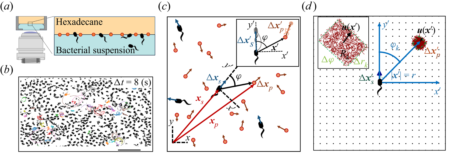
Figure 1. Correlated displacement velocimetry. (a) Schematic of the experimental set-up. Bacteria and passive tracers are observed on a planar hexadecane–water interface. (b) Trajectories of bacteria and tracers over a time interval  $\Delta t = 8\ {\rm s}$: black trajectories indicate tracers; coloured trajectories indicate bacteria; scale bar measures
  $20\ \mathrm {\mu }{\rm m}$. (c) Schematic of the laboratory frame
  $(x,y)$ and common frame
  $(x',y')$ coordinate systems. To measure the flow field from the correlated displacements of tracers and bacteria, a common coordinate system is defined with each swimming bacterium at the origin and the
  $y'$ axis aligned with the swimming direction. Inset: transformed displacement vectors from the laboratory frame to the common frame. (d) To measure the flow field, tracer displacements in the common frames are sampled in a different region
  $R_k$ based on their locations in the common frame. Inset: zoomed-in view of tracer displacements (red vectors) in the region
  $R_k$ with centre location
  $\boldsymbol {r}_k$ and size
  $\Delta r_k$ and
  $\Delta \varphi$; average displacement in each region weighted by the displacements of the swimmers results in the flow field at
  $\boldsymbol {r}_k$.
2.2. Correlated displacement velocimetry
Correlated displacement velocimetry (CDV) was introduced by Molaei et al. (Reference Molaei, Chisholm, Deng, Crocker and Stebe2021) for measuring flow disturbances associated with the Brownian motion of colloidal particles. Here, we describe this technique in detail and adapt it to measure the far-field flow field generated by an actively swimming bacterium. This CDV relies on the fact that bacteria move in an uncorrelated manner in a sufficiently dilute interfacial suspension of swimmers and passive tracer particles. Therefore, we can isolate statistically the approximate flow disturbance due to the locomotion of an individual bacterium by correlating the displacements of each bacterium with the displacements of the surrounding tracer particles over a short time interval or ‘lag time’, and superposing the results. Specifically, we obtain the flow field by calculating the covariance of the displacement between pairs of swimmers and tracers. This process filters out the effects of thermal diffusion of the tracer particles and also filters the effects of swimmer–swimmer and tracer–tracer interactions. Moreover, CDV allows us to employ relatively dense tracer particles and swimmers in comparison to standard particle velocimetry techniques.
Here, we show how the covariance of swimmers and tracer displacements over a short period of time reveals the velocity field induced by the swimmer. Consider swimmers interacting with a field of passive tracer particles. Swimmers and tracers are assumed to be adsorbed on the interface and are therefore restricted to translate on the interfacial plane. The positions of the tracer particle and swimmer are denoted  $\boldsymbol {x}_{p}$ and
  $\boldsymbol {x}_{s}$ (or
  $\boldsymbol {x}_{s}^n$ for the
  $n$th swimmer), respectively; these vectors are measured from an arbitrary origin in the laboratory frame. The displacements of bacteria and tracers are treated as random variables. Their correlated motion is determined by measuring the covariance of their displacements over the observation lag time. During lag time
  $\tau$, the
  $n$th swimmer undergoes displacement
  $\Delta \boldsymbol {x}_{s}^n(\tau )$, and a passive tracer located at position
  $\boldsymbol {x}$ undergoes displacement
  $\Delta \boldsymbol {x}_{p}(\boldsymbol {x}, \tau )$.
Considering first the motion of the tracer particles, the displacement of each passive tracer has contributions from the flow field induced by all swimmers in the system. Tracers also undergo Brownian motion and may interact with one another through electrostatic, capillary or other means. Thus the displacement vector of a given tracer particle centred at position  $\boldsymbol {x}$ over lag time
  $\tau$ interacting with
  $N_{s}$ swimmers and
  $N_{p}-1$ other particles can be expressed as
 \begin{equation} \Delta \boldsymbol{x}_{p}(\boldsymbol{x}, \tau) = \sum_{n=1}^{N_{s}}{\Delta\boldsymbol{x}_{sp}^{n}}(\boldsymbol{x}, \tau) + \Delta\boldsymbol{x}_{p,T}(\boldsymbol{x}, \tau) + \sum_{n=1}^{N_{p} - 1}{\Delta\boldsymbol{x}_{pp}^{n}}(\boldsymbol{x}, \tau), \end{equation}
where  $\Delta \boldsymbol {x}_{sp}^{n}(\boldsymbol {x}, \tau )$ is the displacement of a particle at
  $\boldsymbol {x}$ induced by the flow disturbance of the
  $n$th swimmer,
  $\Delta \boldsymbol {x}_{p,T}$ is the Brownian displacement of the tracer (which has zero mean value), and
  $\Delta \boldsymbol {x}_{pp}^{n}$ represents the displacement due to interactions with the
  $n$th (other) tracer particle.
The displacement of the swimmer during lag time  $\tau$ is given by
  $\Delta \boldsymbol {x}_{s}(\tau ) = \int _0^\tau \boldsymbol {v}_{s}(t) \,\mathrm {d} t$, where
  $\boldsymbol {v}_{s}$ is the swimming velocity. Over short lag times, we can assume that swimming velocity is constant, i.e.
  $\boldsymbol {v}_{s}(t) = \boldsymbol {v}_{s}(0) + O(\tau )$. Thus the displacement of the
  $n$th swimmer is approximated by
 \begin{equation} \Delta\boldsymbol{x}_{s}^n(\tau) = \tau\,\boldsymbol{v}_{s}^n(0), \end{equation}
where we neglect  $O(\tau ^2)$ contributions.
We now introduce a ‘common’ reference frame having Cartesian coordinates  $(x', y')$, which places all bacteria at the origin with swimming direction in the
  $+y'$ direction. In other words, the common frame corresponds to
  $N_{s}$ different ‘views’ of the laboratory frame, each one being co-located and co-aligned with the
  $n$th swimmer. In this frame, we define unit vectors
  $\boldsymbol {e}_{x'}$ and
  $\boldsymbol {e}_{y'}$, which point in the
  $x'$ and
  $y'$ directions, respectively, and we may express the position vector in the common frame as
 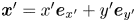 $\boldsymbol {x}' = x' \boldsymbol {e}_{x'} + y' \boldsymbol {e}_{y'}$. Notice that a single point in the common frame maps to
  $n$ points in the laboratory frame as
 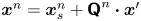 $\boldsymbol {x}^n = \boldsymbol {x}_{s}^n + {\boldsymbol{\mathsf{Q}}}^n \boldsymbol {\cdot } \boldsymbol {x}'$, where
 \begin{equation} {\boldsymbol{\mathsf{Q}}}^n = \boldsymbol{p}^n \boldsymbol{e}_{x'} + \boldsymbol{q}^n \boldsymbol{e}_{y'}. \end{equation}
The orthonormal pair of vectors  $\boldsymbol {p}^n$ and
  $\boldsymbol {q}^n$ appearing in (2.3) are perpendicular and parallel to the swimming direction of the
  $n$th bacterium, respectively. Specifically, we define
  $\boldsymbol {q}^n$ by
  $\boldsymbol {v}_{s}^n = \boldsymbol {q}^n v_{s}^n$, where
  $v_{s}^n = \left \lVert \boldsymbol {v}_{s}^n\right \rVert$ is the swimming speed of the
  $n$th bacterium.
The covariance of the magnitude of the swimmer displacements and the displacement of a tracer particle located at a fixed position  $\boldsymbol {x}'$ in the common frame is given by
 \begin{equation} \boldsymbol{\chi}(\boldsymbol{x}', \tau) = \left\langle \left\lVert\Delta \boldsymbol{x}_{s}^n(\tau)\right\rVert {\boldsymbol{\mathsf{Q}}}^{\prime n} \boldsymbol{\cdot} {\Delta \boldsymbol{x}_{p}}(\boldsymbol{x}^n_{s} + {\boldsymbol{\mathsf{Q}}}^n \boldsymbol{\cdot} \boldsymbol{x}', \tau) \right\rangle_n, \end{equation}
where  ${\boldsymbol{\mathsf{Q}}}^{\prime n}$ is the transpose of
  ${\boldsymbol{\mathsf{Q}}}^n$, and
  $\left \langle \,{\cdot}\, \right \rangle _n$ denotes the expected value of the ensemble over all swimmers. Considering the different contributions to
  $\Delta \boldsymbol {x}_{p}$ expressed by (2.1) and using (2.2), we may rewrite (2.4) as
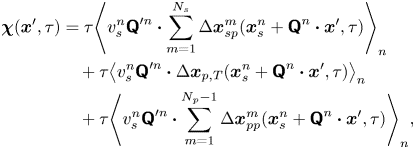 \begin{align} \boldsymbol{\chi}(\boldsymbol{x}', \tau) &= \tau{\left\langle v_{s}^n {\boldsymbol{\mathsf{Q}}}^{\prime n} \boldsymbol{\cdot} \sum_{m=1}^{N_{s}} \Delta \boldsymbol{x}_{sp}^m(\boldsymbol{x}^n_{s} + {\boldsymbol{\mathsf{Q}}}^n \boldsymbol{\cdot} \boldsymbol{x}', \tau) \right\rangle}_n \nonumber\\ &\quad + \tau{\left\langle v_{s}^n {\boldsymbol{\mathsf{Q}}}^{\prime n} \boldsymbol{\cdot} \Delta\boldsymbol{x}_{p,T}(\boldsymbol{x}^n_{s} + {\boldsymbol{\mathsf{Q}}}^n \boldsymbol{\cdot} \boldsymbol{x}', \tau) \right\rangle}_{n} \nonumber\\ &\quad + \tau{\left\langle v_{s}^n {\boldsymbol{\mathsf{Q}}}^{\prime n} \boldsymbol{\cdot} \sum_{m=1}^{N_{p} - 1} \Delta\boldsymbol{x}_{pp}^{m}(\boldsymbol{x}^n_{s} + {\boldsymbol{\mathsf{Q}}}^n \boldsymbol{\cdot} \boldsymbol{x}', \tau) \right\rangle}_n, \end{align}
where we note that the product  $v_{s}^n {\boldsymbol{\mathsf{Q}}}^{\prime n}$ depends only on the swimming velocity of the
  $n$th bacterium (
 ${\boldsymbol{\mathsf{Q}}}^{\prime n}$ encodes swimming direction). Regarding the first term of (2.5), we may assume that the bacterial concentration is sufficiently dilute that the swimming velocities of different bacteria are uncorrelated. Then all terms in the summation under the average are negligibly small except for when
  $n = m$. Furthermore, the second and third terms of (2.5) can be neglected entirely. The second term is negligible because the effect of Brownian motion on the velocity of a bacterium is generally much smaller than contributions due to active swimming. Therefore, the swimmer's displacement and the tracers’ Brownian displacement are correlated only weakly. The third term vanishes because the particle displacements due to sources other than flow disturbances produced by the bacteria are uncorrelated with the swimming velocities of the bacteria. Moreover, the displacement of a bacterium due to interactions with tracer particles is small compared to the displacements due to active swimming. Therefore, while
  $\Delta \boldsymbol {x}_{pp}$ is not necessarily small, its correlation with the swimmer velocity is negligible. With these simplifications, (2.5) reduces to
 \begin{equation}
\boldsymbol{\chi}(\boldsymbol{x}', \tau) = \tau\langle
v_{s}^n \, {\boldsymbol{\mathsf{Q}}}^{\prime n} \boldsymbol{\cdot}
\Delta \boldsymbol{x}_{sp}^n(\boldsymbol{x}_{s}^n +
{\boldsymbol{\mathsf{Q}}}^n \boldsymbol{\cdot} \boldsymbol{x}', \tau) \rangle_n. \end{equation}
\begin{equation}
\boldsymbol{\chi}(\boldsymbol{x}', \tau) = \tau\langle
v_{s}^n \, {\boldsymbol{\mathsf{Q}}}^{\prime n} \boldsymbol{\cdot}
\Delta \boldsymbol{x}_{sp}^n(\boldsymbol{x}_{s}^n +
{\boldsymbol{\mathsf{Q}}}^n \boldsymbol{\cdot} \boldsymbol{x}', \tau) \rangle_n. \end{equation}
Recall that  $\Delta \boldsymbol {x}_{sp}^{n}(\boldsymbol {x}, \tau )$ describes the displacements of particles in the laboratory frame induced by the flow disturbance induced by the
  $n$th swimmer. Let
  $\boldsymbol {u}^n(\boldsymbol {x})$ denote this flow disturbance. Assuming that the tracer particles are sufficiently small, their displacement due to this flow disturbance at small lag times is given by
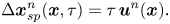 \begin{equation} \Delta \boldsymbol{x}^n_{sp}(\boldsymbol{x}, \tau) = \tau\,\boldsymbol{u}^n(\boldsymbol{x}). \end{equation}
In terms of a fixed position  $\boldsymbol {x}'$ in the common frame, we may express the velocity disturbance produced by the
  $n$th bacterium as
 \begin{equation} \boldsymbol{u}^n(\boldsymbol{x}_{s}^n + {\boldsymbol{\mathsf{Q}}}^n \boldsymbol{\cdot} \boldsymbol{x}') = {\boldsymbol{\mathsf{Q}}}^n \boldsymbol{\cdot} \boldsymbol{u}^{\prime n}(\boldsymbol{x}'). \end{equation}
Then, using (2.7) and (2.8) in (2.6) yields
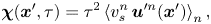 \begin{equation} \boldsymbol{\chi}(\boldsymbol{x}', \tau) = \tau^2 \left\langle v_{s}^n\,\boldsymbol{u}^{\prime n}(\boldsymbol{x}') \right\rangle_n, \end{equation}
where we have used the identity  ${\boldsymbol{\mathsf{Q}}}^{\prime n} \boldsymbol {\cdot } {\boldsymbol{\mathsf{Q}}}^{n} = {\boldsymbol{\mathsf{I}}}$, where
  ${\boldsymbol{\mathsf{I}}}$ is the identity tensor.
We now assume that the interface is homogeneous in its mechanics so that the velocity fields produced by the bacteria are spatially invariant. Then we may write  $\boldsymbol {u}^{\prime n}$ as the sum
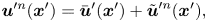 \begin{equation} \boldsymbol{u}^{\prime n}(\boldsymbol{x}') = \bar{\boldsymbol{u}}'(\boldsymbol{x}') + \tilde{\boldsymbol{u}}^{\prime n}(\boldsymbol{x}'), \end{equation}
where  $\bar {\boldsymbol {u}}' = \left \langle \boldsymbol {u}^{\prime n} \right \rangle _n$ is the mean velocity disturbance that, in the laboratory frame, differs from bacterium to bacterium only due to differences in their swimming directions or position. On the other hand,
  $\tilde {\boldsymbol {u}}^n$ represents the difference of the
  $n$th bacterium from this mean due to variations in everything other than position and direction: swimming speed, bacterium geometry, trapped state, etc. Thus we may interpret
  $\bar {\boldsymbol {u}}'$ as the velocity disturbance produced by an ‘average’ bacterium.
Using (2.8) and (2.10) in (2.9), we obtain for the swimmer–tracer displacement covariance
 \begin{equation} \boldsymbol{\chi}(\boldsymbol{x}', \tau) = \tau^2 \bar{v}_{s}\,\bar{\boldsymbol{u}}'(\boldsymbol{x}') + \tau^2 \left\langle v_{s}^n\, \tilde{\boldsymbol{u}}^{\prime n}(\boldsymbol{x}') \right\rangle_n, \end{equation}
where  $\bar {v}_{s} = \left \langle v_{s}^n \right \rangle _n = \tau ^{-1} \left \langle \sqrt {\Delta \boldsymbol {x}_{s}^n \boldsymbol {\cdot } \Delta \boldsymbol {x}_{s}^n} \,\right \rangle _n$ is the average swimming speed. The second term in (2.11) can be eliminated under the assumption that swimming velocity and the corresponding flow disturbance due to a swimmer are related linearly. This assumption is reasonable given that bacteria swim at very small Reynolds numbers. Thus letting
  $\tilde {\boldsymbol {u}}^{\prime n} = v_{s}^n \tilde {\boldsymbol {w}}^{\prime n}$, where
  $\tilde {\boldsymbol {w}}^{\prime n}$ is dimensionless and independent of
  $v_{s}^n$, the second term in (2.11) reduces to
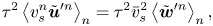 \begin{equation} \tau^2 \left\langle v_{s}^n \tilde{\boldsymbol{u}}^{\prime n} \right\rangle_n = \tau^2 \bar {v}_{s}^2 \left\langle \tilde{\boldsymbol{w}}^{\prime n} \right\rangle_n, \end{equation}
which vanishes because 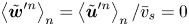 $\left \langle \tilde {\boldsymbol {w}}^{\prime n} \right \rangle _n = \left \langle \tilde {\boldsymbol {u}}^{\prime n} \right \rangle _n / \bar {v}_{s} = 0$. With this term eliminated, solving (2.11) for
  $\bar {\boldsymbol {u}}'$ yields the mean velocity disturbance as
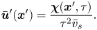 \begin{equation} \bar{\boldsymbol{u}}'(\boldsymbol{x}') = \frac{\boldsymbol{\chi}(\boldsymbol{x}', \tau)}{\tau^2 \bar{v}_{s}}. \end{equation}
2.3. Experimental implementation of CDV
To use (2.13) for computing the mean bacterium-induced velocity disturbance  $\bar {\boldsymbol {u}}'$, we must compute
  $\boldsymbol {\chi }$ from experimental swimmer and tracer displacement data. We therefore evaluate particle and swimmer displacements over lag time
  $\tau$ at various positions
  $\boldsymbol {x}'$ around the swimmer directly in the common frame, as illustrated in figure 1(d). As we cannot compute the true expected value represented by
  $\boldsymbol {\chi }$, we must instead approximate
  $\boldsymbol {\chi }$ using a sufficiently large sample size and implement a method to control sampling error. In particular, the number of swimmer–tracer displacement products considered at each position must be large enough for the signal to emerge from Gaussian noise. Here, our strategy is to discretize the spatial domain and to bin appropriately displacement products.
Given the form of the flow field, which decays with distance from each swimmer, it is advantageous to construct these bins using a polar coordinate system in the common frame, adjusting bin size with distance from the swimmer. Here, the common frame acts as a ‘sampling space’ where we can bin together related displacement data over multiple observations of multiple bacteria, all providing independent realizations of the ensemble. This grid is parametrized by  $\boldsymbol {x}' = -\boldsymbol {e}_{x'} r \sin \varphi + \boldsymbol {e}_{y'} r\cos \varphi$, where
  $r = \left \lVert \boldsymbol {x}'\right \rVert$ and
  $\varphi$ is the angle measured CCW from the
  $y'$ axis. We then consider a set of bins arranged on this grid, where the
  $k$th bin spans the region
  $R_k$ given by
  $r_k - \Delta r_k / 2 < r < r_k + \Delta r_k / 2$ and
  $\varphi _k - \Delta \varphi / 2 < \varphi < \varphi _k + \Delta \varphi / 2$. We choose
  $\Delta \varphi$ to be the fixed value
  ${\rm \pi} /60$, and
  $\Delta r$ to increase in proportion with
  $r^3$. With this discretization scheme, the number of particle displacement vectors in each bin scales as
  $\Delta \varphi \,r\,\Delta r \sim r^4$, ensuring a constant signal-to-noise ratio across the field of the measurement. We now consider the computation of
  $\boldsymbol {\chi }$ in each bin. In the laboratory frame, the
  $n$th swimmer undergoes displacement
  $\Delta \boldsymbol {x}_{s}^n$, and the
  $m$th passive tracer undergoes displacement
  $\Delta \boldsymbol {x}_{p}^m$ over lag time
  $\tau$ (figure 1c). In the common frame, as applied to the position and orientation of the
  $n$th bacterium, that same swimmer undergoes displacement
  $\Delta \boldsymbol {x}^{\prime n}_{s}$ in the
  $+y'$ direction, and the passive tracer undergoes displacement
  $\Delta \boldsymbol {x}^{\prime m}_{p}$. The laboratory-frame and common-frame swimmer and particle displacements are related by
  $\Delta \boldsymbol {x}_{s}^{\prime n} = \boldsymbol {e}_{y'} \left \lVert \Delta \boldsymbol {x}_{s}^n\right \rVert$ and
  $\Delta \boldsymbol {x}_{p}^{\prime m} = {\boldsymbol{\mathsf{Q}}}^{\prime n} \boldsymbol {\cdot } {\Delta \boldsymbol {x}_{p}^{\prime m}}$, respectively. Each active swimmer displacement vector
  $\Delta \boldsymbol {x}_{s}^{\prime n}$ is considered as a source that generates correlated displacements of tracer particles in the domain. We then approximate
  $\boldsymbol {\chi }(\boldsymbol {x}', \tau )$ for
  $\boldsymbol {x}'$ in the
  $k$th bin as
 \begin{equation} \boldsymbol{\chi}(\boldsymbol{x}' \in R_k, \tau) \approx \boldsymbol{\chi}^k = \langle \left\lVert\Delta \boldsymbol{x}_{s}^n\right\rVert \Delta \boldsymbol{x}_{p}^{\prime m} \rangle^k_{m,n}, \end{equation}
where we use the notation  $\left \langle \,{\cdot}\, \right \rangle ^k_{m,n}$ to denote the sample mean over all
  $n = 1, \ldots, N_{s}$ bacteria and the subset of tracer particles located in
  $k$th bin (
 $\boldsymbol {x}_{p}^{\prime m} \in R_k$) before displacing by
  $\Delta \boldsymbol {x}_{p}^{\prime m}$. Thus we regard the particle index
  $m$ in the average in (2.14) as running over
 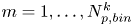 $m = 1, \ldots, N^k_{{p,bin}}$, where
  $N^k_{{p,bin}}$ is the number of tracer particles in the
  $k$th bin. The mean velocity disturbance due to a bacterium is then evaluated from (2.13) as
 \begin{equation} \bar{\boldsymbol{u}}^{\prime k} \approx \frac{\boldsymbol{\chi}^k}{\tau^2 \bar{v}_{s}} \end{equation}
for points lying in the  $k$th bin.
The number of particle displacement vectors in each bin must be large enough to ensure that  $\boldsymbol {\chi }^k$ is a good approximation to
  $\boldsymbol {\chi }$ for
  $\boldsymbol {x}' \in R_k$. This task is most difficult for points in the far field of the reported displacement field (
 $r > 60\ \mathrm {\mu }{\rm m}$), where displacements are weakest. Therefore, we require
  $N_{{p,bin}}^k \ge N_{p,min}$, where
  $N_{p,min}$ is the minimum number of tracer particles necessary to resolve small hydrodynamic displacements
  $\boldsymbol {u}(\boldsymbol {r})\,\tau$ in the presence of noise from random Brownian motion. The measurement error in evaluating (2.13) owing to Brownian noise in the
  $k$th bin is proportional to
 \begin{equation} \sqrt{\langle \Delta \boldsymbol{x}_{p}^m(\tau)^2\rangle_{N_p}}\Big/{2\tau \sqrt{N^k_{p, bin}}}. \end{equation}
In this study, we require  $N_{p,min}=10^6$ in the far field. Thus the measurement error is orders of magnitude smaller than hydrodynamic displacements of
  ${\sim }1\ {\rm nm}$ for particles undergoing Brownian displacements of
  ${\sim }100\ {\rm nm}$ over
  $\tau = 0.2\ {\rm s}$.
3. Physico-chemistry of the fluid interface
We study bacteria swimming at the aqueous–hexadecane interface with characteristic velocity  $v= 10\ \mathrm {\mu }{\rm m}\ {\rm s}^{-1}$ and characteristic cell body size
  $a= 1\ \mathrm {\mu }{\rm m}$. The average viscosity of the bulk aqueous and oil phases is
  $\bar \mu = 2.17\times 10^{-3}\ {\rm Pa}\ {\rm s}$. The bacteria swim with negligible Reynolds number
  $Re = \rho v a / \bar {\mu } \approx 10^{-4}$, where
  $\rho$ is the density of water. Therefore, the fluids above and below the interface can be assumed to be in the creeping flow regime. An independent upper bound of the surface viscosity can be determined in situ using the same CDV techniques that we use to determine the flow field around the swimming bacteria (Molaei et al. Reference Molaei, Chisholm, Deng, Crocker and Stebe2021). By analysing the correlated motion of tracer–tracer pairs (rather than swimmer–tracer pairs as in § 2.2) via CDV, we find bounding values for the surface viscosity
  $\mu _s = 1.5\times 10^{-9}\ {\rm Pa}\ {\rm s}\ {\rm m}$ and Boussinesq number
  $Bo = l_s/a < 0.7$, where
  $l_s = \mu _s / \bar \mu$. We also measure the equilibrium surface tension
  $\sigma _{eq}$ of the hexadecane–buffer interface, which we find is
  $\sigma _{eq} \approx 46.7\ {\rm mN}\ {\rm m}^{-1}$. This value is less than the expected surface tension
  $55.2\ {\rm mN}\ {\rm m}^{-1}$ (Goebel & Lunkenheimer Reference Goebel and Lunkenheimer1997). The difference indicates the presence of adsorbed surfactant, likely from impurities in the oil, impurities in the buffer, or bacterial secretions.
The flow from the swimming bacterium can redistribute surfactant, generating a surface pressure gradient or Marangoni stress that opposes bacteria motion. We define the surface pressure as  $\varPi = \sigma _{eq} - \sigma$, where
  $\sigma$ is the (dynamic) surface tension. The relative importance of the Marangoni stress to the viscous stress is captured by the Marangoni number
 \begin{equation} Ma = \frac{\bar{\varGamma}}{\bar{\mu} v}\,\frac{\partial\varPi}{\partial\varGamma}, \end{equation}
where  $\bar {\varGamma }$ is the average surface concentration of surfactant. In the limit of extremely low surfactant concentrations (e.g.
  $\bar {\varGamma }= 10^{3}\,{\rm molecules}\ \mathrm {\mu }{\rm m}^{-2}$), the interface exhibits a gaseous state with
 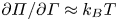 ${\partial \varPi }/{\partial \varGamma }\approx k_B T$. Even in this very dilute regime, Marangoni stresses are remarkably significant; we find from (3.1) that
  $Ma \approx 150$. Furthermore, for dilute surfactants, mass fluxes between the interface and the bulk are negligible. The distribution of surfactants is determined by surface advection, as influenced by fluid flow disturbances produced by the bacteria, Marangoni flows and surface diffusion. Thus the mass balance of the surfactant is given by
 \begin{equation} \boldsymbol{\nabla}_s \boldsymbol{\cdot} (\boldsymbol{v}\varGamma) - D_s\,\boldsymbol{\nabla}_s^2 \varGamma= 0, \end{equation}
where  $D_s$ is the surface diffusivity of the surfactant, and
  $\boldsymbol {v}$ is the fluid velocity field at the interface. The relative importance of surface advection versus surface diffusion is characterized by the product of the Marangoni and Péclet numbers
  $Ma\,Pe$, where the Péclet number is
  $Pe = a v / D_s$. For typical values of
  $D_s$, approximately
  $10\ \mathrm {\mu }{\rm m}^2\ {\rm s}^{-1}$, we estimate
  $Pe\sim 1$. Then, in the limit of large
  $Ma$,
$Ma$,  $Ma\,Pe$ is also large. In this case, viscous stress generated by the swimmer cannot compress the surfactant monolayer appreciably, and the interface must be treated as an incompressible two-dimensional layer (Bławzdziewicz et al. Reference Bławzdziewicz, Cristini and Loewenberg1999; Fischer et al. Reference Fischer, Dhar and Heinig2006; Chisholm & Stebe Reference Chisholm and Stebe2021). Similar to the manner in which the hydrodynamic pressure enforces fluid incompressibility in a bulk fluid, the surface pressure gradient in the interface enforces the interfacial incompressibility constraint.
4. Characterization of the trapped state of bacteria at the interface
The cell bodies of the bacteria are trapped at the interface in a variety of configurations. These configurations will affect the flow disturbance generated by each bacterium. We estimate the configurations of the cell bodies using data accessible in our experiment. While we do not have a side view of the cell bodies, we do record the projected image (or silhouette) of each cell body on the interfacial plane. The cell bodies of P. aeruginosa may be approximated as a spherocylinder, i.e. a right circular cylinder with hemispherical end caps of the same radius (de Anda et al. Reference de Anda2017). The aspect ratio of each cell body,  $\gamma$, is calculated from the measurement of the cell body length
  $l$ over width
  $w$ at the interface. Weak fluctuations in
  $\gamma$ for each cell indicate that cell bodies do not change their configuration with time; this indicates that cells likely adsorb onto the interface with pinned contact lines (see figure S3 of the supplementary material). Qualitatively, more elongated cell body aspect ratios are associated with trapped configurations that are aligned more parallel to the interface.
Since our experimental apparatus requires a long working distance imaging system, the numerical aperture (NA) of the objective is small, leading to low diffraction limited resolution. A conservative estimate of the uncertainty in the apparent size of the bacteria due to the diffraction limited resolution is  $\delta l \approx \lambda _w/4\,\text {NA} \approx 0.25\ \mathrm {\mu }{\rm m}$, where
  $\lambda _w$ is the centre wavelength of the visible spectrum. This limited resolution creates uncertainty in the apparent aspect ratio.
Bacteria vary in aspect ratio. To characterize this natural dispersion, we use high resolution bright field images of PA01 fixed on agar plates (see figure S4 of the supplementary material) to obtain probability distributions of the cell body widths  $w_b$, lengths
  $l_b$ and aspect ratios
  $\gamma _b$ (see figures S5 and S6 of the supplementary material). While cell body lengths vary significantly as bacteria grow in length prior to cell division, their widths vary comparatively weakly, with median value
  $0.70\ \mathrm {\mu }{\rm m}$. For comparison, the probability distributions of the cell body widths, lengths and aspect ratios at the interface are also calculated (see figures S5 and S7 of the supplementary material). The mean value for the cell body width observed at the interface is
  $0.93\ \mathrm {\mu }{\rm m}$. This apparent mean width is greater than that of the well-resolved cell body owing to the limitations of our optics, and is an indication of systematic error. The resulting uncertainty in the apparent aspect ratio can be estimated as
  $\delta \gamma \approx \sqrt {1+\gamma ^2}\,\delta l/w_b$.
The natural dispersion of cell body aspect ratios requires care in estimating the trapping angle  $\theta$ from the observed
  $\gamma$. We use the probability distribution of
  $\gamma _b$ and
  $\gamma$ to find a function that maps the observed
  $\gamma$ to the trapping angle via Bayesian inference, noting that if
  $\gamma$ is observed, then the probability is
  $P(\gamma _b<\gamma )=0$. The mapping is reported in figure S1. The details of this calculation are provided in the supplementary material available at https://doi.org/10.1017/jfm.2023.905. We emphasize that this estimated trapping angle is uncertain owing to the large uncertainty in the apparent aspect ratio of the cell body at the interface.
5. Hydrodynamics of interfacially trapped bacteria
Figure 2(d) depicts the measured, ensemble-averaged flow field generated by the population of bacteria at the interface swimming in pusher mode. The flow field is dominated by bacteria with speed, trajectory curvature and apparent trapping angle near the median values of these properties ( $\bar {v}_{s} = 9.8\ \mathrm {\mu }{\rm m}\ {\rm s}^{-1}$,
  $\bar {\kappa } = 0.2\ \mathrm {\mu }{\rm m}^{-1}$,
  $\bar {\theta } = 46^{\circ }$). While this flow field decays as
  $1/r^{2}$ in all directions (figure 2b), its structure differs significantly from the fore–aft symmetric bulk stresslet generated by a pusher in the bulk (Lauga Reference Lauga2016). Rather, the observed flow field has broken fore–aft symmetries and distinct closed streamlines. The observed flow also differs significantly from the flow field reported for pushers near solid surfaces (Drescher et al. Reference Drescher, Dunkel, Cisneros, Ganguly and Goldstein2011). These differences are particularly notable since a viscosity-averaged stresslet with functional form like the bulk stresslet is a solution for Stokes flow in an interface characterized solely by a uniform interfacial tension (Chisholm & Stebe Reference Chisholm and Stebe2021).

Figure 2. Interfacial flow around a pusher bacterium. (a) Schematic of an adsorbed bacterium and passive tracer particles that moves in the interface with propulsive force  $\boldsymbol {F}_P$ that is resisted by drag force
  $\boldsymbol {F}_D$. (b) Plots of the spatial decay of the velocity field
  $\boldsymbol {u}(\boldsymbol {r})$ along the
  $x'$ and
  $y'$ axes. (c) Plots of the theoretical fit of the bacterial flow field. (d) Plots of the measured flow field generated by an ensemble of bacteria. Streamlines indicate the local direction of the flow, and the heat map indicates flow speed. (e,f) Plots of the
  ${\boldsymbol{\mathsf{S}}}$ mode and
  $\boldsymbol {B}$ mode components of the theoretical fit in (c), respectively. These modes are superposed, with the singular point of both modes shifted to position
  $y' = \delta y$, and have tilt angles
  $\phi ^S$ and
  $\phi ^B$, respectively.
To understand the flow structure, we consider the manner in which interfacial trapping alters swimmer hydrodynamics. We assume that interfacially trapped bacteria have flagella rotating in the aqueous sub-phase (figure 2a) that generate the propulsion force that drives their motion. While the opposite arrangement, where the flagellum protrudes into the oil phase, is also possible, this arrangement likely leads to an immotile bacterium, because the molecular motor that drives the flagellum requires a flux of cations including hydrogen and sodium in order to function (Nakamura & Minamino Reference Nakamura and Minamino2019). The transport of such ions into the oil phase is hindered by water's superior solvation capacity (Wu, Iedema & Cowin Reference Wu, Iedema and Cowin1999). The rotation of the flagellum also generates a reactionary torque that favours rotation of the cell body along an axis lying in the plane of the interface. However, such rotational motion is prevented by contact-line pinning. Recall that our measurements of cell body configuration and the persistence of bacterial swimming mode suggest that such contact-line pinning is a likely scenario (Deng et al. Reference Deng, Molaei, Chisholm and Stebe2020). Translation perpendicular to the interface is also precluded by contact-line pinning and by the interfacial tension  $\sigma$, which is large compared to any viscous stresses generated by the swimmer, as described by the capillary number
  $Ca=\bar {\mu }v/\sigma \approx 10^{-6}$. Furthermore, the stress state of fluid interfaces is complex, with Marangoni stresses due to surface tension gradients that oppose the swimmer motion, and surface viscosities that generate dissipation.
Hydrodynamic theory for a swimmer trapped on an incompressible interface suggests that the flow sufficiently far from the bacterium is dominated by a superposition of two flow modes, which we call the ‘ ${\boldsymbol{\mathsf{S}}}$’ and ‘
 $\boldsymbol {B}$’ modes (Chisholm & Stebe Reference Chisholm and Stebe2021). These modes are associated with different components of the first moment of the stress exerted by the moving bacterium surface on the surrounding fluid and on the interface. Formally, they are the dipolar terms in a multipole expansion of the velocity field about about an appropriate point in the immediate vicinity of the bacterium, which we call the ‘hydrodynamic origin’, denoted
  $\boldsymbol {x}'_h = \langle x'_h, y'_h \rangle$. The
  ${\boldsymbol{\mathsf{S}}}$ mode arises from the projection of these stresses onto the interfacial plane and is thus termed an ‘interfacial stresslet’; it is analogous to the stresslet generated by Stokesian swimmers in a bulk fluid (Lauga & Powers Reference Lauga and Powers2009). The corresponding flow field is shown in figure 2(e). The
  $\boldsymbol {B}$ mode, on the other hand, is associated with the protrusion of the bacterium's body and flagellum into the fluid phases. Finite ‘vertical’ separation from the interfacial plane of viscous stresses along the bacterium surface gives rise to a finite tangential stress jump across the interface. This stress discontinuity is supported by the gradients in surface tension that enforce the incompressibility constraint. The flow field generated by the
  $\boldsymbol {B}$ mode, shown in figure 2(f), corresponds to the two-dimensional potential flow due to a source–sink doublet. The superposition of these modes leads to the fore–aft asymmetric flow in figure 2(d).
The analytical form of the flow field generated by the  ${\boldsymbol{\mathsf{S}}}$ mode on the interfacial plane is given by
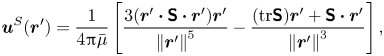 \begin{equation} \boldsymbol{u}^S(\boldsymbol{r}') = \frac{1}{4{\rm \pi}\bar\mu} \left[ \frac{3 (\boldsymbol{r}' \boldsymbol{\cdot} {\boldsymbol{\mathsf{S}}} \boldsymbol{\cdot} \boldsymbol{r}')\boldsymbol{r}'}{\left\lVert\boldsymbol{r}'\right\rVert^5} - \frac{(\textrm{tr}{{\boldsymbol{\mathsf{S}}}}) \boldsymbol{r}' + {\boldsymbol{\mathsf{S}}} \boldsymbol{\cdot} \boldsymbol{r}'}{\left\lVert\boldsymbol{r}'\right\rVert^3} \right], \end{equation}
where  ${\boldsymbol{\mathsf{S}}}$ is a second-order tensor whose components have units of force times length, and
  $\boldsymbol {r}' = \boldsymbol {x}' - \boldsymbol {x}'_h$ is the position vector relative to the hydrodynamic origin
  $\boldsymbol {x}'_h$. The tensor
  ${\boldsymbol{\mathsf{S}}}$, which is denoted
  ${\boldsymbol{\mathsf{S}}}^{\,\shortparallel }$ in Chisholm & Stebe (Reference Chisholm and Stebe2021), has the property of being traceless and symmetric, i.e.
  $\textrm {tr}\,{{\boldsymbol{\mathsf{S}}}} = 0$ and
  ${\boldsymbol{\mathsf{S}}} = {\boldsymbol{\mathsf{S}}}^{\rm T}$, respectively, where
  $^{\rm T}$ denotes the transpose. Therefore,
  ${\boldsymbol{\mathsf{S}}}$ has two eigenvalues,
  $+\lambda ^S$ and
  $-\lambda ^S$, associated with a pair of orthonormal eigenvectors. The eigenvector
  $\boldsymbol {q}^S$ associated with the positive eigenvalue is aligned with the axis of an interfacial extensional flow produced by the bacterium, and defines a natural ‘direction’ of the
  ${\boldsymbol{\mathsf{S}}}$ mode. We therefore introduce the
  ${\boldsymbol{\mathsf{S}}}$ mode orientation angle
  $\phi ^S$ as the angle of
  $\boldsymbol {q}^S$ relative to the vertical axis, i.e.
 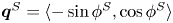 $\boldsymbol {q}^S = \langle -\sin \phi ^S, \cos \phi ^S \rangle$. The
  ${\boldsymbol{\mathsf{S}}}$ mode can also be associated with a scalar strength
  $S = 2\lambda ^S$. For a perfect dipole consisting of two opposite point forces of strength
  $F$ separated by a distance
  $l$ parallel to the interfacial plane, the
  ${\boldsymbol{\mathsf{S}}}$ mode strength is
  $S = Fl$ (see the supplementary material for details).
The flow field generated by the  $\boldsymbol {B}$ mode is given by
 \begin{equation} \boldsymbol{u}^B(\boldsymbol{r}') =\frac{1}{8{\rm \pi}\bar\mu}\left[\frac{\boldsymbol{B}}{\left\lVert\boldsymbol{r}'\right\rVert^2} - \frac{2 (\boldsymbol{B} \boldsymbol{\cdot} \boldsymbol{r}') \boldsymbol{r}'}{\left\lVert\boldsymbol{r}'\right\rVert^4} \right] = \frac{B}{8{\rm \pi}\bar\mu}\left[\frac{\boldsymbol{q}^B}{\left\lVert\boldsymbol{r}'\right\rVert^2} - \frac{2 (\boldsymbol{q}^B \boldsymbol{\cdot} \boldsymbol{r}') \boldsymbol{r}'}{\left\lVert\boldsymbol{r}'\right\rVert^4} \right], \end{equation}
where  $\boldsymbol {B} = B \boldsymbol {q}^B$ is the vector-valued strength of the
  $\boldsymbol {B}$ mode, which has magnitude
  $B = \left \lVert \boldsymbol {B}\right \rVert$ and direction
  $\boldsymbol {q}^B$. Similar to the definition of
  $\boldsymbol {\phi }^S$, we define the
  $\boldsymbol {B}$ mode orientation angle
  $\phi ^B$ based on the unit vector
  $\boldsymbol {q}^B$. We refer the reader to Chisholm & Stebe (Reference Chisholm and Stebe2021) for a detailed derivation and additional discussion of the flow modes given by (5.1) and (5.2).
To compare experiment to theory, the strengths, hydrodynamic origin and directions of the  ${\boldsymbol{\mathsf{S}}}$ and
  $\boldsymbol {B}$ modes are fitted to the observed flow field. Recall that the theoretical derivation of these modes requires that the
  ${\boldsymbol{\mathsf{S}}}$ and
  $\boldsymbol {B}$ modes share the same (hydrodynamic) origin. Thus to reconcile with the theory, we use the same location
  $\boldsymbol {x}'_h$ for both modes, though their orientations differ due to the complex distribution of forces around the cell body. We place the origin of the two dipolar modes along the symmetry axis on the bacterium's body (
 $x_h=0$), and weight these two modes to capture the main features of the observed flow field as shown in figure 2(c). The vector field of each mode is shifted vertically by
  $y'_h$ and rotated CCW by
  $\phi ^S$ and
  $\phi ^B$ to acquire the transformed vector field
  $\boldsymbol {u}'^S$ and
  $\boldsymbol {u}'^B$. The two-dimensional measured velocity field
  $\bar {\boldsymbol {u}}(\boldsymbol {x'})$ is fitted to
  $\boldsymbol {u}'=\boldsymbol {u}'^S +\boldsymbol {u}'^B$ using nonlinear least squares fitting to obtain the dipolar strengths
  $(S, B)$, hydrodynamic origin
  $\boldsymbol {x}_h = \langle 0, y'_h\rangle$ (located along the swimmer's axis of symmetry), and dipole orientations
  $(\phi ^S,\phi ^B)$.
The interfacial stresslet strength 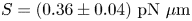 $S = (0.36\pm 0.04)\ {\rm pN}\ \mathrm {\mu }{\rm m}$ is consistent with prior measurements for pusher bacteria in the bulk, and can be estimated as
  $S \approx F_D l$, with
 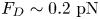 $F_D \sim 0.2\ {\rm pN}$ and
  $l \sim 2\ \mathrm {\mu }{\rm m}$, where
  $F_D$ is the drag force acting on the bacterium, and
  $l$ is the separation distance between two forces on the interfacial plane (Drescher et al. Reference Drescher, Dunkel, Cisneros, Ganguly and Goldstein2011). The direction of the
  ${\boldsymbol{\mathsf{S}}}$ mode is rotated by
  $\phi ^S =( -8.0\pm 2.3)^{\circ }$. The
  $\boldsymbol {B}$ mode has strength
  $B = ({0.82\pm 0.02})\ {\rm pN}\ \mathrm {\mu }{\rm m}$ and is rotated by
  $\phi ^B = ({192.7\pm 4.0})^{\circ }$ with respect to the swimming direction. The expected strength is
  $B\approx F_D h$, where
  $h$ is the distance between the location of the net thrust force and the interfacial plane. Thus the strength of the
  $\boldsymbol {B}$ mode is expected to be of the same order of magnitude as dipolar strength of the stresslet, in keeping with experiment. The origin of the flow field reported in figure 2(d) corresponds to the centre of the cell body; in this coordinate system, the origin of both
  ${\boldsymbol{\mathsf{S}}}$ and
  $\boldsymbol {B}$ modes is located slightly behind the body's centre, displaced by
  $\delta y = (1.33\pm 0.14)\ \mathrm {\mu }{\rm m}$. This placement might be attributed to the elongated shape of the flagellum.
To analyse further the dependence of the flow field generated by bacteria on their trapped configuration, we group the trajectories of swimmers with similar apparent trapping angles according to the mapping in figure S1 and measure the corresponding flow field. For the two flow fields shown in figures 3(a,b), the trapping angle increases from left to right. The bacteria in the more parallel configuration generate a flow field with a more asymmetric shape. The relative strengths of the  ${\boldsymbol{\mathsf{S}}}$ and
  $\boldsymbol {B}$ modes change systematically with the trapping angle (figure 3c). The strength of the
  ${\boldsymbol{\mathsf{S}}}$ mode is largest for parallel swimmers; thus the flow fields of swimmers with small trapping angles have the most pronounced loop-like structures, strong outward flow before the swimmer, and weaker inward flow behind the swimmers, as the strong
  ${\boldsymbol{\mathsf{S}}}$ mode diminishes the inward flow driven by the
  $\boldsymbol {B}$ mode. The strong dependence of the stresslet strength on trapping angle can be rationalized, noting that both
  $F_D$ and
  $l$ are proportional to
  $\cos \theta$ so
 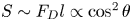 $S\sim F_D l\propto \cos ^2 \theta$. However, the strength of the
  $\boldsymbol {B}$ mode remains approximately fixed. Theory suggests that this mode has a complex dependence on the orientation and position of the thrust force, becoming weaker for forces oriented perpendicular to the interface, and stronger for larger forcing distance from the interface. These two effects give a weak dependence on trapping angle. The
  ${\boldsymbol{\mathsf{S}}}$ and
  $\boldsymbol {B}$ modes are two of the dipolar modes of the stress distribution on a sphere wrapping the bacterium. Their complex dependence on trapping angle suggests that the distribution of thrust forces for bacteria with cell bodies trapped at interfaces is more complex than can be captured by a simple model of two point forces. This inability to predict this observation from this simple model may be attributed to the complex distribution of forces along the surfaces of swimmers’ bodies and their flagella, which also depends on their trapped configurations at interfaces.
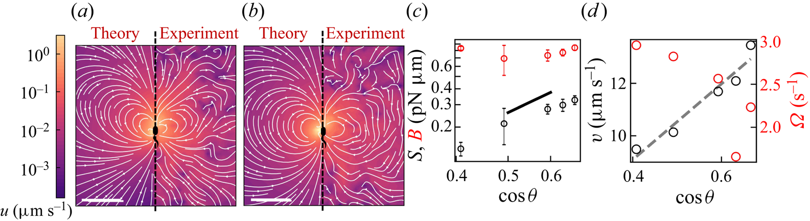
Figure 3. Flow structure depends on the trapped configuration at the interface. (a,b) Plots of the flow fields generated by bacteria with estimated trapping angles (a)  $\theta = 48^{\circ }$ and (b)
  $\theta = 66^{\circ }$. In each plot, the prediction is shown on the left and the observed field is shown on the right. The heat map and streamlines show the magnitude and direction of the flow, respectively, and the scale bar measures
  $20\ \mathrm {\mu }{\rm m}$. (c) Plots of the strength of the
  $\boldsymbol {B}$ (red circles) and
  ${\boldsymbol{\mathsf{S}}}$ (black circles) modes versus
  $\cos \theta$. The vertical error bar represents the fitting error for
  $\boldsymbol {S}$ and
  $\boldsymbol {B}$ modes. The black solid line is a line of slope 2. (d) Plots of the swimming speed (black circles) and angular speed (red circles) versus
  $\cos \theta$. The dashed line is a prediction based on force and torque balances,
  $v\approx v_{max}\cos {\theta }$.
These changes in the balance of the two modes are accompanied by other changes in swimmer dynamics. For example, a dependence on swimming speed  $v$ with
  $\theta$ is readily apparent; we find that
 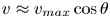 $v\approx v_{max}\cos {\theta }$, where
  $v_{max}=14.5\ \mathrm {\mu }{\rm m}\ {\rm s}^{-1}$ is the maximum speed of the bacteria with the most parallel configuration (figure 3d). This dependence is in keeping with a force balance on a bacterium (figure 2a), which demands that the component of the propulsive force parallel to the interface
  $F_{P\parallel }=F_P\cos \theta$ is balanced by the drag on the swimmer
  $F_D=c_Dv$, where
  $c_D$ is the translational drag coefficient. We find that the angular velocity (i.e. the product of trajectory curvature and speed) measured from swimmer trajectories
  $\varOmega$ also varies strongly with
  $\theta$ (figure 3d), which can be rationalized by a torque balance on a bacterium at the interface. The parallel component of the torque generated from flagellar rotation is balanced by the capillary torque, as rotation in the interfacial plane is precluded by contact-line pinning. The normal component of the torque induced by flagellar rotation
 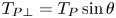 $T_{P\bot }=T_P\sin \theta$ generates rotation of the bacterium perpendicular to the interfacial plane. In addition to this effect, the hydrodynamic torque arising from asymmetric stresses on the swimmer near the interface can also contribute to its rotational behaviour, causing the swimmers to move in circular paths (Deng et al. Reference Deng, Molaei, Chisholm and Stebe2020).
6. Discussion
In this study, we show that the highly anisotropic environment of fluid interfaces generates unique physics that traps bacteria in the interfacial plane in diverse configurations, provides additional forms of dissipation via Marangoni stresses, and alters fundamentally the flow generated by swimmers moving in the pusher mode. This finding is significant, as fluid interfaces occur widely in nature, in medical settings, and in industrial settings. For example, air–water interfaces are encountered in puddles, lakes and larger bodies of water, and oil–water interfaces are encountered for naturally occurring oil seeps and oil spills. Understanding the swimmers’ flow fields is essential for understanding mixing, scattering and collective behaviours generated by micro-swimmers in interfacial active suspensions. In medicine, fluid interfaces are encountered in many organs (e.g. eyes and lungs), in exposed wounds, and on medical equipment. In chemical engineering practice, fluid interfaces are encountered widely in chemical processes, including in membrane reactors designed for simultaneous reaction and separation, and bubbles, emulsions and Pickering emulsions encountered in pharmaceuticals and personal care products. While current practice has focused on passive colloids at interfaces in these settings, understanding the dynamics of active colloidal suspensions at fluid interfaces could generate new strategies to promote mixing using biomimetic active colloids (Fei, Gu & Bishop Reference Fei, Gu and Bishop2017). An important feature of fluid interfaces is the juxtaposition of two fluids with differing viscosities. Hydrodynamic theory predicts that swimming bacteria in bulk phases are attracted hydrodynamically to fluid interfaces (Lopez & Lauga Reference Lopez and Lauga2014; Berke et al. Reference Berke, Turner, Berg and Lauga2008); this attraction may promote bacterial adsorption to the interfaces. In our prior research, we have studied the motion of bacteria at fluid interfaces with viscosity ratios of super-phase: water phase  $\lambda$ ranging from 0 to 300 (Deng et al. Reference Deng, Molaei, Chisholm and Stebe2020). For
  $\lambda \geq 20$, the majority of the interfacially trapped bacteria do not exhibit active motion and display only Brownian displacement. However, for
  $0 \leq \lambda \leq 10$, the probability of swimming in curly trajectories (i.e. in pusher or puller modes) stays approximately constant, indicating that the flow fields measured here may occur at such interfaces. The measurement of swimmers’ flow fields on interfaces with differing viscosity ratios is an open issue.
We have measured the flow field around P. aeruginosa in the pusher mode of swimming. However, unlike swimmers in the bulk, the flow field generated by a puller bacterium is not that of a pusher in reverse. In our prior work, we analysed the trajectories of monotrichous bacteria that swim in pusher and puller modes, and that switch between them by changing the direction of rotation of their single flagellum (Deng et al. Reference Deng, Molaei, Chisholm and Stebe2020). Our data suggest that swimming in puller mode does not solely reverse the direction of swimming from that of a pusher, but that swimming in puller mode is accompanied by changes of the bacterium's body configuration at the interface. In our research, we differentiate between the two modes by observing the curvature of the swimmers’ paths in the interface. Bacteria swim along weakly curved CW paths in pusher mode (viewed from the water side), and after switching move along CCW paths in the puller mode. The pusher segments of the bacteria trajectories have nearly fixed curvatures, suggesting a fixed configuration with respect to the interface. However, trajectories of bacteria moving in puller mode have curvatures that increase gradually, eventually allowing the cells to translate only weakly and to move with high rotational velocities (see figures 4a,b). We hypothesize that these features of the pullers’ trajectories are related to the reorientation of the bacterial flagellum. The flagellum reorientation might result from a hydrodynamically induced torque that bends the flagellar hook and pivots the flagellum away from the interfacial plane in the puller mode, as shown schematically in figure 4(c).
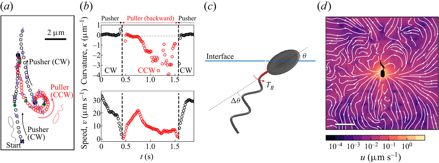
Figure 4. (a) Trajectory of a PA01 bacterium switching between CW rotation (pusher) and CCW rotation (puller) measured over a 2 s time interval. Switching events are marked by black cross symbols. (b) Trajectory curvature and speed versus time for the bacterium trajectory shown in (a). (c) Schematic of an interfacially trapped bacterium in the puller mode. A reorientation torque  $T_R$ due to the hydrodynamic asymmetric dipolar mode at the interface is hypothesized to bend the hook away from the interface. This effect would change the angle of the flagellum by some amount
  $\Delta \theta$. (d) Velocity field measured via CDV around an ensemble of pullers from segments of swimmers’ trajectories with CCW curvature; the median trajectory curvature is
  $0.38\ \mathrm {\mu }{\rm m}^{-1}$. The scale bar is
  $10\ \mathrm {\mu }{\rm m}$.
Analysis of the velocity field of tracer particles around an ensemble of pullers in a common frame indicates that this field differs significantly from that generated by pushers (see figure 1d). In particular, the symmetries with respect to the translational axis that are present in the pusher mode are lacking in the puller mode.
7. Conclusion
We measure the interfacial flow generated by a pusher bacterium, which has striking asymmetries that differ significantly from flows generated by pushers in bulk fluids. The flow is described by two interfacial hydrodynamic dipolar modes: an interfacial stresslet, or  ${\boldsymbol{\mathsf{S}}}$ mode, corresponding to a parallel force dipole on the interface, and a bulk forcing or
  $\boldsymbol {B}$ mode that relies on thrust from the immersed flagellum below the interface that is resisted by stresses in the interface. This latter mode, unique to incompressible interfaces, alters the flow structure significantly, introducing the broken symmetries absent for swimmers in the bulk. The magnitude of the
  ${\boldsymbol{\mathsf{S}}}$ mode depends strongly on the swimmer's trapped configuration, while that of the
  $\boldsymbol {B}$ mode does not.
We have focused on the flow in the plane of the fluid interface. The form of the flow field in planes adjacent to the interface or normal to the interface and their effects on mixing remain unexplored. While theory indicates that the  ${\boldsymbol{\mathsf{S}}}$ mode generates a three-dimensional lamellar flow with no normal component, the
  $\boldsymbol {B}$ mode induces a more complex non-lamellar three-dimensional flow. In addition, an interfacially trapped bacterium is predicted to generate an additional pumping hydrodynamic mode with no interfacial flow that can promote mixing adjacent to the interface, which is also unexplored. The implications of these flow fields in generating active interfaces to promote mixing in the interface and adjacent phases remain to be probed.
Supplementary material
Supplementary material is available at https://doi.org/10.1017/jfm.2023.905.
Acknowledgements
We gratefully acknowledge Dr Z. Ren's help in imaging PA01 on agarose gels.
Funding
This research was made possible by a grant from the National Science Foundation (NSF grant nos DMR-1607878 and CBET-1943394).
Declaration of interests
The authors report no conflict of interest.


 Open access