


1. Introduction
The dynamics of waves and jets at geophysical scales has been of recurrent interest. The study by Miles (Reference Miles1968), for example, refers to an insightful quote from Van Dorn (Reference Van Dorn1968): ‘…the concentric circulate ridges that surround the crater Orientale at lat.  $20^{\circ }$S and long.
  $95^{\circ }$W on the moon may have been initiated as gravity waves on a viscous liquid under the impact of a meteorite’. Miles (Reference Miles1968) subsequently presents an analytical solution to the viscous, linear, Cauchy–Poisson problem motivated by the need to validate this hypothesis. The inviscid, irrotational, linear, Cauchy–Poisson initial value problem (IVP) and its solution (Cauchy Reference Cauchy1816; Poisson Reference Poisson1818) governing linear wave evolution on a pool of deep liquid was reported more than one hundred and fifty years before the viscous extension to the same by Miles (Reference Miles1968) for a localised surface perturbation. Our topic of interest here is the gravity-induced collapse of a large cavity and a resultant (Worthington-like) jet which may be ejected during such collapse, at scales large enough to be geophysically relevant. As will be seen below, the Cauchy–Poisson (CP hereafter) linear solution provides a useful reference, against which the formation of this jet may be compared. Throughout this study, when we characterise lengths to be large, this is relative to both the capillary length scale (
 $\approx$2.7 mm) as well as the amplitude of the initial perturbation. Relevant non-dimensional numbers are quoted appropriately.
Jets can often be seen associated with waves at geophysical scales. For example, numerical models of asteroid impact often depict the generation of a thin ejecta sheet shooting upwards due to impact; see Range et al. (Reference Range2022, figure 1(a)). This sheet may be treated as being similar to a Worthington jet (in two dimensions) and can be modelled as an infinitely tall spike of cross-sectional area  $A_0$. Within the CP linear framework, one can ask what surface waves may be produced due to this ejecta sheet? As explained by Lamb (Reference Lamb1924) (sections 238–241) for the infinite depth case and also by Pidduck (Reference Pidduck1912), the air–water interface represented by the variable
  $\hat {\eta }(\hat {x},\hat {t})$ (
 $\hat {x}$ is the direction of wave propagation and
  $\hat {t}$ is time) becomes wavy due to such an initial disturbance and evolves self-similarly under acceleration due to gravity
  $g$. The evolution is predicted by the CP solution as
 \begin{equation} \frac{{\rm \pi} \hat{x}\hat{\eta}(\hat{x},\hat{t})}{A_0} = f\left(\frac{g\hat{t}^2}{2\hat{x}}\right),\end{equation}
where the functional form of  $f({\cdot })$ in (1.1) is provided by Lamb (Reference Lamb1924). In contrast to the two-dimensional description above, our interest here lies in axisymmetric, surface gravity waves and jets produced therein, in cylindrical geometry. In cylindrical coordinates, for an initial surface perturbation
  $\hat {\eta }(\hat {r},\hat {t}=0)$ (with
 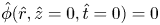 $\hat {\phi }(\hat {r},\hat {z}=0,\hat {t}=0)=0$, where
  $\hat {r}$ is the radial coordinate,
  $\hat {\eta }$ represents the perturbation of the free surface and
  $\hat {\phi }$ is the perturbation velocity potential) on a radially unbounded pool of infinite depth, the classical solution to the linearised CP problem predicts (Debnath Reference Debnath1994)
 \begin{equation} \hat{\eta}(\hat{r},\hat{t})=\int_{0}^{\infty}{\rm d}k\, kJ_0(k\hat{r})\mathbb{H}[\hat{\eta}(\hat{r},0)]\cos (\sqrt{gk}\hat{t}). \end{equation}
Here,  $\mathbb {H}[{\cdot }]$ represents the zeroth-order Hankel transform,
  $J_0({\cdot })$ is the zeroth-order Bessel function of the first kind and
  $k$ represents wavenumber. When the initial surface perturbation,
  $\hat {\eta }(\hat {r},\hat {t}=0)$, has a finite width (i.e. has a characteristic length scale), the CP integral in (1.2) needs to be evaluated numerically and, unlike (1.1), does not lead to self-similar evolution of the interface. We are specifically interested here in initial conditions (i.e.
  $\hat {\eta }(\hat {r},0)$) which lead to jets, yet are simple enough to permit analytical progress into the nonlinear regime. For such initial conditions, we aim to go beyond the linear regime dictated by (1.2) and solve the weakly nonlinear, axisymmetric CP initial-value problem to understand what aspects of jet formation are contained in such an analytical solution.
1.1. Jets from initial surface deformations
Figure 1 depicts two such jets obtained from different initial conditions in axisymmetric geometry. Figure 1(a) depicts a cavity at an air–water interface (blue curve) which has been generated starting from an axisymmetric hump (crest, see inset of figure 2a), by solving the incompressible Euler equations with gravity (and zero surface tension) using the open-source code Basilisk (Popinet Reference Popinet2014). The cavity relaxes producing a Worthington-like jet, indicated by the red curve in this figure. The initial hump is given by the formula  $\hat {\eta }(\hat {r},0)=\hat {a}_0\exp (-{\hat {r}^2}/{\hat {d}^2})[1-({\hat {r}}/{\hat {d}})^2]$,
  $\hat {a}_0$,
  $\hat {d} > 0$ with characteristic height
  $\hat {a}_0$ and width
  $\hat {d}$ (see inset of figure 2a). Figure 1(b), however, also depicts a Worthington jet (red) but is obtained from the relaxation of a nearly spherical cavity (blue), representative of a bubble bursting at an air–water interface (flat line in blue) for low Bond number with zero viscosity. One notes the generation of jets in both situations despite the nearly three orders of magnitude length scale separation and different initial conditions. These jets share qualitatively similar features: the one in figure 1(a) rises significantly beyond its maximum initial amplitude (unity in non-dimensional scale). Similarly, for the jet in figure 1(b), as already noted by Gordillo & Rodríguez-Rodríguez (Reference Gordillo and Rodríguez-Rodríguez2019, p. 557), last paragraph, the droplet ejection velocity from such a jet can be up to twenty times the capillary velocity based on the initial bubble radius.

Figure 1. Jet formation due to cavity relaxation at length scales separated by approximately three orders of magnitude. (a) A cavity (blue) at an air–water interface generated numerically (Popinet Reference Popinet2014) from an initial hump (see inset of figure 2a) of the form  $\eta \equiv {\hat {\eta }(\hat {r},0)}/{\hat {a}_0} = \exp (-r^2)[1-r^2]$ with
  $r \equiv {\hat {r}}/{\hat {d}}$, non-dimensional parameters
 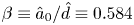 $\beta \equiv {\hat {a}_0}/{\hat {d}} \equiv 0.584$ and Bond number
  $Bo=\infty$ (zero surface tension). Here
  $\hat {r}$ is the radial coordinate,
  $\hat {a}_0$ is measure of the initial hump amplitude and
  $\hat {d}$, a measure of its width. A jet (red curve) is formed due to the relaxation of the cavity, rising sharply upwards at the symmetry axis,
  $\hat {r}=0$. (b) A tiny bubble (blue) of radius
  $\hat {r}_c = 8.57\times 10^{-3}$ cm (Bond number
  $Bo \equiv {\rho g \hat {r}_c^2}/{T}=0.001$, where
  $T$ is surface tension,
  $\rho$ is the water density and
  $g$ is gravity) at the air–water interface whose collapse produces a jet (red curve) (Gordillo & Rodríguez-Rodríguez Reference Gordillo and Rodríguez-Rodríguez2019; Duchemin et al. Reference Duchemin, Popinet, Josserand and Zaleski2002). In (b),
  $\eta \equiv {\hat {\eta }}/{\hat {r}_c}$ and
  $r \equiv {\hat {r}}/{\hat {r}_c}$ (variables with hats are dimensional) where
  $\hat {r}_c$ is the radius of the bubble. Due to the length scale disparity between (a) and (b), the cavity relaxation is dictated nearly entirely by gravity in (a) and almost entirely by surface tension in (b). The dimensional width of the cavity in (a) (blue curve) is
  $\approx$60 cm compared with the bubble diameter (blue curve) in (b) which is
  $2\hat {r}_c \approx 1.714 \times 10^{-2}$ cm. The (non-dimensional) time corresponding to the jet (red curve) in (a) is
 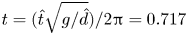 $t ={(\hat {t}\sqrt {g/\hat {d}})}/{2{\rm \pi} } = 0.717$. In (b), the non-dimensional time corresponding to the jet (red curve) is
  $t ={(\hat {t}\sqrt {T/\rho \hat {r}_c^3})}/{2{\rm \pi} } = 0.0963$. Note that the simulation in (a) is started from a crest (inset of figure 2a) unlike the trough-like initial shape of the bubble in (b). Thus, a difference of approximately
  $0.5$ is expected in the non-dimensional time of jet formation between (a) and (b).
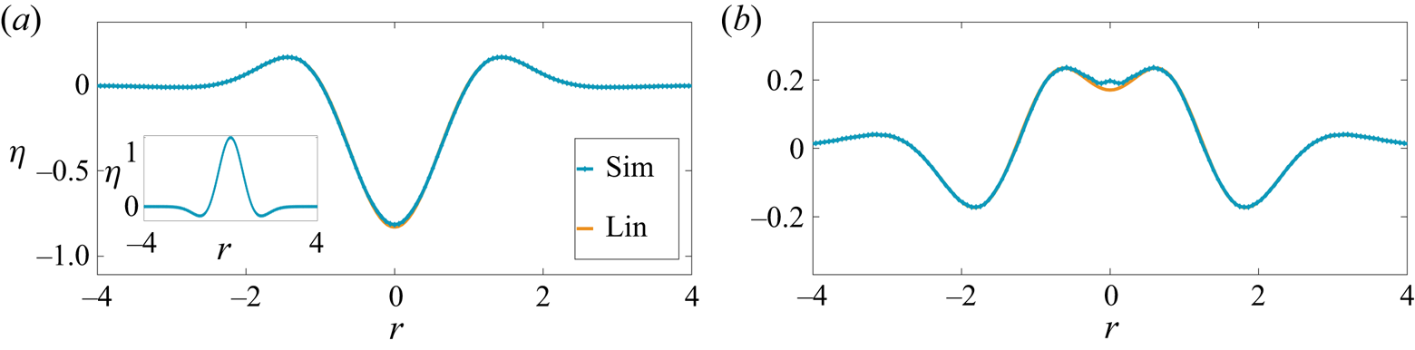
Figure 2. Linear evolution of a cavity from a hump of the initial form  $\eta \equiv {\hat {\eta }(\hat {r},0)}/{\hat {a}_0}=\exp (-r^2)[1-r^2]$,
  $r \equiv {\hat {r}}/{\hat {d}}$. In CGS units,
  $\hat {a}_0=0.54$,
  $\hat {d}=25$,
  $\beta \equiv {\hat {a}_0}/{\hat {d}}=0.0216 \ll 1$. (a)
  $\hat {t}=0.32$ s when a cavity is formed from the initial perturbation (shown in inset). Lin is the linear prediction obtained from expression (1.2). (b) Downward motion of a bump formed at the symmetry axis. Note the very good agreement between simulations and the linear CP prediction. The physical parameters are chosen corresponding to air and water. (a)
  $t ={\hat {t}\sqrt {g/\hat {d}}}/{2{\rm \pi} } = 0.314$ and (b)
  $t ={\hat {t}\sqrt {g/\hat {d}}}/{2{\rm \pi} } =0.717$.
The initial condition which is used to generate the jet in figure 1(a) was proposed by Miles (Reference Miles1968) and represents a volume conserving, free-surface deformation. The linear dimensions of this perturbation (see figure 3 captions for parameter values) was chosen in the simulation to be far greater than the capillary-gravity length ( $2.7$ mm) for air–water. The cavity is thus expected to relax dominantly under the influence of gravity with surface tension playing a relatively insignificant role, particularly in the early stage of relaxation, thereby justifying our neglect of surface tension in the simulation. When the non-dimensional aspect ratio of the cavity
  $\beta \equiv {\hat {a}_0}/{\hat {d}_0} \ll 1$, the collapse is a linear process governed by the CP solution in (1.2). This is seen from the excellent agreement in figure 2(a,b) between numerical simulations and linearised prediction from solving the integral in (1.2) numerically. In contrast, when
  $\beta$ is increased to
  ${O}(1)$, the cavity collapse once again generates a bump earlier, but which now evolves into a thin, sharply shooting jet. This is shown in figure 3(b). As noted earlier, this jet rises significantly higher (
 $\approx$20 cm s, see figure 3b) compared with the initial hump height
  $\hat {a}_0=14.6$ cm. In this case, the temporal evolution is distinctly nonlinear as seen from the rather poor match observed between the numerical simulations and the CP linear solution (1.2) (indicated as ‘Lin’ in the figure legend).

Figure 3. Nonlinear evolution of a cavity starting from a hump of the same form as inset of figure 2(a) with parameters (CGS)  $\hat {a}_0=14.6$,
  $\hat {d}=25$,
 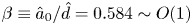 $\beta \equiv {\hat {a}_0}/{\hat {d}}=0.584 \sim {O}(1)$. Note the formation of a slender jet in (b) which rises significantly beyond the initial perturbation amplitude
  $\hat {a}_0$. (a)
  $t ={\hat {t}\sqrt {g/\hat {d}}}/{2{\rm \pi} } =0.314$ and (b)
  $t ={\hat {t}\sqrt {g/\hat {d}}}/{2{\rm \pi} } =0.717$.
1.2. Literature survey: initial value problems (IVPs)
These numerical results, presented in figure 3, emphasise the need for solving the nonlinear CP problem (i.e. predictions beyond (1.2)) for a prescribed surface deformation  $\hat {\eta }(\hat {r},0)$ and zero surface potential
  $\hat {\phi }(\hat {r},\hat {z}=0,\hat {t}=0)=0$, particularly when one seeks a first-principles understanding of the generation mechanism of the jet seen in figure 3(b). The theory literature on the solution to such IVPs particularly in axisymmetric coordinates is quite sparse with the bulk of the rich analytical work being focused on understanding of time-periodic, nonlinear, standing (Strutt Reference Strutt1915) or travelling wave solutions (Stokes Reference Stokes1847, Reference Stokes1880). Commencing from these seminal studies (Stokes Reference Stokes1847; Strutt Reference Strutt1915), a rich literature has since developed on finite amplitude, time-periodic surface waves, both in two-dimensional coordinates (Penney et al. Reference Penney, Price, Martin, Moyce, Penney, Price and Thornhill1952; Taylor Reference Taylor1953; Tadjbakhsh & Keller Reference Tadjbakhsh and Keller1960; Fultz Reference Fultz1962; Schwartz & Whitney Reference Schwartz and Whitney1981; Schwartz & Fenton Reference Schwartz and Fenton1982; Dalzell Reference Dalzell1999) as well as cylindrical, axisymmetric coordinates (Mack Reference Mack1962; Tsai & Yue Reference Tsai and Yue1987). Additionally, several studies of the stability of these finite amplitude solutions (Benjamin & Feir Reference Benjamin and Feir1967; Mercer & Roberts Reference Mercer and Roberts1992) have also been reported.
Here our focus, however, is not on these aforementioned time-periodic solutions but rather on those initial surface deformations which generate a sharply shooting jet, viz. one which rises significantly higher than its parent perturbation, similar to the one seen in figure 3(b). An additional requirement is that the prescribed initial surface deformation  $\hat {\eta }(\hat {r},0)$ should be simple enough to permit analysis in the nonlinear regime, at least perturbatively. The initial condition presented by Miles (Reference Miles1968) and discussed earlier in figures 2 and 3 excites a continuum of modes (radially) initially. Extending the surface response due to such an initial perturbation beyond the CP linear regime described by (1.2) is technically demanding; this is mainly due to the necessity of accounting for interactions of a continuum of modes, interacting quadratically in a radial, axisymmetric geometry. In further analysis, we opt instead to study an alternative and apparently simpler initial condition in a radially confined geometry. The confinement assumption is mainly for analytical ease as it causes the radial part of the spectrum to be discrete instead of continuous.
In the initial condition that we study here, the free surface of a pool of very large depth (compared with the wavelength of the surface perturbation) is deformed at time  $\hat {t}=0$ as a single (radial) eigenmode to the cylindrical, axisymmetric, Laplacian operator, i.e. the zeroth-order Bessel function. This surface deformation thus has the form
  $\hat {\eta }(\hat {r},0)=\hat {a}_0J_0(l_q({\hat {r}}/{\hat {R}_0}))$, with
  $\hat {a}_0$ being the initial perturbation amplitude,
  $\hat {r}$ the radial coordinate,
  $\hat {R}_0$ being the domain radius and
  $l_q$ (
 $q=1,2,\ldots$) a root of the Bessel function
  $\mathbb {J}_1({\cdot })$, this being necessary to satisfy no-penetration at the domain boundary. The length scales are chosen appropriately: the domain radius
  $\hat {R}_0$ as well as the width of the initial perturbation around the symmetry axis (
 ${\approx }2{\rm \pi} \hat {R}_0l_q^{-1}$) are chosen to be quite large, i.e.
  $6$ m and
  $\approx$0.4 m, respectively, compared with the capillary-gravity length scale of 2.7 mm for the air–water interface (see figure 4). At sufficiently large
  $\hat {a}_0$ (>18 times the air–water capillary length, see table 1), numerical simulation of the incompressible Euler equation with gravity (and no surface tension) with this initial surface deformation reveals the formation of a sharply shooting jet at the symmetry axis (
 $\hat {r}=0$) in figure 4. We notice the qualitative similarity of this jet to the one seen earlier in figure 3(c), i.e. both rise far beyond their respective initial, maximum perturbation height
  $\hat {a}_0$. We will understand the mechanism of generation of this jet from first principles here by solving the corresponding IVP. To place our current study in perspective, we briefly summarise the literature on initial-value problems below. There are two classes of initial conditions for the solution to the linear CP problem. These are (a) waves are generated from fluid at rest and a specified initial surface deformation (termed the primary CP problem recently by Tyvand, Mulstad & Bestehorn (Reference Tyvand, Mulstad and Bestehorn2021a) and of current interest; (b) waves and fluid motion are generated from a flat surface due to an initial surface impulse (see expressions
  $3.2.10$ and
  $3.2.12$ in Debnath Reference Debnath1994). This is the secondary CP problem (Tyvand et al. Reference Tyvand, Mulstad and Bestehorn2021a).
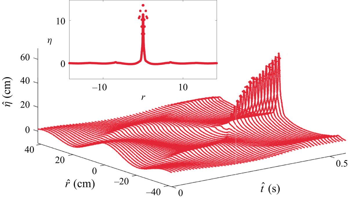
Figure 4. Development of a jet starting from a surface deformation in the shape of single Bessel mode at  $\hat {t}=0$, i.e.
  $\hat {\eta }(\hat {r},0)=\hat {a}_0J_0(l_{35}({\hat {r}}/{\hat {R}_0}))$. The width of the initial hump is
  $\approx$40 cm while the width of the radial domain is
  $\hat {R}_0=600$ cm, only a part of which is shown here. Note that we depict this as a large amplitude perturbation as its non-dimensional steepness
 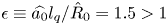 $\epsilon \equiv {\widehat {a_0}l_q}/{\hat {R}_0} = 1.5 > 1$. The resultant jet rises >60 cm at its maximum, far exceeding the initial amplitude
  $\hat {a}_0=8.13$ cm (i.e. approximately seven times the initial perturbation amplitude). Note the formation of droplets from the tip of the jet close to
  $\hat {t}=0.5$ s (non-dimensional
  $t = 6.28$, see (3.1a–c) for temporal scale). The jet profile at
  $\hat {t}=0.58$ s (
 $t=7.81$) is shown in the inset with vertical and horizontal axes non-dimensional as per (3.1a–c). Parameters correspond to Case
  $5$ in table 1. For this simulation,
  $\epsilon =1.5$,
 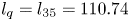 $l_q = l_{35}=110.74$. The drops visible at the tip of the jet in the inset have been manually removed in the main figure.
Table 1. Axisymmetric simulations parameters (CGS units) with air (above)–water (below) parameters conducted in Basilisk (Popinet Reference Popinet2014).  $T$ is the surface tension coefficient,
  $\rho$ is the density of water,
  $\Delta \hat {t}$ is the output time step,
  $\nu$ being the kinematic viscosity of water and
  $g$ is the acceleration due to gravity. All simulations have been conducted with uniform
  $2048^{2}$ grid. Case
  $1$ agrees with linear theory and is not discussed in the text.

The primary and the secondary CP problems in two-dimensional coordinates were investigated numerically using the potential flow equations by Saffman & Yuen (Reference Saffman and Yuen1979). For the latter case, the authors applied a sinusoidal, in space and time, pressure force for a certain duration on a flat interface, and reported the subsequent evolution of the free surface after this forcing was turned off. For the primary CP problem, they used the the finite amplitude solution of Price & Penney (Reference Price and Penney1952) as their initial surface deformation. In both cases, they investigated waves of highest amplitude, obtaining good agreement with the well-known experiments of Taylor (Reference Taylor1953). In two-dimensional Cartesian coordinates, the primary CP problem was subsequently numerically investigated by Longuet-Higgins (Reference Longuet-Higgins2001) and Longuet-Higgins & Dommermuth (Reference Longuet-Higgins and Dommermuth2001b). The authors imposed a prescribed surface deformation in the shape of a circular trough, flanked by circular crests of larger radii. A trough as it collapsed in time was numerically found to generate a jet rising upwards, see Longuet-Higgins & Dommermuth (Reference Longuet-Higgins and Dommermuth2001b, figure 7). Notably, peak accelerations exceeding  $10g$ were observed at the base of their cavity prior to the formation of the jet. In a follow-up work, the secondary CP problem was also investigated numerically by Longuet-Higgins & Dommermuth (Reference Longuet-Higgins and Dommermuth2001a). These authors numerically solved the IVP employing an initial condition, which corresponds to a standing wave solution to the linearised problem. The horizontal (
 $\hat {u}(\hat {x},\hat {z},\hat {t})$) and vertical (
 $\hat {v}(\hat {x},\hat {z},\hat {t})$) components of fluid motion in their simulation were prescribed in two-dimensional coordinates, initially as
  $\hat {u}(\hat {x},\hat {z},0)=C\exp (k\hat {z})\cos (k\hat {x}), \hat {v}(\hat {x},\hat {z},0)=C\exp (k\hat {z})\sin (k\hat {x})$ with the surface being flat initially (
 $\hat {\eta }(\hat {x},0)=0$). For
  $C \ll 1$, a linear standing wave was observed. However, at larger
  $C = O(1)$, the authors reported formation of a jet-like structure at
  $x=0$ during the downward motion of the crest (see Longuet-Higgins & Dommermuth Reference Longuet-Higgins and Dommermuth2001a, figure 9b). Recently, the nonlinear, secondary CP problem in two-dimensional Cartesian coordinates has also been solved analytically, employing small time expansion (Tyvand et al. Reference Tyvand, Mulstad and Bestehorn2021a; Tyvand, Mulstad & Bestehorn Reference Tyvand, Mulstad and Bestehorn2021b). These authors demonstrate significant differences between the linear and the nonlinear CP solution, with increasing amplitude of the initial pressure impulse. However, a clear jet-like structure, analogous to what was presented in the numerical solution by Longuet-Higgins & Dommermuth (Reference Longuet-Higgins and Dommermuth2001a), is not discernable in their figure 6(c) (Tyvand et al. Reference Tyvand, Mulstad and Bestehorn2021a). Of note are also several experimental studies which have investigated the emergence of jets in set-ups which closely resemble the secondary CP problem (i.e. via application of surface impulse), mostly at capillarity dominated length scales. These include the studies by Antkowiak et al. (Reference Antkowiak, Bremond, Le Dizes and Villermaux2007), Bergmann et al. (Reference Bergmann, De Jong, Choimet, Van Der Meer and Lohse2008), Gordillo, Onuki & Tagawa (Reference Gordillo, Onuki and Tagawa2020) of the tubular jet as well as several versions of the so-called Pokrowski's experiment (Lavrentiev & Chabat Reference Lavrentiev and Chabat1980).
The modal initial condition of interest to us in this study, i.e.  $\hat {\eta }(\hat {r},0)=\hat {a}_0J_0(l_q({\hat {r}}/{\hat {R}_0}))$, corresponds to the primary CP problem described above (Tyvand et al. Reference Tyvand, Mulstad and Bestehorn2021a), albeit in cylindrical, axisymmetric coordinates. This initial condition was first studied by Farsoiya, Mayya & Dasgupta (Reference Farsoiya, Mayya and Dasgupta2017) to analytically solve the viscous, linear, IVP at length scales (approximately a few centimetres) chosen such that surface tension as well as gravity were equally important. It was observed in the direct numerical simulations (DNS) reported by Farsoiya et al. (Reference Farsoiya, Mayya and Dasgupta2017) that by systematically increasing the perturbation amplitude
  $\hat {a}_0$, a capillarity-gravity dominated jet emerged at the symmetry axis rising significantly higher than
  $\hat {a}_0$. The viscous, linear theory presented by Farsoiya et al. (Reference Farsoiya, Mayya and Dasgupta2017) was unable to describe the formation of this jet or even account for its inception. In a subsequent study (Basak, Farsoiya & Dasgupta Reference Basak, Farsoiya and Dasgupta2021), the weakly nonlinear solution to the IVP within an inviscid framework and accurate up to
  ${O}(\epsilon ^2)$
  $(\epsilon \equiv {\hat {a}_0 l_q}/{\hat {R}_0})$ corresponding to the same initial condition as that of Farsoiya et al. (Reference Farsoiya, Mayya and Dasgupta2017) was developed. Here too the length scales of interest were similar to that of Farsoiya et al. (Reference Farsoiya, Mayya and Dasgupta2017) with gravity and surface tension forces being equally strong and both forces were accounted for in the theory. This nonlinear theory (Basak et al. Reference Basak, Farsoiya and Dasgupta2021) was a significant improvement over the linear model of Farsoiya et al. (Reference Farsoiya, Mayya and Dasgupta2017) and was able to predict the inception of the jet, comparing well with inviscid simulations of Euler's equations with gravity and surface tension (Basak et al. Reference Basak, Farsoiya and Dasgupta2021). The physical mechanism underlying this jet formation was however not presented by Basak et al. (Reference Basak, Farsoiya and Dasgupta2021). Additionally, for a given choice of
  $l_q$, surface tension and gravity, the analytical theory of Basak et al. (Reference Basak, Farsoiya and Dasgupta2021) becomes singular for certain values of the domain size
  $\hat {R}_0$, this being related to triadic internal resonance. It was demonstrated (Basak et al. Reference Basak, Farsoiya and Dasgupta2021) that these singularities owed their origin to the presence of both surface tension as well as gravity in the theoretical model and represented the cylindrical counterparts of such singularities, better known in the context of Wilton ripples (Wilton Reference Wilton1915) in two-dimensional coordinates.
Now, it is already known from experimental as well as simulation studies on bubble bursting at millimetric (Tagawa et al. Reference Tagawa, Oudalov, Visser, Peters, van der Meer, Sun, Prosperetti and Lohse2012; Deike et al. Reference Deike, Ghabache, Liger-Belair, Das, Zaleski, Popinet and Séon2018; Gordillo & Rodríguez-Rodríguez Reference Gordillo and Rodríguez-Rodríguez2019) and micron length scales (Lee et al. Reference Lee, Weon, Park, Je, Fezzaa and Lee2011) that jets accompany such cavity collapse quite routinely at these scales, where gravity is insignificant compared with surface tension during the collapse. Motivated partly by this observation, simulations of the incompressible, Euler's equation with only surface tension (no gravity) with the aforementioned initial condition of Farsoiya et al. (Reference Farsoiya, Mayya and Dasgupta2017) have been reported recently by Kayal, Basak & Dasgupta (Reference Kayal, Basak and Dasgupta2022). It was demonstrated clearly in these simulations that surface tension alone at sufficiently small scales can produce a jet similar to what was observed at much larger capillary-gravity length scales by Farsoiya et al. (Reference Farsoiya, Mayya and Dasgupta2017) and Basak et al. (Reference Basak, Farsoiya and Dasgupta2021). Concomitantly, the weakly nonlinear solution to the IVP for this initial condition and taking into account only surface tension has also been developed by Kayal et al. (Reference Kayal, Basak and Dasgupta2022). Comparison of this analytical theory against numerical simulations demonstrated very good agreement (Kayal et al. Reference Kayal, Basak and Dasgupta2022), additionally also shedding light into the physical mechanism at work driven by gradients of curvature. It was proven (Kayal et al. Reference Kayal, Basak and Dasgupta2022) that to describe the inception of the jet in the surface tension driven case, one needs to account for nonlinear effects of curvature (the gradient of which drives the flow). To capture this accurately, it was shown that the analytical theory needs to be at least third-order accurate, i.e.  ${O}(\epsilon ^3)$. This third-order accurate solution was reported by Kayal et al. (Reference Kayal, Basak and Dasgupta2022) and has been found to be free from the aforementioned internal resonance related singularities by Basak et al. (Reference Basak, Farsoiya and Dasgupta2021), thereby also alleviating a practical deficiency of the capillary-gravity model studied earlier by Basak et al. (Reference Basak, Farsoiya and Dasgupta2021).
Our present study treats the converse case of Kayal et al. (Reference Kayal, Basak and Dasgupta2022) considering large amplitude surface waves (we typically analyse cases where the initial wave steepness  $\epsilon > 0.5$) under the influence of gravity (and no surface tension, i.e. infinite Bond number). To be consistent, we choose our length scales of interest to be typically in the metre range (radial domain size is
  $6$ m), far greater than the air–water capillary length and this represents a scale up of nearly two orders of magnitude in length, as compared to all our earlier studies (Farsoiya et al. Reference Farsoiya, Mayya and Dasgupta2017; Basak et al. Reference Basak, Farsoiya and Dasgupta2021; Kayal et al. Reference Kayal, Basak and Dasgupta2022). Due to the length scale of our initial perturbation, far exceeding the capillary scale, we expect the relaxation of the perturbation to be dominated by gravity with surface tension playing a negligible role. The motivation to search for jets at such scales comes from the rogue wave literature where a very interesting recent experimental observation of McAllister et al. (Reference McAllister, Draycott, Davey, Yang, Adcock, Liao and van den Bremer2022) reported a ‘spike wave’. McAllister et al. (Reference McAllister, Draycott, Davey, Yang, Adcock, Liao and van den Bremer2022) generate a spike wave which rises up to
  $6$ m in height, via focusing of waves at the symmetry axis of a cylindrical pool. Note that in their case, the focusing was achieved not directly via cavity collapse but via wavemakers at the periphery of a very large cylindrical tank (
 $25$ m diameter) which generated wave components arranged to be in phase at the symmetry axis, leading to a spike wave there. McAllister et al. (Reference McAllister, Draycott, Davey, Yang, Adcock, Liao and van den Bremer2022) also demonstrated that the shape of the spike wave (with the exception of a small region around the symmetry axis) could be accounted for by linear, dispersive focusing. Given our numerical observation of purely capillarity driven jets (sans gravity) for the surface deformation
  $\hat {\eta }(\hat {r},\hat {t}=0)=\hat {a}_0J_0(l_q({\hat {r}}/{\hat {R}_0}))$ at millimetric length scales in Kayal et al. (Reference Kayal, Basak and Dasgupta2022), we ask here if gravity acting alone, at typical length scales of tens of metres, may also produce a jet similar to the one previously seen by us (Kayal et al. Reference Kayal, Basak and Dasgupta2022), employing the same initial condition. We also note here that the experimental study by McAllister et al. (Reference McAllister, Draycott, Davey, Yang, Adcock, Liao and van den Bremer2022) demonstrated recently that similar waves, purely due to gravity, may be generated via focusing. We will show here, theoretically and computationally, that the answer to our question is in the affirmative and also explain the physical mechanism at work. Analogous to the purely surface tension driven, nonlinear theory developed by us in Kayal et al. (Reference Kayal, Basak and Dasgupta2022), the purely gravity driven, second-order, nonlinear theory developed here is devoid of singularities, arising from internal resonance. This theory developed via multiple scale analysis is then compared with numerical simulations obtaining very good agreement.
2. Physical mechanism of jet formation: wave focusing
Figure 5, illustrated further in Appendix C, depicts the radially inward motion of the crests, highlighted by horizontal arrows. To understand physically this radially inward motion seen in figure 5 (Appendix C), we shall employ mass conservation via the kinematic boundary condition. Recall that the solution to the linear CP problem provided in (1.2) for the modal surface deformation, i.e.  $\hat {\eta }(\hat {r},\hat {t}=0)=-\hat {a}_0J_0(l_q({\hat {r}}/{\hat {R}_0}))$ and
  $\hat {\phi }(\hat {r},\hat {z}=0,0)=0$ (
 $\hat {a}_0 > 0$), is
 \begin{gather} \hat{\eta}(\hat{r},\hat{t}) ={-}\hat{a}_0J_0\left(l_q\frac{\hat{r}}{\hat{R}_0}\right)\cos\left(\sqrt{l_q \frac{g}{\hat{R}_0}}\hat{t}\right), \end{gather}
 \begin{gather}\hat{u}_z(\hat{r},\hat{z},\hat{t}) =\frac{\hat{a}_0l_q^{1/2}g^{1/2}}{R_0^{1/2}}J_0\left(l_q\frac{\hat{r}}{\hat{R}_0}\right) \exp\left(l_q\frac{\hat{z}}{\hat{R}_0}\right)\sin\left(\sqrt{l_q \frac{g}{\hat{R}_0}}\hat{t}\right), \end{gather}
 \begin{gather}\hat{u}_r(\hat{r},\hat{z},\hat{t}) ={-}\frac{\hat{a}_0l_q^{1/2}g^{1/2}}{R_0^{1/2}}J_1\left(l_q\frac{\hat{r}}{\hat{R}_0}\right) \exp\left(l_q\frac{\hat{z}}{\hat{R}_0}\right)\sin\left(\sqrt{l_q \frac{g}{\hat{R}_0}}\hat{t}\right), \end{gather}
where  $\hat {u}_r$ and
  $\hat {u}_z$ are the radial and axial components of perturbation velocity. Here a negative sign is deliberately used in the prescription for
  $\hat {\eta }(\hat {r},\hat {t}=0)$ to generate an initial trough (instead of a hump) around
  $\hat {r}=0$ resembling locally a cavity around the symmetry axis. The linearised kinematic boundary condition, i.e.
  $({\partial \hat {\eta }}/{\partial \hat {t}}) = \hat {u}_z(\hat {z}=0,\hat {r},\hat {t})$, implies that the temporal evolution of the interface (at linear order) is determined only by the vertical component of perturbation velocity
  $\hat {u}_z$ at the undisturbed liquid level
  $\hat {z}=0$. Thus for this initial condition, the zeros of the initial surface deformation, viz. the solution to
  $J_0(l_q({\hat {r}}/{\hat {R}_0}))=0$, behave as nodes (at linear order).

Figure 5. Temporal evolution and development of a jet at the symmetry axis. This is from simulations with  $\epsilon =1.5$,
  $l_q = l_{35}=110.74$ (Case
  $5$ in table 1). The arrows indicate the local direction of motion of the interface at that time instant. The inset is a non-dimensional representation of the main figure.
Let us denote the radial location of the first zero of  $J_0(l_q({\hat {r}}/{\hat {R}_0}))=0$ as
  $\hat {r}^{*}$. Observe from (2.1c) that
  $\hat {u}_r(\hat {r} = \hat {r}^{*},\hat {z}=0,0 < \hat {t} < {\tilde {T}_0}/{4})\neq 0$, being a small negative value in the first quarter of the oscillation cycle with time period
  $\tilde {T}_0$, i.e. the early stages of cavity collapse. Thus, linear theory predicts a radially inward, horizontal velocity at the location
  $\hat {r}=\hat {r}^{*}$, as seen from the negative sign of (2.1c) for
  $\hat {r}=\hat {r}^{*},\hat {z}=0$ and
  $\hat {t} < {\tilde {T}_0}/{4}$. This radially inward velocity affects the solution only at nonlinear order leading to radial inward motion of the first node, as may be seen via consideration of the nonlinear term in the kinematic boundary condition. One can now correlate this radially inward motion of the node, with the radially inward motion highlighted earlier in figure 5 (also see Appendix C). Notably, our allusion to the nonlinear term in the kinematic boundary condition implies that the physical mechanism of inward radial motion of the nodes may be understood purely from a kinematic viewpoint (using only mass conservation) without appealing to forces or pressure gradients, which drive the flow. This thus provides insight into why one should generically expect jets from such large amplitude monochromatic perturbations, independent of whether one is investigating the phenomena at capillarity driven length scales (Kayal et al. Reference Kayal, Basak and Dasgupta2022) or far larger, gravity driven scales as is our present case.
Our analytical argument above complements the well accepted viewpoint that these jets are a consequence of flow focusing and thus appear in a wide range of situations. Examples include large cavity collapse (Ghabache, Séon & Antkowiak Reference Ghabache, Séon and Antkowiak2014), impact-driven liquid jets (Antkowiak et al. Reference Antkowiak, Bremond, Le Dizes and Villermaux2007), needle-less injection (Tagawa et al. Reference Tagawa, Oudalov, Visser, Peters, van der Meer, Sun, Prosperetti and Lohse2012) or collapse in granular jets (Lohse et al. Reference Lohse, Bergmann, Mikkelsen, Zeilstra, Van Der Meer, Versluis, Van Der Weele, van der Hoef and Kuipers2004).
3. Weakly nonlinear theory: multiple scale approach
In this section, we develop an  ${O}(\epsilon ^2)$ weakly nonlinear theory employing the method of multiple scales and
  $\epsilon \equiv {\hat {a}_0l_q}/{\hat {R}_0}$ as perturbation parameter to predict from first principles how the jet develops. Note that in our earlier studies (Basak et al. Reference Basak, Farsoiya and Dasgupta2021; Kayal et al. Reference Kayal, Basak and Dasgupta2022), we have used the closely related method of strained coordinates (Lindstedt–Poincare technique). Our usage of multiple scales here is motivated by the fact that at sufficiently early time, the effect of nonlinearity should be small and the interface should behave as a linear standing wave. At a longer time window, however, the effect of nonlinearity becomes apparent including the production of free and bound mode components absent initially. We derive here the amplitude equations governing the modulation of the primary mode as this was not obtained earlier in the strained coordinate method (Basak et al. Reference Basak, Farsoiya and Dasgupta2021; Kayal et al. Reference Kayal, Basak and Dasgupta2022). As our study is restricted to jets on a water pool only, for pure water, the corresponding viscous-gravity length scale
  $(\nu ^2/g)^{1/3}\ll 1$ mm is quite small compared to the length scales of interest to us here. Consequently, we resort to the inviscid, irrotational, potential flow approximation as is standard practise in analysing large-scale surface gravity waves (McAllister et al. Reference McAllister, Draycott, Davey, Yang, Adcock, Liao and van den Bremer2022). These potential flow equations are non-dimensionalised using the following scales:
 \begin{equation} (r,z, \eta) \equiv \frac{l_q}{\hat{R}_0}(\hat{r},\hat{z},\hat{\eta}), \quad t \equiv {\left(l_q\frac{g}{\hat{R}_0}\right)}^{1/2}\hat t, \quad\phi \equiv {\left(\frac{ l_q^3}{\hat{R}_0^3g}\right)}^{1/2}\hat \phi, \end{equation}
which yields the following set of equations written in axisymmetric, cylindrical coordinates. Here (non-dimensional)  $\phi$ represents the disturbance velocity potential and (non-dimensional)
  $\eta$ represents the disturbed free surface. The governing equations and boundary conditions are
 \begin{gather} \nabla^2\phi = \frac{\partial^2\phi}{\partial r^2} + \frac{1}{r}\frac{\partial\phi}{\partial r} + \frac{\partial^2\phi}{\partial z^2} = 0, \end{gather}
 \begin{gather}\eta + \left(\frac{\partial \phi}{\partial t} + \frac{1}{2} \left(\frac{\partial \phi}{\partial r}\right)^2 + \frac{1}{2}\left(\frac{\partial \phi}{\partial z}\right)^2\right)_{z=\eta}= 0, \end{gather}
 \begin{gather}\frac{\partial\eta}{\partial t} + \left(\frac{\partial \eta}{\partial r}\frac{\partial \phi}{\partial r} - {\frac{\partial \phi}{\partial z}}\right)_{z=\eta}=0, \end{gather}
 \begin{gather}(\phi)_{z\rightarrow -\infty} \rightarrow \text{finite},\quad \left(\frac{\partial \phi}{\partial r}\right)_{r = l_q} = \left(\frac{\partial \eta}{\partial r}\right)_{r = l_q} = 0, \end{gather}
 \begin{gather}\int_{0}^{l_q} {\rm d}r \, r\eta(r,t) = 0, \end{gather}
 \begin{gather}\text{with initial conditions}\quad\eta(r,0) = \epsilon J_0(r), \quad \frac{\partial \eta}{\partial t}(r,0) = 0, \quad \phi(r,z,0) = 0. \end{gather}
Equation (3.2a) is the Laplace equation in cylindrical axisymmetric coordinates, (3.2b,c) are the constant pressure condition (from Bernoulli's equation) and the kinematic boundary condition, respectively, both at the free surface. Equation (3.2d) is the finiteness of the velocity potential at infinite depth (deep water limit is assumed for simplicity). Equation (3.2e,f) are the no-penetration and free-edge boundary conditions at the outer radial boundary  $\hat {r}=\hat {R}_0$. Equation (3.2g) is the overall mass conservation while (3.2h,i,j) are initial conditions corresponding to the primary CP problem.
The number  $l_q$ (
 $q \in \mathbb {Z}^+$) in the initial condition
  $\hat {\eta }(\hat {r},\hat {t}=0)=\hat {a}_0J_0(l_q({\hat {r}}/{\hat {R}_0}))$ satisfies
  $J_1(l_q)=0$. The chosen integer value of
  $q$ in
  $\epsilon \equiv l_q({\hat {a}_0}/{\hat {R}_0})$ is related to the number of extremas of
  $J_{0}$ within the radial domain
  $\hat {R}_0$. The numerical value of
  $\hat {R}_0l_q^{-1}$ provides a rough measure of the wavelength of the initial perturbation while nonlinearity is controlled by the magnitude of the perturbation amplitude
  $\hat {a}_0$ relative to
  $\hat {R}_0l_q^{-1}$. To minimise the effect of the confining radial boundary
  $\hat {R}_0$ on the cavity collapse process, we require
  $\hat {R}_0l_q^{-1} \ll \hat {R}_0$ and this is ensured by choosing
  $l_q \gg 1$. In this study, we choose
  $q=35$ implying
  $l_{35}=110.74$. The variables
  $\phi$,
  $\eta$ and
  $t$ are expanded in a power series in
  $\epsilon$ (
 $\epsilon \ll 1$) for finite
  $l_q$. Employing multiple scale analysis, we replace the temporal dependencies in all dependent variables as
  $T_n \equiv \epsilon ^n t$ (up to second order). Thus, we have up to second order,
 \begin{gather} \phi(r,z,T_0,T_2) = \epsilon\phi_1(r,z,T_0,T_2) + \epsilon^2\phi_2(r,z,T_0,T_2) + {O}(\epsilon^3), \end{gather}
 \begin{gather}\eta(r,T_0,T_2) = \epsilon\eta_1(r,T_0,T_2) + \epsilon^2\eta_2(r,T_0,T_2) + {O}(\epsilon^3), \end{gather}
where  $T_0\equiv t$ and
  $T_2\equiv \epsilon ^2t$. After performing a Taylor series expansion of (3.2b) and (3.2c) about the unperturbed interface
  $z = 0$ and thereafter substituting expansions (3.3) and (3.4) in (3.2a–j), we extract the following set of linear equations governing
  $\phi _i(r,z,T_0,T_2)$ and
  $\eta _i(r,T_0,T_2)$ at the
  $i$th order for all
  $i = 1,2,3,\ldots$. Hence, at every
  ${O}(\epsilon ^i)$ and using the short-hand symbol
  $D_n \equiv {\partial }/{\partial T_n}$, we have
 \begin{gather} \nabla^2\phi_i=0, \end{gather}
 \begin{gather}D_0\phi_i +\eta_i = \mathscr{N}_i(r,T_0,T_2), \quad \frac{\partial \phi_i}{\partial z} - D_0\eta_i = \mathscr{M}_i(r,T_0,T_2) \quad \text{at}\ z = 0, \end{gather}
 \begin{gather}(\phi_i)_{z\rightarrow -\infty} \rightarrow \text{finite},\quad\left(\frac{\partial \phi_i}{\partial r}\right)_{r = l_q} = 0,\quad \left(\frac{\partial \eta_i}{\partial r}\right)_{r = l_q} = 0, \end{gather}
 \begin{gather}\int_{0}^{l_q} {\rm d}r \, r\eta_i(r,T_0,T_2) = 0 \end{gather}
and
 \begin{equation} \eta_i(r,0,0) = \delta_{1i}J_0(r), \quad D_0\eta_i(r,0,0) = 0, \quad \phi_i(r,z,0,0) = 0. \end{equation}
Here,  $\delta _{1i}$ is the Kronecker delta while
  $\mathscr {M}_i(r,T_0,T_2)$ and
  $\mathscr {N}_i(r,T_0,T_2)$ are nonlinear terms involving products of lower-order solutions of
  $\phi _i$ and
  $\eta _i$ with
  $\mathscr {M}_1(r,T_0,T_2)=\mathscr {N}_1(r,T_0,T_2)=0$. Due to this at the linear order, we have a homogeneous set of equations. The expressions for
  $\mathscr {M}_2(r,T_0,T_2),\mathscr {N}_2(r,T_0,T_2)$ as well as
  $\mathscr {M}_3(r,T_0,T_2),\mathscr {N}_3(r,T_0,T_2)$ (necessary for eliminating resonant forcing) are provided in the Appendix. As all
  $\phi _i$ satisfy the Laplace equation (3.5a), we expand
  $\phi _i$ and
  $\eta _i$ at every order in a Dini series (Mack Reference Mack1962) in the following form (note that
  $q$ is a given fixed integer used to indicate the primary Bessel mode that is excited initially):
 \begin{equation} \phi_i(r,z,T_0,T_2) = \sum_{j = 0}^{\infty}p_i^{(\,j)}(T_0,T_2)\exp(\alpha_{j,q} z)J_0(\alpha_{j,q} r)\end{equation}
and
 \begin{align} \eta_i(r,T_0,T_2) = \sum_{j = 0}^{\infty}a_i^{(\,j)}(T_0,T_2)J_0(\alpha_{j,q} r), \quad \alpha_{j,q} \equiv \frac{l_j}{l_q}, \ i=1,2,3,\ j=1,2,3,4\ldots. \end{align}
By construction, each term in the expansion in (3.6) satisfies the Laplace equation (3.5a), while each term in (3.7) satisfies the mass conservation equation (3.5g). In addition, (3.6) and (3.7) together respect the finiteness condition as well as the no-penetration and the free-edge conditions (3.5d,e,f). Our task thus reduces to ensuring that (3.5b,c) are satisfied, and these in turn determine equations governing  $p_{i}^{(\,j)}(T_0,T_2)$ and
  $a_{i}^{(\,j)}(T_0,T_2)$ in the expansions (3.6) and (3.7). These equations have to be solved subject to initial conditions (3.5h,i,j).
Substituting (3.6) and (3.7) into (3.5b,c), taking inner products with  $J_{0}(\alpha _{n, q}) r \,{\rm d}r$ and using the orthogonality relations for Bessel functions (see the supplementary material of Basak et al. (Reference Basak, Farsoiya and Dasgupta2021) for the relevant orthogonality relations), we obtain the following equations at each
  ${O}(\epsilon ^i)$:
 \begin{align} &(D_0^2 + \omega_{j,q}^2 )p_i^{(\,j)}(T_0,T_2)\nonumber\\ &\quad = \frac{2}{l_q^2 J_0^2(l_j)}\int_{0}^{l_q} {\rm d}r\, r J_0(\alpha_{j,q} r) \{D_0\mathscr{N}_i(r,T_0,T_2) + \mathscr{M}_i(r,T_0,T_2) \} \end{align}
and
 \begin{equation} a_i^{(\,j)}(T_0,T_2) = \frac{2}{l_q^2 J_0^2(l_j)}\int_{0}^{l_q} {\rm d}r \, rJ_0(\alpha_{j,q} r) \mathscr{N}_i(r,T_0,T_2) - D_0p_i^{(\,j)}(T_0,T_2).\end{equation}
Here,  $\omega _{j,q}^{2} \equiv \alpha _{j,q}$ is the non-dimensional form of the dispersion law for pure gravity waves on a free surface. Equation (3.8a) is a second-order, partial differential equation which is solved subject to the following initial conditions (these are obtained by substituting (3.6) and (3.7) into initial conditions (3.5h,i,j)):
 \begin{equation} p_i^{(\,j)}(0,0) = 0, \quad D_0p_i^{(\,j)}(0,0) = \frac{2}{l_q^2 J_0^2(l_j)}\int_{0}^{l_q} {\rm d}r \,r J_0(\alpha_{j,q} r) \mathscr{N}_i(r,0,0) - \delta_{1i}\delta_{qj}. \end{equation}
The expression for  $a_i^{(\,j)}(T_0,T_2)$ may then be obtained from (3.8b), knowing the expression for
  $p_i^{(\,j)}(T_0,T_2)$ from the solution to (3.8a).
3.1. Linear solution ( $i=1$)

At  ${O}(\epsilon )$,
  $\mathscr {N}_i(r,T_0,T_2)=\mathscr {M}_i(r,T_0,T_2)=0$ which reduces (3.8a) to a homogeneous equation along with initial conditions obtained from (3.9) for
  $i=1$, i.e.
 \begin{equation} p_1^{(\,j)}(0,0) = 0, \quad D_0p_1^{(\,j)}(0,0) ={-}\delta_{qj}. \end{equation}
This leads to
 \begin{equation} p_1^{(q)}(T_0,T_2) = (\mu_{1q}(T_2)\cos T_0+\nu_{1q}(T_2)\sin T_0)\\ \end{equation}
and
 \begin{equation} \left.\begin{array}{c@{}} a_1^{(q)}(T_0,T_2) = (\mu_{1q}(T_2)\sin T_0-\nu_{1q}(T_2)\cos T_0), \\ p_1^{(\,j)}(T_0,T_2) = 0, \quad a_1^{(\,j)}(T_0,T_2) = 0\quad \forall j\neq q, \end{array}\right\} \end{equation}
where  $\mu _{1q}(T_2)$ and
  $\nu _{1q}(T_2)$ in 3.11 and 3.12 are functions of the slow time scale
  $T_2$ and satisfy initial conditions
  $\mu _{1q}(0)=0$,
  $\nu _{1q}(0)=-1$, obtained from (3.10). Hence at
  ${O}(\epsilon )$,
  $\phi _1$ and
  $\eta _1$ are obtained as
 \begin{equation} \phi_1(r,z,T_0,T_2) = (\mu_{1q}(T_2)\cos T_0+\nu_{1q}(T_2)\sin T_0)J_0(r)\exp (z) \end{equation}
and
 \begin{equation} \eta_1(r,T_0,T_2) = (\mu_{1q}(T_2)\sin T_0-\nu_{1q}(T_2)\cos T_0)J_0(r). \end{equation}
Note that if we were to terminate our calculation at this order, then  $\mu _{1q}$ and
  $\nu _{1q}$ would be treated as constants being
  $\mu _{1q}=0,\nu _{1q}=-1$ and substituting these in (3.13) and (3.14), we obtain the standing wave that is predicted at linear order, i.e.
 \begin{equation} \phi(r,z,T_0) ={-}\epsilon\sin(T_0)J_{0}(r)\exp(z),\quad \eta(r,T_0) = \epsilon\cos(T_0)J_{0}(r). \end{equation}
Equations (3.15) predict that the interface  $\eta$ evolves temporally as a standing wave with unit frequency (in non-dimensional sense). Expectedly, at all time, there is only the primary mode and no transfer of energy to modes other than this mode (index
  $q$) is predicted at this order. Consequently, there is no jet seen in the time evolution of the standing wave. At the axis of symmetry, the initial perturbation represented by
  $\eta$ in (3.15) has an amplitude
  $\epsilon$ at
  $T_0=0$ and after one time period at
  $T_0=2{\rm \pi}$, once again rises to the same amplitude at this location. While we have seen earlier that the radial velocity at the node (
 $r = r^{*}$) is non-zero and radially inward already at this order, this velocity does not affect the time evolution of the standing wave. To theoretically predict the radial inward movement of nodes which leads to the jet seen in figure 4, our calculation must be extended to nonlinear order. We expect to obtain amplitude equations governing
  $\mu _{1q}(T_2)$ and
  $\nu _{1q}(T_2)$ appearing in 3.13 and 3.14 by going up to nonlinear order, and this is presented next.
3.2. Nonlinear solution ($i=2,3$)

On a longer time scale  $T_2$, the amplitude of the primary mode (
  $j=q$) gets modulated, this being dictated by nonlinear equations governing
  $\mu _{1q}(T_2)$ and
  $\nu _{1q}(T_2)$. To determine these equations, it becomes necessary to obtain expressions up to
  ${O}(\epsilon ^3)$ for
  $\mathscr {M}_2$ and
  $\mathscr {N}_2$ as well as
  $\mathscr {M}_3$ and
  $\mathscr {N}_3$), where resonant forcing of the primary mode is encountered and eliminated. The nonlinear calculation proceeds in an analogous manner to the linear one outlined above, although the algebra, expectedly, becomes increasingly tedious. We outline only the important steps here.
For  $i=2$,
  $\mathscr {M}_2(r,T_0,T_2)\neq 0$ and
  $\mathscr {N}_2(r,T_0,T_2)\neq 0$, and expressions for these are provided in the Appendix. As a result, (3.8a) governing
  $p_2^{(i)}(T_0,T_2)$ is an inhomogeneous equation. To prevent very lengthy calculation for solving this equation, we introduce an approximation as follows. While solving (3.8a) for
  $p_2^{(\,j)}(T_2)\;(\,j=0,1,2,3,\ldots )$, constants of integration appear which, strictly speaking, are not constants but functions of the slow time scale
  $T_2$. These govern the modulation of the amplitude of the secondary modes. To determine the equations governing this modulation, one needs to go to higher order (presumably beyond third order). Our purpose here is to obtain a nonlinear approximation which contains enough physics to model the inception of the jet seen earlier. Thus, to prevent very lengthy, higher-order calculations, we ignore the temporal variation of these functions treating them instead as constants to be determined from initial conditions. Our analytical solution thus contains the modulation of the amplitude of the linear solution (i.e. the primary mode with index
  $q$), but neglects amplitude modulation of the secondary modes generated in the spectrum, via nonlinearity. The justification for this will be obtained a posteriori, when we compare our analytical predictions with numerical simulations. After lengthy algebra, the
  ${O}(\epsilon ^2)$ corrections are found to be
 \begin{align} \phi_2(r,z,T_0,T_2) &= \left[\frac{\nu_{1q}(T_2)^2-\mu_{1q}(T_2)^2}{2}\sin (2T_0)+\mu_{1q}(T_2)\nu_{1q}(T_2)\cos (2T_0)\right]J_0^2(l_q)\nonumber\\ &\quad +\sum_{n = 1}^{\infty}[\xi_{n,q}^{(2)}\sin(\omega_{n,q}T_0) + \xi_{n,q}^{(3)}(\mu_{1q}(T_2),\nu_{1q}(T_2))\cos(2T_0) \nonumber\\ &\quad +\xi_{n,q}^{(4)}(\mu_{1q}(T_2),\nu_{1q}(T_2))\sin(2T_0)] \exp(\alpha_{n,q}z)J_0(\alpha_{n,q}r) \end{align}
and
 \begin{align} &\eta_2(r,T_0,T_2) = \sum_{n = 1}^{\infty}[\zeta_{n,q}^{(1)}\cos(\omega_{n,q}T_0) + \zeta_{n,q}^{(3)}(\mu_{1q}(T_2),\nu_{1q}(T_2))\cos(2T_0) \nonumber\\ &\quad +\zeta_{n,q}^{(4)}(\mu_{1q}(T_2),\nu_{1q}(T_2))\sin(2T_0) +\zeta_{n,q}^{(5)}(\mu_{1q}(T_2),\nu_{1q}(T_2))]J_0(\alpha_{n,q}r). \end{align}
 In (3.16),  $\xi _{n,q}^{(1)}=0,\xi _{n,q}^{(2)}$ are constants (part of the complementary function for (3.8a), these being assumed to be constants instead of being functions of
  $T_2$, as explained earlier). Expressions for
  $\xi _{n,q}^{(2)}$,
  $\xi _{n,q}^{(3)}(\mu _{1q}(T_2),\nu _{1q}(T_2))$ and
  $\xi _{n,q}^{(4)}(\mu _{1q}(T_2),\nu _{1q}(T_2))$ are provided in the Appendix. Similarly, in (3.17),
  $\zeta _{n,q}^{(1)}$ and
  $\zeta _{n,q}^{(2)}=0$ are constants while expressions for
  $\zeta _{n,q}^{(3)}(\mu _{1q}(T_2),\nu _{1q}(T_2))$,
  $\zeta _{n,q}^{(4)}(\mu _{1q}(T_2),\nu _{1q}(T_2))$ and
  $\zeta _{n,q}^{(5)}(\mu _{1q}(T_2),\nu _{1q}(T_2))$ are provided in the Appendix. Note that these expressions depend on the unknowns
  $\mu _{1q}(T_2)$ and
  $\nu _{1q}(T_2)$. Equations for these two unknowns are obtained at
  ${O}(\epsilon ^3)$ via elimination of resonant forcing terms for the primary mode.
3.3. Amplitude equation(s)
To obtain the equations governing  $\mu _{1q}(T_2)$ and
  $\nu _{1q}(T_2)$, it is necessary to carry out the calculation till
  ${O}(\epsilon ^3)$ and seek terms which resonate with the primary mode. As the natural frequency on the left-hand side of (3.18a) is unity for
  $j=q$ (
 $\omega _{q,q}^2=1$), we look for terms on the right-hand side in (3.18a) which are proportional to
  $\cos (T_0)$ or
  $\sin (T_0)$. Writing (3.8a) for
  $i=3$ and
  $j=q$,
 \begin{equation} (D_0^2 + 1)p_3^{(q)}(T_0,T_2) = \frac{2}{l_q^2 J_0^2(l_q)}\int_{0}^{l_q} {\rm d}r\, r J_0(r) \{D_0\mathscr{N}_3 + \mathscr{M}_3 \}. \end{equation}
Expressions for  $\mathscr {M}_3(r,T_0,T_2),\mathscr {N}_3(r,T_0,T_2)$ necessary to evaluate the right-hand side of (3.18) are provided in the Appendix. Note in particular that
  $\mathscr {M}_3$ and
  $\mathscr {N}_3$ both contain terms like
  $D_2\eta _1$ and
  $D_2\phi _1$ which lead to time derivatives of
  $\mu _{1q}(T_2)$ and
  $\nu _{1q}(T_2)$. Elimination of the coefficients of
  $\cos (T_0)$ and
  $\sin (T_0)$ appearing on the right-hand side of (3.18) lead us to two nonlinear, coupled ordinary differential equations governing evolution of
  $\mu _{1q}(T_2)$ and
  $\nu _{1q}(T_2)$ over the slow time scale
  $T_2$. The algebra is again quite lengthy and we provide only the amplitude equations here. These are of the form
 \begin{equation} \left.\begin{array}{c} D_2\mu_{1q}=r_1\mu_{1q}+r_2\nu_{1q},\quad D_2\nu_{1q}=r_3\mu_{1q}-r_1\nu_{1q},\\ \quad \mu_{1q}(0) = 0,\ \nu_{1q}(0) ={-}1 \end{array}\right\}. \end{equation}
Here,  $r_{1}$,
  $r_{2}$ and
  $r_{3}$ in (3.19a) and (3.19b) are nonlinear functions of
  $\mu _{1q}$ and
  $\nu _{1q}$ whose expressions are provided in the Appendix. Equations (3.19a) and (3.19b) are solved numerically in MATLAB and together with expressions at linear and quadratic order provided earlier in (3.13), (3.14), (3.16) and (3.17), we obtain a second-order solution to the primary CP problem for our initial condition. This analytical prediction is free from any fitting parameters and is tested against numerical simulations of the incompressible Euler equation with gravity, in the next section.
3.4. Comparison of theory with numerical simulations
In this section, the results from numerical simulations are compared against the theoretical predictions made earlier. To do this, we truncate the infinite series in (3.16) and (3.17) at  $n=70$. This number is twice the index of the primary mode, which in the present study has been chosen to be
  $q=35$. Figure 12 in Appendix B presents the Hankel transform of the interface for
  $\epsilon =0.5$ from our
  ${O}(\epsilon ^2)$ theory, comparing with the Hankel transform of the interface obtained from numerical simulations. This is done at
  $\hat {t}=0.483$ s and the interface at this instant of time is depicted in figure 6(d). It is clearly seen that at this instant of time, when the interface shows more than
  $37\,\%$ overshoot at the symmetry axis (figure 6d), there is a perceptible amount of potential energy around the second harmonic of the primary mode, i.e.
  $q=70$, see inset of figure 12. However, our theoretical model predicts very little potential energy beyond this and consequently, we have truncated our expansion at
  $n=70$ in expressions (3.16) and (3.17).
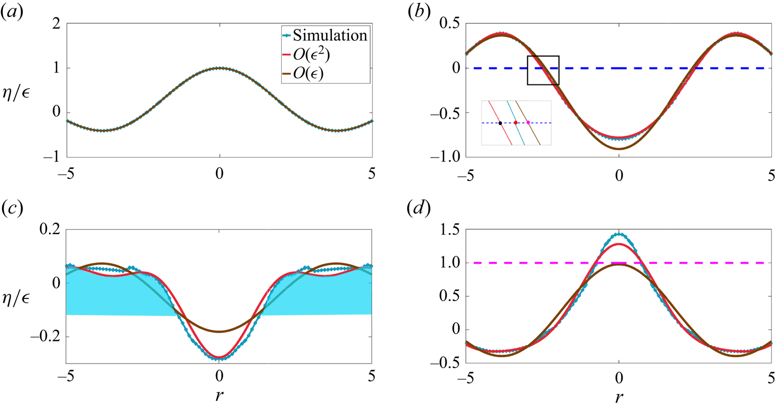
Figure 6. (a–d) Comparison of the interface profile  ${\eta }/{\epsilon }$ at various instants with linear and weakly nonlinear, analytical solutions. Solid red,
  ${O}(\epsilon ^2)$ weakly nonlinear theory; solid brown,
  ${O}(\epsilon )$ linear theory and numerical simulation (Sim, solid blue line) for
  $\epsilon =0.5$ and
  $l_{35}=110.74$ (Case
  $2$ in table 1). (b) Inset depicts a close-up view of the first zero crossing of the perturbed interface. Note the qualitative differences between the simulation and linear theory particularly in (c) and (d). The shaded region in blue in (c) depicts the wave crest whose inward focusing results in an overshoot. Significant overshoot (
 $\approx$37 %) is seen in the numerical simulation, i.e. above the dashed pink line in (d), at
  $r=0$. Unlike linear theory, the weakly nonlinear theory predicts this overshoot nearly correctly as seen in (d). (a)
  $\hat {t}=0$ (non-dimensional
  $t=0$), (b)
  $\hat {t}=0.266$ s (
 $t=3.58$), (c)
  $\hat {t}=0.337$ s (
 $t=5.07$) and (d)
  $\hat {t}=0.483$ s (
 $t=6.5$).
The numerical simulations have been carried out using the open source code Basilisk (Popinet Reference Popinet2014) employing a cylindrical domain of radius  $\hat {R}_0=600$ cm and depth
  $\hat {H}=300$ cm. As the chosen value of
  $q=35$, this implies that the (approximate) wavelength of the initial perturbation is far smaller than
  $\hat {H}=300$, justifying the deep water approximation that we make in our theory. The parameters of various simulations are summarised in table 1. In all simulations, we have employed free-edge boundary conditions at the wall implying that the interface intersects the solid boundary at
  $\hat {R}_0$ at an angle of
  ${\rm \pi} /2$ at all times.
Figure 6 shows the comparison of linear and weakly nonlinear theory with the simulation for  $\epsilon =0.5$. It can be seen that the weakly nonlinear theory captures the simulation profiles quite well. Note in particular figure 6(d), showing clearly that the overshoot seen in the simulation at the symmetry axis over and above unity (pink dashed line in the figure) is predicted well by the
  ${O}(\epsilon ^2)$ theory. This overshoot is the precursor to the slender jet that develops at the axis of symmetry, seen for far larger values of
  $\epsilon =1.5$, please refer to figure 4. Figure 7 shows the inward movement of the first zero crossing of the interface
  $\eta$ (around
  $r=-2.4$ in figure 6b) from panels (b) to (c). Note the good agreement in figure 7 between nonlinear theory and simulation. During this time window, the interface around the axis of symmetry is shaped like a cavity which collapses subsequently, leading to the overshoot seen in figure 6(d). In figure 8, we test the limit of our theory, extending the magnitude of
  $\epsilon$ to
  $0.9$ (Case
  $3$ in table 1). It is seen that although the
  ${O}(\epsilon ^2)$ theory shows the overshoot, it significantly underdescribes the jet being unable to capture its slenderness well. For reference, the initial condition is also provided in this figure in green. This value of
  $\epsilon \sim 0.9$ represents a simulation which lies outside the range of utility of the
  ${O}(\epsilon ^2)$ theory for describing these jets. While the theory is able to describe the inception (up to
  $\epsilon =0.5$), it is unsuitable in this parametric regime where nonlinearity becomes very strong. This regime will be analysed in detail in the next sub-section. We note that the inability of the current multiple scale analysis to capture the overshoot accurately for
  $\epsilon > 0.6$ is unrelated to the approximation discussed above in (3.16). To check this, we have compared our current solution with the stretched coordinate solution reported earlier by Basak et al. (Reference Basak, Farsoiya and Dasgupta2021) (setting surface tension equal to zero in the latter) and found that predictions from the two methods are indistinguishable. Figure 9(a) compares the overshoot seen at the symmetry axis (
 $r=0$) as a function of
  $\epsilon$. This figure demonstrates that the weakly nonlinear theory presented here may be used reliably up to
  $\epsilon \sim 0.6$ beyond which it becomes quite inaccurate. Figure 9(b) demonstrates that the displacement of the tip of the jet, viz.
  $\hat {\eta }(\hat {r}=0,\hat {t})$, displays a parabolic dependence in time, in agreement with the earlier observations of Ghabache et al. (Reference Ghabache, Séon and Antkowiak2014).

Figure 7. Radial inward motion of the first zero crossing between figures 6(b) and 6(c). Note from figure 6 that within this time window, the interface is shaped as a cavity around  $r=0$ and the collapse of this cavity occurs nonlinearly, leading to the overshoot seen in figure 6. As noted earlier, the inward motion of the first zero crossing of
  $\eta (r=r^{*},t)$ may be interpreted as radial inward focusing of the two humps shown earlier in figure 5. As seen, linear theory (pink symbols) does not allow any radial displacement of the zero crossings. However, the weakly nonlinear theory is able to describe the inward motion of the nodes correctly qualitatively, although some quantitative differences persist between theory and simulations. The inset depicts the main figure with dimensional axes.

Figure 8. Interface for  $\epsilon =0.9$,
  $\hat {t}=0.47$ s (non-dimensional
  $t=6.33$) before the maximum height is reached. The
  ${O}(\epsilon ^2)$ theory is unable to describe the slender jet seen in simulations although it manages to get the overshoot correct qualitatively. The line in green represents the initial condition.

Figure 9. (a) Comparison of the maximum height ( $\hat {\eta }_{max}/\hat {a}_0$) at the symmetry axis, as a function of increasing
  $\epsilon$. Note that
  $\eta _{overshoot}\equiv {\hat {\eta }_{max}}/{\hat {a}_0} - 1 = {O}(\epsilon ^2)$ which translates in dimensional variables to
  $\hat {\eta }_{overshoot} \sim {\hat {a}_0^3}/{\hat {R}_0^2}$ (Ghabache et al. Reference Ghabache, Séon and Antkowiak2014). Our weakly nonlinear model estimates the overshoot with an error of <20 % up to
  $\epsilon \sim 0.6$. Up to this
  $\epsilon =0.6$, the shape of the jet in theory and simulation agree reasonably well. Beyond this, the weakly nonlinear model becomes quite inaccurate. Note that the analytical model displays overshoot earlier in time compared with the simulation. The thin blue line indicates the linear solution which does not have any overshoot. The green curve has the equation
  $0.32\epsilon ^2 + 0.19\epsilon + 1.1$ and is obtained by fitting a parabola to the analytical model (diamonds). (b) Variation of non-dimensional amplitude with time at the axis of symmetry. Dots represent simulation data while solid curves are parabolic fits to the same, in qualitative agreement with observations of Ghabache et al. (Reference Ghabache, Séon and Antkowiak2014, figure 2).
We have argued earlier that the development of the jet requires radially inward focusing of surface gravity waves at the axis of symmetry, much akin to the phenomena of bubble collapse albeit at far smaller capillary scales, where radially inward focusing of capillary waves are implicated in the formation of a slender jet (Duchemin et al. Reference Duchemin, Popinet, Josserand and Zaleski2002; Gordillo & Rodríguez-Rodríguez Reference Gordillo and Rodríguez-Rodríguez2019). Predictions from our theoretical model vis-a-vis numerical simulations presented in figure 6, where an inward motion of the first nodes is visible, see panel (b) inset for the weakly nonlinear theory as well as simulations, demonstrate that this radially inward flow focusing at large length scales may also be interpreted as the reason for the generation of jets at these large length scales. Alternatively, this process may also be interpreted as constructive interference at the symmetry axis from a large number of (free) modes in the spectrum. In our study, these free modes are produced via quadratic interactions of the monochromatic initial condition.
3.5. Strongly nonlinear regime, inertial regime
In the previous section, we have studied simulations for  $\epsilon < 1$ and the weakly nonlinear theory was able to describe the inception of the jet up to
  $\epsilon \approx 0.5$. We now move to the strongly nonlinear regime (
 $\epsilon >1$) where, due to stronger nonlinearity, the theory becomes inadequate and a slender jet emerges in the numerical simulations (figure 4). Here, qualitative understanding may be obtained by referring to the analytical solution on hyperboloidal jets by Longuet-Higgins (Reference Longuet-Higgins1983) in axisymmetric, extensional flow. It will be seen that this analytical model of Longuet-Higgins (Reference Longuet-Higgins1983) provides a reasonably good approximation to the jets that arise in our simulations, when
  $\epsilon >1.2$.
Interestingly, this exact solution is singular at  $\hat {t}=0$ where it predicts a divergent velocity (
 $\dot {c}\sim \hat {t}^{-1/3}$) and a divergent acceleration (
 $\ddot {c}\sim \hat {t}^{-4/3}$) at the tip of the free surface shaped as a hyperboloid, viz. at
  $\hat {z}=c(\hat {t})$. In a time window around this initial ‘jerky start’ to motion, the half-angle
  $\theta$ between the asymptotes to the hyperbola are predicted to evolve from its initial value
  $\theta (0) = \tan ^{-1}{\sqrt {2}} \approx 54.5^{\circ }$ as (Longuet-Higgins Reference Longuet-Higgins1983)
 \begin{equation} \tan\theta(\hat{t}) \sim \sqrt{2}\left[1 + \frac{U}{L}\left(\frac{\hat{t} - \hat{t}_0}{\sqrt{3}}\right)\right]^{{-}3/2}, \end{equation}
where  $\hat {t}_0$ is time shift that will be necessary for comparison with our simulations, but is zero for Longuet-Higgins (Reference Longuet-Higgins1983).
To compare our strongly nonlinear jets ( $\epsilon >1$) with the solution of Longuet-Higgins (Reference Longuet-Higgins1983), we first extract the time window where gravity may be neglected in our simulations. Figure 10(a,c,e,g) depict the interface displacement at the symmetry axis, viz.
  $\hat {\eta }(\hat {r}=0,\hat {t})$ versus time for various
  $\epsilon > 1$. We fit parabolas (in red and green) of the form
  $\alpha \hat {t}^2 + {O}(\hat {t})$ to each of these datasets to estimate the average acceleration in this time window, numerically. This is done at early time (red parabolas indicating the early time window of jet inception indicated by the formula
  $\hat {\eta }_e(0,\hat {t}) = \alpha \hat {t}^{2} + {O}(\hat {t})$) and at a later time (green parabolas indicating a late time window when a well-developed jet has already formed and indicated by a similar formula
  $\hat {\eta }_l(0,\hat {t})$). The value of
  $2\alpha$ from each of these datasets provides an approximate measure of the acceleration of the interface viz.
  $({\partial ^2\hat {\eta }}/{\partial \hat {t}^2})(\hat {r}=0,\hat {t})$ at the symmetry axis. The jerkiness in the data for figures 10(e) and 10(g) is due to the numerical noise associated with the tendency to eject small droplets at the jet tip, which typically tear off and are subsequently excluded in our estimation for
  $\hat {\eta }(\hat {r}=0,\hat {t})$. For these two figures, as a slightly better estimate of the jet acceleration, we have also estimated the acceleration as above but by tracking the interface displacement at a radial location slightly off the symmetry axis where drop formation does not occur. This is depicted as
  $\hat {\eta }(\hat {r}\approx 1.8,\hat {t})$ and is plotted on the left vertical axes of figures 10(e) and 10(g).

Figure 10. (a,c,e,g) Interface height at the symmetry axis, i.e.  $\hat {\eta }(\hat {r}=0,\hat {t})$ versus time measured from simulations at various
  $\epsilon > 1$. Acceleration at the symmetry axis (
 $\hat {r}=0$) or slightly off it (
 $\hat {r}\approx 1.8$) is measured by fitting parabolas (see text) to these data and estimating the second derivative. (b,d,f,h) Comparison of the angle
  $\theta$ (in degrees) enclosed at the jet crest starting from
  $\hat {t}=\hat {t}_0$ with the prediction by Longuet-Higgins (Reference Longuet-Higgins1983). The variable
  $\tau \equiv {U(\hat {t} - \hat {t}_0)}/{L}$ is the non-dimensional time. (a,b)
  $\epsilon =1.2$, (c,d)
  $\epsilon =1.3$, (e,f)
  $\epsilon =1.5$ and (g,h)
  $\epsilon =1.6$.
Note from these figures that around the time of jet formation, the value of  $2\alpha$ (red parabolas) climbs from
  $5236$ cm s
 $^{-2}$ (i.e.
  $5{\times }g$) at
  $\epsilon =1.2$ (figure 10a) to approximately 21 684 cm s
 $^{-2}$ (
 ${\approx } 20{\times }g$) at
  $\epsilon =1.6$ (figure 10g). Also note that the green parabolas in these figures predict a value of
  $2\alpha$ ranging from
  $-$965 cm s
 $^{-2}$ for figure 10(a) to
  ${\approx } -524$ cm s
 $^{-2}$ for figure 10(g) (indicating that the jet is still experiencing upward acceleration and has not relaxed yet to
  $g=-980$). One must note that these numbers only comprise rough estimates for acceleration, this being due to estimating the second derivative from noisy data introducing significant uncertainties. We also caution the reader that for the simulations for
  $\epsilon =1.2- 1.6$ in figures 20–23 (Appendix E), the detailed shape of the jet in a small region around the symmetry axis (
 $r=0$) remains grid dependent at the current resolution of
  $2048^2$, further affecting the accuracy of the asymptotes and the jet tip acceleration reported here. Subject to these uncertainties, the qualitative conclusion inferred from the above analysis is that for
  $\epsilon > 1$, there exists a time window when gravity may be neglected in our simulations, enabling comparison with the solution of Longuet-Higgins (Reference Longuet-Higgins1983). To compare the angle
  $\theta$ obtained from our simulations with the prediction from (3.20), we set
  $\hat {t}_0$ to be the instant of time when
  $\theta$ is closest to the initial angle in the model of Longuet-Higgins (Reference Longuet-Higgins1983), i.e.
  ${\approx } 54.5^{\circ }$. This definition is also consistent with recent experimental measurements of large-scale jets by McAllister et al. (Reference McAllister, Draycott, Davey, Yang, Adcock, Liao and van den Bremer2022), who too compared their jet angle with the model of Longuet-Higgins (Reference Longuet-Higgins1983). Note that the model of Longuet-Higgins (Reference Longuet-Higgins1983) implies not only an infinite initial acceleration but also infinite initial velocity at the tip of the hyperboloid. We have checked that the velocity of the jet in our simulation (
 $\epsilon \sim O(1)$) at the instant of such peak acceleration is significantly larger than a typical gravity based velocity scale
  $\sqrt {gl}$,
  $l$ being the displacement of the interface at
  $\hat {r}=0$. These justify the relevance of the model of Longuet-Higgins (Reference Longuet-Higgins1983) for our case and the comparison with this model, which we describe next.
For comparing our simulations with the prediction in (3.20), we choose  $U$ and
  $L$ to be equal to the jet velocity and the jet width, respectively, in the simulation, both values obtained at
  $\hat {t}=\hat {t}_0$. Here,
  $U$ is estimated from the (red) parabolic fits at
  $\hat {t}_0$ in figure 10(a,c,e,g) and
  $L$ is a measure of the width of the jet at the same time instant. The angle
  $\theta$ is measured in our simulations by visually fitting straight lines to the jet tip as depicted in figure 11 (also see Appendix D). The inset to this figure shows a hyperboloid of two sheets with parameter values indicated in the caption to this figure. Note that the angle
  $2\theta$ is the angle made by the two straight lines which represent the asymptote to the hyperboloid at large distance. Hence, while generating these fits, we have excluded a small region at the jet tip where the slope of the interface is nearly zero or has a droplet-like bulge, whose dimensions are close to the capillary length, see e.g. figure 16(a) in Appendix D. This is consistent with Longuet-Higgins (Reference Longuet-Higgins1983, figure
  $3$). Figure 10(b,d,f,h) present the temporal evolution of the angle
  $\theta$ with time
  $\tau \equiv {U(\hat {t} - \hat {t}_0)}/{L}$. The L-H in these figure legends indicates the prediction in (3.20) by Longuet-Higgins (Reference Longuet-Higgins1983). It is observed that for
  $\epsilon \geq 1.3$, our jets evolve in the qualitative manner predicted by (3.20), the agreement getting better with increasing
  $\epsilon$. Despite this apparent good agreement, we must note that our angle estimation has a degree of subjectivity associated with our visual choice of asymptotes (see sample asymptotes provided in Appendix D). Consequently, significant subjectivity persists in the degree of agreement that may be inferred between the jets in our simulations with those of Longuet-Higgins (Reference Longuet-Higgins1983). This is partly due to the formation and ejection of droplet-like features from the jet tip in our simulations (without surface tension), which render accurate estimation of jet acceleration challenging. In addition, the jet of Longuet-Higgins (Reference Longuet-Higgins1983) is shaped as a hyperboloid at all times, in contrast to our jet which arises as a superposition of Bessel modes. This implies that the model of Longuet-Higgins (Reference Longuet-Higgins1983) devoid of gravity and capillarity is, at best, only a local approximation to our jet. This local region of applicability where asymptote angles may be defined has been performed visually in the present case, as illustrated in Appendix D. Importantly, we have neglected droplets at the jet tip, when their size is close to the air–water capillary length for consistency with the exclusion of surface tension in the simulations. Subject to these varied approximations, one may thus conclude only a rough qualitative agreement of our jets at large
  $\epsilon$, with the theory of Longuet-Higgins (Reference Longuet-Higgins1983).

Figure 11. (Inset) A hyperboloid of two sheets symmetric about the vertical  $z$ axis with parameters
  $a=50$,
  $b=50$ and
  $c=200$, and having the equation
  $-{\hat {x}^2}/{a(\hat {t})^2} - {\hat {y}^2}/{b(\hat {t})^2} + {\hat {z}^2}/{c(\hat {t})^2} - 1 =0$. Only the lower sheet (
 $z < 0$) is depicted here and serves as a reference for measuring the jet angle
  $2\theta$, seen in simulations. The angle
  $2\theta$ (Longuet-Higgins Reference Longuet-Higgins1983) is defined as the angle between the two asymptotes to the hyperboloid of Longuet-Higgins (Reference Longuet-Higgins1983). Also note that the small bulge around the jet tip is approximately
  $3$ mm in radius which is close to the air–water capillary length scale and can eject droplets at later time. Hence, a small region close to the tip of the jet is excluded in our estimation of asymptotes. The main figure depicts the interface
  $\hat {\eta }$ obtained from numerical simulation with
  $\epsilon =1.5$, a few time steps after jet inception occurs (i.e. a few time steps after
  $\hat {t}_0$). Further asymptotes are also provided in Appendix D for
  $\epsilon =1.2$, 1.3, 1.5 and
  $1.6$.
We also query the relation between our study and that of earlier ones like Mack (Reference Mack1962) and Tsai & Yue (Reference Tsai and Yue1987), both of which have investigated time periodic solutions in this geometry. We emphasise that as we are solving an IVP, our analysis needs to take into account free modes (coming from the complementary function in the solution to (3.8a)) as well as particular integrals which produce bound components. The presence of the former leads to aperiodicity as the frequencies of the free modes are not rational multiples of each other. The nonlinearly produced free modes, when they have the same temporal phase as the primary mode and frequencies close to the primary mode, can reinforce the primary mode when the latter reaches its maximum at the symmetry axis and this provides a rough physical picture of the origin of the overshoot seen in simulations. However, as we are solving an IVP, there are also bound components in the solution (free modes and the bound components are both necessary to satisfy the initial conditions) and the precise role of these in the overshoot requires further study, and is proposed as future work.
In conclusion, we note that here our motivation has been to study a simple initial condition, for which jet formation occurs at sufficient perturbation amplitude and which permits analytical foray into the nonlinear regime. Due to the solution being specific to the initial condition, all our conclusions need not be generic or applicable to jets in scenarios mentioned in the introduction. However, our analysis yields useful insights towards what is necessary to generate an overshoot, an essential characteristic of a jet. An important attribute of our analytical solution is that we do not impose time periodicity and our initial condition excites a single mode only. In future studies, we would like to compare our present approach to those of Mack (Reference Mack1962), Dalzell (Reference Dalzell1967), Tsai & Yue (Reference Tsai and Yue1987) who also studied surface waves in cylindrical geometry, particularly towards understanding the role of free modes vis-a-vis bound components in jet formation and to elucidate the role of nonlinearity further. We conclude by highlighting the theoretical contribution by Dalzell (Reference Dalzell1999) who studied quadratic interactions for two surface gravity modes in deep water (Cartesian geometry) and, particularly, also investigated the standing wave limit; Dalzell (Reference Dalzell1999, ( $32$) and (
 $33$)) provide time-periodic expressions. An investigation of jets in Cartesian geometry using our IVP approach is currently underway and comparisons of the same, vis-a-vis these earlier insightful nonlinear approaches, will be presented in a forthcoming publication.
4. Conclusions
We have shown in this study, numerically as well as from a first-principles theory, that gravity driven focusing of a nonlinear surface wave towards the axis of symmetry can produce jets quite analogous to what also occurs at small scales for pure capillary waves. Our theory developed using multiple scale analysis leads to novel amplitude equations governing the modulation of the primary mode, excited initially. The solution to these equations are found to be able to describe the formation of the jet up to  $\epsilon \sim 0.5$, capturing the overshoot qualitatively, albeit quantitative differences with numerical simulations are also detected. As
  $\epsilon$ is increased to nearly
  ${O}(1)$, the weakly nonlinear theory becomes expectedly inaccurate, while simulations in this regime show slender jets shooting up with intense accelerations. Here, we find qualitative agreement of the time evolution of these jets around the symmetry axis, with a self-similar solution due to Longuet-Higgins (Reference Longuet-Higgins1983). Remarkably, this solution was derived by Longuet-Higgins (Reference Longuet-Higgins1983) for the purely inertial regime with zero gravity and we find evidence of such a time window in our simulations. In marked contrast to the pure surface tension driven jets at small scales studied recently by Kayal et al. (Reference Kayal, Basak and Dasgupta2022), where surface tension is a part of the self-similar evolution via Keller–Miksis scales (Keller & Miksis Reference Keller and Miksis1983), we find here that in the pure gravity driven case and for
  $\epsilon >1$, there is a time window when gravitational acceleration at the jet tip becomes small compared to the pressure gradient driven, inertial acceleration of the fluid. During this, the interface around the jet tip evolves self-similarly showing qualitative agreement with the exact solution provided by Longuet-Higgins (Reference Longuet-Higgins1983). Our study discusses reasons for why such an agreement may be expected and also explains the physical mechanism for jet formation based on mass conservation, thus independent of dynamics of the problem. These, in turn, provide insights into why these jets may be generically observed accompanying cavity collapse phenomena across scales, spanning several orders of magnitude (Lee et al. Reference Lee, Weon, Park, Je, Fezzaa and Lee2011; McAllister et al. Reference McAllister, Draycott, Davey, Yang, Adcock, Liao and van den Bremer2022).
In conclusion, we note a remark by Longuet-Higgins (Reference Longuet-Higgins2001) (page  $496$, first paragraph) who insightfully observed that in axisymmetric geometry, the flow focusing responsible for jet formation would be very intense. We hypothesise that accelerations significantly more than those reported here may be momentarily generated in this geometry by increasing the value of
  $\epsilon$ further. Finally, we note that the theory developed here may be viewed as a weakly nonlinear solution to the primary CP problem in axisymmetric coordinates, which provides insights into development of sharply shooting jets in a radial confined geometry. Our study has several implications for such large-scale jets generated, for example, in the ocean as well as in other geophysical contexts such as impact craters (Lherm et al. Reference Lherm, Deguen, Alboussière and Landeau2022).
Acknowledgements
We thank Dr V. Sanjay, University of Twente, Netherlands for sharing with us his code. This was used to generate the initial condition in figure 1(b) for the Basilisk simulation. We thank the anonymous referees for detailed comments which have helped us improve our study significantly.
Funding
Financial support from DST-SERB (Govt. of India) grants EMR/2016/000830, CRG/2020/003707 and MTR/2019/001240 on research topics related to waves, jet formation, cavity collapse, bubble bursting and the Cauchy–Poisson problem are gratefully acknowledged. The Ph.D. tenure of L.K. is supported by the Prime Minister's Research Fellowship (PMRF), Govt. of India and is gratefully acknowledged.
Declaration of interests
The authors report no conflict of interest.
Appendix A: Analytical expressions
The expressions for  $\mathscr {M}_2, \mathscr {N}_2, \mathscr {M}_3, \mathscr {N}_3$ are
 \begin{gather} \mathscr{M}_2(r,T_0,T_2) \equiv \left(\frac{\partial \phi_1}{\partial r}\right) \left(\frac{\partial \eta_1}{\partial r} \right) - \eta_1\left(\frac{\partial^2\phi_1}{\partial z^2}\right)_{\vphantom{\frac{A}{A_{A_A}}}}, \quad z = 0 \end{gather}
 \begin{gather}\mathscr{N}_2(r,T_0,T_2) \equiv{-}\eta_1\left(\frac{\partial^2 \phi_1}{\partial z \partial T_0}\right) -\frac{1}{2}\left\{\left(\frac{\partial\phi_1}{\partial r}\right)^2 +\left(\frac{\partial\phi_1}{\partial z}\right)^2\right\}, \quad z = 0, \end{gather}
 \begin{align} \mathscr{M}_3(r,T_0,T_2) &\equiv \left( \frac{\partial \phi_1}{\partial r} \right) \left( \frac{\partial \eta_2}{\partial r} \right) + \left( \frac{\partial \phi_2}{\partial r} \right) \left( \frac{\partial \eta_1}{\partial r} \right) + \eta_1\left(\frac{\partial^2\phi_1}{\partial z \partial r}\right) \left( \frac{\partial \eta_1}{\partial r}\right) \nonumber\\ &\quad - \eta_1\left(\frac{\partial^2 \phi_2}{\partial z^2} \right) - \eta_2\left(\frac{\partial^2 \phi_1}{\partial z^2} \right) - \frac{\eta_1^2}{2}\left( \frac{\partial^3 \phi_1}{\partial z^3} \right) + \left( \frac{\partial \eta_1}{\partial T_2}\right), \quad z = 0, \end{align}
 \begin{align} \mathscr{N}_3(r,T_0,T_2) &\equiv{-}\eta_2\left(\frac{\partial^2\phi_1}{\partial z \partial T_0} \right) - \eta_1\left(\frac{\partial^2\phi_2}{\partial z \partial T_0} \right) - \frac{\eta_1^2}{2}\left(\frac{\partial ^3 \phi_1}{\partial z^2 \partial T_0} \right)\nonumber\\ &\quad - \frac{\eta_1}{2}\frac{\partial}{\partial z}\left\{\left(\frac{\partial\phi_1}{\partial r}\right)^2 +\left(\frac{\partial\phi_1}{\partial z}\right)^2\right\} \nonumber\\ &\quad - \left( \frac{\partial \phi_1}{\partial r} \right)\left( \frac{\partial \phi_2}{\partial r} \right) - \left( \frac{\partial \phi_1}{\partial z} \right)\left( \frac{\partial \phi_2}{\partial z} \right) - \left( \frac{\partial \phi_1}{\partial T_2}\right), \quad z = 0, \end{align}
 \begin{gather} \xi_{j,q}^{(1)}\equiv 0, \quad \xi_{j,q}^{(2)}\equiv\frac{2}{J_0^2(l_j)\omega_{j,q}(\omega_{j,q}^2-4)} [(\alpha_{j,q}-2)I_{0-q,0-q,0-j}+2I_{1-q,1-q,0-j}], \end{gather}
 \begin{gather}\xi_{j,q}^{(3)}(\mu_{1q}(T_2),\nu_{1q}(T_2))\equiv{-}\frac{4\mu_{1q}(T_2)\nu_{1q}(T_2)}{J_0^2(l_j) (\omega_{j,q}^2-4)}[I_{0-q,0-q,0-j}+I_{1-q,1-q,0-j}], \end{gather}
 \begin{gather}\xi_{j,q}^{(4)}(\mu_{1q}(T_2),\nu_{1q}(T_2))\equiv\frac{2(\mu_{1q}^2-\nu_{1q}^2)}{J_0^2(l_j) (\omega_{j,q}^2-4)}[I_{0-q,0-q,0-j}+I_{1-q,1-q,0-j}], \end{gather}
 \begin{gather}\zeta_{j,q}^{(1)}\equiv{-}\frac{2}{J_0^2(l_j)(\omega_{j,q}^2-4)} [(\alpha_{j,q}-2)I_{0-q,0-q,0-j}+2I_{1-q,1-q,0-j}], \end{gather}
 \begin{equation} \zeta_{j,q}^{(2)}\equiv0, \end{equation}
 \begin{align} &\zeta_{j,q}^{(3)}(\mu_{1q}(T_2),\nu_{1q}(T_2))\nonumber\\ &\quad \equiv \frac{\nu_{1q}^2-\mu_{1q}^2}{2J_0^2(l_j)(\omega_{j,q}^2-4)} [(3\alpha_{j,q}-4)I_{0-q,0-q,0-j}+(\alpha_{j,q}+4)I_{1-q,1-q,0-j}], \end{align}
 \begin{align} &\zeta_{j,q}^{(4)}(\mu_{1q}(T_2),\nu_{1q}(T_2))\nonumber\\ &\quad \equiv{-}\frac{\mu_{1q}(T_2)\nu_{1q}(T_2)}{J_0^2(l_j) (\omega_{j,q}^2-4)}[(3\alpha_{j,q}-4)I_{0-q,0-q,0-j}+(\alpha_{j,q}+4)I_{1-q,1-q,0-j}], \end{align}
 \begin{equation} \zeta_{j,q}^{(5)}(\mu_{1q}(T_2),\nu_{1q}(T_2))\equiv\frac{1}{2J_0^2(l_j)}(\mu_{1q}^2+\nu_{1q}^2) (I_{0-q,0-q,0-j}-I_{1-q,1-q,0-j}), \end{equation}
 \begin{align} r_1&\equiv{-}\frac{1}{J_0^2(l_q)}\left[ \sum_{m = 1}^{\infty}\left\{\left(\!-\zeta^{(4)}_{m,q}(\mu_{1q}(T_2), \nu_{1q}(T_2))\!+\! \frac{1}{2}(\alpha_{m,q}^2\!-\!\alpha_{m,q})\xi^{(3)}_{m,q}(\mu_{1q}(T_2),\nu_{1q}(T_2))\right) \right.\right.\nonumber\\ &\quad \left.\left. \times\,\mathcal{I}_{0-q,0-m,0-j}+ \frac{1}{2}\alpha_{m,q}\zeta^{(5)}_{m,q}(\mu_{1q}(T_2),\nu_{1q}(T_2)) \mathcal{I}_{1-q,1-m,0-j} \right\}\right], \end{align}
 \begin{align} r_2&\equiv{-}\frac{1}{J_0^2(l_q)}\left[ \sum_{m = 1}^{\infty}\left\{\left(\zeta^{(3)}_{m,q}(\mu_{1q}(T_2), \nu_{1q}(T_2))+ \frac{1}{2}(\alpha_{m,q}^2-\alpha_{m,q})\xi^{(4)}_{m,q}(\mu_{1q}(T_2),\nu_{1q}(T_2))\right)\right.\right.\nonumber\\ &\quad \times \mathcal{I}_{0-q,0-m,0-j}+ \alpha_{m,q}\left(\zeta^{(5)}_{m,q}(\mu_{1q}(T_2),\nu_{1q}(T_2)) -\frac{1}{2}\zeta^{(3)}_{m,q}(\mu_{1q}(T_2),\nu_{1q}(T_2))\right)\nonumber\\ &\left.\left. \quad \!\times\, \mathcal{I}_{1-q,1-m,0-j}\vphantom{\frac{1}{2}}\right\}\right], \end{align}
 \begin{align} r_3&\equiv\frac{1}{J_0^2(l_q)}\left[ \sum_{m = 1}^{\infty}\left\{\left(-\zeta^{(3)}_{m,q}(\mu_{1q}(T_2), \nu_{1q}(T_2))- \frac{1}{2}(\alpha_{m,q}^2-\alpha_{m,q})\xi^{(4)}_{m,q}(\mu_{1q}(T_2),\nu_{1q}(T_2))\right) \right.\right.\nonumber\\ &\quad \times \mathcal{I}_{0-q,0-m,0-j}+ \alpha_{m,q}\left(\zeta^{(5)}_{m,q}(\mu_{1q}(T_2),\nu_{1q}(T_2)) +\frac{1}{2}\zeta^{(3)}_{m,q}(\mu_{1q}(T_2),\nu_{1q}(T_2))\right)\nonumber\\ &\quad \left.\left.\!\times\, \mathcal{I}_{1-q,1-m,0-j}\vphantom{\frac{1}{2}}\right\}\right], \end{align}
where
 \begin{align} &\mathcal{I}_{\nu_1-m_1,\nu_2-m_2,\nu_3-m_3,\ldots} \nonumber\\ &\quad\equiv \frac{1}{l_q^2}\int_{0}^{l_q} {\rm d}r \, r J_{\nu_1}(\alpha_{m_1,q} r)J_{\nu_2}(\alpha_{m_2,q} r) J_{\nu_3}(\alpha_{m_3,q} r)\ldots, \{m_1,m_2,\ldots\} \in \mathbb{Z}^+. \end{align}
Appendix B: Hankel transformation
Figure 12 shows the Hankel transformation of the interface  $\hat {\eta }(\hat {r},\hat {t})$. We have used the definition of Basak et al. (Reference Basak, Farsoiya and Dasgupta2021) and it is defined as follows and is used in figure 12:
 \begin{equation} \mathcal{H}(l_j,\hat{t})\equiv\frac{2}{\hat{R}_0^2J_0^2(l_j)} \int_0^{\hat{R}_0}\hat{r}\hat{\eta}(\hat{r},\hat{t})J_0 \left(l_j\frac{\hat{r}}{\hat{R}_0}\right){\rm d}\hat{r}. \end{equation}
Figure 12. Justification of the neglect of terms in the infinite series beyond  $n=70$, i.e.
  $2q$ in (3.16) and (3.17). The plot presents the Hankel transform of the analytical solution, i.e.
  $\epsilon \eta _1 + \epsilon ^2\eta _2$ for
  $\epsilon =0.5$ (Case
  $2$ in table 1) at
  $\hat {t}=0.483$ s when the interface reaches nearly its maximum height (see figure 6d). For comparison, the Hankel transform of the interface obtained from numerical simulation of Euler's equation at this time instant is also presented. It is seen that there is no significant potential energy in modes beyond
  $n=70$, thereby justifying truncation of the infinite series beyond this
  $n$. The inset is a blowup of the region highlighted in green and shows gravitational potential energy present in modes with
  $n \leq 70$.
Appendix C: Radial inward focusing
Radial inward focusing of surface waves is depicted by inward arrows in figure 13(a–d).

Figure 13. Radial inward focusing corresponding to the simulation presented in figure 5. (a–d) Same simulation as figure 5, providing a closer view of the inward focusing of the concentric, large, amplitude surface-gravity wave towards the symmetry axis. The inward motion of the crests (in blue) leads to the eventual emergence of the jet at  $\hat {t}\approx 0.389$ s. (a)
  $\hat {t}=0.285$, (b)
  $\hat {t}=0.35$ s, (c)
  $\hat {t}=0.38$ s and (d)
  $\hat {t}=0.39$ s.
Appendix D: Asymptotes
In figures 14–17, we present the asymptotes to the jet at various  $\epsilon$. The angle depicted in these figures have been used to calculate the jet angle
  $\theta (\tau )$ presented in figure 10(b,d,f,h).

Figure 14. (a–d) Asymptotes at different time instants for  $\epsilon = 1.2$: (a)
  $\tau =0$; (b)
  $\tau =0.06$; (c)
  $\tau =0.11$ and (d)
  $\tau =0.2$.

Figure 15. (a–d) Asymptotes at different time instants for  $\epsilon = 1.3$: (a)
  $\tau =0$; (b)
  $\tau =0.39$; (c)
  $\tau =0.78$ and (d)
  $\tau =1.17$.

Figure 16. (a–d) Asymptotes at different time instants for  $\epsilon = 1.5$: (a)
  $\tau =0$; (b)
  $\tau =0.8$; (c)
  $\tau =4.02$ and (d)
  $\tau =5.62$.

Figure 17. (a–d) Asymptotes at different time instants for  $\epsilon = 1.6$: (a)
  $\tau =0$; (b)
  $\tau =2.35$; (c)
  $\tau =3.52$ and (d)
  $\tau =4.70$.
Appendix E: Grid convergence
In figures 18–23, we provide the effect of grid change on the simulations reported in the study.

Figure 18. Grid convergence for  $\epsilon =0.5$ at three grid resolutions (uniform): (red symbols)
  $512^2$; (blue symbols)
  $1024^2$ and (brown symbols)
  $2048^2$. (a)
  $\epsilon =0.5$,
  ${t}/{2{\rm \pi} } = 0.696$, (b)
  $\epsilon =0.5$,
  ${t}/{2{\rm \pi} } = 0.857$, (c)
  $\epsilon =0.5$,
  ${t}/{2{\rm \pi} } = 0.964$ and (d)
  $\epsilon =0.5$,
  ${t}/{2{\rm \pi} } = 1.035$.

Figure 19. Grid convergence for  $\epsilon =0.9$ at grid resolutions (uniform): (red symbols)
  $512^2$; (blue symbols)
  $1024^2$ and (brown symbols)
  $2048^2$. (a)
  $\epsilon =0.9$,
  ${t}/{2{\rm \pi} } = 0.696$, (b)
  $\epsilon =0.9$,
  ${t}/{2{\rm \pi} } = 0.857$, (c)
  $\epsilon =0.9$,
  ${t}/{2{\rm \pi} } = 0.964$ and (d)
  $\epsilon =0.9$,
  ${t}/{2{\rm \pi} } = 1.035$.

Figure 20. Grid convergence for  $\epsilon =1.2$ at grid resolutions (uniform): (red symbols)
  $512^2$; (blue symbols)
  $1024^2$ and (brown symbols)
  $2048^2$. Note the tendency to form droplets at the jet tip
  $({t}/{2{\rm \pi} }=0.943)$ for all grid resolutions. The insets represent the time instants when asymptotes are estimated. Please refer to Appendix D, figure 14 for larger version of the insets. (a)
  ${t}/{2{\rm \pi} } = 0.750$, (b)
  ${t}/{2{\rm \pi} } = 0.848$, (c)
  ${t}/{2{\rm \pi} } = 0.853$, (d)
  ${t}/{2{\rm \pi} } = 0.857$, (e)
  ${t}/{2{\rm \pi} } = 0.864$, (f)
  ${t}/{2{\rm \pi} } = 0.878$ and (g)
  ${t}/{2{\rm \pi} } = 0.943$.

Figure 21. Grid convergence for  $\epsilon =1.3$ at three grid resolutions (uniform): (red symbols)
  $512^2$; (blue symbols)
  $1024^2$ and (brown symbols)
  $2048^2$. Note the tendency to form droplets at the jet tip for all grid resolutions. The insets represent the time instants when asymptotes are estimated. Please refer to figure 15 in Appendix D for larger version of the insets. (a)
  ${t}/{2{\rm \pi} } = 0.750$, (b)
  ${t}/{2{\rm \pi} } = 0.853$, (c)
  ${t}/{2{\rm \pi} } = 0.857$, (d)
  ${t}/{2{\rm \pi} } = 0.861$, (e)
  ${t}/{2{\rm \pi} } = 0.866$, (f)
  ${t}/{2{\rm \pi} } = 0.878$ and (g)
  ${t}/{2{\rm \pi} } = 0.943$.

Figure 22. Grid convergence for  $\epsilon =1.5$. Note the tendency to form droplets at the jet tip for all grid resolutions which makes it challenging to define asymptotes at the tip of the jet. The insets represent the time instants when asymptotes are estimated and the boxed region in the main figures in (b, c, d, e) provides the region which is depicted in the inset. Please refer to figure 16 in Appendix D for larger versions of the insets. (a)
  ${t}/{2{\rm \pi} } = 0.750$, (b)
  ${t}/{2{\rm \pi} } = 0.827$, (c)
  ${t}/{2{\rm \pi} } = 0.829$, (d)
  ${t}/{2{\rm \pi} } = 0.838$, (e)
 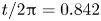 ${t}/{2{\rm \pi} } = 0.842$, (f)
  ${t}/{2{\rm \pi} } = 0.878$ and (g)
  ${t}/{2{\rm \pi} } = 0.943$.

Figure 23. Grid convergence for  $\epsilon =1.6$. There is a tendency to eject tiny droplets at the jet tip which makes it extremely challenging to measure jet asymptotes reliably. The insets represent the time instants when asymptotes are estimated and the boxed region in the main figures (b, c, d, e) provides the region which is depicted in the inset. Please refer to figure 17 in Appendix D for larger versions of the insets. (a)
 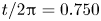 ${t}/{2{\rm \pi} } = 0.750$, (b)
  ${t}/{2{\rm \pi} } = 0.823$, (c)
  ${t}/{2{\rm \pi} } = 0.827$, (d)
 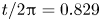 ${t}/{2{\rm \pi} } = 0.829$, (e)
 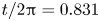 ${t}/{2{\rm \pi} } = 0.831$, (f)
  ${t}/{2{\rm \pi} } = 0.878$ and (g)
  ${t}/{2{\rm \pi} } = 0.943$.


 Open access