


1. Introduction
Turbulence in the natural environment is often generated under the influence of vertical shear of large-scale currents. The shear can cause Kelvin–Helmholtz instability, which makes a significant contribution to the transport of momentum and scalar in the flow (Smyth & Moum Reference Smyth and Moum2012). Shear flows with stable density stratification are commonly encountered in geophysical problems, such as the ocean mixing layer (Thorpe Reference Thorpe1978) and the atmospheric boundary layer (Mahrt Reference Mahrt1999). Therefore, turbulence under the influence of both shear and stable stratification has been studied by many researchers. One of the most simple examples of such turbulent flows is a stably stratified shear layer, which has been studied with both numerical simulations and laboratory experiments. Even under the stable stratification, the Kelvin–Helmholtz instability can produce turbulence when the shear is sufficiently strong (Strang & Fernando Reference Strang and Fernando2001). The Kelvin–Helmholtz billows can lead to secondary instabilities, which result in three-dimensional, fully developed turbulence (Klaassen & Peltier Reference Klaassen and Peltier1991). Once the fully developed turbulence is formed in the stably stratified shear layer, the turbulence begins to decay because of the viscous dissipation of turbulent kinetic energy under the stable stratification (Smyth & Moum Reference Smyth and Moum2000b; Pham & Sarkar Reference Pham and Sarkar2010). Visualization of the stably stratified shear layer showed that hairpin vortices and highly elongated structures with positive and negative velocity fluctuations appear after the turbulence decays significantly (Watanabe et al. Reference Watanabe, Riley, Nagata, Matsuda and Onishi2019a). These structures resemble turbulent structures found in wall turbulence. The hairpin vortices were also found in other stably stratified turbulence, e.g. turbulence arising from a breaking internal gravity wave (Fritts, Arendt & Andreassen Reference Fritts, Arendt and Andreassen1998) and turbulent Holmboe waves (Smyth & Winters Reference Smyth and Winters2003).
Three-dimensional direct numerical simulations (DNS) have been utilized to study the stably stratified shear layer. Direct numerical simulation studies often consider a temporally evolving, stably stratified shear layer with localized shear and stratification, where both velocity and density vary sharply across the layer. The flow develops with time in a computational domain that is periodic in the streamwise direction. This flow is often studied as an idealized problem of geophysical flows because a vertical profile of density in DNS resembles a density profile observed in turbulent patches in the ocean thermocline (Smyth & Moum Reference Smyth and Moum2000b). Direct numerical simulations of temporally evolving shear flows often have a problem in dealing with statistical convergence since the statistics are defined with spatial averages in homogeneous directions (Redford, Lund & Coleman Reference Redford, Lund and Coleman2015). The degree of statistical convergence depends on the size of the domain in homogeneous directions. Taking ensemble averages from different simulations also improves the convergence. However, because of the limited computational resource and the demand for simulating high-Reynolds-number flows, statistics are often calculated from a single run of DNS with a small domain (da Silva & Pereira Reference da Silva and Pereira2008; Kozul, Chung & Monty Reference Kozul, Chung and Monty2016; Watanabe, Zhang & Nagata Reference Watanabe, Zhang and Nagata2019b). Direct numerical simulations of temporally evolving, stratified shear layers have often been conducted with a computational domain which contains several Kelvin–Helmholtz billows (Smyth & Moum Reference Smyth and Moum2000b). Direct numerical simulations with such a small domain do not provide well-converged statistics, especially for high-order moments.
Another problem in DNS of temporally evolving turbulent flows is a confinement effect due to finite domain size. Recent DNS of a stratified shear layer with a very large domain found elongated large-scale structures (ELSS), whose streamwise length is much larger than the shear layer thickness (Watanabe et al. Reference Watanabe, Riley, Nagata, Matsuda and Onishi2019a). Most DNS studies in the existing literature could not observe the ELSS because of the limited size of the domain, where fluid motion at large scales is influenced by the boundary conditions. The interaction of fluid motions with different length scales, such as an energy transfer across the scales, is important in turbulent flows, and the confinement effect on large scales can also affect small-scale characteristics. Direct numerical simulations of stably stratified turbulence has been used to evaluate important parameters in oceanography, such as mixing efficiency and turbulent Prandtl number (Peltier & Caulfield Reference Peltier and Caulfield2003; Rahmani, Lawrence & Seymour Reference Rahmani, Lawrence and Seymour2014; Salehipour & Peltier Reference Salehipour and Peltier2015; Taylor et al. Reference Taylor, de Bruyn Kops, Caulfield and Linden2019). If the ELSS are dynamically important in the flow development, these findings based on DNS with a small domain can also be influenced by the confinement effects.
The typical large-scale structures in turbulent free shear flows have a length scale close to the transverse length of the flow, such as a momentum thickness of a turbulent mixing layer and a mean velocity halfwidth of a turbulent jet (Pope Reference Pope2000). In this paper turbulent motions at the transverse length scale of a turbulent shear flow are called large-scale motions (LSM). The LSM in turbulent free shear flows are often visualized as large-scale vortices (Bernal & Roshko Reference Bernal and Roshko1986; Taveira & da Silva Reference Taveira and da Silva2013). The wavenumber range corresponding to the shear layer thickness has a significant contribution to the turbulent kinetic energy in the stably stratified shear layer (Watanabe et al. Reference Watanabe, Riley, Nagata, Matsuda and Onishi2019a). Thus, the LSM also exists in the stably stratified shear layer. The ELSS can be distinguished from the LSM by the characteristic length because the ELSS grow much larger than the shear layer thickness. However, the LSM in the stably stratified shear layer is not clearly visible in flow visualization when the LSM coexists with the ELSS. Visualization of the LSM might require an adequate flow decomposition such as a proper orthogonal decomposition (Berkooz, Holmes & Lumley Reference Berkooz, Holmes and Lumley1993).
The purpose of this study is to investigate the statistical properties at large scales of the stably stratified shear layer with a special focus on LSM and ELSS. Although the ELSS in a stably stratified shear layer are found with flow visualization in Watanabe et al. (Reference Watanabe, Riley, Nagata, Matsuda and Onishi2019a), the dynamical properties of the ELSS are hardly known so far. It is of great interest to elucidate the generation mechanism of ELSS in turbulence research as similar structures also exist in wall turbulence (Nickels et al. Reference Nickels, Marusic, Hafez and Chong2005). The spectral energy budget is analysed in this study to identify the physical processes that contribute to the growth of the velocity and density fluctuations associated with the ELSS. This analysis will be useful to construct a physical model for the generation mechanism of the ELSS in future works. The statistical properties of LSM and ELSS are also investigated by spectral analysis. Since structures similar to the ELSS also exist in wall turbulence, the stably stratified shear layer is compared with turbulent boundary layers and channel flows. Furthermore, the scalings of energy spectra and second-order velocity structure functions at large scales are discussed based on the scalings in wall turbulence.
For this purpose, we perform a well-resolved large eddy simulation (LES) of a temporally evolving, stably stratified shear layer. The LES relies on an implicit subgrid scale (SGS) model, where a filtering scheme accounts for the dissipation at unresolved scales. This approach is often called implicit LES. It has been proved that implicit LES can accurately predict large-scale flow characteristics in various turbulent flows (Bogey & Bailly Reference Bogey and Bailly2009; Diamessis, Spedding & Domaradzki Reference Diamessis, Spedding and Domaradzki2011; Watanabe et al. Reference Watanabe, Zhang and Nagata2019b). Furthermore, the turbulent kinetic energy budget in implicit LES was shown to be consistent with DNS and experimental results (Bogey & Bailly Reference Bogey and Bailly2009; Watanabe et al. Reference Watanabe, Sakai, Nagata and Ito2016b). The LES conducted in this study is validated by comparison with DNS of the same flow. The low computational cost of LES enables us to repeatedly conduct the simulations for taking ensemble averages. Most statistics presented in this paper are difficult to accurately assess with a single run of DNS or LES because of insufficient statistical convergence. The methodologies of LES and DNS are described in § 2, where the energy budget equations in wavenumber space are also presented for velocity and density fluctuations in LES. Section 3 presents the results of LES, including the validation, the energy budgets and the scale dependence of statistics. Finally, the paper is summarized in § 4.
2. Implicit LES and DNS of a stably stratified shear layer
2.1. Temporally evolving, stably stratified shear layer
Implicit LES and DNS are performed for a temporally evolving, stably stratified shear layer with localized shear and stratification (figure 1), which has also been studied in the existing literature (Smyth & Moum Reference Smyth and Moum2000b; Mashayek & Peltier Reference Mashayek and Peltier2012; Watanabe, Riley & Nagata Reference Watanabe, Riley and Nagata2017). The Navier–Stokes equations with the Boussinesq approximation are used as the governing equations. The density field is expressed by  $\rho _{a}+\rho (x,y,z;t)$ with a constant reference density $\rho _{a}$ and the deviation from $\rho _{a}$ denoted by $\rho$. The flow is statistically homogeneous in the streamwise ( $x$) and spanwise ( $y$) directions, for which periodic boundary conditions are applied. The computational boundaries in the vertical ( $z$) direction are treated with the free-slip boundary conditions for velocity and with the zero-gradient condition in the boundary normal direction for density and pressure. The streamwise velocity and density differences across the stably stratified shear layer are denoted by $U_0$ and $\rho _0$ while $h_0$ is the initial layer thickness. Position $x_{i}$, time $t$, velocity $u_{i}$, pressure $p$ and density $\rho$ are non-dimensionalized as
 \begin{equation} x_{i}=\frac{\tilde{x}_{i}}{h_0};\quad t=\frac{\tilde{t}}{t_r};\quad u_{i}=\frac{\tilde{u}_{i}}{U_0};\quad p=\frac{\tilde{p}}{\rho_{a}U_0^2};\quad \rho=\frac{\tilde{\rho}}{\rho_0}. \end{equation}
Here,  $\tilde {f}$ denotes a variable $f$ with dimension and the reference time scale is defined as $t_r=h_{0}/U_0$. For convenience, $i=1,2$ and 3 represent the streamwise, spanwise and vertical components of vectors, where the velocity components in these directions are denoted by $u$,
$u$,  $v$ and $w$. The non-dimensionalized governing equations are written as
 $$\begin{gather} \frac{\partial u_{j}}{\partial x_{j}}=0, \end{gather}$$
 $$\begin{gather}\frac{\partial u_{i}}{\partial t}+\frac{\partial u_{i}u_{j}}{\partial x_{j}} ={-}\frac{\partial p}{\partial x_{i}} +\frac{1}{{Re}}\frac{\partial^{2} u_{i}}{\partial x_{j}\partial x_{j}}-Ri\rho\delta_{i3}, \end{gather}$$
 $$\begin{gather}\frac{\partial \rho}{\partial t} +\frac{\partial u_{j}\rho}{\partial x_{j}} =\frac{1}{RePr}\frac{\partial^{2} \rho}{\partial x_{j}\partial x_{j}}, \end{gather}$$
where successive indices imply summation. No external forcing is applied in the flow. The Reynolds number  ${Re}$, Richardson number $Ri$ and Prandtl number $Pr$ are defined as
 \begin{equation} {Re}=\frac{U_{0}h_{0}}{\nu};\quad Ri=\frac{g\rho_{0}h_{0}}{\rho_{a}U_{0}^2};\quad Pr=\frac{\nu}{\kappa}. \end{equation}
Here,  $\nu$ is the kinematic viscosity, $\kappa$ is the diffusivity coefficient for density, $g$ is the gravitational acceleration and $\delta _{ij}$ is the Kronecker delta. In previous studies, halves of the shear layer thickness ( $h_0/2$) and the velocity jump ( $U_0/2$) were also used to define the Reynolds number, which is written as $(h_0/2)(U_0/2)/\nu ={Re}/4$ (Salehipour & Peltier Reference Salehipour and Peltier2015). The Reynolds number used in this study should be multiplied by 1/4 for comparison with those studies.
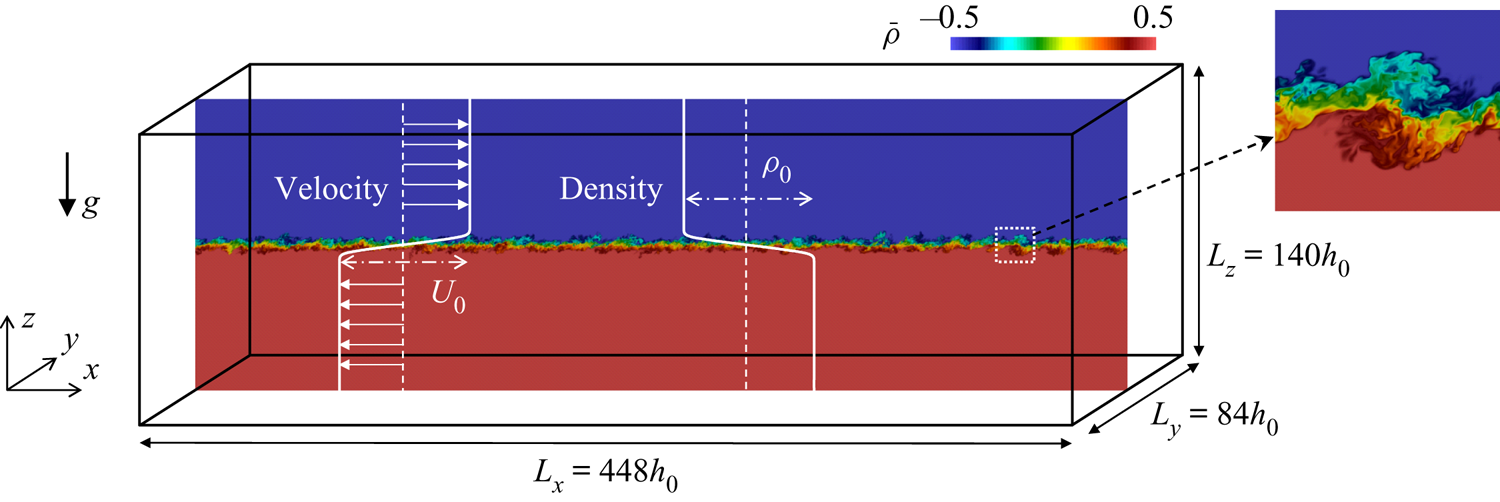
Figure 1. Schematic diagram of numerical simulations of a temporally evolving, stably stratified shear layer.
The flow is statistically homogeneous in the horizontal directions. Therefore, statistics are defined with an  $x$–
$x$– $y$ average. The average of a variable $f(x,y,z,t)$, $\langle f\rangle$, is obtained as a function of $(z,t)$,
 \begin{equation} \langle f\rangle(z,t)=\frac{1}{L_{x}L_{y}}\int_0^{L_y}\int_0^{L_x}f(x,y,z,t)\,\textrm{d}\kern0.06em x\,\textrm{d}y, \end{equation}
where  $L_x$ and $L_y$ are the sidelengths of the computational domain in the $x$ and $y$ directions. Ensemble averages of repeated simulations are also taken for improving the convergence. Fluctuations of $f$ from the average are denoted by $f'(x,y,z,t)=f(x,y,z,t)-\langle f\rangle (z,t)$, and the root-mean-square (r.m.s.) of the fluctuations is calculated as $f_{rms}(z,t)= (\langle f^2\rangle -\langle f\rangle ^2)^{1/2}$. In this study the energy spectra of velocity and density fluctuations are calculated with Fourier transform in the $x$ direction because the LSM and ELSS can be distinguished by their streamwise length scales. Fourier transform of $f(x,y,z,t)$ and its complex conjugate are denoted by $\hat {f}(k_x,y,z,t)$ and $\hat {f}^{*}(k_x,y,z,t)$, respectively, where $k_x$ is the streamwise wavenumber. An energy spectrum of velocity $u_{\alpha }$ is defined as $E_{u_{\alpha }}={{\rm Re}}[\langle \widehat {u_{\alpha }'}\widehat {u_{\alpha }'}^{*}\rangle ]$, where ${{\rm Re}}[\hat {f}]$ represents a real part of $\hat {f}$. Hereafter, Greek subscript letters indicate that no summation is taken over the subscripts. Similarly, a density spectrum is defined as $E_{\rho }(k_x,z,t)={{\rm Re}}[\langle \widehat {\rho '}\widehat {\rho '}^{*}\rangle ]$. Here, the spectra are evaluated with the average in the $y$ direction and the ensemble average of repeated simulations.
Following Smyth & Moum (Reference Smyth and Moum2000b), the initial profiles of density and mean streamwise velocity are given by
 $$\begin{gather} \tilde{\rho}={-}0.5\rho_{0}\tanh(2\tilde{z}/h_0), \end{gather}$$
 $$\begin{gather}\langle \tilde{u}\rangle = 0.5U_{0}\tanh(2\tilde{z}/h_{0}). \end{gather}$$
The mean velocity components in other directions are 0. The initial density field does not have any fluctuations. Artificial velocity fluctuations are superimposed to the mean velocity for  $|\tilde {z}|\leqslant h_0/2$ in order to trigger the turbulent transition of the shear layer. As explained below, DNS and LES are repeated with different initial velocity fluctuations to take ensemble averages. The fluctuations are generated with random numbers by the method described in Watanabe et al. (Reference Watanabe, Zhang and Nagata2019b). In this method, spatially correlated random velocity fluctuations are produced with a grid that discretizes the computational domain with a spacing of $\varDelta _{in}$. When three components of the velocity vector at each grid point are given by uniform random numbers, the characteristic length scale of velocity fluctuations is proportional to $\varDelta _{in}$ (Kempf, Klein & Janicka Reference Kempf, Klein and Janicka2005). Therefore, the length scale can be controlled by changing the non-dimensional grid size $\varDelta _{in}$, which is set as $\varDelta _{in}=0.35$. Velocity fluctuations in the $x$,
$x$,  $y$ and $z$ directions at each grid point are given by the uniform random numbers between $-1$ and 1. The fluctuations defined on this grid are interpolated onto the grid used in DNS or LES with trilinear interpolation. The velocity fluctuations are normalized such that the r.m.s. values normalized by $U_0$ are equal to $0.012$, which is small enough for the roller vortices of the Kelvin–Helmholtz instability to grow. If the initial velocity fluctuations are too strong, the roller vortices do not appear (Kaminski & Smyth Reference Kaminski and Smyth2019). Figure 2 shows the energy spectrum of initial streamwise velocity fluctuations, calculated with the Fourier transform in the $x$ direction. Here, $\lambda _x=2{\rm \pi} /k_x$ is the wavelength. Different lines are obtained from three sets of random numbers, which are generated by using a different random seed in a pseudorandom number generator. In this plot, the visible area under the curve of $k_xE_u$ represents the contribution to the velocity variance from a given wavelength (§ 3.3 provides further detailed explanations on the interpretation of the premultiplied spectrum). A peak of $k_xE_u$ is found at $\lambda _x\approx 1.2$, which is the energy-containing length scale of the initial fluctuations. The spectrum hardly varies among the three simulations, and the initial fluctuations are statistically identical among all repeated simulations.
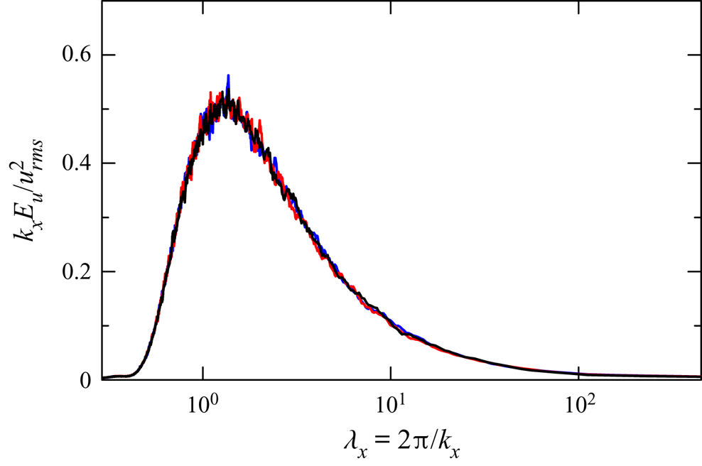
Figure 2. Premultiplied energy spectrum  $k_x E_u$ of initial streamwise velocity fluctuations in three simulations of run 2. The spectrum $E_u$ is calculated with Fourier transform in the $x$ direction, and is plotted against the wavelength $\lambda _x=2{\rm \pi} /k_x$. Here, $k_x E_u$ is normalized with the r.m.s. of velocity fluctuations $u_{rms}$.
2.2. Direct numerical simulation
The DNS code used in this study is based on a fractional step method with finite difference schemes. Variables are stored on a staggered grid, whose spacing is uniform in the horizontal direction and non-uniform in the vertical direction. Spatial derivatives are calculated with fully conservative finite difference schemes (Morinishi et al. Reference Morinishi, Lund, Vasilyev and Moin1998), where fourth-order and second-order schemes are used in the horizontal and vertical directions, respectively. The low-order schemes require more grid points to achieve the same effective spatial resolution as higher-order schemes. However, these low-order schemes have an advantage in the conservation properties. The fourth-order central difference applied on a uniform grid strictly conserves momentum and kinetic energy. The second-order scheme is also fully conservative even on a non-uniform grid, which is used in the vertical direction. On the other hand, higher-order schemes often violate the conservation laws. The same schemes are used in LES as explained below and these conservation properties are important in LES with a coarse grid. Time is advanced with a third-order Runge–Kutta method. The biconjugate gradient stabilized (Bi-CGSTAB) method is used to solve the Poisson equation for pressure. The same code was also used in our previous studies on turbulent shear flows (Watanabe et al. Reference Watanabe, Zhang and Nagata2019b), where the DNS results were compared well with experimental and other DNS studies.
2.3. Implicit LES
Large eddy simulation is performed with a coarse computational grid which is not fine enough to resolve fluctuations of all length scales existing in the flow. A variable  $f$ can be decomposed as $\bar {f}+f''$, where $\bar {f}$ is a grid-scale component that can be expressed on the LES grid while $f''$ is an SGS component. Large eddy simulation numerically solves governing equations for grid-scale components given by
 $$\begin{gather} \frac{\partial \bar{u}_{j}}{\partial x_{j}}=0, \end{gather}$$
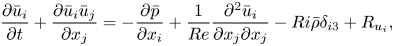 $$\begin{gather}\frac{\partial \bar{u}_{i}}{\partial t} +\frac{\partial \bar{u}_{i}\bar{u}_{j}}{\partial x_{j}} ={-}\frac{\partial \bar{p}}{\partial x_{i}} +\frac{1}{{Re}}\frac{\partial^{2}\bar{u}_{i}}{\partial x_{j}\partial x_{j}} -Ri\bar{\rho}\delta_{i3}+R_{u_i}, \end{gather}$$
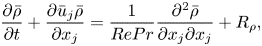 $$\begin{gather}\frac{\partial \bar{\rho}}{\partial t} +\frac{\partial\bar{u}_{j}\bar{\rho}}{\partial x_{j}} =\frac{1}{RePr}\frac{\partial^{2}\bar{\rho}}{\partial x_{j}\partial x_{j}}+R_{\rho}, \end{gather}$$
where  $R_{u_i}$ and $R_{\rho }$ are terms associated with the SGS. Here, the mathematical expressions of $R_{u_i}$ and $R_{\rho }$ are not required in the simulation as they are implicitly modelled in the implicit LES. In this study, $R_{u_i}$ and $R_{\rho }$ are approximated with a low-pass filter applied to $\bar {u}_{i}$ and $\bar {\rho }$, where the filter adds artificial dissipation of velocity and density fluctuations. The filter accounts for the dissipation in the SGS (Bogey & Bailly Reference Bogey and Bailly2009; Watanabe et al. Reference Watanabe, Sakai, Nagata and Ito2016b).
The LES code used in this study was developed based on the DNS code described above. The SGS terms are implicitly modelled with a tenth-order low-pass filter proposed in Kennedy & Carpenter (Reference Kennedy and Carpenter1994). The filter is applied to  $\bar {u}_{i}$ and $\bar {\rho }$ at the end of every computational time step. Numerical schemes except for the filter are the same as those used in the DNS. This LES code was also used for implicit LES of turbulent planar jets and turbulent boundary layers with a passive scalar transfer, where the code was validated by comparison with DNS and experiments (Tanaka, Watanabe & Nagata Reference Tanaka, Watanabe and Nagata2019; Watanabe et al. Reference Watanabe, Zhang and Nagata2019b).
For the post process of LES data, a filtering operator  $F$ is introduced by assuming that the low-pass filter used as the implicit SGS model changes a variable $f$ to $F(f)$. Then, the modelled SGS terms can be explicitly written as
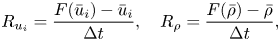 \begin{equation} R_{u_i}=\frac{F(\bar{u}_i)-\bar{u}_i}{\Delta t}, \quad R_{\rho}=\frac{F(\bar{\rho})-\bar{\rho}}{\Delta t}, \end{equation}
with a time increment  $\Delta t$ of the simulation. These expressions are useful to derive governing equations for various physical quantities, e.g. turbulent kinetic energy and scalar variance, in implicit LES (Bogey & Bailly Reference Bogey and Bailly2009; Tai, Watanabe & Nagata Reference Tai, Watanabe and Nagata2020). Equations (2.12a,b) are used for the analysis of the energy budgets of velocity and density fluctuations, where $F$ appears in the SGS dissipation terms.
2.4. Flow and computational parameters
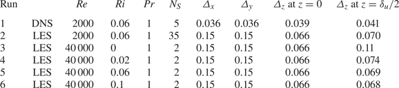
All DNS and LES are conducted with the domain size  $(L_{x}, L_{y}, L_{z})=(448, 84, 140)$. The number of grid points is $(N_{x}, N_{y}, N_{z})=(12\,288, 2304, 1200)$ in DNS and $(3072, 576, 700)$ in LES. Table 1 summarizes DNS and LES conducted in this study. The size of the computational domain is large enough for ELSS to grow (Watanabe et al. Reference Watanabe, Riley, Nagata, Matsuda and Onishi2019a). Both DNS and LES are performed for $({Re}, Ri, Pr)=(2000, 0.06, 1)$ (runs 1 and 2). Furthermore, LES is also performed for ${Re}=40\,000$ and $Pr=1$ with $Ri=0$, $0.02$, 0.06 and 0.1 (runs 3–6). For these ${Re}$ and $Ri$, the turbulent transition is caused by the Kelvin–Helmholtz instability. The same resolution is used for both ${Re}=2000$ and 40 000. This is because the length scale of large-scale fluctuations in the turbulent shear layer is related to $h_0$ rather than ${Re}$. A range of unresolved scales is wider for ${Re}=40\,000$ than for ${Re}=2000$ because the Kolmogorov scale becomes small as ${Re}$ increases. For $Ri=0$, the shear layer thickness monotonically increases with time. It is known that turbulence bounded by an irrotational flow induces large-scale velocity fluctuations outside the turbulent region (Taveira & da Silva Reference Taveira and da Silva2013; Watanabe, da Silva & Nagata Reference Watanabe, da Silva and Nagata2020) Therefore, velocity fluctuations are generated even far away from the turbulent shear layer. The very tall domain is used to prevent the confinement effects on the shear layer development and the velocity fluctuations outside the shear layer at $Ri=0$. Each simulation is repeated $N_S$ times by using different initial velocity fluctuations. Ensemble averages of statistics obtained in each simulation are taken for $N_S$ simulations. The flow is statistically symmetric with respect to $z$, and most statistics are presented for $z\geqslant 0$. Quantitative analyses with Fourier transform are presented for run 2 because many ensembles are required to obtain well-converged statistics of large-scale quantities. Runs 3–6 are used to examine $Ri$ dependence at high ${Re}$. Direct numerical simulation (run 1) is used to validate LES by comparison with run 2. Here, DNS reported in previous studies are not used for the validation because those DNS were conducted with a much smaller computational domain than the present simulations. Appendix A examines the confinement effects due to the finite domain size and shows that the computational domain used in previous studies can significantly affect the turbulent transition and the statistics of velocity and density.
Table 1. Parameters of DNS and LES. Grid sizes  $\varDelta _x$ and $\varDelta _y$ are constant while $\varDelta _{z}$ varies as a function of $z$. Table presents $\varDelta _{z}$ at $z=0$ and $\delta _u/2$, where $\delta _u$ is the shear layer thickness at $t=320$. The number of simulations repeated with different initial velocity fluctuations is denoted by $N_S$.
The time increment  $\Delta t$ is $0.02t_{r}$ in LES and $0.01t_r$ in DNS. The grid spacing is uniform in the streamwise and spanwise directions while the vertical location of the grid points is determined by
 \begin{equation} z(k)={-}\frac{L_{z}}{2\alpha_z} {\mathrm{atanh}} \left[\left({\mathrm{tanh}}\,\alpha_{z}\right) \left(1-2 \left(\frac{k-1}{N_z-1} \right) \right) \right], \end{equation}
with integers  $k=1,\ldots ,N_{z}$ and the grid stretching parameter $\alpha _z=3$, where atanh is an inverse hyperbolic tangent function. Equation (2.13) is used in this study because the grid size distribution is symmetric with respect to $z=0$ and the grid size increases with $|z|$. Compared with the DNS, the grid sizes in the LES are 4 times and 1.7 times larger in the horizontal and vertical directions, respectively. Table 1 presents the grid sizes $\varDelta _i$ in three directions, where $\varDelta _i$ is non-dimensionalized by $h_0$. Here, $\varDelta _{z}$ is taken at $z=0$ and at the edge of the shear layer $z=\delta _u/2$ at the end of the simulations ( $t=320$), where $\delta _u(t)$ is the shear layer thickness defined in § 3.2. The vertical distribution of $\varDelta _{z}$ for (2.13) can be found in Watanabe et al. (Reference Watanabe, Riley, Nagata, Onishi and Matsuda2018). The characteristic length of large-scale velocity fluctuations depends on time in the shear layer. At the beginning of the simulation, this length is the initial shear layer thickness $h_0$ because the initial roller vortices arising from the instability have a diameter with ${{O}}(h_0)$. After the turbulent transition, the vertical width of the turbulent shear layer, which is larger than $h_0$, characterizes large-scale fluctuations. Therefore, as long as the LES resolves $h_0$, the LES has a sufficient resolution to resolve the large-scale fluctuations even after the turbulent shear layer has fully developed. The number of grid points is determined so that $\varDelta _{i}\ll 1$ is satisfied. Although the LES grid resolves most length scales in run 2, the implicit SGS model is necessary because well-resolved LES without the SGS model results in an unphysical growth of energy at small scales, which affects the shape of energy spectra (Watanabe et al. Reference Watanabe, Zhang and Nagata2019b).
2.5. Spectral budget equations for turbulent kinetic energy and density variance in LES
The scale dependence of the budget of turbulent kinetic energy and density variance is studied with Fourier transform in the  $x$ direction. The governing equations for the energy spectra of velocity and density are presented for implicit LES in this section. Applying a Fourier transform to the equations for $\bar {u}_{\alpha }'$ yields the equations for $\widehat {\bar {u}_{\alpha }'}$. One can multiply the equations for $\widehat {\bar {u}_{\alpha }'}$ by $\widehat {\bar {u}_{\alpha }'}^{*}$ and take an average in order to derive the budget equations for $E_{u_{\alpha }}$ (Mizuno Reference Mizuno2016). The transport equation for $E_{u_{\alpha }}$ in implicit LES is written as
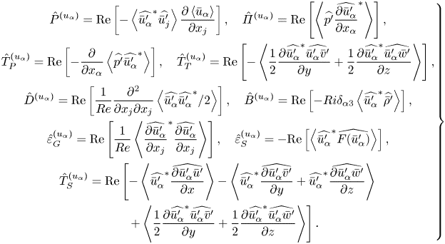
 \begin{align} \frac{\partial E_{u_{\alpha}}/2}{\partial t} +\langle \bar{u}_{j}\rangle \frac{\partial E_{u_{\alpha}}/2 }{\partial x_j} &=\hat{P}^{(u_{\alpha})} + \hat{\varPi}^{(u_{\alpha})} + \hat{T}_{P}^{(u_{\alpha})} + \hat{T}_{T}^{(u_{\alpha})}\nonumber\\ &\quad+ \hat{D}^{(u_{\alpha})} + \hat{T}_{S}^{(u_{\alpha})} + \hat{B}^{(u_{\alpha})} - \hat{\varepsilon}_{G}^{(u_{\alpha})} - \hat{\varepsilon}_{S}^{(u_{\alpha})} , \end{align}
with
 \begin{equation} \left.\begin{gathered}
\hat{P}^{(u_{\alpha})} = {{\rm Re}}\left[
-\left\langle\widehat{\bar{u}_{\alpha}'}^{*}\widehat{\bar{u}_{j}'}\right\rangle
\frac{\partial \left\langle
\bar{u}_{\alpha}\right\rangle}{\partial x_{j}}\right],
\quad \hat{\varPi}^{(u_{\alpha})} = {{\rm Re}}\left[
\left\langle \widehat{p'} \widehat{\frac{\partial
\bar{u}_{\alpha}'}{\partial x_{\alpha}}}^{*}
\right\rangle\right], \\ \hat{T}_{P}^{(u_{\alpha})} =
{{\rm Re}}\left[ - \frac{\partial}{\partial x_{\alpha}}
\left\langle \widehat{p'} \widehat{\bar{u}_{\alpha}'}^{*}
\right\rangle \right],\quad \hat{T}_{T}^{(u_{\alpha})} =
{{\rm Re}}\left[-\left\langle \frac{1}{2} \frac{\partial
\widehat{\bar{u}_{\alpha}'}^{*}
\widehat{\bar{u}_{\alpha}'\bar{v}'}}{\partial y}
+\frac{1}{2} \frac{\partial \widehat{\bar{u}_{\alpha}'}^{*}
\widehat{\bar{u}_{\alpha}'\bar{w}'}}{\partial
z}\right\rangle \right], \\ \hat{D}^{(u_{\alpha})} =
{{\rm Re}}\left[ \frac{1}{{Re}} \frac{\partial^{2}}{\partial
x_{j}\partial x_{j}} \left\langle
\widehat{\bar{u}_{\alpha}'}\widehat{\bar{u}_{\alpha}'}^{*}/2
\right\rangle \right],\quad \hat{B}^{(u_{\alpha})} =
{{\rm Re}}\left[{-}Ri\delta_{\alpha3}\left\langle\widehat{\bar{u}_{\alpha}'}^{*}\widehat{
\bar{\rho}'}\right\rangle\right], \\
\hat{\varepsilon}_{G}^{(u_{\alpha})} ={{\rm Re}}\left[
\frac{1}{{Re}} \left\langle \widehat{\frac{\partial
\bar{u}_{\alpha}'}{\partial x_{j}}}^{*}
\widehat{\frac{\partial \bar{u}_{\alpha}'}{\partial x_{j}}}
\right\rangle \right],\quad
\hat{\varepsilon}_{S}^{(u_{\alpha})} ={-}{{\rm Re}}\left[
\left\langle
\widehat{\bar{u}_{\alpha}'}^{*}\widehat{F(\bar{u}_{\alpha}')}\right\rangle
\right],\\ \hat{T}_{S}^{(u_{\alpha})} = {{\rm Re}}\left[
-\left\langle
\widehat{\bar{u}_{\alpha}'}^{*}\widehat{\frac{\partial
\bar{u}_{\alpha}'\bar{u}'}{\partial x}}\right\rangle
-\left\langle
\widehat{\bar{u}_{\alpha}'}^{*}\widehat{\frac{\partial
\bar{u}_{\alpha}'\bar{v}'}{\partial
y}}+\widehat{\bar{u}_{\alpha}'}^{*}\widehat{\frac{\partial
\bar{u}_{\alpha}'\bar{w}'}{\partial
z}}\right\rangle\right.\\ \quad \left.+\left\langle
\frac{1}{2} \frac{\partial \widehat{\bar{u}_{\alpha}'}^{*}
\widehat{\bar{u}_{\alpha}'\bar{v}'}}{\partial y}
+\frac{1}{2} \frac{\partial \widehat{\bar{u}_{\alpha}'}^{*}
\widehat{\bar{u}_{\alpha}'\bar{w}'}}{\partial
z}\right\rangle \right]. \end{gathered}\right\}
\end{equation}
\begin{equation} \left.\begin{gathered}
\hat{P}^{(u_{\alpha})} = {{\rm Re}}\left[
-\left\langle\widehat{\bar{u}_{\alpha}'}^{*}\widehat{\bar{u}_{j}'}\right\rangle
\frac{\partial \left\langle
\bar{u}_{\alpha}\right\rangle}{\partial x_{j}}\right],
\quad \hat{\varPi}^{(u_{\alpha})} = {{\rm Re}}\left[
\left\langle \widehat{p'} \widehat{\frac{\partial
\bar{u}_{\alpha}'}{\partial x_{\alpha}}}^{*}
\right\rangle\right], \\ \hat{T}_{P}^{(u_{\alpha})} =
{{\rm Re}}\left[ - \frac{\partial}{\partial x_{\alpha}}
\left\langle \widehat{p'} \widehat{\bar{u}_{\alpha}'}^{*}
\right\rangle \right],\quad \hat{T}_{T}^{(u_{\alpha})} =
{{\rm Re}}\left[-\left\langle \frac{1}{2} \frac{\partial
\widehat{\bar{u}_{\alpha}'}^{*}
\widehat{\bar{u}_{\alpha}'\bar{v}'}}{\partial y}
+\frac{1}{2} \frac{\partial \widehat{\bar{u}_{\alpha}'}^{*}
\widehat{\bar{u}_{\alpha}'\bar{w}'}}{\partial
z}\right\rangle \right], \\ \hat{D}^{(u_{\alpha})} =
{{\rm Re}}\left[ \frac{1}{{Re}} \frac{\partial^{2}}{\partial
x_{j}\partial x_{j}} \left\langle
\widehat{\bar{u}_{\alpha}'}\widehat{\bar{u}_{\alpha}'}^{*}/2
\right\rangle \right],\quad \hat{B}^{(u_{\alpha})} =
{{\rm Re}}\left[{-}Ri\delta_{\alpha3}\left\langle\widehat{\bar{u}_{\alpha}'}^{*}\widehat{
\bar{\rho}'}\right\rangle\right], \\
\hat{\varepsilon}_{G}^{(u_{\alpha})} ={{\rm Re}}\left[
\frac{1}{{Re}} \left\langle \widehat{\frac{\partial
\bar{u}_{\alpha}'}{\partial x_{j}}}^{*}
\widehat{\frac{\partial \bar{u}_{\alpha}'}{\partial x_{j}}}
\right\rangle \right],\quad
\hat{\varepsilon}_{S}^{(u_{\alpha})} ={-}{{\rm Re}}\left[
\left\langle
\widehat{\bar{u}_{\alpha}'}^{*}\widehat{F(\bar{u}_{\alpha}')}\right\rangle
\right],\\ \hat{T}_{S}^{(u_{\alpha})} = {{\rm Re}}\left[
-\left\langle
\widehat{\bar{u}_{\alpha}'}^{*}\widehat{\frac{\partial
\bar{u}_{\alpha}'\bar{u}'}{\partial x}}\right\rangle
-\left\langle
\widehat{\bar{u}_{\alpha}'}^{*}\widehat{\frac{\partial
\bar{u}_{\alpha}'\bar{v}'}{\partial
y}}+\widehat{\bar{u}_{\alpha}'}^{*}\widehat{\frac{\partial
\bar{u}_{\alpha}'\bar{w}'}{\partial
z}}\right\rangle\right.\\ \quad \left.+\left\langle
\frac{1}{2} \frac{\partial \widehat{\bar{u}_{\alpha}'}^{*}
\widehat{\bar{u}_{\alpha}'\bar{v}'}}{\partial y}
+\frac{1}{2} \frac{\partial \widehat{\bar{u}_{\alpha}'}^{*}
\widehat{\bar{u}_{\alpha}'\bar{w}'}}{\partial
z}\right\rangle \right]. \end{gathered}\right\}
\end{equation}
These terms are production  $\hat {P}^{(u_{\alpha })}$, pressure–strain correlation $\hat {\varPi }^{(u_{\alpha })}$, pressure diffusion $\hat {T}_{P}^{(u_{\alpha })}$, turbulent transport in physical space $\hat {T}_{T}^{(u_{\alpha })}$, viscous diffusion $\hat {D}^{(u_{\alpha })}$, buoyancy flux $\hat {B}^{(u_{\alpha })}$, viscous dissipation at the grid scales $\hat {\varepsilon }_{G}^{(u_{\alpha })}$, dissipation due to the implicit SGS model $\hat {\varepsilon }_{S}^{(u_{\alpha })}$ and turbulent transport in the wavenumber space $\hat {T}_{S}$. The advection term by mean velocity on the left-hand side of (2.14) is zero in the temporally evolving shear layer because $E_{u_{\alpha }}(k_x,z,t)$ does not depend on $x$ and $y$ and the mean velocity in the $z$ direction is zero. The pressure–strain correlation, $\hat {\varPi }^{(u_{\alpha })}$, is the redistribution term of the turbulent kinetic energy among three directions as $\hat {\varPi }^{(u)}+\hat {\varPi }^{(v)}+\hat {\varPi }^{(w)}=0$. The derivative $\partial /\partial x$ can be written as $ik_{x}$ in the wavenumber space. However, the derivative calculation in the wavenumber space is not consistent with the numerical schemes of the LES. Therefore, all spatial derivatives in these terms are calculated in the physical space.
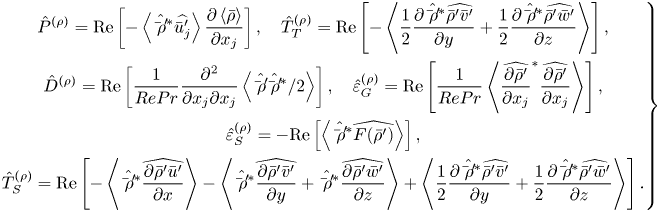
Similarly, we can derive the budget equation for the density spectrum  $E_{\rho }$,
 \begin{equation} \frac{\partial E_{\rho}/2}{\partial t} +\langle \bar{u}_{j}\rangle \frac{\partial E_{\rho}/2 }{\partial x_{j}} = \hat{P}^{(\rho)} + \hat{T}_{T}^{(\rho)} + \hat{D}^{(\rho)} + \hat{T}_{S}^{(\rho)} - \hat{\varepsilon}_{G}^{(\rho)} - \hat{\varepsilon}_{S}^{(\rho)} ,\end{equation}
with
 \begin{align} \left.\begin{gathered}
\hat{P}^{(\rho)} = {{\rm Re}}\left[ -\left\langle
\hat{\bar{\rho}'}^{*}\widehat{\bar{u}_{j}'}\right\rangle
\frac{\partial \left\langle
\bar{\rho}\right\rangle}{\partial x_{j}} \right],\quad
\hat{T}_{T}^{(\rho)} ={{\rm Re}}\left[ -\left\langle
\frac{1}{2} \frac{\partial
\hat{\bar{\rho}'}^{*}\widehat{\bar{\rho}'\bar{v}'}}{\partial
y} +\frac{1}{2} \frac{\partial
\hat{\bar{\rho}'}^{*}\widehat{\bar{\rho}'\bar{w}'}}{\partial
z} \right\rangle \right] ,\\ \hat{D}^{(\rho)} =
{{\rm Re}}\left[ \frac{1}{RePr} \frac{\partial^{2} }{\partial
x_{j}\partial x_{j}} \left\langle
\hat{\bar{\rho}'}\hat{\bar{\rho}'}^{*}/2\right\rangle
\right], \quad \hat{\varepsilon}_{G}^{(\rho)} =
{{\rm Re}}\left[ \frac{1}{RePr} \left\langle
\widehat{\frac{\partial \bar{\rho}'}{\partial x_{j}}}^{*}
\widehat{\frac{\partial \bar{\rho}'}{\partial x_{j}}}
\right\rangle \right], \\ \hat{\varepsilon}_{S}^{(\rho)}
={-}{{\rm Re}}\left[ \left\langle
\hat{\bar{\rho}'}^{*}\widehat{F(\bar{\rho}')}\right\rangle
\right],\\ \hat{T}_{S}^{(\rho)} = {{\rm Re}}\left[
-\left\langle \hat{\bar{\rho}'}^{*}\widehat{\frac{\partial
\bar{\rho}'\bar{u}'}{\partial x}}\right\rangle
-\left\langle \hat{\bar{\rho}'}^{*}\widehat{\frac{\partial
\bar{\rho}'\bar{v}'}{\partial
y}}+\hat{\bar{\rho}'}^{*}\widehat{\frac{\partial
\bar{\rho}'\bar{w}'}{\partial z}}\right\rangle
+\left\langle \frac{1}{2} \frac{\partial
\hat{\bar{\rho}'}^{*}\widehat{\bar{\rho}'\bar{v}'}}{\partial
y} +\frac{1}{2} \frac{\partial
\hat{\bar{\rho}'}^{*}\widehat{\bar{\rho}'\bar{w}'}}{\partial
z} \right\rangle \right] . \end{gathered}\right\}
\end{align}
\begin{align} \left.\begin{gathered}
\hat{P}^{(\rho)} = {{\rm Re}}\left[ -\left\langle
\hat{\bar{\rho}'}^{*}\widehat{\bar{u}_{j}'}\right\rangle
\frac{\partial \left\langle
\bar{\rho}\right\rangle}{\partial x_{j}} \right],\quad
\hat{T}_{T}^{(\rho)} ={{\rm Re}}\left[ -\left\langle
\frac{1}{2} \frac{\partial
\hat{\bar{\rho}'}^{*}\widehat{\bar{\rho}'\bar{v}'}}{\partial
y} +\frac{1}{2} \frac{\partial
\hat{\bar{\rho}'}^{*}\widehat{\bar{\rho}'\bar{w}'}}{\partial
z} \right\rangle \right] ,\\ \hat{D}^{(\rho)} =
{{\rm Re}}\left[ \frac{1}{RePr} \frac{\partial^{2} }{\partial
x_{j}\partial x_{j}} \left\langle
\hat{\bar{\rho}'}\hat{\bar{\rho}'}^{*}/2\right\rangle
\right], \quad \hat{\varepsilon}_{G}^{(\rho)} =
{{\rm Re}}\left[ \frac{1}{RePr} \left\langle
\widehat{\frac{\partial \bar{\rho}'}{\partial x_{j}}}^{*}
\widehat{\frac{\partial \bar{\rho}'}{\partial x_{j}}}
\right\rangle \right], \\ \hat{\varepsilon}_{S}^{(\rho)}
={-}{{\rm Re}}\left[ \left\langle
\hat{\bar{\rho}'}^{*}\widehat{F(\bar{\rho}')}\right\rangle
\right],\\ \hat{T}_{S}^{(\rho)} = {{\rm Re}}\left[
-\left\langle \hat{\bar{\rho}'}^{*}\widehat{\frac{\partial
\bar{\rho}'\bar{u}'}{\partial x}}\right\rangle
-\left\langle \hat{\bar{\rho}'}^{*}\widehat{\frac{\partial
\bar{\rho}'\bar{v}'}{\partial
y}}+\hat{\bar{\rho}'}^{*}\widehat{\frac{\partial
\bar{\rho}'\bar{w}'}{\partial z}}\right\rangle
+\left\langle \frac{1}{2} \frac{\partial
\hat{\bar{\rho}'}^{*}\widehat{\bar{\rho}'\bar{v}'}}{\partial
y} +\frac{1}{2} \frac{\partial
\hat{\bar{\rho}'}^{*}\widehat{\bar{\rho}'\bar{w}'}}{\partial
z} \right\rangle \right] . \end{gathered}\right\}
\end{align}
These terms represent production  $\hat {P}^{(\rho )}$, turbulent transport in physical space $\hat {T}_{T}^{(\rho )}$, diffusion $\hat {D}^{(\rho )}$, dissipation at the grid scales $\hat {\varepsilon }_{G}^{(\rho )}$, dissipation due to the implicit SGS model $\hat {\varepsilon }_{S}^{(\rho )}$ and turbulent transport in the wavenumber space $\hat {T}_{S}^{(\rho )}$.
3. Results and discussion
3.1. Flow visualization
Figure 3 shows an instantaneous density profile on an  $x$–
$x$– $z$ plane at $t=60$ and 200 in run 2. Vortices generated by the Kelvin–Helmholtz instability can be seen in figure 3(a). After these vortices collapse, the flow becomes turbulent with small-scale density fluctuations in figure 3(b). This temporal development of the stably stratified shear layer agrees well with the previous DNS with the same Reynolds number and Richardson number (Watanabe et al. Reference Watanabe, Riley, Nagata, Matsuda and Onishi2019a).
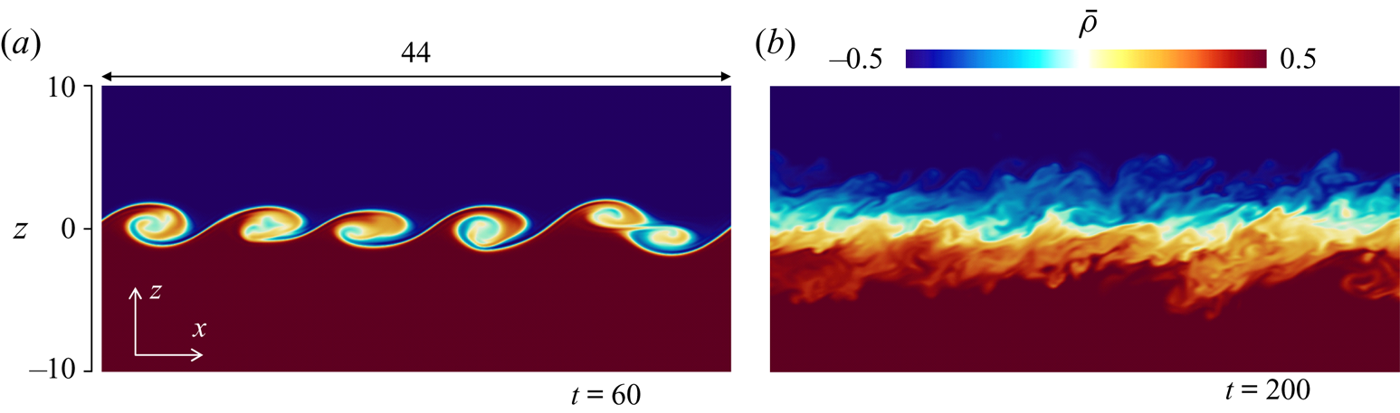
Figure 3. Density  $\bar {\rho }$ on an $x$–
$x$– $z$ plane at (a) $t=60$ and (b) $t=200$ in run 2. Only a small part of the computational domain is shown here.
Figure 4 visualizes streamwise velocity fluctuations  $\bar {u}'$ in run 2 on the horizontal plane at $z=0$ from $t=2$ to 320. The characteristic length scale of the velocity fluctuations increases with time. At late time, the velocity distribution is highly anisotropic, and regions with positive and negative $\bar {u}'$ are elongated in the $x$ direction. These are related to the ELSS, which were also found in previous DNS (Watanabe et al. Reference Watanabe, Riley, Nagata, Matsuda and Onishi2019a). Figure 4(f) depicts the length of the shear layer thickness $\delta _u$, which is defined with the mean streamwise velocity $\langle \bar {u}\rangle$ as the vertical distance between $\langle \bar {u}\rangle =-0.49$ and 0.49. The vertical profile of $\langle \bar {u}\rangle$ is presented in the next subsection. The streamwise length of the ELSS is as large as $10\delta _u$ while the spanwise length is about $\delta _u$. The streamwise and spanwise sizes of the ELSS are smaller than $L_x$ and $L_y$ even at $t=320$, respectively, and the computational domain contains multiple ELSS identified by $\bar {u}'$. The longitudinal auto-correlation functions of $u$ and $v$ are defined as
 $$\begin{gather} f_u(r_x,z,t)=\langle u'(x,y,z,t)u'(x+r_x,y,z,t)\rangle / u_{rms}^2(z,t), \end{gather}$$
 $$\begin{gather}f_v(r_y,z,t)=\langle v'(x,y,z,t)v'(x,y+r_y,z,t)\rangle / v_{rms}^2(z,t). \end{gather}$$
Here,  $r_i$ is the distance between two points separated in the $i$ direction. If the domain is small compared with the length scale of the flow, $f_u$ and $f_v$ do not reach zero at large scales because the periodic boundary conditions generate artificial correlation between two points (Davidson Reference Davidson2004). In run 2, $f_u(r_x)$ and $f_v(r_y)$ at $z=0$ and $t=320$ reach 0 at $r_x=41.1$ and $r_y=8.2$, which are about $L_x/10$ and $L_y/10$, respectively. Thus, the domain is large enough to prevent the finite domain size from affecting the development of turbulence. Velocity fluctuations at $t=2$ are related to the initial velocity fluctuations. The roller vortices of the Kelvin–Helmholtz instability exist at $t=60$. The diameter of the roller vortices at $t=60$ is ${{O}}(h_0)$ in figure 3(a), and this length is much smaller than the streamwise length of the ELSS, which is as large as $10^2h_0$. Thus, the velocity fluctuations after $t=120$ are hardly correlated with those at $t=2$ and 60.
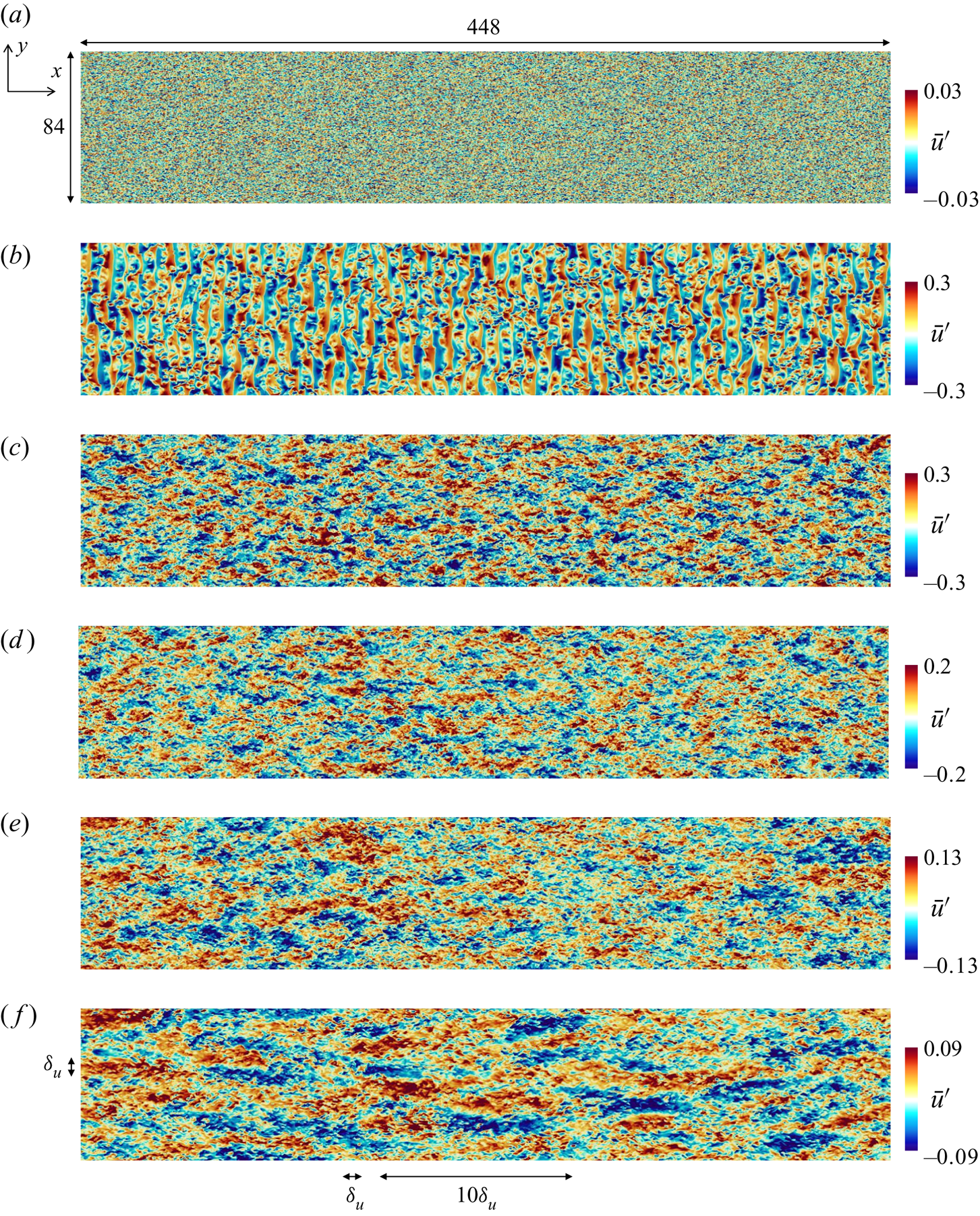
Figure 4. Streamwise velocity fluctuations  $\bar {u}'$ on the horizontal plane at the centre of the shear layer in run 2: (a) $t =2$; (b) $t =60$; (c) $t =120$; (d) $t =180$; (e) $t =240$; (f) $t =320$. Figure (f) depicts the size of $\delta _u$ and $10\delta _u$, where $\delta _u$ is the shear layer thickness defined with the mean velocity profile.
3.2. Fundamental statistics of stably stratified shear layers
The LES is validated by comparison between runs 1 (DNS) and 2 (LES). Figure 5(a) compares vertical profiles of mean streamwise velocity and density. These profiles show that the shear layer grows from  $t=100$ to 240 because both mean streamwise velocity (momentum) and density are transferred in the vertical direction by turbulence. Figure 5(b) shows the temporal evolution of r.m.s. velocity fluctuations at $z=0$ and shear layer thickness $\delta _u$. The figure also includes $u_{rms}$ in five LES before the ensemble average is taken. The difference among the five simulations is small, and the domain size is large enough to obtain well-converged statistics for r.m.s. quantities. When the turbulence is generated by the instability, the r.m.s. velocity fluctuations increase with time. The fluctuations begin to decay after they reach a peak. The shear layer thickness also increases at early time. However, the growth of the shear layer thickness becomes slow after $t\approx 150$ because of the stable stratification. These statistics are almost identical between the LES and DNS.
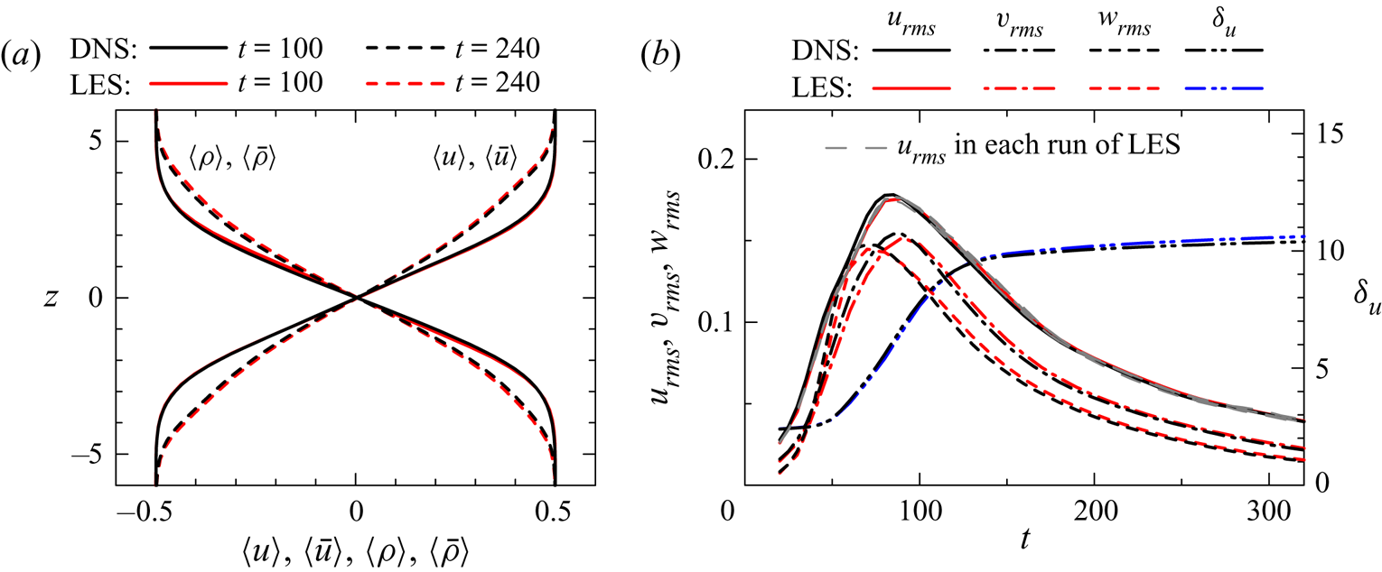
Figure 5. Comparisons between DNS (run 1) and LES (run 2). (a) Vertical profiles of mean velocity and density at  $t=100$ and 240. (b) Temporal variations of root-mean-squared velocity fluctuations at $z=0$ and shear layer thickness $\delta _u$. Grey broken lines represent $u_{rms}$ in five simulations of LES.
Figure 6(a) compares the energy spectrum of streamwise velocity,  $E_u$, between runs 1 and 2. The LES and DNS results agree well with each other for a low wavenumber range while $E_u$ in the LES sharply drops for $k_x\gtrsim 10$. The spectrum at $t=60$ has a peak at $k_x\approx 0.6$, which is associated with the roller vortices. The wavelength of this peak is $\lambda _x\approx 10$, which is much smaller than the streamwise length of the ELSS at $t=320$. Therefore, the length scales of large-scale fluctuations are different between the transitional and fully developed states. As also found in figure 4, the velocity fluctuations during the transition are not directly related to those at late time. The figure also shows $E_u$ obtained in each run of the LES. The shape of $E_u$ at $t=60$ is qualitatively similar among nine simulations, and the size and spacing of the roller vortices are statistically identical among all simulations. Quantitative variations among different simulations are noticeable for a low wavenumber range, for which the convergence of spectra is improved by taking ensemble averages of 35 simulations.
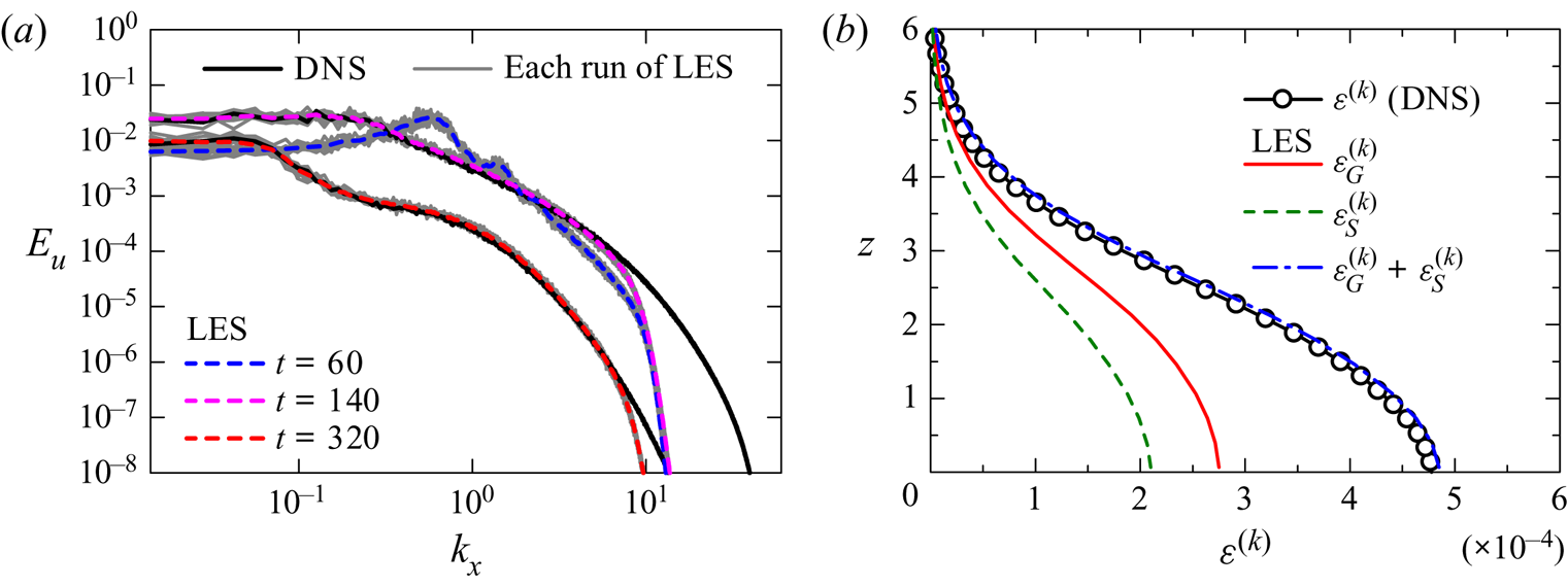
Figure 6. (a) Energy spectrum of streamwise velocity  $E_u$ at the centre of the shear layer at $t=60$, 140 and 320 in LES (run 2). Direct numerical simulation results at $t=140$ and 320 are also shown for comparison. Grey lines are $E_u$ in each simulation of LES (nine simulations). (b) Vertical profiles of turbulent kinetic energy dissipation rate at $t=140$ in DNS ( $\varepsilon ^{(k)}$ in run 1) and LES ( $\varepsilon _{G}^{(k)}+\varepsilon _{S}^{(k)}$ in run 2). The dissipation terms of grid scales ( $\varepsilon _{G}^{(k)}$) and subgrid scales ( $\varepsilon _{S}^{(k)}$) are also shown in the figure.
In implicit LES the dissipation terms of turbulent kinetic energy by the grid scales and the SGS model are given respectively by
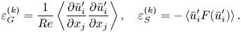 \begin{equation} \varepsilon_{G}^{(k)}=\frac{1}{{Re}} \left\langle\frac{\partial \bar{u}_{i}'}{\partial x_{j}}\frac{\partial \bar{u}_{i}'}{\partial x_{j}}\right\rangle, \quad \varepsilon_{S}^{(k)}={-}\left\langle \bar{u}_{i}'F(\bar{u}_{i}')\right\rangle. \end{equation}
Figure 6(b) shows the turbulent kinetic energy dissipation rate at  $t=140$ in runs 1 and 2. The total dissipation rate $\varepsilon _{G}^{(k)}+\varepsilon _{S}^{(k)}$ in the LES agrees well with the dissipation rate in the DNS, which is calculated as $\varepsilon ^{(k)}=\varepsilon _{G}^{(k)}$ by replacing $\bar {u}_{i}'$ with $u_i'$ in (3.3a,b). Therefore, the amount of dissipation is accurately controlled by the implicit SGS model. In the LES, $\varepsilon _{S}^{(k)}$ is as large as $\varepsilon _{G}^{(k)}$, and about one half of the energy dissipation is treated with the model at $t=140$. The implicit LES does not use the dynamic adjustment of the filter. The averaged energy dissipation rate in turbulence is generally controlled by the averaged interscale energy flux from large to small scales. The filter dissipates the energy at resolved small scales before the energy is transferred to further small scales. The good agreement in the dissipation rate between LES and DNS may be explained by the spatial resolution of LES, which is good enough to resolve large-scale fluctuations that determine the averaged interscale energy flux.
Figure 7(a) shows the temporal evolution of  $\delta _u$ at ${Re}=40\,000$ in runs 3–6. In the non-stratified turbulent shear layer ( $Ri=0$), $\delta _u$ almost linearly increases with time for $t\gtrsim 100$. As also found at ${Re}=2000$, the growth of $\delta _u$ at ${Re}=40\,000$ is very slow for $t\gtrsim 150$ at $Ri=0.06$ and 0.1. However, $\delta _u$ at $Ri=0.02$ gradually increases even for $t\gtrsim 150$. Figure 7(b) shows $u_{rms}$ on the shear layer centreline at ${Re}=40\,000$. In a self-similar turbulent mixing layer, $u_{rms}$ at $z=0$ does not vary with time (Rogers & Moser Reference Rogers and Moser1994). Indeed, $u_{rms}\approx 0.17$ at $Ri=0$ hardly varies after the turbulent shear layer has fully developed, and this value of 0.17 agrees well with previous studies on self-similar turbulent mixing layers (Rogers & Moser Reference Rogers and Moser1994). The time of the peak in $u_{rms}$ depends on $Ri$. Furthermore, comparison of $u_{rms}$ between figures 5(b) and 7(b) also confirms that $u_{rms}$ at $Ri=0.06$ reaches a peak slightly earlier for ${Re}=40\,000$ than for ${Re}=2000$. These differences in the initial growth of $u_{rms}$ imply that the detailed transition process depends on ${Re}$ and $Ri$.
$Ri$.
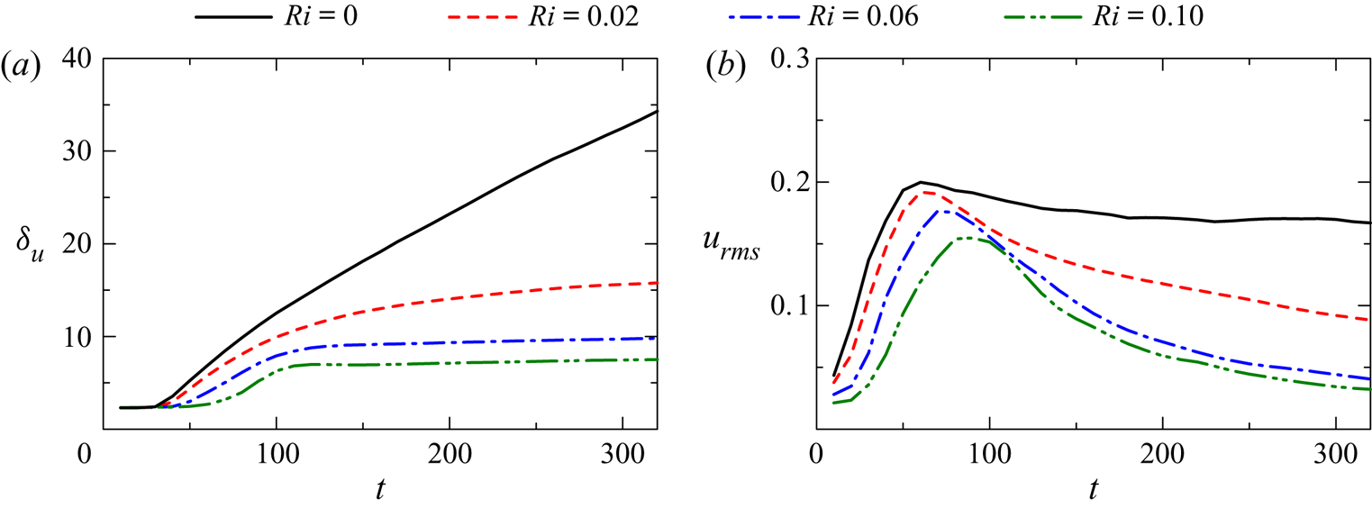
Figure 7. Temporal variations of (a) shear layer thickness  $\delta _u$ and (b) r.m.s. streamwise velocity fluctuations at $z=0$ for ${Re}=40\,000$ (runs 3–6).
The comparisons between the DNS and LES confirm that the LES accurately captures large-scale velocity and density fluctuations of the flow. The LES results will be used to assess the statistical properties of the stably stratified shear layer. In the rest of the paper most results are presented for  $t=140$, 240 and 320. Table 2 summarizes important parameters of the flow obtained by LES at these time instances, where $L_O=\sqrt {\varepsilon ^{(k)}/N^3}$ is the Ozmidov scale defined with the buoyancy frequency $\tilde {N}=\sqrt {-(g/\rho _a) \langle \partial \tilde {\rho }/\partial \tilde {z} \rangle }$ $(N=\tilde {N}t_r)$, $\eta =({Re}^{3}\varepsilon ^{(k)})^{-1/4}$ is the Kolmogorov scale, ${Re}_b=(L_O/\eta )^{4/3}$ is the buoyancy Reynolds number and $Ri_g=N^2/\langle \partial u /\partial z\rangle ^{2}$ is the gradient Richardson number. The turbulent kinetic energy dissipation rate in LES is calculated as $\varepsilon ^{(k)}=\varepsilon _{G}^{(k)}+\varepsilon _{S}^{(k)}$. The table shows $L_{O}$, $\eta$, ${Re}_b$ and $Ri_g$ obtained at $z=0$. Here, $L_{O}$ and $\eta$ are normalized by $\delta _u$ because the energy spectra will be presented as functions of a wavelength normalized by $\delta _u$. In the rest of the paper, $z$ is also normalized by $\delta _u$ because $z/\delta _u$ is useful to indicate the location with respect to the shear layer thickness. In run 2 the spatial resolution $\varDelta _x$ is $2.2\eta$- $8.0\eta$, where $\varDelta _x/\eta$ decreases with time. Thus, most length scales are resolved in run 2, which will be used to evaluate the transport equations of energy spectra. Runs 3–6 have $\varDelta _x/\eta ={{O}}(10^1)$ and large-scale velocity and density fluctuations are well resolved in LES. The Ozmidov scale is often interpreted as the smallest length scale that is affected by the buoyancy, and it is considered that vertical turbulent motions at scales greater than $L_O$ are significantly damped. The buoyancy Reynolds number is defined as the ratio between $L_O$ and $\eta$. As $\eta$ represents the smallest scale of turbulence, ${Re}_b\gg 1$ indicates that small-scale turbulent motions are not directly influenced by the stable stratification. This is comfortably the case at $t=140$ with ${Re}_b=93$ for $({Re},Ri)=(2000,0.06)$. However, smaller values of ${Re}_b$ at the later time indicate that turbulent motions at the smallest scale are strongly suppressed by the buoyancy. At ${Re}=40\,000$, ${Re}_b$ is larger than ${{O}}(10^1)$ except at late time with $Ri=0.1$. At $Ri=0.06$ and 0.1, $Ri_g=0.42 - 0.56$ weakly depends on time after $t=140$. On the other hand, $Ri_g$ increases from 0.16 to 0.24 at $({Re}, Ri)=(40\,000, 0.02)$ because the shear layer thickness also grows with time.
Table 2. Statistical properties of the stably stratified shear layer in LES. Values of  $L_{O}$, $\eta$, ${Re}_b$ and $Ri_g$ are taken at the centre of the shear layers.
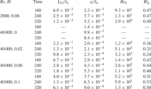
3.3. Energy spectra of velocity and density
The energy spectra of velocity and density fluctuations are calculated with Fourier transform in the  $x$ direction. These spectra, premultiplied by the streamwise wavenumber $k_x$, are plotted against the vertical location $z$ and the streamwise wavelength $\lambda _x=2{\rm \pi} /k_x$, where $\lambda _x$ is shown on a logarithmic scale. When $E_u(k_x)$ at a given vertical position is shown in a linear plot, the visible area beneath the curve between wavenumbers $k_{x1}$ and $k_{x2}$ can be interpreted as the contribution to $\langle u'^2\rangle$ from $k_{x1}\leqslant k_{x}\leqslant k_{x2}$ because of $\langle u'^2\rangle =\int _0^{\infty } E_u(k_x)\,\textrm {d}k_x$. The equivalent relation for the logarithmic coordinate of $k_{x}$ is $\langle u'^2\rangle =\int _{-\infty }^{\infty } k_{x}E_ud(\log _{10}{k_x})$, which is obtained with $dk_x=k_xd(\log _{10}{k_x})$. Therefore, when the spectrum is plotted on the logarithmic coordinate of $k_x$, $k_xE_u$ is useful because it is the contribution to $\langle u'^2\rangle$ on the coordinate of $\log _{10}{k_x}$. This meaning of the premultiplied spectrum is held even if $\lambda _x=2{\rm \pi} /k_x$ is used instead of $k_x$ because $d\log _{10}{k_x}$ is proportional to $-d\log _{10}{\lambda _x}$. As the turbulent kinetic energy is distributed over a wide range of scales, the premultiplied spectrum is widely used to assess the scale dependence of turbulent kinetic energy (Kim & Adrian Reference Kim and Adrian1999; Hutchins & Marusic Reference Hutchins and Marusic2007; Takamure et al. Reference Takamure, Ito, Sakai, Iwano and Hayase2018). Similarly, premultiplied cospectra related to turbulent fluxes of momentum and density have been used in previous studies on stratified turbulent flows (Lienhard & van Atta Reference Lienhard and van Atta1990; Gerz & Schumann Reference Gerz and Schumann1996; Komori & Nagata Reference Komori and Nagata1996).
Figure 8(a–c) shows the energy spectrum of streamwise velocity,  $k_{x}E_u$, at $t=140$, 240 and 320 in run 2. As also observed in previous DNS (Watanabe et al. Reference Watanabe, Riley, Nagata, Matsuda and Onishi2019a), the spectral shape significantly changes with time. At $t=140$, $k_{x}E_{u}$ at each vertical location has a single peak around $\lambda _x/\delta _u\approx 2$. At late time, the middle of the shear layer has a spectral shape with two peaks at $\lambda _x/\delta _u\approx 1$ and 10 while a single peak can be identified for $z/\delta _u\gtrsim 0.3$. The peak in $k_{x}E_{u}$ at $\lambda _x/\delta _u \approx 10$ is related to the ELSS visualized in figure 4(f), where regions with positive and negative fluctuations extend over about $10\delta _u$ in the $x$ direction. A similar spectral evolution can be found for $E_v$ and $E_w$ shown in figure 8(d–i). Figure 8(j-l) shows $k_{x}E_{\rho }$ at the same time instances. As found for the kinetic energy spectra, $k_{x}E_{\rho }$ in the middle of the shear layer at $t=320$ has two peaks at $\lambda _x/\delta _u \approx 0.6$ and $8$. However, $k_{x}E_{\rho }$ decreases with $z$ while the velocity spectra have a large peak at $z/\delta _u\approx 0.4$. These spectral shapes in the LES generally agree with the DNS results in Watanabe et al. (Reference Watanabe, Riley, Nagata, Matsuda and Onishi2019a). However, the peak locations are more clearly identified in the LES since ensemble averages are taken in this study.
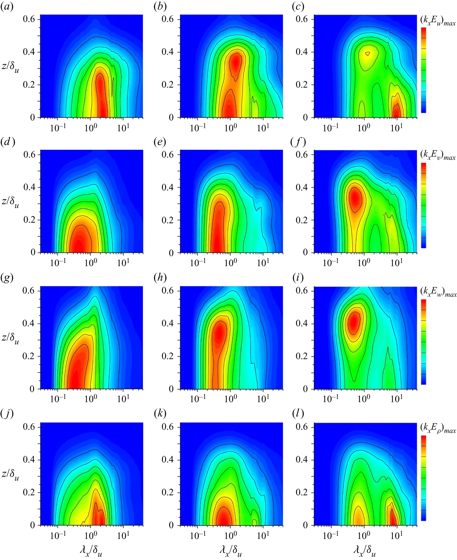
Figure 8. Premultiplied energy spectra of velocity and density,  $k_{x}E_{\alpha }$ ( $\alpha =u, v, w$ or $\rho$) in run 2 ( ${Re}=2000$, $Ri=0.06$), plotted against the streamwise wavelength $\lambda _x=2{\rm \pi} /k_x$ and the vertical location $z$: (a,d,g,j) $t=140$; (b,e,h,k) $t=240$; (c,f,i,l) $t=320$. (a–c) Streamwise velocity $E_u$; (d–f) spanwise velocity $E_v$; (g–i) vertical velocity $E_w$; (j–l) density $E_\rho$. The colour contours are normalized by the peak values at specific times.
The double-peak spectra at late time indicate that the flow in the middle of the shear layer has two energy-containing length scales, which can be identified as the peak wavelengths. One is the short peak-wavelength of the spectra, which is close to the shear layer thickness  $\delta _u$. In turbulent free shear flows, such as jets, wakes and mixing layers, a characteristic length of LSM is the width of the flow (Pope Reference Pope2000). Therefore, the peak at $\lambda _x\sim \delta _u$ is associated with usual LSM, which appear in a turbulent shear layer even without stable stratification. Fluid motions at this length scale are simply referred to as ‘LSM’. The other energy-containing length scale is obtained as the long peak-wavelength, which is much larger than $\delta _u$. This length scale is related to the streamwise length of elongated patterns of velocity fluctuations visualized in figure 4(f). Therefore, fluid motions associated with fluctuations at the long peak-wavelength are called ‘ELSS’.
The peak in  $k_{x}E_{u}$ associated with the ELSS is found only for $|z|/\delta _u \lesssim 0.3$. The ELSS hardly reach the interfacial region between the turbulent shear layer and the non-turbulent region, which are separated by a thin interfacial layer (turbulent/non-turbulent interface). Visualization of the turbulent/non-turbulent interface in a stably stratified shear layer showed that the interface geometry does not exhibit an imprint of the ELSS (Watanabe, Riley & Nagata Reference Watanabe, Riley and Nagata2016a). This is because the ELSS appear in the middle of the shear layer while the interface is formed at the outer edge of the shear layer. The ELSS and the interface are separated in space, and it is expected that the ELSS do not have significant influences on the turbulent/non-turbulent interface.
The existence of LSM and ELSS for  ${Re}<2000$ was reported in Watanabe et al. (Reference Watanabe, Riley, Nagata, Matsuda and Onishi2019a). Runs 3–6 are used to examine them at high ${Re}$. Figure 9 shows $k_x E_{u}$ at $z=0$ for ${Re}=40\,000$. The spectrum $k_x E_{u}$ is normalized by its maximum value $[k_x E_{u}]_{max}$ at $z=0$ in order to compare the plots at different time. The formation of the double-peak spectrum occurs for $Ri=0.06$ and 0.1. For low $Ri$,
$Ri$,  $k_x E_{u}$ has a single peak and the flow has only one characteristic length scale at large scales. This large single peak is expected from the presence of large-scale roller vortices in a turbulent mixing layer without density stratification (Balaras, Piomelli & Wallace Reference Balaras, Piomelli and Wallace2001). The peak wavelength at $Ri=0$ and 0.02 is about $\lambda _x/\delta _u=2 - 3$, which is much smaller than the size of ELSS. The ELSS corresponding to the spectral peak at $\lambda _x/\delta _u\approx 10^{1}$ appear only at moderately large $Ri$. This peak at $\lambda _x/\delta _u\approx 10^{1}$ appears earlier at $Ri=0.1$ than at $Ri=0.06$. Thus, the ELSS develop faster for higher $Ri$.
$Ri$.
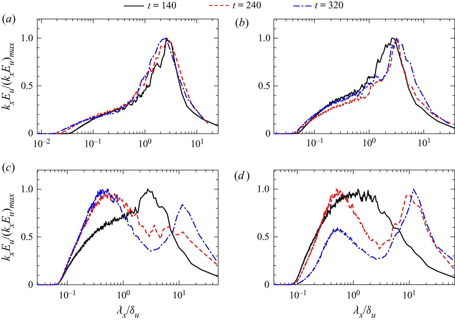
Figure 9. Energy spectra of streamwise velocity at  $z=0$ at $t=140, 240$ and 320 in runs 3–6 $({Re}=40\,000)$: (a) $Ri=0$ (run 3); (b) $Ri=0.02$ (run 4); (c) $Ri=0.06$ (run 5); (d) $Ri=0.1$ (run 6). For comparison of the spectra at different $t$,
$t$,  $k_x E_{u}$ is normalized by its maximum value $[k_x E_{u}]_{max}$ at each time instance.
3.4. Characteristics of large-scale velocity and density fluctuations
The scale dependence of turbulent statistics is investigated with the energy spectra in run 2. The characteristic length scales of LSM and ELSS are estimated with the spectral peaks. Figure 10(a) shows the turbulent kinetic energy spectrum  $E_{k}=(E_u+E_v+E_w)/2$ and density spectrum $E_\rho$ at $t=260$ on the centreline, where two peaks can be identified for both spectra. Here, the short peak-wavelength of $E_{\rho }$ is denoted by $\varLambda _{S\rho }$ while the long peak-wavelength is denoted by $\varLambda _{L\rho }$. Similarly, $\varLambda _{Sk}$ and $\varLambda _{Lk}$ represent the short and long peak-wavelengths of $E_k$, respectively. The premultiplied spectra at $z=0$ are plotted on the discrete coordinate of $\lambda _x$, where one can find the peaks in $E_{k}$ and $E_\rho$. A third-order polynomial curve fitting with five discrete points centred at the peak of $E_k$ or $E_\rho$ is applied to determine the peak wavelength from the fitted curve. These peak wavelengths are the characteristic length scales of LSM and ELSS. The spectra before $t=220$ have only a single peak at $z=0$ and the ELSS have not formed yet. Figure 10(b) shows temporal variations of the peak wavelengths obtained at $z=0$ after $t=220$. Here, these wavelengths are normalized by $\delta _u$, which hardly increases with time for $t\geqslant 220$ as shown in figure 5(b). The short peak-wavelength weakly depends on time: $\varLambda _{S\rho }$ and $\varLambda _{Sk}$ stay between $0.5\delta _u$ and $0.7\delta _u$. On the other hand, the long peak-wavelengths increase with time approximately from $5\delta _u$ to $9\delta _u$. Therefore, the length scale of LSM hardly grows with time while the length of ELSS monotonically increases. The increase of $\varLambda _{Lk}$ and $\varLambda _{L\rho }$ can be caused by the deformation due to mean shear. In the stratified shear layer a time scale of turbulence increases as the turbulence decays, while a time scale of the mean shear $\sim U_0/\delta _u$ is almost independent of time because $\delta _u$ hardly changes with time once the stably stratified turbulent shear layer has fully developed. Therefore, the turbulence time scale becomes much longer than the shear time scale at late time. In the stably stratified shear layer investigated in this study, the integral shear parameter defined as a turbulence-to-shear time scale ratio exceeds 15 (Watanabe et al. Reference Watanabe, Riley, Nagata, Matsuda and Onishi2019a), which is larger than typical values of 3–6 in non-stratified turbulent free shear flows (Pope Reference Pope2000). In general, turbulence with larger scales evolves more slowly. Therefore, the turbulent motions, especially at scales of the ELSS, evolve much more slowly than the shear time scale, and its evolution is possibly approximated by rapid distortion theory (Savill Reference Savill1987). The theory predicts that the longitudinal integral length scale in the mean flow direction monotonically increases with time in turbulence with a simple shear (Lee, Kim & Moin Reference Lee, Kim and Moin1990). This behaviour is consistent with the growth of $\varLambda _{Lk}$ and $\varLambda _{L\rho }$ found in figure 10(b).
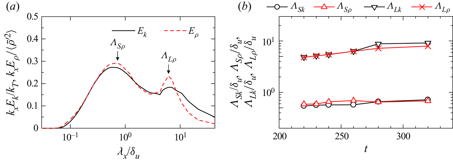
Figure 10. (a) Energy spectra of turbulent kinetic energy ( $E_k$) and density ( $E_\rho$) at $t=260$ with the definition of short and long peak-wavelengths. The spectra multiplied by $k_x$ are normalized by turbulent kinetic energy $k_T= (\langle {\bar {u}^\prime}{^2}\rangle +\langle {\bar {v}^\prime}{^2}\rangle +\langle {\bar {w}^\prime}{^2}\rangle )/2$ or density variance $\langle {\bar {\rho }^\prime}{^2}\rangle$. (b) Temporal evolution of short and long peak-wavelengths in $E_k$ and $E_\rho$. These results are taken at the centre of the shear layer in run 2.
The degree of anisotropy of the Reynolds stress tensor  $R_{ij}=\langle \bar {u}_{i}'\bar {u}_{j}'\rangle$ is evaluated with the normalized anisotropy tensor defined as
 \begin{equation} b_{ij}=\frac{R_{ij}}{R_{kk}}-\frac{1}{3}\delta_{ij}. \end{equation}
The state of anisotropy of  $R_{ij}$ is often expressed by the Lumley triangle, which is defined with $\eta _b=(b_{ij}b_{ji}/6)^{1/2}$ and $\xi _b=(b_{ij}b_{jk}b_{ki}/6)^{1/3}$ (Pope Reference Pope2000). The isotropic Reynolds stress has $(\xi _b,\eta _b)=(0,0)$. Although the Lumley triangle was also investigated in DNS of stratified shear layers (Smyth & Moum Reference Smyth and Moum2000a; Wingstedt et al. Reference Wingstedt, Fossum, Pettersson Reif and Werne2015), small computational domains used in previous DNS did not allow the growth of ELSS. However, the spectral energy density for ELSS is not negligible in figure 8, and the ELSS might have significant influences on the anisotropy of Reynolds stress. The Lumley triangle is often used for turbulence modelling but is used as a diagnostic tool for the isotropy of Reynolds stress in this study. Because $b_{ij}$ is defined with $R_{ij}$ normalized by $R_{kk}$, it is useful to compare $(\xi _b,\eta _b)$ among different flows even if these flows have different magnitudes of the turbulent kinetic energy. For example, Gargett & Wells (Reference Gargett and Wells2007) provided the discussion on $\eta _b$ and $\xi _b$ in observations of ocean turbulence by comparing them with canonical turbulent flows, such as turbulent boundary layers.
Figure 11(a) shows variations of  $(\xi _b,\eta _b)$ from $z=0$ to $0.5\delta _u$ at $t=140$ and $320$. The LES results (run 2) are compared with the results obtained at different heights of a turbulent boundary layer (Watanabe et al. Reference Watanabe, Zhang and Nagata2019b) and at the centre of a non-stratified, fully developed turbulent mixing layer (Takamure et al. Reference Takamure, Ito, Sakai, Iwano and Hayase2018). Here, the vertical location in the turbulent boundary layer, $y$, is normalized by the viscous length $\delta _\nu =\nu /u_\tau$ defined with the friction velocity $u_\tau =\sqrt {\tau /\rho }$ ( $\tau$: wall shear stress) as $y^{+}=y/\delta _\nu$. Three locations, $y^{+}=5$, $30$ and $800$, represent the approximate locations that separate the viscous sublayer ( $y^{+}\lesssim 5$), the buffer layer ( $5\lesssim y^{+}\lesssim 30$), the logarithmic layer ( $30\lesssim y^{+}\lesssim 800$) and the outer region ( $y^{+}\gtrsim 800$). At $t=140$, the centre of the stably stratified shear layer has $(\xi _b,\eta _b)\approx (0.08,0.1)$ (a green circle in figure 11a), which is close to the outer region of the turbulent boundary layer. At $t=320$, both $\xi _b$ and $\eta _b$ become large compared with early time. Here, the centre of the shear layer has $(\xi _b, \eta _b)=(0.16,0.17)$ (a red circle in figure 11a), and the Reynolds stress is more anisotropic than at the early time. In addition, $(\xi _b, \eta _b)\approx (0.16,0.17)$ is within the logarithmic layer in case of the turbulent boundary layer. On the other hand, the region away from the centreline still attains $(\xi _b, \eta _b)$ close to the outer region of the turbulent boundary layer.
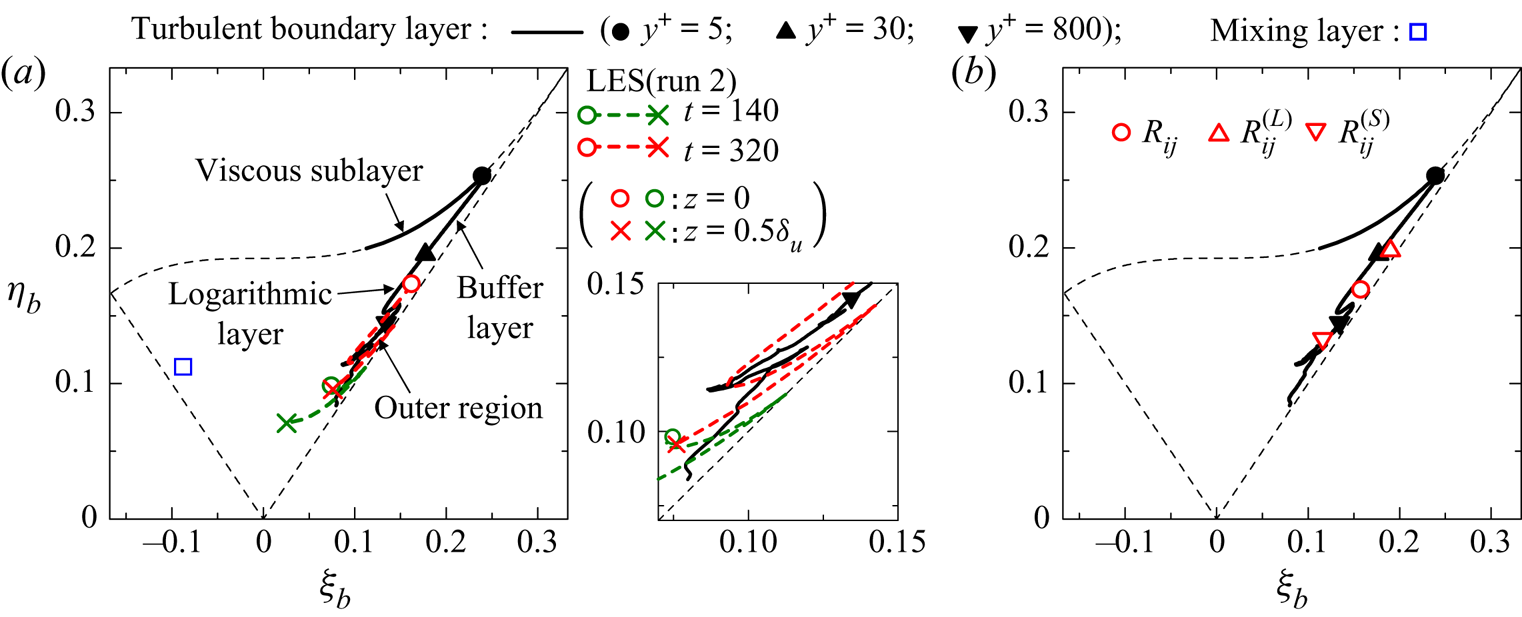
Figure 11. (a) Variation of  $\xi _b$ and $\eta _b$ between $z=0$ and $0.5\delta _u$ at $t=140$ and 320 in run 2. An enlarged figure is also shown for clarity. (b) Plots of $\xi _b$ and $\eta _b$ associated with large and small peak-wavelengths of the turbulent kinetic energy spectrum at $z=0$ and $t=320$ in run 2. Three thin broken lines correspond to an axisymmetric state with one large eigenvalue, $\eta _b=\xi _b$, or one small eigenvalue, $\eta _b=-\xi _b$, and a two-dimensional state $\eta _b=(1/27+2\xi _b^3)^{1/2}$. Figures also include $\xi _b$ and $\eta _b$ obtained in the turbulent boundary layer at the momentum thickness Reynolds number of ${Re}_{\theta }=13\,000$ in Watanabe et al. (Reference Watanabe, Zhang and Nagata2019b) and at the centre of the non-stratified, fully developed turbulent mixing layer (Takamure et al. Reference Takamure, Ito, Sakai, Iwano and Hayase2018).
The flow has two characteristic energy-containing length scales represented by  $\varLambda _{Sk}$ and $\varLambda _{Lk}$. We introduce $k_{min}$, which represents the wavenumber corresponding to the minimum value of $k_{x}E_k$ at $z=0$ between the two peaks at $\varLambda _{Sk}$ and $\varLambda _{Lk}$ (see figure 10a). The contributions to the Reynolds stress from fluctuations associated with $\varLambda _{Sk}$ (LSM) and $\varLambda _{Lk}$ (ELSS) are respectively evaluated by integrating a corresponding cospectrum as
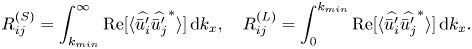 \begin{equation}
R_{ij}^{(S)}=\int_{k_{min}}^{\infty}{{\rm Re}}[\langle
\widehat{\bar{u}_{i}'}\widehat{\bar{u}_{j}'}^{*}\rangle]\,\textrm{d}k_x,\quad
R_{ij}^{(L)}=\int_{0}^{k_{min}}{{\rm Re}}[\langle
\widehat{\bar{u}_{i}'}\widehat{\bar{u}_{j}'}^{*}\rangle]\,\textrm{d}k_x.
\end{equation}
\begin{equation}
R_{ij}^{(S)}=\int_{k_{min}}^{\infty}{{\rm Re}}[\langle
\widehat{\bar{u}_{i}'}\widehat{\bar{u}_{j}'}^{*}\rangle]\,\textrm{d}k_x,\quad
R_{ij}^{(L)}=\int_{0}^{k_{min}}{{\rm Re}}[\langle
\widehat{\bar{u}_{i}'}\widehat{\bar{u}_{j}'}^{*}\rangle]\,\textrm{d}k_x.
\end{equation}
The anisotropy of velocity fluctuations associated with the LSM and ELSS is evaluated with  $\eta _b$ and $\xi _b$ calculated separately from $R_{ij}^{(S)}$ and $R_{ij}^{(L)}$. Figure 11(b) compares $\eta _b$ and $\xi _b$ obtained from $R_{ij}$, $R_{ij}^{(S)}$ and $R_{ij}^{(L)}$ at $z=0$ and $t=320$. For fluctuations associated with the large peak-wavelength, $(\eta _b,\xi _b)\approx (0.2,0.2)$ is obtained from $R_{ij}^{(L)}$. The turbulent boundary layer also has $(\eta _b,\xi _b)\approx (0.2,0.2)$ between the buffer layer and the logarithmic layer, and the anisotropy of the Reynolds stress for $\varLambda _{Lk}$ (ELSS) is similar to the near-wall region. However, $\eta _b$ and $\xi _b$ obtained from $R_{ij}^{(S)}$ are close to the values in the outer region. Therefore, the highly anisotropic Reynolds stress $R_{ij}$ near the centre of the shear layer is caused by the ELSS with an approximate length of $\varLambda _{Lk}$. In figure 11(a), $(\eta _b,\xi _b)$ near the edge of the shear layer at $t=320$ (a red cross in figure 11a) are still close to the values in the outer region of the turbulent boundary layer. This is explained by the absence of the ELSS near the edge of the stably stratified shear layer since the long-wavelength peak at $\lambda _x\approx \varLambda _{Lk}$ in the energy spectra does not exist at large $z$ in figure 8(c,f,i).
A fractional contribution to the total Reynolds stress from  $R_{ij}^{(L)}$ and $R_{ij}^{(S)}$ can be defined as $F_S = R_{ij}^{(S)}/R_{ij}$ and $F_L = R_{ij}^{(L)}/R_{ij}$ for each component of $i$ and $j$. Similarly, $F_S$ and $F_L$ for density variance $\langle {\bar {\rho }^\prime}{^2}\rangle$ and vertical density flux $\langle \bar {\rho }'\bar {w}'\rangle$ can be defined with the integral of the corresponding spectrum and cospectrum. Figure 12(a) shows temporal variations of $F_S$ and $F_L$ at $z=0$ for velocity and density variances. For all components, $F_S$ decreases and $F_L$ increases with time, and the contribution from the ELSS relatively becomes more important with time for velocity and density fluctuations. Figure 12(b) shows $F_S$ and $F_L$ obtained for the vertical turbulent fluxes of $u$ and $\rho$. Unlike velocity and density variances, $F_L$ stays around 0 even at late time, and the LSM with scales close to $\varLambda _{Sk}$ dominate the vertical transfer of momentum and density. The Reynolds stress and the vertical fluxes become small at late time, and $F_S$ and $F_L$ only provide the relative contribution at a given time. Therefore, large $F_L$ does not mean that the ELSS have a dominant contribution to the energetic property over the shear layer development. Figure 12(c) plots $R_{ij}^{(L)}$ and $R_{ij}^{(S)}$ for $(i,j)=(1,1)$ and $(1,3)$. Although $R_{11}^{(S)}$ decays with time, $R_{11}^{(L)} \approx 1$ slowly varies and the velocity fluctuations of the ELSS hardly decay. Similar results are obtained for $R_{22}$ and $R_{33}$ (not shown here). On the other hand, $R_{13}^{(L)}$ is close to 0 while $R_{13}^{(S)}$ also decreases to 0 with time. Thus, the ELSS hardly contribute to the vertical transport of momentum. Large scatters are found for $F_L$ and $F_S$ at late time in figure 12(b). This is caused by small $\langle \bar {u}'\bar {w}'\rangle$ and $\langle \bar {\rho }'\bar {w}'\rangle$, which are the denominators of $F_S$ and $F_L$. Figure 12(a,b) confirm that the ELSS carry an important fraction of the turbulent kinetic energy while the vertical transport of momentum due to the ELSS is not significant. This is due to the weak correlation between $u$ and $w$. In turbulent shear flows the decay of turbulent kinetic energy is caused by the viscous dissipation while the destruction of the Reynolds stress $\langle u'w'\rangle$ is caused by the pressure–strain correlation (Pope Reference Pope2000). The viscous dissipation is active at small scales. However, the destruction of the Reynolds stress actively occurs at larger scales than the viscous dissipation (Takahashi et al. Reference Takahashi, Iwano, Sakai and Ito2019). The different length scales of the decay process between the turbulent kinetic energy and the Reynolds stress is a possible reason for the weak vertical momentum transport by the ELSS with large turbulent kinetic energy.

Figure 12. Fractional contributions of fluctuations associated with long and short peak-wavelengths ( $F_L$ and $F_S$) of $E_k$ to (a) velocity and density variances, (b) vertical turbulent fluxes of streamwise velocity and density. (c) Reynolds stress associated with long and short peak-wavelengths, $R_{ij}^{(L)}$ and $R_{ij}^{(S)}$, for $(i,j)=(1,1)$ and $(1,3)$. Figure (d) shows $F_L$ and $F_S$ for the dissipation rates of turbulent kinetic energy and density variance. These results are taken at $z=0$ in run 2.
For the turbulent kinetic energy dissipation rate,  $F_S$ and $F_L$ are obtained by integrating $\hat {\varepsilon }^{(k)}= \hat {\varepsilon }_{G}^{(u)} +\hat {\varepsilon }_{G}^{(v)} +\hat {\varepsilon }_{G}^{(w)} +\hat {\varepsilon }_{S}^{(u)} +\hat {\varepsilon }_{S}^{(v)} +\hat {\varepsilon }_{S}^{(w)}$, i.e.
 \begin{equation} F_S=\frac{\displaystyle\int_{k_{min}}^{\infty} \hat{\varepsilon}^{(k)}\,\textrm{d}k_x} {\displaystyle\int_{0}^{\infty} \hat{\varepsilon}^{(k)} \,\textrm{d}k_x}, \quad F_L={=}\frac{\displaystyle\int_{0}^{k_{min}} \hat{\varepsilon}^{(k)} \,\textrm{d}k_x} {\displaystyle\int_{0}^{\infty} \hat{\varepsilon}^{(k)} \,\textrm{d}k_x}. \end{equation}
Similarly,  $F_S$ and $F_L$ for the dissipation rate of density variance are defined with the integrals of the dissipation term $\hat {\varepsilon }^{(\rho )} = \hat {\varepsilon }_{G}^{(\rho )} + \hat {\varepsilon }_{S}^{(\rho )}$. Figure 12 shows $F_S$ and $F_L$ for $\hat {\varepsilon }^{(k)}$ and $\hat {\varepsilon }^{(\rho )}$. Even at late time, $F_L$ is close to 0, and the ELSS have only a small contribution to the dissipation. It should be noted that $F_S\approx 1$ does not mean that the LSM causes the dissipation because $F_S$ includes the contribution from velocity and density fluctuations at smaller scales than the LSM.
3.5. Energy budget in wavenumber space
The spectral budget equations are analysed to investigate temporal evolutions of the spectra. Here, each term in the budget equations is premultiplied by  $k_x$, and is plotted as a function of $\lambda _x/\delta _u$ at a given location of $z/\delta _u$, where a logarithmic scale is used for $\lambda _x$. The LES results (run 2) are presented for $z/\delta _u=0$ and $0.4$ and for $t=140$ and 240 because the spectral shapes are very different between these heights and times. The diffusive terms $\hat {D}^{(u_\alpha )}$ and $\hat {D}^{(\rho )}$ in (2.14) and (2.16) are about $10^{1} - 10^{2}$ times smaller than other spatial transport terms, and these terms are not shown in this paper.
3.5.1. Spectral energy budget at early time
Figure 13(a–f) presents the spectral energy budget (2.14) at  $t=140$ for $E_u$, $E_v$ and $E_w$. The left and right columns of the figure show the results at $z=0$ and $0.4\delta _u$, respectively. In figure 13(a,b) the production term $\hat {P}^{(u)}$ is mostly positive for a wide range of $\lambda _x$. At both vertical locations, $\hat {P}^{(u)}$ peaks at $\lambda _x/\delta _u\approx 1$, and the energy production is the most active for the length scale close to $\delta _u$, i.e. the length scale of the LSM. This is consistent with canonical turbulent free shear flows, where the energy production occurs at large scales, which can be characterized by the width of the flow in the transverse (cross-flow) direction. Positive production can also be seen for very large scales $\lambda _x/\delta _u\approx 10^1$ at $z=0$, and the energy production at very large scales already occurs at the early time. This energy produced at $\lambda _x/\delta _u\approx 10^1$ is removed by the interscale transport term $\hat {T}_{S}^{(u)}$.
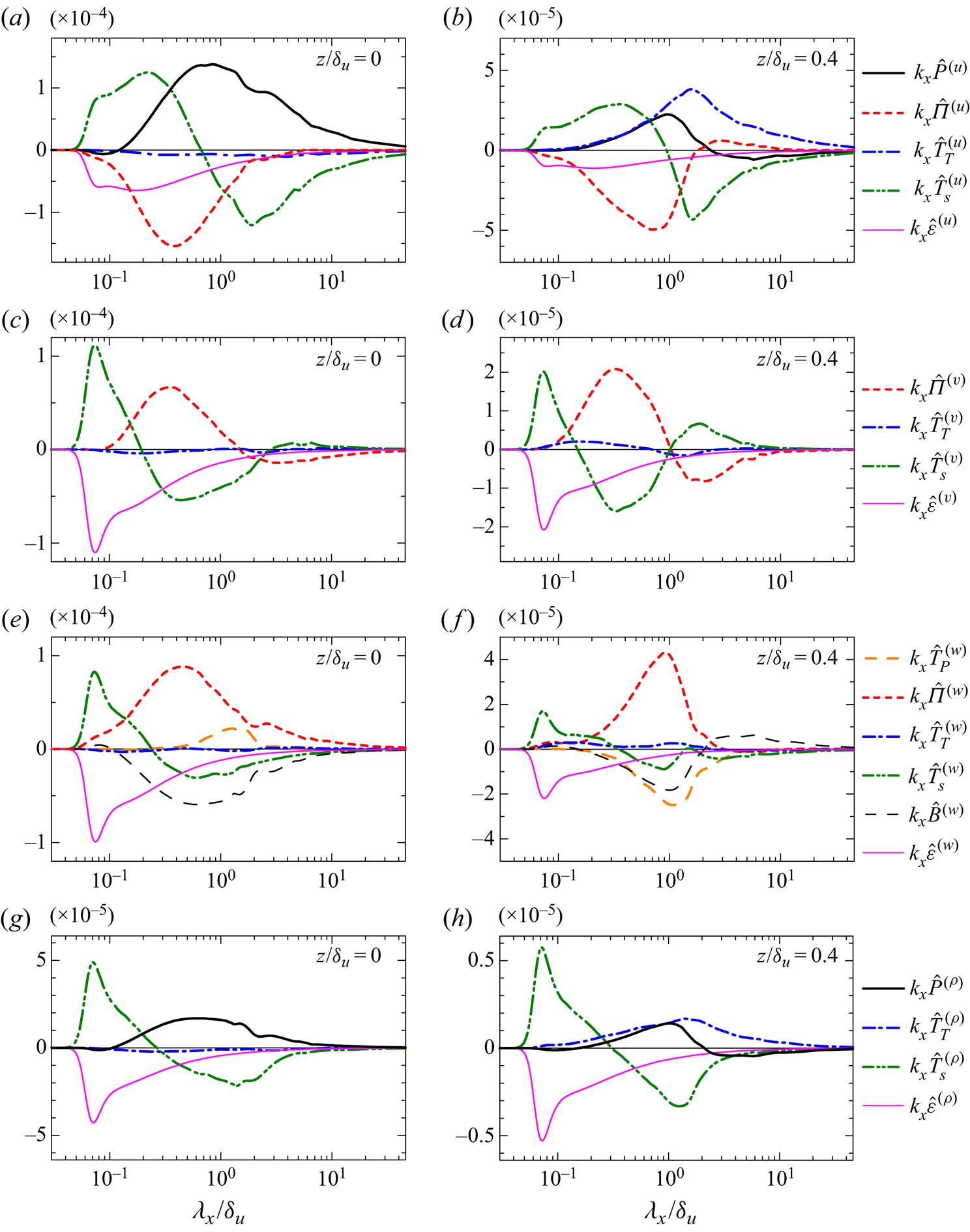
Figure 13. Spectral energy budgets of (a,b) streamwise velocity, (c,d) spanwise velocity, (e,f) vertical velocity and (g,h) density at  $t=140$ in run 2. Results are shown for (a,c,e,g) $z=0$ and (b,d,f,h) $z=0.4\delta _u$. Each term in the energy budget equations is plotted against the streamwise wavelength $\lambda _x=2{\rm \pi} /k_x$.
In figure 13(a,b) the pressure–strain correlation  $\hat {\varPi }^{(u)}$ is mostly negative, and large negative $\hat {\varPi }^{(u)}$ appears for the range of $\lambda _x$ with large positive $\hat {P}^{(u)}$. In figure 13(c–f), $\hat {\varPi }^{(v)}$ and $\hat {\varPi }^{(w)}$ tend to be positive for the wavelength with negative $\hat {\varPi }^{(u)}$. The energy of $\bar {u}'$, increased by the production, is partially redistributed to those of $\bar {v}'$ and $\bar {w}'$ at large scales close to $\lambda _x\approx \delta _u$. In figure 13(c), $\hat {\varPi }^{(v)}$ is negative for $\lambda _x/\delta _u\gtrsim 2$, for which $\hat {\varPi }^{(w)}$ in figure 13(e) is positive, and the energy is redistributed from $\bar {v}'$ mainly to $\bar {w}'$. The wavelength of this energy redistribution is larger than the peak wavelength of the positive energy production for $E_u$. Interestingly, similar behaviour of the pressure–strain correlation was reported in channel flows (Lee & Moser Reference Lee and Moser2019): the energy of the streamwise velocity is redistributed to the vertical (wall-normal) and spanwise velocity components at large scales, while for even larger scales, the energy of the spanwise velocity is redistributed to that of the vertical velocity.
The dissipation terms  $\varepsilon ^{(u_\alpha )}=\varepsilon _{G}^{(u_\alpha )}+\varepsilon _{S}^{(u_\alpha )}$ have a negative peak at small scales as expected from the scale dependence of the energy dissipation in turbulence. The turbulent diffusion terms $\hat {T}_{T}^{(u_\alpha )}$ are relatively small compared with other important terms at $z=0$ in figure 13(a,c,e). However, $\hat {T}_{T}^{(u)}$ at $z/\delta _u=0.4$ is the main source of the energy growth at large scales in figure 13(b). Pham & Sarkar (Reference Pham and Sarkar2010) also found that the turbulent kinetic energy is transferred outward in the stably stratified shear layer. On the other hand, $\hat {T}_{T}^{(v)}$ and $\hat {T}_{T}^{(w)}$ are smaller than other important terms even at $z/\delta _u=0.4$, where the pressure–strain correlation is the source of the energy.
The interscale transport term  $\hat {T}_{S}^{(u)}$ in figure 13(a,b) is positive for $\lambda _x/\delta _u \lesssim 0.8$ and is negative for larger scales. Similarly, positive and negative $\hat {T}_{S}^{(w)}$ in figure 13(e,f) can be found for small and large scales, respectively. Therefore, a forward energy transfer from large to small scales occurs for the energy of $\bar {u}'$ and $\bar {w}'$. However, $\hat {T}_{S}^{(v)}$ in figure 13(c,d) exhibits negative values for $0.2\lesssim \lambda _x/\delta _u \lesssim 2$, which are surrounded by positive values for larger and smaller scales. This profile indicates that the energy at scales of $0.2\lesssim \lambda _x/\delta _u \lesssim 2$ is transferred to both large and small scales. Positive $\hat {T}_{S}^{(v)}$ for $\lambda _x/\delta _u \gtrsim 2$ appears for the wavelength with negative $\hat {\varPi }^{(v)}$. Therefore, the interscale energy transfer of $\bar {v}'$ feeds the energy at large scales, which is further redistributed by the pressure–strain correlation. At $t=140$, the Ozmidov scale is $L_O/\delta _u=6.9\times 10^{-2}$ at the centre of the shear layer. Turbulent motions with scales greater than the Ozmidov scale are expected to be strongly suppressed by the buoyancy (Riley & Lindborg Reference Riley and Lindborg2008). However, $\hat {T}_{S}^{(u_\alpha )}$ confirms that the forward energy transfer occurs for length scales larger than the Ozmidov scale, indicating that the active interscale transport in the turbulent shear layer is possible even under the strong influence of stable stratification. It is interesting to note that the scale dependence of $\hat {T}_{S}^{(u_\alpha )}$ in the stably stratified shear layer is consistent with DNS results of channel flows (Lee & Moser Reference Lee and Moser2019). Above the buffer layer of the channel flow, an interscale transfer from large to small scales occurs for the energy of streamwise and vertical velocities while the energy of spanwise velocity is transferred to both large and small scales.
The pressure diffusion and buoyancy flux terms appear only in the equation for  $E_w$ shown in figure 13(e,f). The pressure diffusion term for $\lambda _x/\delta _u\approx 10^0$ is positive at $z=0$ and negative at $z/\delta _u=0.4$, and transfers the energy toward the middle of the shear layer at large scales. The profile of the buoyancy flux is similar to the pressure–strain correlation with opposite signs, and the energy converted to $w'$ is partially removed by the buoyancy force.
Figure 13(g,h) shows the spectral energy budget of density fluctuations, (2.16), at  $t=140$. Both streamwise velocity and density fluctuations are produced by the vertical gradients of $\langle u \rangle$ and $\langle \rho \rangle$, whose initial profiles are given by a hyperbolic tangent function. Therefore, the spectral energy budget is similar between $E_u$ and $E_\rho$ at $t=140$.
3.5.2. Spectral energy budget at late time
Figure 14(a–f) presents the spectral energy budget at  $t=240$ for three velocity components. At $t=240$, $E_u$ and $E_\rho$ have a second peak associated with the ELSS while the long-wavelength peak is forming in $E_v$ and $E_w$ (figure 8). For $E_{u}$, the dissipation, turbulent transport and interscale transfer terms are qualitatively similar at $t=140$ and 240 while $\hat {P}^{(u)}$ and $\hat {\varPi }^{(u)}$ have different profiles. The production $\hat {P}^{(u)}$ at $t=240$ has a large peak at $\lambda _x/\delta _u\approx 0.6$ at both heights. At $z=0$, $\hat {P}^{(u)}$ has a second peak for $\lambda _x/\delta _u\approx 10$, which does not exist at $t=140$. The energy production for $\lambda _x/\delta _u\approx 10$ does not occur at $z/\delta _u=0.4$, where the ELSS do not appear. Negative $\hat {\varPi }^{(u)}$ appears for $0.1\lesssim \lambda _x/\delta _u \lesssim 1$, where the production term has large positive values. As also found at early time, the energy produced by the mean velocity gradient is redistributed to other velocity components for this wavelength range. However, this energy redistribution does not occur at $\lambda _x/\delta _u\approx 10$, where the energy production is active. Comparisons of all terms shown in figure 14(a) imply that the growth of the ELSS at $\lambda _x/\delta _x\approx 10^1$ is mainly caused by the energy production at very large scales.
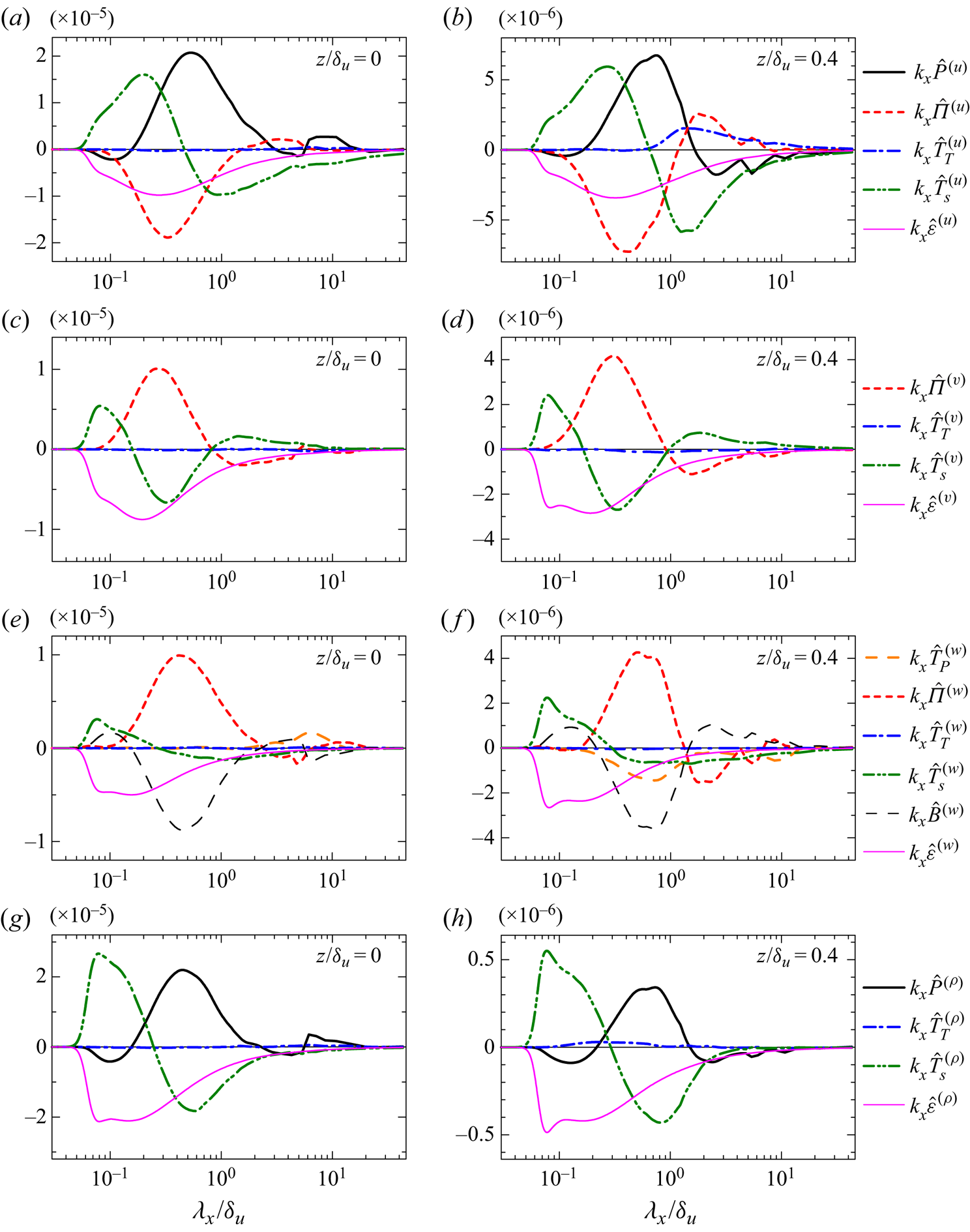
Figure 14. Same as figure 13, but at  $t=240$.
The most terms for the budget of  $E_v$ are qualitatively similar between $t=140$ and 240. However, negative $\hat {\varPi }^{(v)}$ at $\lambda _x/\delta _u \gtrsim 5$ found at $t=140$ is not observed at $t=240$, and $\hat {\varPi }^{(v)}$ does not cause the decay of $E_v$ at very large scales. For $E_{w}$, time dependence is significant for $\hat {T}_{P}^{(w)}$ and $\hat {\varPi }^{(w)}$. The pressure diffusion $\hat {T}_{P}^{(w)}$ at $t=240$ is positive at $\lambda _x/\delta _u\approx 10$ while $\hat {\varPi }^{(w)}$ is close to 0 for $\lambda _x/\delta _u\gtrsim 2$ at $t=240$. Thus, the pressure effect contributes to the energy growth at very large scales at $z=0$.
Figure 14(g,h) shows the budget of  $E_{\rho }$ at $t=240$. Difference between $t=140$ and 240 is similar for $E_u$ and $E_\rho$. A long-wavelength peak of the production term appears at $\lambda _x/\delta _u\approx 10$ at $t=240$ in figure 14(g), and the production at the very large scales generates the density fluctuations of ELSS.
One of the noteworthy features for the budgets of  $E_{u}$ and $E_{\rho }$ is small negative production at small scales of $\lambda _{x}/\delta _{u}\approx 0.1$ in figure 14(a,b,g,h). Even at $t=140$, the production terms have small negative values for $\lambda _x/\delta _u\approx 0.1$ in figure 13(a). These negative values of the production terms are also found in DNS (not shown here) and are not artificially caused by the implicit SGS model. The negative production requires ${{Re}}[\langle \widehat {\bar {u}'}^{*}\widehat {\bar {w}'}\rangle ] > 0$ and ${{Re}}[\langle \hat {\bar {\rho }'}^{*}\widehat {\bar {w}'}\rangle ]<0$. These cospectra represent the spectral density of the turbulent fluxes. The signs of the cospectra corresponding to the negative production are associated with the counter-gradient transports of streamwise momentum and density. This is contrary to the spectral analysis of Reynolds stress of a fully developed turbulent mixing layer without density stratification, where the turbulent momentum transport is in the down-gradient direction for all length scales (Takamure et al. Reference Takamure, Ito, Sakai, Iwano and Hayase2018). Interestingly, negative values of the production term of the turbulent kinetic energy spectrum were also found in channel flows (Lee & Moser Reference Lee and Moser2019). Around vertical locations between the buffer layer and logarithmic layer of the channel flow, the production term has large positive values at large scales while negative production appears for slightly smaller wavelengths than the positive production. As in the stably stratified shear layer considered in this study, the negative production in the channel flow is small compared with their positive peak at large scales.
3.5.3. Formation of double-peak energy spectra on the shear layer centreline
From  $t=140$ to $240$, the spectral shape at $z=0$ changes from a single-peak profile to a double-peak profile. The formation of the double-peak spectrum can be clearly appreciated by $T_\alpha ^{-1} \equiv (\partial E_{\alpha }/\partial t)/E_{\alpha }$, which can be interpreted as the rate (inverse of time scale) of the spectral evolution. Figure 15 shows $T_\alpha ^{-1}$ for three velocity components and density at $t=140$ and 240 at the centre of the shear layer. For $\lambda _x/\delta _u\lesssim 0.1$, $T_\alpha ^{-1}$ becomes large as $\lambda _x$ decreases. This is because the energy spectra become extremely small as the implicit SGS model dissipates the energy at resolved small scales. The energy spectra decay with time as also confirmed from $T_\alpha ^{-1}<0$ for most wavelengths. At $t=240$, the decay rate is small at $\lambda _x/\delta _u\approx 10$, which is the length scale of the ELSS. Therefore, the velocity fluctuations of the ELSS decay more slowly than those of the LSM. The scale dependence of $T_\alpha ^{-1}$ suggests that the spectrum with a single peak rapidly decays with time except for very large scales, and eventually the double-peak spectrum is formed once the spectrum decays sufficiently except for $\lambda _x/\delta _u\approx 10$. At $t=140$ in figure 15(a), the slow decay of energy spectra at $\lambda _x/\delta _u\approx 10$ is found only for $E_u$ and $E_\rho$. Thus, the decay of $E_v$ and $E_w$ is faster at larger scales. Consistently, the formation of the double-peak spectra occurs at earlier time for $E_u$ and $E_\rho$ than for $E_v$ and $E_w$ in figure 8.
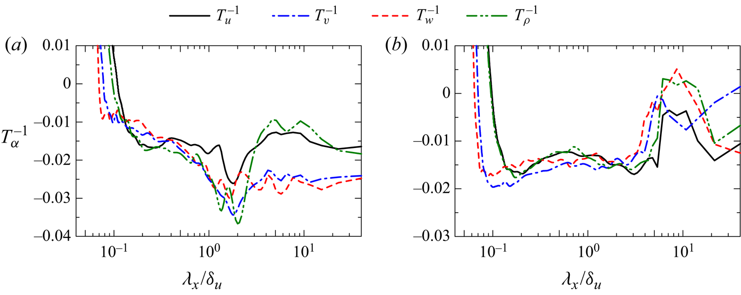
Figure 15. The rate of the change in energy spectra defined as  $T_{\alpha }^{-1}=(\partial E_{\alpha }/\partial t)/E_{\alpha }$ for $\alpha =u, v, w$ and $\rho$ at $z=0$ in run 2: (a) $t=140$; (b) $t=240$.
Figure 16(a) shows the production term  $k_{x}\hat {P}^{(u)}$ normalized by its maximum value $[k_{x}\hat {P}^{(u)}]_{max}$ at $z=0$ at four time instances. At $t=140$, the energy is produced for a wide range of length scales. However, the shape of $k_{x}\hat {P}^{(u)}$ changes from $t=140$ to 230, and the production term at late time has two peaks corresponding to the peaks in $E_u$. The energy production at $\lambda _x/\delta _u\approx 10$ becomes more important at late time. The production is almost zero or can be negative for $\lambda _x/\delta _u\approx 6$. This negligible production is consistent with $E_u$ in figure 8(c), where $E_u$ is locally small for the wavelength with small $k_{x}\hat {P}^{(u)}$. The wavelength of positive production corresponding to the long-wavelength peak is shifted to larger scales with time as also expected from the increase of the long peak-wavelength in figure 10(b). Figure 16(b) shows the sum of the pressure terms, $\hat {P}_{r}^{(w)}=\hat {T}_{P}^{(w)}+\hat {\varPi }^{(w)}$, at $z=0$, where $\hat {P}_{r}^{(w)}$ is premultiplied by $k_x$ and normalized by the maximum value of $k_x\hat {P}_{r}^{(w)}$. The pressure terms of $E_w$ play a similar role to the production term of $E_u$: the energy growth at $\lambda _x/\delta _u\approx 0.5$ and 10 is caused by the pressure effects for $E_{w}$ and by the production for $E_{u}$. The pressure effects are responsible for the change in the shape of $E_w$. Similar time dependence was found for the production term of density (not shown here). For $E_v$, we cannot identify a single term that is responsible for the formation of the double-peak spectrum. The growth of $E_v$ at large $\lambda _x$ is dominated by the interscale energy transfer $\hat {T}_{S}^{(v)}$ in figure 14(c), where the energy transfer from small to large scales occurs. The decrease of $E_v$ by the pressure–strain correlation for $\lambda _x/\delta _u\approx 10$ occurs at $t=140$ but not at $t=240$ as shown in figures 13(c) and 14(c). The balance of these terms causes the slow decay rate of very large-scale fluctuations in figure 15(b).
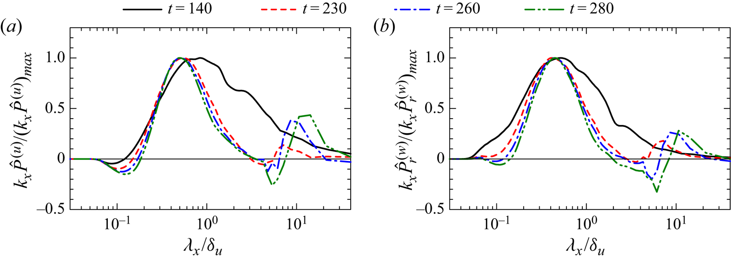
Figure 16. Temporal variations of (a) production term  $\hat {P}^{(u)}$ of $E_u$ and (b) pressure term $\hat {P}_{r}^{(w)}=\hat {\varPi }^{(w)}+\hat {T}_{P}^{(w)}$ of $E_w$ on the centreline ( $z=0$) in run 2. The terms $k_{x}\hat {P}^{(u)}$ and $k_{x}\hat {P}_{r}^{(w)}$ are normalized by their maximum values, $[k_{x}\hat {P}^{(u)}]_{max}$ and $[k_{x}\hat {P}_{r}^{(w)}]_{max}$.
3.6. Scaling of energy spectrum and structure function
Another interesting feature in the energy spectra in figure 8 is that the premultiplied spectrum at a fixed height is roughly constant for a certain wavenumber range at  $t=320$, implying a $k_x^{-1}$ power law. For example, $k_xE_{u}$ in figure 8(c) weakly depends on the wavenumber for $2\lesssim \lambda _x/\delta _u\lesssim 4$ near the centreline, while the range with constant $k_xE_{u}$ extends to smaller scales at $z/\delta _u\approx 0.25$, where large peaks at $\lambda _x/\delta _u\approx 1$ and 10 do not exist. As discussed above, some terms of the spectral energy equations have similar wavenumber dependence in the stably stratified shear layer and wall-bounded shear flows. Furthermore, turbulent structures that have been observed in the wall-bounded shear flows were also observed in the stably stratified shear layer, e.g. hairpin vortices and ELSS (Watanabe et al. Reference Watanabe, Riley, Nagata, Matsuda and Onishi2019a). Both stable stratification and a wall cause the suppression of vertical turbulent motions, which may lead similar turbulent characteristics in these flows. Interestingly, the scaling $E_{u}\sim k_x^{-1}$ has also been predicted and experimentally confirmed in wall turbulence (Perry & Chong Reference Perry and Chong1982; Nickels et al. Reference Nickels, Marusic, Hafez and Chong2005). The equivalent scaling in real space can be written with the velocity structure function, which is defined as $\langle (\Delta u)^2\rangle =\langle [\bar {u}(x+r,y,z)-\bar {u}(x,y,z)]^2\rangle$ with a separation distance $r$ in the $x$ direction. The scaling law of $\langle (\Delta u)^2\rangle$ corresponding to $E_{u}\sim k_{x}^{-1}$ is the logarithmic law given by $\langle (\Delta u)^2\rangle \sim \ln (r)$ (Davidson, Nickels & Krogstad Reference Davidson, Nickels and Krogstad2006). The physical basis underlying these scaling laws is the existence of turbulent motions with a range of scales which are characterized by a common velocity scale. Davidson et al. (Reference Davidson, Nickels and Krogstad2006) also pointed out that the logarithmic law is more easily observed than the $k_x^{-1}$ law because of the aliasing problem of one-dimensional spectra.
Figure 17(a–c) shows the structure functions of  $u$,
$u$,  $v$ and $w$ at $t=320$ at three vertical locations. Here, the structure functions of $v$ and $w$ are $\langle (\Delta v)^2\rangle =\langle [\bar {v}(x+r,y,z)-\bar {v}(x,y,z)]^2\rangle$ and $\langle (\Delta w)^2\rangle =\langle [\bar {w}(x+r,y,z)-\bar {w}(x,y,z)]^2\rangle$. Except near the edge of the shear layer ( $z/\delta _u=0.46$), the logarithmic law is valid for a certain range of large scales. The broken lines in (a) represent $\langle (\Delta u)^2\rangle = A + B\ln (r)$ with $A$ and $B$ obtained by the least square method, which is applied for $1.2 \leqslant r/\delta _u \leqslant 2.8$ at $z=0$ and $0.4\leqslant r/\delta _u \leqslant 2.8$ at $z/\delta _u=0.23$. In figure 17(b,c) the logarithmic law is also shown with the broken lines, which are obtained with the least square method applied for $0.97 \leqslant r/\delta _u \leqslant 2.4$ at $z=0$ and $0.81 \leqslant r/\delta _u \leqslant 1.6$ at $z/\delta _u=0.23$. The logarithmic law holds for all velocity components. However, $A$ and $B$ are not universal and are different for each velocity component and vertical location. Figure 17(d) shows the premultiplied spectrum $k_{x}E_{u}$ at the same locations. Although there is a range of $k_x$ where $k_{x}E_{u}$ weakly depends on $k_x$, this wavenumber range of constant $k_{x}E_{u}$ at $z=0$ is not as clear as the $\ln (r)$ law in figure 17(a), as also expected from the comparison between the $k_{x}^{-1}$ and logarithmic laws in turbulent boundary layers (Davidson et al. Reference Davidson, Nickels and Krogstad2006). Near the centre of the shear layer, $E_{\alpha }\sim k_{x}^{-1}$ tends to appear for the scales between two peaks in figure 8(c,f,i). In figure 8(c), $E_u$ does not have large peaks at $z/\delta _u\approx 0.25$, where the logarithmic law is valid for a wide range of scales in figure 17(a). Therefore, the logarithmic law is clearly observed for large scales when the scales are not affected by the spectral peaks of LSM and ELSS. As the scale separation between LSM and ELSS increases with time, the $\ln (r)$ law and $k^{-1}$ law may be more clearly observed at further later time.
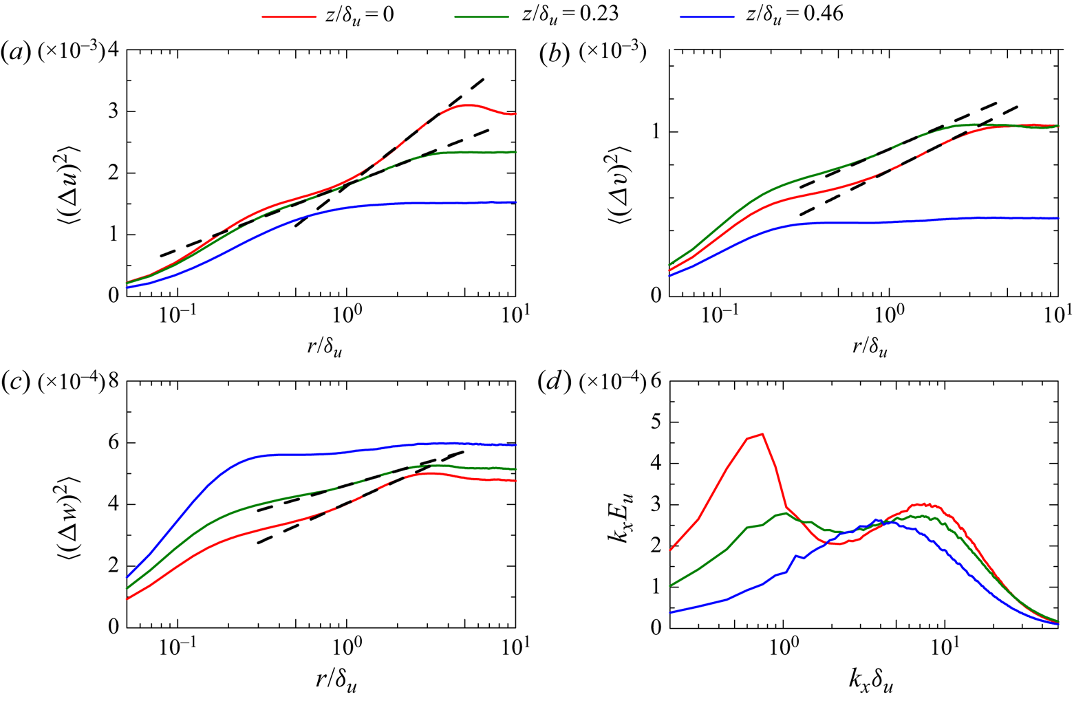
Figure 17. Structure functions of (a) streamwise velocity  $\langle (\Delta u)^2\rangle$, (b) spanwise velocity $\langle (\Delta v)^2\rangle$ and (c) vertical velocity $\langle (\Delta w)^2\rangle$ at $t=320$. The broken lines represent $A \ln (r/\delta _u)+B$ with $A$ and $B$ obtained with the least square method applied for $z=0$ and $0.23\delta _u$. (d) Premultiplied energy spectrum of streamwise velocity, $k_xE_u$, at $t=320$. These results are taken at $z/\delta _u=0$, $0.23$ and $0.46$ in run 2.
3.7. Comparison between the stably stratified shear layer and wall turbulence
The ELSS develop at late time in the stably stratified shear layer. Similar structures, known as superstructures or very LSM, also exist in wall-bounded turbulent shear flows, e.g. channel, pipe and boundary-layer flows (Hutchins & Marusic Reference Hutchins and Marusic2007; Monty et al. Reference Monty, Hutchins, Ng, Marusic and Chong2009). It was also shown that a large number of hairpin vortices exist in the stably stratified shear layer, where the hairpin vortices induce velocity fluctuations at the streamwise length scale of LSM (Watanabe et al. Reference Watanabe, Riley, Nagata, Matsuda and Onishi2019a). Thus, the stably stratified shear layer at late time resembles the wall turbulence in terms of the turbulent structures. Furthermore, the LES results presented above also confirm that some statistics are also qualitatively similar in these flows, e.g. the energy budget in wavenumber space, the anisotropy of Reynolds stress tensor and the logarithmic law of the velocity structure functions at large scales.
As confirmed from the energy spectra, the ELSS emerge at late time for  ${Re}=2000$ and 40 000 when $Ri$ is not too small. The detailed process of turbulent transition depends on the Reynolds number and Richardson number (Mashayek & Peltier Reference Mashayek and Peltier2012; Thorpe Reference Thorpe2012). Therefore, the transition process is not directly related to the formation of ELSS. This is also supported by the flow visualization in figure 4: the velocity fluctuations of the ELSS are hardly correlated with the velocity profiles associated with the Kelvin–Helmholtz instability and the initial velocity fluctuations. The spectral energy budget in § 3.5 also confirms that the flow dynamics is similar between the stably stratified shear layer and channel flow. Therefore, it is reasonable to assume that the ELSS in these flows are generated by the same mechanism. However, there is also a possibility that the ELSS is generated and sustained by long internal gravity waves, which may dominate the velocity fluctuations at the late time. Further investigation is required to clarify the generation mechanism of the ELSS. The ELSS develop even if ${Re}_b$ is larger than 100 ( ${Re}=40\,000$, $Ri=0.06$). The present LES suggests that $Ri$ or $Ri_g$ is an important parameter in the development of the ELSS because the ELSS are not observed for $({Re},Ri)=(40\,000,0.02)$, for which $Ri_g$ in table 2 is below the critical Richardson number 1/4 (Miles Reference Miles1961). On the other hand, the ELSS are observed for $Ri=0.06$ and 0.1, for which $Ri_g$ exceeds the critical value. At $Ri=0$ and 0.02, $\delta _u$ grows with time even at late time in figure 7(a). However, $\delta _u$ hardly increases with time for $Ri=0.06$ and 0.1 after the turbulent transition, and the vertical length scale of the flow does not vary with time. In wall turbulence the largest vertical length scale of turbulence at a given height is also fixed as the distance from the wall. The confinement of the growth of the vertical length scale is possibly important in the formation of the ELSS in these flows.
Negative production of  $E_u$ and $E_\rho$ at small scales is observed in figure 14(a,b,g,h). As explained above, the negative production is due to the counter-gradient transport of streamwise momentum and density. Previous studies on stratified turbulence also observed the counter-gradient transport regardless of the presence of mean shear (Lienhard & van Atta Reference Lienhard and van Atta1990; Holt, Koseff & Ferziger Reference Holt, Koseff and Ferziger1992; Komori & Nagata Reference Komori and Nagata1996). However, the physical mechanism of the counter-gradient transport in stratified turbulence may depend on the mean shear as discussed in Gerz & Schumann (Reference Gerz and Schumann1996). They explained the counter-gradient transport at small scales in stratified turbulence with mean shear based on the collision of fluid parcels which are vertically transferred by inclined hairpin vortices generated by the mean shear. Indeed, a large number of hairpin vortices develop in the stably stratified shear layer (Watanabe et al. Reference Watanabe, Riley, Nagata, Matsuda and Onishi2019a). Gerz & Schumann (Reference Gerz and Schumann1996) also suggested that the same mechanism can also cause the counter-gradient transport of momentum in wall-bounded shear flows, where the hairpin vortices have also been found in numerous studies (e.g. Wu & Moin Reference Wu and Moin2009). The wavenumber dependence of the production terms of $E_u$ and $E_\rho$ is also qualitatively similar between the middle of the shear layer (figure 14a) and the buffer and logarithmic layers of channel flows (Lee & Moser Reference Lee and Moser2019). Thus, the mechanism of the counter-gradient momentum transport proposed by Gerz & Schumann (Reference Gerz and Schumann1996) seems to be valid in these flows.
The integral shear parameter  $S^{*}=Sq^2/\varepsilon ^{(k)}$ ( $q^2=\langle u'_i u'_i\rangle$) represents the time scale ratio of the eddy turnover time $q^2/\varepsilon ^{(k)}$ to the mean-shear time scale $S^{-1}=\langle \partial u / \partial z \rangle ^{-1}$. The evolution of turbulence is strongly influenced by the mean shear when $S^{*}$ is much larger than $1$. Non-stratified turbulent free shear flows have $S^{*}\approx 3$– $6$ (Pope Reference Pope2000) while the stably stratified turbulent shear layer at $z=0$ has $S^{*}\geqslant 10$, which continuously increases with time. At $({Re},Ri)=(2000,0.06)$, $S^{*}$ reaches about 30 at $t=320$ (Watanabe et al. Reference Watanabe, Riley, Nagata, Matsuda and Onishi2019a) and $S^{*}\approx 30$ is as large as in the buffer layer of channel flows (Jiménez Reference Jiménez2013). The counter-gradient transport by the mechanism proposed in Gerz & Schumann (Reference Gerz and Schumann1996) is simply due to the strong influence of mean shear and is not directly related to the stable stratification. Therefore, the counter-gradient momentum transport at small scales occurs in homogeneous shear flow with $S^{*}\approx 30$ even without stable stratification (Iida & Nagano Reference Iida and Nagano2007), where the shape of the cospectrum of the vertical momentum-flux is qualitatively similar to $\hat {P}^{(u)}$ in figure 16(a) except the scales of the ELSS. The mean shear $S$ in a temporally evolving, turbulent shear layer decreases with time in the absence of stable stratification because the shear layer thickness increases. Therefore, although the eddy turnover time $q^2/\varepsilon ^{(k)}$ becomes large with time, $S^{*}$ stays small and the counter-gradient transport does not occur without stable stratification (Takamure et al. Reference Takamure, Ito, Sakai, Iwano and Hayase2018). The stable stratification suppresses the growth of the shear layer thickness. Thus, $S\sim U_0/\delta _u$ hardly varies with time while $S^{*}$ increases with time because of the increase of the eddy turnover time. Therefore, the stably stratified shear layer at late time has large $S^{*}$, and the strong influence of the mean shear can result in the counter-gradient transport at small scales.
4. Conclusions
Direct numerical simulation and implicit LES were performed for a temporally evolving, stably stratified turbulent shear layer with a large computational domain that can contain ELSS. The moderate computational cost of LES enabled us to repeat the simulations with different initial velocity fluctuations and to perform ensemble averages, which are difficult in DNS because of the computational cost. The statistics calculated with ensemble averages allowed detailed quantitative investigations of statistics related to large-scale flow characteristics. The main analyses were reported for  ${Re}=2000$ and $Ri=0.06$, for which the Kelvin–Helmholtz instability generates turbulence. As summarized below, some statistics reported in this paper qualitatively agree with those in channel and boundary-layer flows, indicating similar flow dynamics in the stratified shear layer and wall-bounded shear flows.
The shape of the energy spectra calculated with Fourier transform in the streamwise direction drastically changes with time: the velocity and density spectra near the centreline have a single peak in the wavenumber space at early time and double peaks at late time. Thus, the flow at late time has two energy-containing length scales. One is close to the shear layer thickness, which is a typical scale of LSM of turbulent mixing layers even without stable stratification. This energy-containing length scale exists even at early time. The other length scale is larger than the shear layer thickness and is close to the streamwise length of ELSS, which are visualized as positive and negative velocity fluctuations on horizontal planes. Large eddy simulations with  ${Re}=40\,000$ confirmed that the ELSS appear at $Ri=0.06$ and 0.1 but not at $Ri=0$ and 0.02. The streamwise length scale of LSM hardly changes with time while that of ELSS monotonically increases. The length of the ELSS reaches about 10 times the shear layer thickness. The LSM exists in the entire shear layer while the ELSS appears only near the centreline at late time. The velocity and density fluctuations of the ELSS hardly decay with time. Therefore, the contributions of the ELSS to velocity and density variances become important with time and account for about 50 % of velocity and density fluctuations at late time. However, the vertical turbulent transport of momentum and density are still dominated by the LSM. The ELSS also hardly contributes to the dissipation of velocity and density fluctuations. The Reynolds stress associated with the ELSS is highly anisotropic, with a degree of anisotropy on a Lumley triangle close to the near-wall region of a turbulent boundary layer. However, the LSM has Reynolds stress which is as anisotropic as in the outer region of the turbulent boundary layer.
The budget equations were evaluated for the velocity and density spectra ( $E_{u}$, $E_{v}$, $E_{w}$ and $E_\rho$). The interscale energy flux transfers the energy of streamwise velocity fluctuations $u'$ and vertical velocity fluctuations $w'$ from large to small scales while the energy of spanwise velocity fluctuations $v'$ is transferred to both large and small scales. Before the ELSS has developed, the energy of $v'$ at very large scales is converted mainly to the energy of $w'$ by the pressure–strain correlation, where the source of this energy conversion is the interscale energy transfer of $v'$ from small scales. The production terms of $E_u$ and $E_\rho$ have a peak at the scales of LSM while they become negative at slightly smaller scales than the scales with the positive production. These negative productions are related to the counter-gradient transport of streamwise momentum and density. The spectral analysis of channel flows also found similar behaviour of the production, pressure–strain correlation and interscale energy transfer terms (Lee & Moser Reference Lee and Moser2019). Once the ELSS has developed, the production terms of $E_u$ and $E_\rho$ have two peaks near the centre of the shear layer, where the energy is produced at the wavelengths of the LSM and ELSS. Furthermore, the role of the pressure terms of $E_w$ is similar to the production of $E_u$: the growth of $E_w$ by the pressure terms occurs at the wavelengths of the LSM and ELSS. When the double-peak spectra are forming at late time, the decay of the energy spectrum at the scales of ELSS is much slower than at the small scales of LSM. This slow decay rate of the large-scale fluctuations results in the formation of the ELSS.
The scaling of the energy spectrum at large scales was also explored in comparison with wall-bounded turbulent shear flows. The present LES suggested that the logarithmic law of the velocity structure functions holds for large scales in the stably stratified shear layer. The logarithmic law for the structure function of  $u$ was observed for a wide range of the scales at vertical heights where the energy spectrum does not have large peaks of the LSM and ELSS. The corresponding scaling of the energy spectrum is the $k_x^{-1}$ law although the clear $k_x^{-1}$ law seems to be more difficult to observe as suggested by previous studies on turbulent boundary layers (Davidson et al. Reference Davidson, Nickels and Krogstad2006).
Direct numerical simulations of a stably stratified shear layer have been widely used to assess various parameters related to turbulent mixing in the existing literature. However, most previous studies used small computational domains, where the ELSS could not grow because of confinement effects. Thus, the existence of ELSS can alter findings in previous DNS if the ELSS play important roles in the flow evolution. It was shown that the ELSS holds a large fraction of turbulent kinetic energy. This might be important from a viewpoint of turbulence modelling because the ELSS with large velocity fluctuations may affect the dissipation scaling  $\varepsilon \sim {\mathcal {U}}^{3}/{\mathcal {L}}$ that relates the kinetic energy dissipation rate $\varepsilon$ to the characteristic velocity and length scales, ${\mathcal {U}}$ and ${\mathcal {L}}$, of large-scale (horizontal) turbulent motions. This relation is often used in theoretical studies on stratified turbulence (Riley & Lindborg Reference Riley and Lindborg2008; Caulfield Reference Caulfield2021). A detailed investigation of the assumptions made in turbulence modelling should also be conducted in future studies.
Acknowledgements
The numerical simulations presented in this paper were carried out on the high-performance computing system (NEC SX-ACE) in the Japan Agency for Marine-Earth Science and Technology.
Funding
This work was partially supported by ‘Collaborative Research Project on Computer Science with High-Performance Computing in Nagoya University’ and by JSPS KAKENHI, grant numbers 18H01367 and 20H05754.
Declaration of interests
The authors report no conflict of interest.
Appendix A. Effects of the computational domain size on the stably stratified shear layer
The periodic boundary condition in the horizontal direction may affect the development of a stably stratified shear layer when the computational domain is not sufficiently large. Previous studies often used a much smaller domain than present DNS and LES. In this appendix it will be shown that the small domain has non-negligible influences on both transitional and fully developed turbulent regimes of the stably stratified shear layer. We have conducted an additional DNS, run 7, for  $({Re},Ri,Pr)=(2000, 0.06, 1)$ with a small computational domain as summarized in table 3. The domain size in the horizontal direction is comparable to those used in previous studies (Smyth & Moum Reference Smyth and Moum2000a; Mashayek & Peltier Reference Mashayek and Peltier2013; Kaminski & Smyth Reference Kaminski and Smyth2019; VanDine, Pham & Sarkar Reference VanDine, Pham and Sarkar2021). The grid stretching parameter is $\alpha _z=4$ in run 7 and the spatial resolution in the shear layer is comparable in runs 1 and 7. The initial velocity perturbation is also generated by the same method for these runs. Direct numerical simulations of run 7 are repeated for $N_S=16$ times, which are used to take ensemble averages.
Table 3. Computational parameters of DNS used for the assessment of the domain size effects.
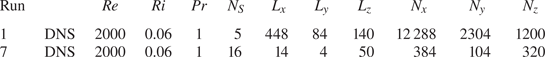
Figure 18 visualizes density  $\rho$ at $t=60$ in run 7. The streamwise length $L_x=14$ is about twice the streamwise wavelength of the most unstable Kelvin–Helmholtz instability mode. Therefore, two roller vortices of the Kelvin–Helmholtz instability are observed in figure 18(a). The horizontal profile of $\rho$ at $z=0$ in figure 18(b) is almost uniform in the $y$ direction and the quasi-two-dimensional vortices are developing at $t=60$.
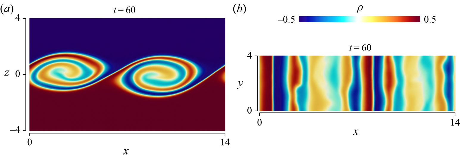
Figure 18. Density profiles on (a) an  $x$–
$x$– $z$ plane and (b) the horizontal plane at $z=0$ at $t=60$ in run 7.
Figure 19 visualizes  $\rho$ in run 1, where panels ( $b,d$) are taken at the same time instance ( $t=60$) as in figure 18 while (a,c) are taken at $t=40$, at which the roller vortices of the instability are developing. In run 1 three-dimensional fluctuations have already been generated at $t=60$ in the roller vortex marked as $A$. Density $\rho$ in figure 19(d) also confirms the existence of three-dimensional fluctuations, which occupy a large part of the flow. Figure 20 visualizes pressure fluctuations $p'=p-\langle p\rangle$ in the same region as in figure 19. The vortex cores can be identified as negative pressure fluctuations (Taveira & da Silva Reference Taveira and da Silva2013). The present results confirm that the vortices meander along the $z$ direction and are not perfectly parallel to adjacent vortices. The meandering vortices of the Kelvin–Helmholtz instability were also observed in numerical simulation by Fritts et al. (Reference Fritts, Wieland, Lund, Thorpe and Hecht2021). Furthermore, most vortices have a finite spanwise length even though the periodicity is assumed in the $z$ direction. Consequently, some vortices are connected to the nearby vortices, producing highly three-dimensional density and pressure fluctuations. Figures 19 and 20 depict the non-dimensional length of 10. The characteristic spanwise length of the meandering feature of the vortices is greater than 10. Therefore, run 7 with $L_y=4$ fails to capture this three-dimensional feature of the meandering roller vortices because the periodic boundary condition unphysically constrains the flow. The development of three-dimensional velocity fluctuations occurs faster in run 1 than in run 7. Therefore, the turbulent transition is significantly influenced by the meandering roller vortices, which are not resolved well when the spanwise domain size is small.
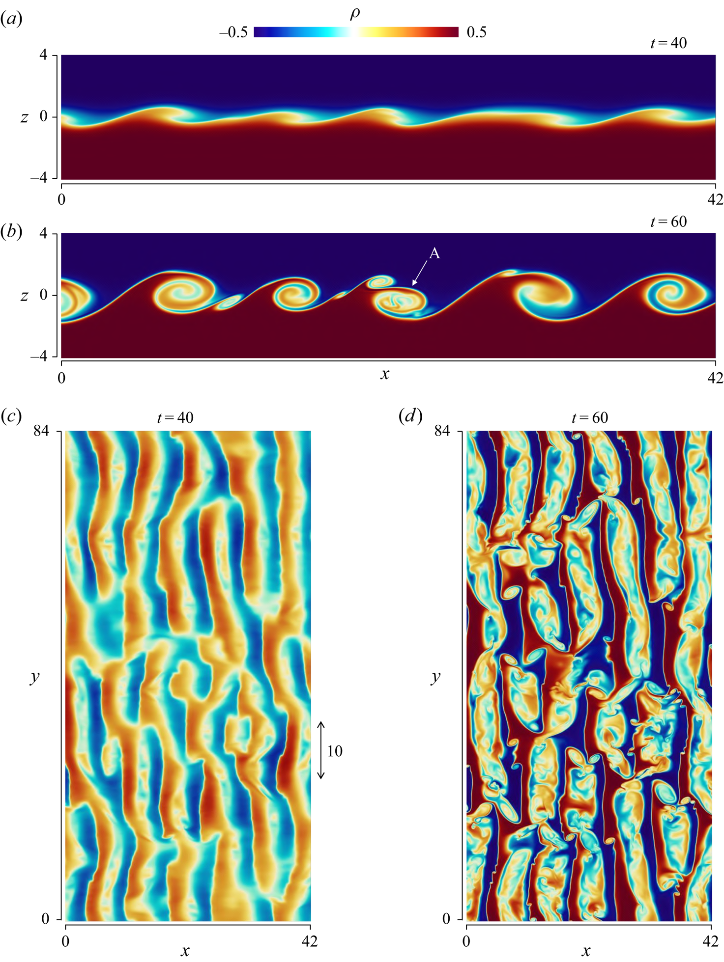
Figure 19. The same as figure 18 but for run 1: (a,b) an  $x$–
$x$– $z$ plane; (c,d) the horizontal plane at $z=0$. Profiles (a,c) are taken at $t=40$ while (b,d) are at $t=60$.
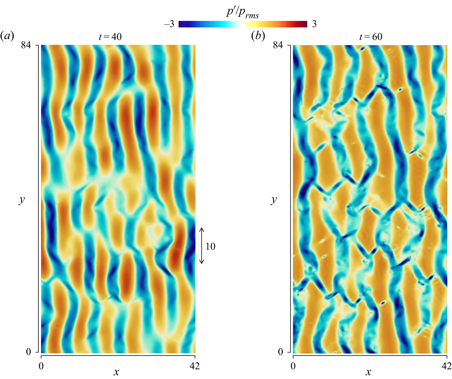
Figure 20. Pressure fluctuations  $p'=p-\langle p\rangle$ normalized by the r.m.s. fluctuations $p_{rms}$ on the horizontal plane at $z=0$ in run 1: (a) $t=40$; (b) $t=60$. The same region is visualized as in figure 19.
We also examine the effect of the domain size on the statistics of velocity and density. Figure 21(a) shows the temporal evolution of the shear layer thickness  $\delta _u$ and the momentum thickness $I_u=\int _{-L_z/2}^{L_z/2}(1- 4\langle u\rangle ^2)\,\textrm {d}z$ defined in Smyth & Moum (Reference Smyth and Moum2000b). The shear layer thickness after $t=100$ is smaller in run 7 than in run 1, and the shear layer growth is also influenced by the domain size. In run 1, $I_u$ keeps increasing with $t$. However, $I_u$ in run 7 tends to be constant for $100 \lesssim t \lesssim 130$ then slowly increases again. Similarly, the previous DNS whose domain size is as small as run 7 also found that $I_u$ ceases to grow after the rapid initial increase due to the instability and then it slowly increases at a late time (Smyth & Moum Reference Smyth and Moum2000b).
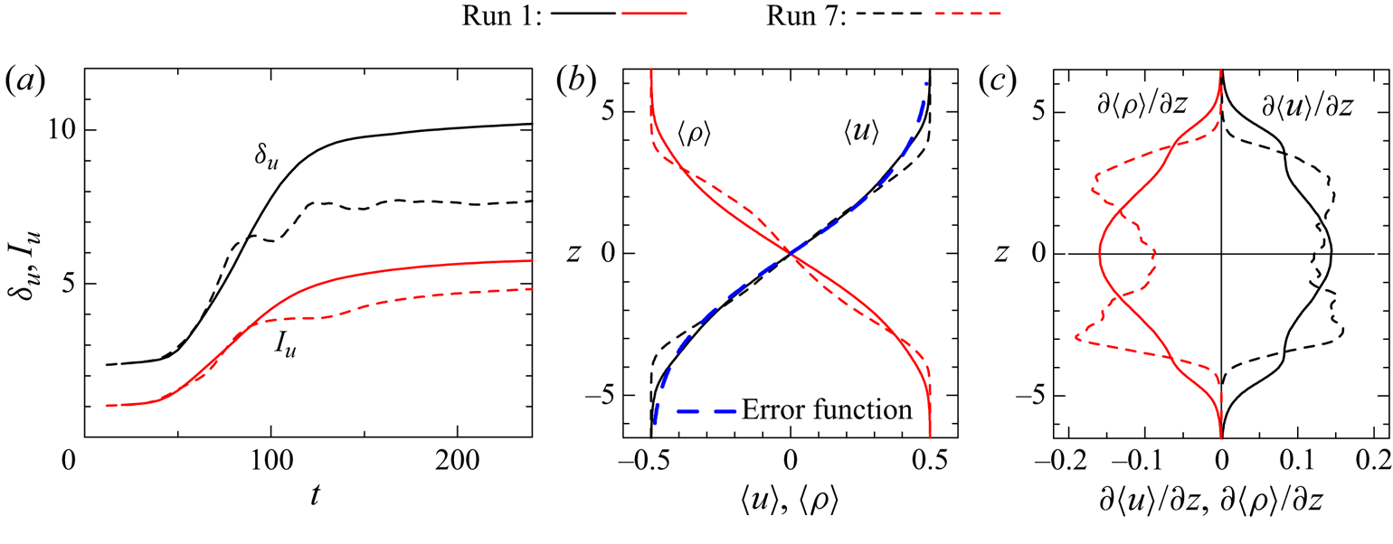
Figure 21. (a) Shear layer thickness  $\delta _u$ and momentum thickness $I_u$. Vertical profiles of (b) mean streamwise velocity $\langle u\rangle$ and density $\langle \rho \rangle$, and (c) mean velocity and density gradients, $\partial \langle u\rangle /\partial z$ and $\partial \langle \rho \rangle /\partial z$, at $t=240$.
Figure 21(b) compares the vertical profiles of  $\langle u \rangle$ and $\langle \rho \rangle$ at $t=240$ in runs 1 and 7 while figure 21(c) shows $\partial \langle u \rangle /\partial z$ and $\partial \langle \rho \rangle /\partial z$. Both $\langle u \rangle$ and $\langle \rho \rangle$ smoothly vary with $z$ in run 1, and the mean velocity and density gradients become the largest at $z=0$. In experiments by Champagne, Pao & Wygnanski (Reference Champagne, Pao and Wygnanski1976) the mean streamwise velocity profile in a non-stratified turbulent mixing layer is well approximated by an error function $\mathrm {erf}(X)$ as $\langle u \rangle =0.5\,\mathrm {erf}(z/\delta _e)$ (Pope Reference Pope2000). Figure 21(b) also shows $\langle u \rangle =0.5\,\mathrm {erf}(z/\delta _e)$ with $\delta _e=3.8$ and the error function is a good approximation of $\langle u \rangle$ in run 1. On the other hand, the inflection points of $\langle \rho \rangle$ appear not only at $z=0$ but also at $|z|\approx 3$ in run 7. Therefore, $\partial \langle \rho \rangle /\partial z$ has peaks at $|z|\approx 3$. Similarly, the largest value of $\partial \langle u \rangle /\partial z$ appears at $|z|\approx 3$ in run 7. Consistently, previous studies with small domains also reported the mean velocity and density profiles similar to run 7 (Smyth & Moum Reference Smyth and Moum2000a; Mashayek & Peltier Reference Mashayek and Peltier2013; VanDine et al. Reference VanDine, Pham and Sarkar2021). These previous DNS are different from our DNS in terms of ${Re}$ and initial velocity fluctuations, and the domain size effect may also be different in these studies. However, the largest gradient of $\langle u \rangle$ and $\langle \rho \rangle$ appears at $z=0$ even in run 5 (LES) with $({Re}, Ri)=(40\,000,0.06)$, indicating that the domain size effect is similar even at higher ${Re}$ than 2000. As also discussed below, the domain size effect found in this study is similar to that in DNS of a spatially developing turbulent mixing layer, where the initial (inflow) velocity fluctuations and the initial Reynolds number are also different from the present simulations.
Figure 22 presents the temporal variations of various statistics. Plots (a–d) compare the velocity and density variances in runs 1 and 7 and DNS results by Watanabe et al. (Reference Watanabe, Riley and Nagata2017), where DNS of the stratified shear layer was performed for the same values of ( ${Re},Ri,Pr$) with $(L_x,L_y,L_z)=(48,28,80)$. The variances evolve with time quite differently in run 7 compared with other DNS. One of the most important differences is in the growth of $\langle v'^2\rangle$, which is significantly delayed in run 7. This can be explained by the quasi-two-dimensional roller vortices that persist for a long time because the periodic boundary condition with small $L_y$ inhibits the three-dimensionalization of the vortices as discussed above. Direct numerical simulation by Watanabe et al. (Reference Watanabe, Riley and Nagata2017) predicts well the initial growth of $\langle v'^2\rangle$, and $(L_x,L_y,L_z)=(48,28,80)$ is large enough to prevent the unphysical effects of the domain size on the turbulent transition. However, this does not mean that the domain size is sufficiently large at a late time as $(L_x, L_y, L_z)=(48,28,80)$ is too small for the ELSS to naturally develop. Figure 22(e) compares the turbulent kinetic energy dissipation rate $\varepsilon ^{(k)}$ at $z=0$ between runs 1 and 7, where the difference arising from the domain size is clear. Figure 22(f) presents the production $P_k=\int (-\langle u'w'\rangle \partial \langle u\rangle /\partial z)\,\textrm {d}z$ and buoyancy flux $B_k=\int (-Ri\langle \rho 'w'\rangle )\,\textrm {d}z$ of the vertically integrated turbulent kinetic energy budget, where the integral is taken from $z=-L_z/2$ to $L_z/2$. In run 1, $P_k$ peaks at $t\approx 80$ and decreases with time while $B_k$ also tends to decrease after the turbulent transition. Very different behaviours of these terms are found in run 7: $P_k$ exhibits two distinct peaks at $t\approx 70$ and 140 and $B_k$ becomes positive after the largest negative peak at $t\approx 80$. Similar temporal oscillations of $P_k$ and $B_k$ were reported by VanDine et al. (Reference VanDine, Pham and Sarkar2021), where the domain size is as small as in run 7.
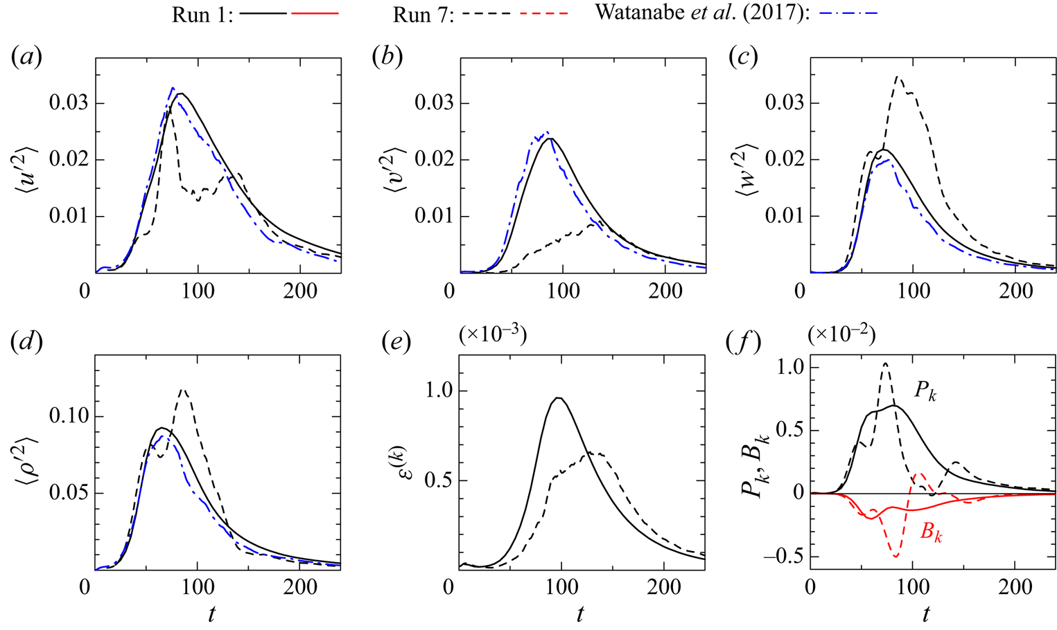
Figure 22. Temporal evolutions of statistics: variances of (a) streamwise velocity, (b) spanwise velocity, (c) vertical velocity, (d) density, (e) turbulent kinetic energy dissipation rate, (f) vertically integrated production and buoyancy flux of the turbulent kinetic energy budget. The results in (a–e) are taken at  $z=0$. In (a–d) the present DNS results are compared with DNS in Watanabe et al. (Reference Watanabe, Riley and Nagata2017) with $(L_x,L_y,L_z)=(48,28,80)$.
These results prove that the finite domain size has significant influences on the stably stratified shear layer if the domain size is as small as  $(L_x, L_y, L_z)=(14, 4, 50)$. It should be noted that some previous studies tested the sensitivity of DNS to the domain size. For example, Mashayek & Peltier (Reference Mashayek and Peltier2013) confirmed that doubling of the spanwise domain size from $L_y=2$ to 4 did not affect the flow development. However, the results presented in this appendix indicate that even in the DNS with $L_y=4$ used for their validation, the domain size was not large enough to prevent the unphysical effects of the periodic boundary conditions since the spanwise length of the meandering vortices in figure 20 is longer than 10. Thus, the findings based on the previous DNS with a small domain may need to be carefully re-examined in future works.
Finally, it should also be noted that most of these influences of the domain size are consistent with the confinement effects observed in spatially developing, non-stratified turbulent mixing layers. It was shown that the quasi-two-dimensional primary roller vortices persist for a longer time when the spanwise domain is not large enough to prevent the confinement effects (Biancofiore Reference Biancofiore2014; McMullan Reference McMullan2015). Flow visualization in their studies also confirmed that the interactions between meandering roller vortices lead to a fast transition to three-dimensional turbulence as also observed in this study. Furthermore, they also showed that the confinement effects in the spanwise direction suppress the growth of the momentum thickness. Similarly, the momentum thickness in run 7 is smaller than in run 1 in figure 21(a). McMullan (Reference McMullan2015) showed that this spanwise confinement effect on the mixing layer growth occurs for  $L_y/I_u<2.5$. Here, the definition of $I_u$ in this study follows Smyth & Moum (Reference Smyth and Moum2000b) while McMullan (Reference McMullan2015) defined it as $\int _{-L_z/2}^{L_z/2}(0.25- \langle u\rangle ^2)\,\textrm {d}z$, which yields 1/4 times smaller values of $I_u$ of Smyth & Moum (Reference Smyth and Moum2000b). Therefore, criterion 2.5 is different by a factor of 1/4 from that given in McMullan (Reference McMullan2015). In this study, all DNS and LES except for run 7 satisfy $L_y/I_u>2.5$, where the smallest value of $L_y/I_u$ is 4 obtained at $t=320$ in run 3 with $({Re},Ri)=(40\,000,0)$. On the other hand, run 7 with $L_y=4$ does not satisfy $L_y/I_u>2.5$ after $t=50$, and the shear layer development is strongly influenced by the spanwise confinement. The criterion $L_y/I_u>2.5$ was obtained for spatially developing, non-stratified turbulent mixing layers, and may not be the exact value for the occurrence of the spanwise confinement in the temporally evolving, stratified shear layer. At least, it suggests that $L_y<10$ is too small for the shear layer to naturally develop without the confinement effect.


