


1. Introduction
In the Rayleigh–Stokes problem, an initially stationary and unbounded Newtonian fluid lying above a horizontal plate is set into motion by the sudden in-plane motion of the plate. This problem was first proposed and solved by Stokes (Reference Stokes1851) and later expounded by Rayleigh (Reference Rayleigh1911); it is variably called ‘Stokes’ first problem’, the ‘Rayleigh problem’ or the ‘Rayleigh–Stokes problem’ in the literature; we use the latter. For plate motion with constant velocity in its plane  $U_0 \hat {\boldsymbol {x}}$, where $\hat {\boldsymbol {x}}$ is the basis vector in the Cartesian $x$-direction, the resulting velocity field of the fluid, $u(y, t)\,\hat {\boldsymbol {x}}$, satisfies the momentum equation
 \begin{equation} {}{\rho\,\frac{\partial u}{\partial t} = \frac{\partial \tau}{\partial y}}, \end{equation}
where  $y$ is the Cartesian coordinate normal to the plate, $t$ is time, $\tau$ is the $xy$ (shear) component of the Cauchy stress tensor, and $\rho$ is the density. For the semi-infinite (unbounded) region of a Newtonian fluid, the velocity disturbance propagates into the fluid in a self-similar fashion, moving away from the plate with a $\sqrt {t}$ time dependence (figure 1a):
 \begin{equation} u \equiv u_{N,\infty} = U_0 \operatorname{erfc} \left(\frac{y}{2\sqrt{\nu t}} \right), \end{equation}
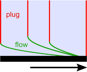
where the first subscript,  $N$, denotes the flow of a Newtonian fluid, while the second subscript specifies the spatial extent of the fluid normal to the plate. Analytical solution for a finite (bounded) region of Newtonian fluid with a free surface is also obtained readily (Liu Reference Liu2008); the free surface is initially stationary and accelerates gradually until its velocity converges with that of the plate (figure 1b).

Figure 1. The Rayleigh–Stokes problem for a Newtonian fluid and a Bingham material. The solid plate under the material moves suddenly from rest, and in its plane, with constant velocity  $U_0 \hat {\boldsymbol {x}}$. Curves show the evolution of the velocity field parallel to the plate, as a function of time $t$. (a) A semi-infinite region of Newtonian fluid. (b) A finite region of Newtonian fluid with a free surface. (c) A finite region of Bingham material with a free surface.
While these simple solutions provide significant insight into momentum diffusion through viscous boundary layers, many materials of environmental, industrial and biological importance do not obey a Newtonian constitutive law. An important class, known as yield-stress (or viscoplastic) materials, are characterised by constitutive laws where a sufficiently large stress must be applied to the material before it can flow. A simple model introduced by Bingham (Reference Bingham1916) states that the material is rigid below a critical state of stress, above which the material behaves as a Newtonian fluid. For a general unidirectional plane flow of velocity,  $u(y, t)\,\hat {\boldsymbol {x}}$, these ‘Bingham’ materials obey the constitutive equation (Bingham Reference Bingham1922)
 $$\begin{gather} \frac{\partial u}{\partial y} = 0 \quad \text{for}\ |\tau| < \tau_Y, \end{gather}$$
 $$\begin{gather}\tau=\mu\frac{\partial u}{\partial y} + \tau_Y \operatorname{sgn}\left( \frac{\partial u}{\partial y}\right) \quad \text{for}\ |\tau| \ge \tau_Y, \end{gather}$$
where  $\tau _Y$ is the shear yield stress and $\mu$ is the shear viscosity. This seemingly simple constitutive model gives rise to rich flow behaviour and applications not possible with Newtonian fluids.
A key feature of a viscoplastic flow is the presence of a ‘yield surface’, i.e. a surface that separates a yielded (fluid-like) region and a rigid region of the material (Balmforth, Frigaard & Ovarlez Reference Balmforth, Frigaard and Ovarlez2014); any particular flow may contain a number of yield surfaces. These surfaces are often time-dependent and can be created or destroyed depending on the flow in question (Huilgol Reference Huilgol2004).
In many industrial applications, viscoplastic boundary layers play an important role. For example, Peixinho et al. (Reference Peixinho, Nouar, Desaubry and Théron2005) studied the flow of both Newtonian fluids and yield-stress materials through pipes. They found that the presence of a yield stress stabilises the flow, thus higher Reynolds numbers can be achieved before the onset of turbulence. Moreover, it has been reported that Poiseuille flow of a viscoplastic material comes to rest in finite time when the forcing is removed (Huilgol, Mena & Piau Reference Huilgol, Mena and Piau2002; Chatzimina et al. Reference Chatzimina, Georgiou, Argyropaidas, Mitsoulis and Huilgol2005). Transient viscoplastic and bi-viscous flows in pipes, with a time-dependent pressure gradient or wall velocity, have also been well studied, with detailed mathematical solutions developed for the evolution of the yield surface (Safronchik Reference Safronchik1959a, Reference Safronchik1960; Comparini Reference Comparini1992; Burgess & Wilson Reference Burgess and Wilson1997). The flow exterior to a cylinder with general applied angular velocity has also been considered (Safronchik Reference Safronchik1959b). These flows do not have a free surface, which, as we show here, exerts a leading-order effect on the flow physics.
Applications also arise in natural processes, where a Bingham material has been employed to model the effect of shallow water waves on a muddy sea-bed (Mei & Liu Reference Mei and Liu1987). The key finding from these works is that the viscoplastic sea-bed acts as a damper to the waves (Ng Reference Ng2000; Chan & Liu Reference Chan and Liu2009; Roustaei, Gosselin & Frigaard Reference Roustaei, Gosselin and Frigaard2015). This problem forms a complementary view to Rayleigh–Stokes type problems because the free surface of the material, rather than its solid base, is disturbed.
For the semi-infinite (unbounded) Rayleigh–Stokes problem, replacing the Newtonian fluid with a Bingham material does not alter the velocity field (Pascal Reference Pascal1989), which is identical to (1.2). The key difference is that the shear stress in a Bingham material is offset from its Newtonian counterpart by the yield stress, throughout the flow domain, i.e. the magnitude of the shear stress is held above the yield stress,
 \begin{equation} \tau = \mu\,\frac{\partial u_{N,\infty}}{\partial y} -\tau_Y, \end{equation}
for which  $\partial u_{N,\infty }/\partial y <0$; see (1.2). This means that the shear stress at the solid plate approaches a constant value $-\tau _{Y}$ as $t\rightarrow \infty$, unlike Newtonian flow where the shear stress approaches zero. That is, a greater shear stress must be applied to the plate to move an unbounded region of Bingham material relative to its Newtonian counterpart. Equation (1.4) shows that the Bingham material is always yielded. Hence it never contains rigid regions or a yield surface – a key characteristic that, as discussed above, leads to much of the interesting behaviour associated with yield-stress materials. The closely related ‘shear-driven’ Rayleigh–Stokes problem for an unbounded region of Bingham material, i.e. constant shear stress applied by the plate, also admits an analytical solution for the velocity field identical to its Newtonian counterpart (Duffy, Pritchard & Wilson Reference Duffy, Pritchard and Wilson2014), provided that the applied stress at the plate exceeds the yield stress (see also Sekimoto Reference Sekimoto1991). No motion occurs if the applied stress is less than the material's yield stress.
Non-Newtonian versions of Stokes’ second problem, where the plate oscillates periodically in time (rather than moving abruptly with constant velocity), have drawn more attention than the first problem. Balmforth, Forterre & Pouliquen (Reference Balmforth, Forterre and Pouliquen2009) considered the role of yield stress in the second problem for a Bingham material of finite height, bounded by a free surface. Their numerical results showed that isolated regions of yielded material, separated by rigid regions, move periodically from the plate to the free surface. The second problem, with power-law and thixotropic materials in semi-infinite and unbounded domains, has also been explored (Pritchard, McArdle & Wilson Reference Pritchard, McArdle and Wilson2011; McArdle, Pritchard & Wilson Reference McArdle, Pritchard and Wilson2012). For shear-thickening materials, these studies show that the velocity vanishes beyond a finite distance from the plate, in contrast to the Newtonian case. Stokes’ second problem differs from the first problem because the spatial extent of momentum diffusion in the former is controlled by the plate oscillation time scale. While the Laplace transform links these two problems for a Newtonian fluid (Stokes Reference Stokes1851), flow of a Bingham material is an intrinsically nonlinear process that alters the flow physics (and analyses) of the first and second problems.
We consider the Rayleigh–Stokes problem for a Bingham material of finite height with a free surface, whose behaviour differs considerably from that of a semi-infinite region or a layer bounded by no-slip boundaries (discussed above). The velocity gradient is singular initially at the solid plate due to its sudden motion, ensuring that the yield surface propagates from the plate into the material immediately following start-up. The shear stress at the free surface vanishes, ensuring that the material is rigid in its vicinity. Because the material is always rigid near the free surface and yields initially near the plate, a yield surface exists that can evolve in time. Importantly, the Rayleigh–Stokes problem for a Bingham material of finite height is yet to be reported and its fluid physics explored. This is the focus of the present study, which includes both numerical and analytical solutions. We also show how the results generalise to other related materials, in particular for a general Herschel–Bulkley constitutive law that exhibits either shear-thinning or shear-thickening post-yield behaviour.
The paper is structured as follows: The theoretical foundation for the Rayleigh–Stokes problem involving a Bingham material of finite height with a free surface is formulated in § 2, and illustrated in figure 1(c). We non-dimensionalise the problem, which identifies the Bingham number  $B$, defining the magnitude of the yield stress relative to the viscous shear stress generated by the plate. Numerical results as a function of Bingham number are reported in § 2.1. The physical mechanisms driving the flow, reported in § 2.1, are explored in § 3. This begins by identifying the general properties of the rigid and yield regions of the material in §§ 3.1 and 3.2, respectively. An upper bound for the ‘collision time’, at which the entire material becomes rigid, is derived in § 3.3. In § 3.4, we show that at early time, the yield surface does not travel far from the plate and the material behaves as if it were unbounded; the Newtonian solution for the velocity field applies. In § 3.5, the Newtonian solution is deployed to analyse the problem for small $B$. This describes the evolution of the yield surface and the collision time. Immediately prior to the collision time, the material is almost entirely rigid. In § 3.6, we use this property to prove that the velocity field is self-similar in this regime. The dynamics at large Bingham number is explored in § 3.7, for which a rescaling reduces the motion to a universal system defining an unusual type of Stefan problem. A comparison of the dynamics for small and large $B$ is reported in § 3.8, and approximate formulas are given in § 3.9 that may be useful in practice. In § 4, we propose a rheometer that uses the dynamics of the free surface to study the existence of the yield stress and measure its value. Each result in the paper can be extended to more complicated viscoplastic constitutive laws. Throughout, we highlight where the analysis for a Bingham material applies either to any viscoplastic material or to a general Herschel–Bulkley material. The mathematical details are relegated to Appendix A, where we itemize the generalisation of each section of the main text. Importantly, we find that the flow physics in all cases is dominated by the yield stress. Concluding remarks are provided in § 5, with details of the numerical methods used in this study given in Appendix B.
2. Theoretical formulation
We consider a Bingham material that is initially at rest, bounded by a solid plate at  $y=0$ and a free surface at $y=H$; see figure 1(c). The solid plate is suddenly set into motion at time $t=0$, with constant velocity $U_0 \hat {\boldsymbol {x}}$. This motion generates a unidirectional and incompressible flow of constant density and velocity $u(y,t)\,\hat {\boldsymbol {x}}$. The governing equations for the resulting flow are provided by (1.1) and (1.3), with initial and boundary conditions
 \begin{equation} u(y, 0) = 0,\quad u(0, t) = U_0,\quad \tau(H, t) = 0, \end{equation}
corresponding to no initial flow, no-slip at the solid plate, and no shear stress at the free surface, respectively.
The  $y$-coordinate is scaled by the height of the material, $H$; time $t$ is non-dimensionalised by the time scale for momentum diffusion, $H^{2}/\nu$; the shear stress $\tau$ is scaled by $\mu U_0/H$ for consistency with the chosen time scale; and the material velocity $u$ is scaled by that of the plate, $U_0$. In their corresponding dimensionless forms, (1.1) and (1.3) become
 \begin{equation} \frac{\partial u}{\partial t} = \frac{\partial \tau}{\partial y} \end{equation}
and
 $$\begin{gather} \frac{\partial u}{\partial y} = 0 \quad \text{for}\ |\tau| < B, \end{gather}$$
 $$\begin{gather}\tau=\frac{\partial u}{\partial y} + B \operatorname{sgn}\left( \frac{\partial u}{\partial y} \right) \quad \text{for}\ |\tau| \ge B, \end{gather}$$
where the Bingham number is
 \begin{equation} B \equiv \frac{\tau_Y H}{\mu U_0}, \end{equation}
defining the ratio of the yield to viscous stresses. The initial and boundary conditions in (2.1a–c) become
 \begin{equation} u(y, 0) = 0,\quad u(0, t) = 1,\quad \tau(1, t) = 0. \end{equation}
All variables will henceforth refer to their dimensionless quantities, unless indicated otherwise.
While our analysis focuses on a Bingham material, it is straightforward to extend each of the results to a general Herschel–Bulkley material and in some cases to any viscoplastic material; the details of this are given in Appendix A. The flows of all such materials are similar because they share the same key ingredient: a yield stress.
2.1. Numerical solutions
We commence our discussion of the Rayleigh–Stokes problem for a layer of Bingham material (figure 1c) by presenting numerical solutions of the governing equations spanning the small, intermediate and large Bingham number regimes. This is achieved by solving numerically (2.2)–(2.5a–c) directly for the shear stress  $\tau$ throughout the domain $0 \le y \le 1$, using a semi-implicit method. Acceleration of the material, and hence its velocity field $u$, then follow from (2.3). The details of the numerical method, including its extension to a general Herschel–Bulkley material, are given in § B.1 of Appendix B.
Results for the velocity  $u$ and shear stress $\tau$ of the material for $B = 20, 1, 1/20$ are shown in figure 2, in the form of space–time colour maps. We denote the position of the yield surface, where $|\tau |=B$, by $y=Y(t)$; the material is yielded within $0\le y\le Y(t)$ and rigid for $Y(t)< y\le 1$. The yield surfaces in figure 2 are indicated by the red curves.


In all cases, we observe that the entire layer of Bingham material comes to move rigidly with the solid plate in finite time, denoted  $t= t_f\ (> 0)$ – a general feature for $B>0$. Numerical results for this ‘collision time’ are given in figure 3(a), which corresponds to collision of the yield surface with the plate; see figure 2. This behaviour differs from the singular limit of a Newtonian fluid, i.e. $B=0$ (figure 1b), where the fluid never moves rigidly, but rather asymptotically approaches rigid body motion as time evolves. Moreover, the finite collision time required to reach rigid body motion throughout the Bingham material decreases with increasing $B$; see figure 3(a). The spatial extent of the yield surface also decreases as $B$ increases, i.e. less of the material yields before complete rigid body motion; cf. figures 2(a) and 2(e), quantified in figure 3(b).

Figure 3. (a) Collision time  $t = t_f$ for a Bingham material to move entirely as a rigid body with the plate velocity $u = 1$. (b) Maximum height of the yield surface, $Y_{{max}}$, as a function of the Bingham number $B$. Numerical results as per § 2.1.
These observations of the material can be understood by noting that an increase in  $B$ can be achieved by increasing the yield stress while holding all other parameters constant. For very high yield stress, virtually none of the material yields before moving rigidly and almost instantly with the plate, i.e. the material behaves as a rigid solid block. In contrast, for very small yield stress, nearly all the material yields almost instantly after start-up, i.e. it behaves initially as a Newtonian fluid. As the material accelerates, the shear stress then decreases, with the material eventually recovering its solid-like behaviour prior to start-up.
It is clear from figure 2 that the dynamics of the yield surface controls the material motion, and the dynamics differs for small and large  $B$. The physical mechanisms and details of this dependency – features of the yield curve and its effect on the overall material dynamics – are investigated in the following sections.
3. Physical mechanisms
In this section, we explore the physical mechanisms driving the dynamics of a layer of Bingham material whose lower surface is suddenly set into motion. This includes using an alternative analysis to that above, which enables direct calculation of both the velocity field and yield surface; in § 2.1, the stress field was calculated directly. This alternative analysis facilitates the deployment of both analytical and numerical methods.
Due to sudden motion of the solid plate at  $t=0$, i.e. infinite acceleration, the shear stress at the plate initially exceeds the yield stress. Because material away from the solid plate cannot move abruptly, it follows that the yield surface must originate at the plate. Following start-up, the yield surface moves away from the plate before returning to the plate in finite time, after which the entire material is rigid; see figure 2 (cf. Ancey & Bates Reference Ancey and Bates2017).
3.1. Rigid region
In the rigid region above the yield surface, i.e.  $Y(t)< y\le 1$, the velocity field of the material is constant:
 \begin{equation} u \equiv u_R(t), \end{equation}
where the subscript  $R$ denotes the rigid material and is used throughout for clarity. At the position of the yield surface, the shear stress is $\tau =-B$, hence the material is on the verge of flowing; see (2.3). Note that the shear stress $\tau$ is always non-positive owing to the sign of the velocity gradient and the chosen Cartesian coordinate system; see figure 1. In this rigid region, we differentiate the momentum equation (2.2) with respect to $y$ to obtain
 \begin{equation} \frac{\partial^{2} \tau_R}{\partial y^{2}} =0 . \end{equation}
This shows that the shear stress in the rigid region increases linearly from  $\tau _R=-B$ at $y=Y(t)$, to $\tau _R=0$ at the free surface $y=1$. This result applies to any viscoplastic material because the rigid region arises from the existence of the yield stress, and is independent of the constitutive law when the material yields. For further details, see Appendix A.
3.2. Yielded region
In the yielded region, i.e.  $0\le y\le Y(t)$, the magnitude of the shear stress $\tau$ exceeds the yield stress, and the momentum equation (2.2) reduces to its Newtonian form,
 \begin{equation} \frac{\partial u}{\partial t} = \frac{\partial^{2} u}{\partial y^{2}}, \end{equation}
which is supplemented by three boundary conditions. First, after start-up ( $t>0$), the material velocity matches that of the plate,
 \begin{equation} u(0, t) = 1, \end{equation}
while second, at the yield surface,
 \begin{equation} \left. \frac{\partial u}{\partial y} \right|_{y=Y(t)}=0, \end{equation}
because the shear stress must be continuous at the yield surface.
The third boundary condition (Balmforth et al. Reference Balmforth, Forterre and Pouliquen2009) is obtained by first integrating (2.2) over the rigid region  $Y(t) < y \le 1$, and using the properties that $\tau _R=-B$ at $y=Y(t)$, and $\tau _R=0$ at $y=1$. Noting that the velocity is continuous at the yield surface, i.e. $u(Y(t), t) = u_R(t)$, then gives the required result (see also Sekimoto Reference Sekimoto1993):
 \begin{equation} (1-Y) \left.\frac{\partial u}{\partial t} \right|_{y=Y(t)} = (1-Y)\,\frac{\partial u_R}{\partial t}= B. \end{equation}
Equation (3.6) is simply a restatement of Newton's second law, that the shear stress  $\tau = \tau _R=-B$ at the yield surface accelerates the rigid region above it of thickness $1-Y$. Since $B>0$, (3.6) establishes that acceleration of the rigid region is strictly non-negative. The three boundary conditions (3.4), (3.5) and (3.6) apply to the yielded region for any viscoplastic material, although the governing equation (3.3) in the yielded region will generally be nonlinear (for further details, see Appendix A).
Rewriting (3.6) as
 \begin{equation} Y = 1- \frac{B}{\partial u_R / \partial t} \end{equation}
shows that  $Y(t)$ is a monotonically increasing function of $\partial u_R/\partial t$. That is, maximum $Y$ corresponds to maximum acceleration of the rigid region. This is because the shear stress – and hence driving force – is constant at the yield surface $y=Y(t)$, and given by $\tau =-B$. Plots showing the time evolution of $Y(t)$ and $\partial u_R/\partial t$, for $B=1$ and 5, are given in figure 4, obtained using the numerical results in § 2.1.

Figure 4. Acceleration  $\partial u_R / \partial t$ of the rigid region adjacent to the free surface (black curves, left-hand axes), and the location of the yield surface $Y(t)$ (red dashed curves, right-hand axes), for (a) $B=0$ (Newtonian fluid), for which there is no yield surface, (b) a Bingham material with $B=1$, and (c) a Bingham material with $B=5$. Numerical results as per § 2.1. The dotted horizontal specifies the minimum acceleration, i.e. $\partial u_R / \partial t = B$, as per (3.8). Numerical results for the acceleration exclude the zero acceleration conditions specified at the end points $t=0$ and $t_f$; see § B.2 of Appendix B.
To explain this observed transient evolution of the location of the yield surface, we first explore how the rigid material near the free surface accelerates. Immediately after start-up, i.e. at ‘early time’, the free surface accelerates at a growing rate as momentum diffuses out from the plate where the material has yielded. Later, the material moves at speeds comparable to the plate, which reduces the velocity gradients. The shear stress at the plate, and hence the acceleration of the material, subsequently decreases with time. This behaviour is shown by the black solid curves in figure 4, which give the acceleration of the rigid region, and hence the free surface. The location of the yield surface for  $B=1$ and $B=5$ (red dashed curves in figure 4) moves monotonically with the acceleration of the free surface; the yield curve has a turning point owing to the change in the rate of acceleration of the free surface.
Equation (3.7) also demonstrates that for small  $B$, the yield surface is close to the free surface (i.e. $Y\approx 1$) when the acceleration of the rigid region is not small, i.e. much larger than $B$. This occurs very shortly after initiation of the motion; see figures 2(e, f). However, the acceleration is subsequently much slower to decay than for a material with larger yield stress; see figure 4(a). Hence for small $B$, the time scale for relaxation to the fully rigid motion is longer. These effects are discussed in more detail in §§ 3.4 and 3.5.
3.3. Collision time
Equation (3.6) is derived assuming that a yield curve exists where  $\tau = - B$, i.e. a yielded region occurs below the yield surface. From (3.6), it then follows that acceleration of the rigid region near the free surface must satisfy
 \begin{equation} \frac{\partial u_R}{\partial t} \geq B \end{equation}
when a yielded region exists, which is evident in figures 4(b,c). This behaviour contrasts with flow of a Newtonian fluid for which the shear stress at the plate (and hence the material acceleration) approaches but never reaches zero as time increases, for  $t \gg 1$.
Evidently, for a Bingham material, a time must be reached where (3.8) is violated, otherwise the material would accelerate ad infinitum. This corresponds to the collision time  $t = t_f$ (defined above), where the yield surface collides with the solid plate and extinguishes the yield region. At and after this time, shear stress at the plate, and throughout the material, drops to zero, and the entire material moves as a rigid body in concert with the plate.
An upper bound for this collision time can be derived. Integrating the inequality in (3.8) with respect to time  $t$, while noting that the rigid material is initially at rest, i.e. $u_R |_{t=0}=0$, and cannot exceed the plate velocity, i.e. $u_R \le 1$, gives the required result:
 \begin{equation} t_f \leq \frac{1}{B}. \end{equation}
Equation (3.9) is shown as a dashed blue curve in figure 3(a), where it indeed provides an upper bound to the full numerical solution for all  $B$.
$B$.
For large  $B$, the yield curve stays close to the solid plate at all times, i.e. $Y \ll 1$, and almost the entire material region remains rigid. That is, the inequalities in (3.8) and (3.9) become equalities as $B \rightarrow \infty$, which is evident in the comparison provided in figure 3(a).
The results for the bound on the rigid acceleration, the bound on the collision time, and the collision time for large  $B$, apply generally to any viscoplastic material.
3.4. Early time
At early time, immediately following start-up, the material dynamics possess two key properties: (i) the velocity field is non-negligible only in the immediate neighbourhood of the plate; and (ii) the yield surface remains close to the plate (Burgess & Wilson Reference Burgess and Wilson1997). These properties imply that the free surface cannot yet influence the material dynamics. That is, the velocity field for start-up of a semi-infinite (unbounded) region – identical to that of Newtonian flow, (1.2) – applies in the yielded region close to the plate. In dimensionless form, (1.2) becomes
 \begin{equation} u_{N,\infty} = \operatorname{erfc} \left(\frac{y}{2 \sqrt{t}}\right). \end{equation}
Also, provided that the yield curve  $Y(t)$ grows faster than $\sqrt {t}$, which we show a posteriori, $\partial u_{N,\infty }/\partial y \sim 0$ at $y=Y(t)$ for early time. In other words, the yield surface moves more quickly than transport due to momentum diffusion, which is evident in the numerical results of figure 2. Since $Y\ll 1$, the boundary condition at the yield surface in (3.6) becomes
 \begin{equation} \frac{\partial u}{\partial t} = B \quad \text{for}\ y=Y(t), \end{equation}
which can be integrated by noting that the yield surface originates from the plate, i.e.  $Y(0) = 0$, to give
 \begin{equation} u ( Y(t), t ) = B t . \end{equation}
Substituting (3.10) into (3.12) gives the evolution equation for the yield surface (for early time):
 \begin{equation} \operatorname{erfc} \left( \frac{Y}{2 \sqrt{t}}\right)= B t, \end{equation}
which shows that the appropriate rescalings for early time are  $t \sim 1/B$ and $Y \sim 1/\sqrt {B}$. Defining
 \begin{equation} \bar{t} = Bt, \quad \bar{y} = \sqrt{B} y,\quad \bar{Y} = \sqrt{B} Y, \end{equation}
then transforms the evolution equation (3.13) into one that is independent of  $B$:
$B$:
 \begin{equation} \bar{Y} = 2\sqrt{\bar{t}} \operatorname{erfc}^{{-}1} \bar{t}. \end{equation}
This prediction is compared to the numerical results for the yield surface evolution in figure 5(a) for a range of values of  $B$.
$B$.

Figure 5. Location of the yield surface  $Y$ at early times, for $B=1/25, 1/5, 1, 5, 25$. Accurate numerical results for arbitrary $B$, as per § 2.1 (solid black curves). (a) Data rescaled for small time as per (3.14a–c). Asymptotic solution is (3.15) (red dashed curve). (b) Data not rescaled. Improved asymptotic solution is (3.23) (red dot-dashed curves). The early time condition (3.22) for $B = 25$ is violated over the time duration shown.
For small  $\bar {t}$, (3.15) yields the asymptotic result
 \begin{equation} \bar{Y} \sim 2 \sqrt{\bar{t}} \sqrt{ \frac{1}{2} \log \left(\frac{\dfrac{2}{{\rm \pi} \bar{t}^{2}}}{ \log\left( \dfrac{2}{{\rm \pi} \bar{t}^{2}} \right) } \right)}, \end{equation}
while the velocity field (3.10) diffuses away from the plate with the time dependence:
 \begin{equation} \bar{y}_{vel} \sim 2 \sqrt{\bar{t}}, \end{equation}
with the subscript ‘vel’ referring to the velocity field. Equations (3.16) and (3.17) then give
 \begin{equation} \lim_{t \rightarrow 0^{+}} \frac{\bar{y}_{vel}}{\bar{Y}} = \lim_{t \rightarrow 0^{+}} \frac{\bar{y}'_{vel}}{\bar{Y}'} = 0, \end{equation}
via L'Hopital's rule, where  $'$ refers to the time derivative. Consistency of (3.18) with the imposed assumption that the yield surface moves away from the plate at a much faster rate than the velocity field, just after start-up, confirms the validity of this assumption.
We also calculate the shear stress applied by the plate,  $\tau _{plate}$, to the material at early time, to ensure that the plate moves at constant velocity $U_0 \hat {\boldsymbol {x}}$. Substituting (3.10) into (1.4) (in its dimensionless form) gives the required result:
 \begin{equation} \tau_{plate} ={-} \left( \frac{1}{\sqrt{{\rm \pi} t}} + B \right). \end{equation}
3.4.1. Duration of the early time period
We next calculate the duration of the early time period. Equation (3.13) relies on two conditions. The first is that the velocity field in the rigid region (away from the plate), just after start-up, is close to zero, i.e.  $u_R \ll 1$. Because $u_R =Bt$ immediately following start-up, as established by (3.12), this small velocity condition in the rigid region is equivalent to
 \begin{equation} t \ll \frac{1}{B}. \end{equation}
Second, the yield surface remains close to the plate just after start-up, i.e.  $Y \ll 1$. Equation (3.16) implies that $Y \sim \sqrt {t}$, which then imposes a second constraint that
 \begin{equation} t \ll 1. \end{equation}
The conditions (3.20) and (3.21) are different when  $B\neq 1$. This indicates that the early-time regime is shorter for larger values of $B$, but its extent is independent of $B$ for small $B$. The intersection of (3.20) and (3.21) gives the required duration of the early time period:
 \begin{equation} t \ll \min \left( 1, \frac{1}{B} \right),\quad \text{`early time period'}. \end{equation}
 This highlights the different physical mechanisms at play in the small and large yield-stress regimes, i.e. small and large  $B$, respectively. Equation (3.22) gives $t \ll 1$ for small $B$, consistent with the velocity field and yield surface both being controlled by momentum diffusion; see the chosen (dimensional) time scale of $H^{2}/\nu$ in § 2. In contrast, for large $B$, the time scale is reduced by a factor of $B$, which corresponds dimensionally to $\rho U_0 H/ \tau _Y$. This time scale arises from acceleration of the rigid region above the yield surface, driven by its (constant) stress, $\tau _Y$, with momentum diffusion playing a negligible role.
3.4.2. Dynamics of the yield surface just after the early time period
Here, we calculate the yield surface position  $Y$ when it is no longer very close to the solid plate, but the velocity of the rigid region remains small; $u_R \ll 1$. This situation can arise because the yield surface moves away from the plate at a rate faster than that of the velocity disturbance (see § 3.4); it is irrelevant for large $B$ where the yield surface always stays close to the plate.
Since  $Y \ll 1$ no longer holds, we retain the $1-Y$ term in (3.6) to give the refined evolution equation for the yield surface:
 \begin{equation} \frac{(1-Y) Y}{2 \sqrt{\rm \pi} t^{3/2}} \exp\left( - \frac{Y^{2}}{4 t}\right) = B, \end{equation}
whose solution for  $Y$ is compared to the accurate numerical results for arbitrary $B$ (as per § 2.1) in figure 5(b).
For a general Herschel–Bulkley material, the results are qualitatively similar but with different scalings for the thickness of the yielded region. The time scale for the early-time behaviour is the same as for a Bingham material. For further details, see Appendix A.
3.5. Small Bingham number
For zero yield stress,  $B =0$, the velocity field is given by that for Newtonian flow, i.e. $u_N(y,t)$. Because flow occurs everywhere in a Newtonian fluid, the yield surface of a Bingham material with $B = 0$ will reside at its free surface, i.e. $Y = 1$. We use these Newtonian results in a regular perturbation expansion for small $B$:
$B$:
 \begin{equation} u(y,t)=u_N(y,t) + o(1),\quad Y(t)=1-B\,Y_1(t)+ o(B), \end{equation}
where  $Y_1$ is to be determined, while the velocity field for a Newtonian fluid of finite extent with a free surface, is
 \begin{equation} u_N(y,t)= 1 - \sum_{n=0}^{\infty} \frac{4}{(2 n+1){\rm \pi}} \sin \left(\left(n+{\frac{1}{2}}\right){\rm \pi} y \right) \exp \left( -\left(n+{\frac{1}{2}}\right)^{2} {\rm \pi}^{2} t \right). \end{equation}
While (3.10) is valid only at early times for a finite layer of Newtonian fluid, (3.25) is valid at all times because it accounts for the free surface. This latter solution is needed for the present analysis because the yield surface comes close to the free surface, and the rigid region has non-negligible velocity. This is in contrast to early times, for which the yield surface remains near the plate with the rigid material approximately stationary, so that (3.10) is applicable.
Equations (3.24a,b) correspond to the velocity field being approximately Newtonian, except near the free surface ( $1-BY_1< y \le 1$), where the yield stress becomes important and rigid motion occurs. Substituting (3.24a,b) into (3.6), and equating terms of equal order in $B$, produces
 \begin{equation} Y_1 (t) = \left(\left.\frac{\partial u_N}{\partial t}\right\rvert_{y=1}\right)^{{-}1}, \end{equation}
and using (3.25) gives the required result:
 \begin{equation} Y_1 (t) = \left\{\sum_{n=0}^{\infty} ({-}1)^{n} (2n+1) {\rm \pi}\exp \left(-\left(n+{\frac{1}{2}}\right)^{2} {\rm \pi}^{2} t \right)\right\}^{{-}1}. \end{equation}
 Equations (3.24a,b) and (3.27) evidently do not capture the true behaviour of  $Y(t)$ at $t=0$. Namely, the yield surface must begin at the solid plate, i.e. $Y(0) = 0$, for non-zero $B$. Equations (3.24a,b) apply only when the yield surface is close to the free surface. There is an early time start-up solution with a shorter time scale, which is evident in figure 2(e) and reported in § 3.4.
Importantly, (3.27) contains no adjustable parameters and can be compared to full numerical solutions for small but arbitrary  $B$, which is provided in figure 6. Good agreement is observed for the smallest values of $B=1/25$ and $B=1/125$, with deviations growing as $B$ is increased, as expected.


3.5.1. Maximum height of the yield surface
Equation (3.27) is observed to provide a good approximation for the closest approach position,  $Y = Y_{max}$, that the yield surface makes to the free surface at time $t = t_{max}$, corresponding to maximum height of the yield surface. Including only two terms ( $n=0$ and $1$) in the infinite series in (3.27) gives the analytical approximation
 \begin{equation} Y_{{max}} \approx 1 - \frac{3^{3/8} 9}{8 {\rm \pi}}\,B + o(B) \approx 1 - 0.541 B + o(B), \end{equation}
which occurs at
 \begin{equation} t_{{max}} \approx \frac{\log 17}{2 {\rm \pi}^{2}} + o(1) \approx 0.167 + o(1). \end{equation}
 Equation (3.28) is compared to the accurate numerical solution in figure 3(b), where it is seen to capture the behaviour for small  $B$. The time at which this maximum in the yield surface occurs, given in (3.29), is consistent with the end of the early time period; see (3.22).
3.5.2. Estimation of the collision time
For long times, i.e.  $t \ge O(1)$, the expression for $Y_1$ in (3.27) is dominated by its first term ( $n=0$). Substituting this approximate ( $n=0$) formula for $Y_1$ into (3.24a,b) gives
 \begin{equation} Y (t) \approx 1 - \frac{1}{\rm \pi} \exp \left( \frac{{\rm \pi}^{2} t}{4} \right) B. \end{equation}
An approximation for the collision time  $t=t_f$, where $Y(t_f)=0$, can then be obtained from the root of (3.30), giving
 \begin{equation} t_f \approx \frac{4}{{\rm \pi}^{2}} \log \left( \frac{\rm \pi}{B} \right). \end{equation}
Strictly, this represents an extrapolation because (3.30) is based on an asymptotic expansion for small  $B$, in which $Y$ must remain close to $1$. Nonetheless, comparison to the numerical results in figure 3(a) shows that (3.31) is accurate for small $B$.
$B$.
Equation (3.31) shows that the time scale to accelerate the entire Bingham material, from rest to the plate velocity, scales as  $\log (1/B)$ for small $B$. This is slower asymptotically than the time scale for the early time period; see (3.22). The enhanced time scale in (3.31) arises from the diminishing acceleration of the rigid region, whose thickness strongly increases – from $1- Y \approx 0$ (just after the early time period) to 1 (at the collision time) – while being driven by the constant yield stress at the yield surface.
If the height of the rigid region were not to change, then the time scale for collision would be  $1/B$, as per (3.6); this latter condition is relevant to the following subsections.
Results for a general Herschel–Bulkley material at small  $B$ are qualitatively similar, with the yield surface moving close to the free surface, i.e. $(1-Y) \sim B$. However, its analysis is complicated by the lack of an exact solution for $B=0$; see Appendix A.
3.6. Behaviour immediately prior to collision
Just before the entire material becomes rigid at the collision time  $t=t_f$, its velocity is close to that of the plate, i.e. $u \approx 1$, and the position of the yield surface is near the plate, i.e. $Y\approx 0$. These properties and the governing equations for the yielded region, (3.3), (3.5) and (3.6), indicate a similarity solution of the form
 \begin{equation} u(y, t) =1 - B (t_f-t) f(\eta), \end{equation}
where
 \begin{equation} \eta=\frac{y}{\sqrt{t_f-t}}, \end{equation}
which at the yield surface  $y=Y$ is
 \begin{equation} \left. \eta \right|_{y=Y} \equiv \eta_{yield} = \frac{Y}{\sqrt{t_f - t}}. \end{equation}
Importantly, (3.32)–(3.34) hold for arbitrary collision time  $t_f$.
The shape function  $f(\eta )$ in (3.32) must satisfy the momentum equation (3.3), which becomes
 \begin{equation} f - \frac{1}{2}\,\eta\,\frac{\mathrm{d} f}{\mathrm{d}\eta} ={-} \frac{\mathrm{d}^{2} f}{\mathrm{d} \eta^{2}}, \end{equation}
whose boundary conditions follow from (3.4)–(3.6) and the property  $Y \rightarrow 0$ as $t \rightarrow t_f$:
 \begin{equation} f(0)=0,\quad f(\eta_{yield}) =1,\quad \left. \frac{\mathrm{d} f}{\mathrm{d} \eta} \right|_{\eta = \eta_{yield}} =0, \end{equation}
where  $\eta _{yield}$ is to be determined. Solving (3.35) and (3.36a–c) gives the required result:
 \begin{equation} f(\eta) = \frac{2 \eta \exp \left(\dfrac{\eta^{2}}{4} \right) + \sqrt{\rm \pi} \left(2-\eta^{2}\right) \text{erfi}\left(\dfrac{\eta }{2}\right) }{2 \eta_{yield} \exp\left(\dfrac{\eta_{yield}^{2}}{4}\right) + \sqrt{{\rm \pi} } \left(2-\eta_{yield}^{2}\right) \text{erfi}\left(\dfrac{\eta_{yield}}{2}\right)}, \end{equation}
with
 \begin{equation} \frac{\sqrt{\rm \pi}}{2} \eta_{yield} \exp \left(- \frac{\eta_{yield}^{2}}{4}\right) \text{erfi}\left(\frac{\eta_{yield}}{2}\right) = 1, \end{equation}
whose only positive real solution is
 \begin{equation} \eta_{yield} = 1.848. \end{equation}
 The similarity solution for the yield surface (3.34) is compared to the accurate numerical solution in figure 7, where good agreement is observed. For the similarity solution to apply,  $u$ must be close to $1$ across the layer. From (3.32), this condition corresponds to $(t_f - t) \ll B^{-1}$. Hence the similarity solution is accurate over a shorter period for larger $B$; see figure 7.

Figure 7. Position of the yield surface just before collision. Comparison of the similarity solution (dashed curve) (3.34) to accurate numerical results (solid curves) that hold for arbitrary time; results shown for  $B = 1/20, 1, 20$.
The shear stress applied by the plate,  $\tau _{plate}$, just before collision, follows from (2.3b), (3.32), (3.37) and (3.39):
 \begin{equation} \tau_{plate} ={-} B \left( 1 + f'(0) \sqrt{t_f-t} \right), \end{equation}
where  $f'(0) = 0.7868$.
These results are easily extended to a general Herschel–Bulkley material; see Appendix A.
3.6.1. Abrupt change in acceleration at the collision time
Because  $Y = 0$ at the collision time – where the material moves in concert with the plate – it follows from (3.6) that the free surface acceleration jumps discontinuously from $\partial u_R / \partial t = B$ to 0 at the collision time; see figure 4. This phenomenon occurs for all $B$ and is a signature of non-zero yield stress, which should be observable experimentally. Indeed, the result is not specific to a Bingham constitutive law, with the abrupt change in acceleration occurring for any viscoplastic material.
3.7. Large Bingham number
As discussed in § 2.1, the yield surface always stays close to the solid plate in the large yield-stress regime,  $B \gg 1$. Imposing this constraint on the boundary condition at the yield surface, (3.6), gives
 \begin{equation} \left. \frac{\partial u}{\partial t} \right|_{y=Y(t)} = \frac{\partial u_R}{\partial t} = B,\quad B \gg 1, \end{equation}
establishing that the appropriate time scale in the large Bingham number limit is  $1/B$. It then follows from (3.3) that the spatial scale is $1/\sqrt {B}$. That is, the spatial and temporal scales for the high yield-stress limit coincide with those at early time; cf. (3.14a–c). Employing the rescaled variables in (3.14a–c) and solving (3.41) gives
 \begin{equation} u_R = \bar{t}. \end{equation}
Collision of the yield surface with the solid plate occurs when the rigid region moves with the plate velocity,  $u_R=1$. This condition together with (3.42) then gives the required (rescaled) collision time
 \begin{equation} \bar{t}_f= B t_f = 1,\quad B \gg 1, \end{equation}
which is compared to the accurate numerical solution in figure 3(a).
In these rescaled variables for large  $B$, (3.3) is
 \begin{equation} \frac{\partial u}{\partial \bar{t}} = \frac{\partial^{2} u}{\partial \bar{y}^{2}},\quad 0\le \bar{y}<\bar{Y}(t), \end{equation}
while its boundary conditions in (3.4)–(3.6) become
 \begin{equation} u |_{\bar{y}=0} = 1,\quad u |_{\bar{y} = \bar{Y}} = \bar{t},\quad \left.\frac{\partial u}{\partial \bar{y}} \right|_{\bar{y}=\bar{Y}} =0 . \end{equation}
Equations (3.44) and (3.45a–c) define a Stefan problem, with evolution of the bounding yield surface specified not explicitly, but rather implicitly. While it is well known that Stefan problems often describe the motion of yield surfaces (Sekimoto Reference Sekimoto1993), the present problem is novel because it involves a free surface. This Stefan problem cannot be solved analytically for all time, so the numerical method in § B.2 of Appendix B is applied. The second boundary condition in (3.45a–c) reduces to  $u \approx 0$ for early time ( $\bar {t} \ll 1$), whose solution is well approximated by the analytical result in § 3.4. This analytical result is used to initiate the numerical method used for the Stefan problem for all time, $\bar {t} > 0$; see § B.2 of Appendix B. The subsequent large- $B$ numerical solution for the velocity field – obtained by solving (3.44) and (3.45a–c) – is compared to the accurate numerical solution in figure 8(a); the corresponding result for the yield surface is given in figure 8(b).

Figure 8. Comparison of the large- $B$ solution of § 3.7 (dashed curves) to the accurate numerical solution (solid curves). (a) Velocity field $u(y,t)$ at times $t = 0.01, 0.02, 0.03$, for $B=20$. (b) Position of the yield surface $Y(t)$ for $B = 10, 20, 50$.
The position of the yield surface,  $\bar {Y}(\bar {t})$, has a single maximum, $\bar {Y} = \bar {Y}_{{max}} = 1.233$, at time $\bar {t} = \bar {t}_{max} = 0.334$, correct to three decimal places. Removing the large- $B$ rescaling gives
 \begin{equation} Y_{max} = \frac{1.233}{\sqrt{B}} \quad \text{at}\ t_{max} = \frac{0.334}{B}, \end{equation}
which is compared to accurate numerical results for the maximum position in figure 3(b).
After an initial transient, the shear stress applied at the plate in the large- $B$ regime becomes
 \begin{equation} \tau(0,t) = \frac{\partial u}{\partial y} - B ={-}B + {O}(\sqrt{B}), \end{equation}
which is dominated by the yield stress.
As with previous regimes, these results for large  $B$ can be extended to Herschel–Bulkley materials, which exhibit qualitatively similar behaviour. The scaling for time, $t\sim 1/B$, remains unchanged, but the thickness of the yielded region has a slightly different scaling dependence on $B$. The resulting Stefan problem is generalised by considering a nonlinear version of (3.44); see Appendix A.
3.8. Comparison of dynamics for small and large Bingham number
The analysis in the previous subsection shows that there is a single time scale in the large yield-stress limit, i.e.  $B \gg 1$, where a universal yield curve exists; see the dashed curve in figure 8(b). As $B$ increases, the time scale and spatial extent of the yield curve both decrease and approach zero. That is, the Bingham material moves as if it were a rigid solid, apart from a small spatial region near the plate where the initially generated viscous flow accelerates rapidly the material above it before vanishing at the collision time $t = t_f = 1/B$.
As a dimensional quantity, this time scale is
 \begin{equation} t \sim \frac{1}{B}\,\frac{H^{2}}{\nu}= \frac{\rho U_0 H}{\tau_Y}, \end{equation}
due to acceleration of the rigid material, independent of the viscosity. This physical description and time scale applies to a general viscoplastic material with relatively large yield stress.
This universal behaviour for large  $B$ contrasts to the dynamics for $B \ll 1$, i.e. low yield stress, which exhibits asymptotically distinct early and late time scales. This latter property for low $B$ is due to interaction of the yield surface with the free surface of the Bingham material at early time, which does not occur for large $B$; in this latter case, the yield curve always stays close to the solid plate. For small $B$, the Bingham material yields initially nearly everywhere without moving, before accelerating slowly to the plate velocity, and reaching it at the collision time. The duration of the early time period is insensitive to $B$ and is proportional to the time scale for momentum diffusion, $H^{2}/\nu$ (unity in the chosen dimensionless system). However, the collision time where complete rigid body motion occurs increases with decreasing $B$ as $t_f \approx 4/{\rm \pi} ^{2} \log ( {\rm \pi}/B )$; see (3.31). This collision time is slower asymptotically than that for the large- $B$ limit, again due to interaction of the yield curve with the free surface.
These findings for small and large  $B$ explain the distinct dynamics observed in the accurate numerical results in figure 2. The comparison here for small and large $B$ holds qualitatively for a general viscoplastic material; see Appendix A.
3.9. Approximate formulas for the collision time and maximum yield curve position
Asymptotic formulas derived above for the collision time  $t_f$ and maximum height of the yield curve $Y_{max}$ for small and large $B$ are combined to give approximate formulas that are valid uniformly for all $B$:
$B$:
 \begin{equation} t_f \approx \frac{2}{5} \log \left(1+\frac{5}{2 B} \right),\quad Y_{{max}} \approx \left(1+\frac{2B}{3} \right)^{-{1}/{2}}, \end{equation}
which exhibit a maximum error of 8 %. In dimensional form, the collision time in (3.49a,b) is
 \begin{equation} t_f \approx \frac{2 \rho H^{2}}{5 \mu} \log \left(1 + \frac{5 \mu U_0}{2 \tau_Y H} \right), \end{equation}
which decreases monotonically with the yield stress  $\tau _Y$. This formula may be useful in practice to determine the time at which a Bingham material reaches the plate velocity.
4. Rheometry using the free surface dynamics at collision
To conclude, we explore the practical implications of our study for rheological measurements of yield-stress materials.
4.1. Measurement of the yield stress and viscosity
Detection of the yield surface collision with the solid plate at  $t = t_f$ is facilitated by the discontinuous jump in acceleration of the free surface, from
 \begin{equation} \left. \frac{{{\rm d}}u_R}{{{\rm d}}t} \right|_{t = t_f^{-}} = \frac{\tau_Y}{\rho H}, \end{equation}
in dimensional form to zero at  $t = t_f$; see § 3.6.1. Equation (4.1) is exact, holds for arbitrary yield stress $\tau _Y$, and applies to any viscoplastic material. It enables direct measurement of the yield stress simply from measurement of the free surface acceleration; $\rho H$ can be determined from the material weight.
If the collision time  $t_f$ is measured, then (3.50) can be used to also determine the material's viscosity $\mu$.
4.2. Existence of a yield stress – a ‘rheological microscope’
Finally, we examine the practically realisable situation where the height  $H$ of a Bingham material is increased systematically, while holding all other variables constant.
Equation (2.4) shows that this process results in a linear increase in the Bingham number  $B$, with the material dynamics eventually entering the large- $B$ regime. That is, the dynamics of a Bingham material will differ considerably from that of a Newtonian fluid, as the height is increased. This feature is illustrated in figure 9, where strong differences in dynamics are observed for large height $H$. Note that the free surface acceleration of a Bingham material jumps abruptly to zero at the collision time, as per § 3.6.1. Its free surface acceleration also decreases with increasing height; see (4.1). This abrupt jump is due to the yield stress and occurs for general viscoplastic materials. For further details of the general case, see Appendix A.

Figure 9. Free surface dynamics for a Bingham material and Newtonian fluid, as the height is increased while holding all other parameters constant; normalisation is achieved by setting these dimensional parameters to  $1$. Thus the height $H$ shown is identical to the Bingham number. There is a discontinuous jump in the acceleration of the Bingham material, i.e. a cusp, when the material becomes entirely rigid. The apparent increase in acceleration of the Bingham material with $H$, i.e. apparent increase in slope of the curves, is an artefact of the logarithmic scale; in fact, acceleration decreases with increasing $H$; see (4.1).
This shows that by increasing the material height, the free surface acts as a ‘rheological microscope’ by magnifying the effect of non-zero yield stress relative to the case of fully yielding materials. This unintuitive property may be useful in assessing the existence of a yield stress in any real material.
5. Conclusions
We have studied the Rayleigh–Stokes problem for a Bingham material with a free surface. The resulting material dynamics generate a yield surface that separates (1) a yielded region near the plate, from (2) a rigid region adjacent to the free surface. This yielded region imparts momentum from the plate to the rigid region that is accelerated by the constant yield stress at the yield surface. Different dynamics are observed in the low and high yield stress limits, which are dictated primarily by the maximum height of the yield surface. For low yield stress, most of the material yields and the resulting dynamics resemble those of a Newtonian fluid, i.e. dominated by viscous diffusion. For large yield stress, only a thin layer of material yields near the plate, which acts as a transient lubricant to accelerate the rest of the (rigid) material.
Accurate numerical methods, and asymptotic and approximate analyses, were deployed to explore the array of physical mechanisms underlying this canonical flow problem for a Bingham material. The resulting formulas are expected to find utility in practice, e.g. by enabling calculation of the finite (collision) time at which a layer of yield-stress material reaches steady rigid-body motion. Our findings also provide a basis for future experiments to measure the material properties of yield-stress materials. One interesting finding is that the material height acts as a control parameter for a ‘rheological microscope’ that can be used to identify a non-zero yield stress in any given material, and measure its value. The numerical procedure and many of the analytical results provided here extend naturally to generalised viscoplastic materials, which we have demonstrated for Herschel–Bulkley materials. The key phenomena remain intact, demonstrating that the yield stress rather than details of the yielded rheology, dominates the flow physics.
Funding
E.M.H. is grateful to the University of Melbourne for the award of a Harcourt–Doig research fellowship. J.F.C. and J.E.S. acknowledge support from the Australian Research Council Centre of Excellence in Exciton Science (CE170100026) and the Australian Research Council grants scheme.
Declaration of interests
The authors report no conflict of interest.
Appendix A. Generalised viscoplastic material
In this appendix, we demonstrate how our results can be extended to more general viscoplastic materials. Below, we describe the results in the main paper that apply to any viscoplastic material, and in § A.1, we show how the other results apply to a general Herschel–Bulkley constitutive law, i.e. both shear-thinning and shear-thickening behaviour is considered. In all cases, the key flow physics and qualitative results are unchanged from the Bingham material.
For a generalised viscoplastic material, the dimensionless constitutive law is given by
 $$\begin{gather} {}{\frac{\partial u}{\partial y} = 0} \quad \text{for}\ |\tau| < B, \end{gather}$$
 $$\begin{gather}{}{\frac{\partial u}{\partial y} =\phi(|\tau|-B)} \quad \text{for}\ |\tau| \ge B, \end{gather}$$
where  $\phi (\cdot )$ is the generalised constitutive relation when the material is yielded with $\phi (0)=0$. Note that both $\partial u/\partial y$ and $\tau$ are strictly non-positive. The dimensional quantities have been scaled as before, with $\mu$ being a reference viscosity. Note that $\phi (\zeta )=\zeta$ for a Bingham material, and $\phi (\zeta ) =\operatorname {sgn}(\zeta ) |\zeta |^{1/n}$ for a Herschel–Bulkley material, with $n>1$ corresponding to shear thickening, while $n<1$ is shear thinning. We outline the physical mechanisms found for a Bingham material that apply to any viscoplastic material.
Rigid region (§ 3.1). The description and calculations for the rigid region generalise because they arise solely due to the yield stress. The stress is  $\tau =-B$ at the yield surface, vanishes at the free surface, and varies linearly with height in the rigid material in between.
Yielded region (§ 3.2). In the yielded region, the velocity satisfies a more complicated diffusion equation than (3.3), but the three boundary conditions for the velocity at the plate and the yield surface are unchanged. In particular, at the yield surface we still have
 \begin{equation} {}{\frac{\partial u_R}{\partial t} = \frac{B}{1-Y}}. \end{equation}
Collision time (§ 3.3). Since the acceleration of the rigid region is independent of the post-yielding rheology, the constraint on the collision time,  $t_f \leq 1/B$, applies to a generalised viscoplastic material with equality, as $B \to \infty$.
Free surface rheometry (§ 4). The abrupt change in the acceleration at the collision time is a consequence of the yield stress, hence the rheological microscope applies to general viscoplastic materials.
In the next subsection, we describe how the other results in the main text can be extended to general Herschel–Bulkley materials.
A.1. Herschel–Bulkley material
The numerical method described in Appendix B may be used with modifications only to the initial condition for a general Herschel–Bulkley material. The evolutions of the yield surface for a shear-thinning and shear-thickening Herschel–Bulkley material, and for a Bingham material, are shown in figure 10 for three values of the Bingham number  $B$. The shapes are similar qualitatively at each value of $B$, and have a much stronger dependence on the relative magnitude of the yield stress than on the nature of the post-yield constitutive law. The yielded rheology plays a more significant role at smaller values of $B$ as more of the material yields in this regime. The weak dependence on the power-law exponent $n$, relative to the strong dependence on $B$, indicates that the dominant physical mechanisms described in the different regimes for a Bingham material apply to a wide class of viscoplastic materials.

Figure 10. Yield surfaces for Herschel–Bulkley materials, with shear-thinning ( $n=1/2$) and shear-thickening ( $n=2$) post-yield rheology.
We outline below how the mathematical and physical analysis for a Bingham material, for early time (§ 3.4), small  $B$ (§ 3.5), behaviour prior to collision (§ 3.6), and large $B$ (§ 3.7), extend to a general Herschel–Bulkley material.
Early time (§ 3.4). For a Bingham material, the yield surface is close to the plate, and the velocity of the rigid region is negligible at early times. We apply the same assumptions to a general Herschel–Bulkley material. In the yielded region, the velocity of a Herschel–Bulkley material satisfies the nonlinear diffusion equation
 \begin{equation} {}{\frac{\partial u}{\partial t} = \frac{\partial }{\partial y} \left(\left|\frac{\partial u}{\partial y}\right|^{n-1} \frac{\partial u}{\partial y} \right).} \end{equation}
 To determine the early-time behaviour, we follow § 3.4, for which we require the solution of (A3) on a semi-infinite domain (this is the solution to Stokes’ first problem with a power-law fluid, i.e.  $B=0$). The problem is self-similar, with
 \begin{equation} {}{u=f(\eta),\quad \eta=\frac{y}{t^{1/(1+n)}}.} \end{equation}
For general  $n$, the solution for $f$ involves an elliptic integral. For shear-thickening fluid, $n>1$, the velocity has compact support. In other words, the velocity vanishes beyond a finite distance from the plate, which we determine below (cf. Pritchard et al. Reference Pritchard, McArdle and Wilson2011). The general solution is given by (Pascal Reference Pascal1992):
 \begin{equation} {}{f(\eta) = 1-\left[\frac{|1-n|}{2n(n+1)}\right]^{1/(n-1)} \int_0^{\eta} \left(\eta_c^{2}+\operatorname{sgn}(1-n)s^{2}\right)^{1/(n-1)}\mathrm{d}s}, \end{equation}
where  $\eta _c$ is given by
 \begin{equation} \eta_c =\left[\frac{|1-n|}{2n(n+1)}\right]^{{-}1/(n+1)} \left[\int_0^{1} \left(1{}{+ \operatorname{sgn}(1-n)} s^{2}\right)^{1/(n-1)}\mathrm{d}s \right]^{(1-n)/(1+n)}. \end{equation}
For  $n>1$, $\eta _c$ denotes the ‘contact point’ beyond which $f(\eta )=0$.
Solutions for power-law fluids with  $n=1/2$ and $n=2$ are shown as red dashed lines in figure 11, where they are compared to the velocity in a finite layer with a free surface shown as black lines (all with $B=0$). As expected, there is good agreement at early times.

Figure 11. Velocity field for a power-law fluid ( $B=0$) in a finite layer with a free surface at $t=10^{-3}, 10^{-2}, 10^{-1}$ and $1$, for $n=1/2$ and $2$. Black lines are accurate numerical solutions, whilst red dashed lines are the early-time approximations in (A5).
It is instructive to examine the  $B=0$ solution for two special cases: $n=2$ and $1/2$. For the shear-thickening case of $n=2$, we find
 \begin{equation} {}{f(\eta) = 1-\frac{\eta}{12} \left(18^{2/3} - \frac{\eta^{2}}{3}\right)\quad \text{for}\ 0<\eta<18^{1/3},} \end{equation}
where  $f=0$ for $\eta > \eta _c=18^{1/3}$. In contrast, for the shear-thinning case of $n=1/2$,
 \begin{equation} {}{f(\eta) = 1- \frac{2}{\rm \pi} \tan^{{-}1} \left(\frac{4^{1/3} \eta}{{\rm \pi}^{1/3} 3^{2/3}}\right) - \frac{2^{5/3} 3^{2/3}\eta}{{\rm \pi}^{4/3} 3^{4/3} +2^{4/3} {\rm \pi}^{2/3} \eta^{2}},} \end{equation}
which is non-zero through the flow domain. This shows that the nature of fully yielded flows,  $B=0$, changes as the fluid varies from shear-thinning to shear-thickening behaviour.
With the  $B=0$ solutions in hand for arbitrary $n$, we can now predict the evolution of the yield surface for a general Herschel–Bulkley material just after start-up with $B>0$. The velocity at the yield surface is $u=Bt$, which furnishes the relation
 \begin{equation} {}{f\left(\frac{Y}{t^{1/(1+n)}}\right) = Bt.} \end{equation}
We then rescale according to
 \begin{equation} {}{\bar{t} = Bt,\quad \bar{Y} = B^{1/(1+n)}Y,} \end{equation}
and obtain the invariant equation
 \begin{equation} {}{f\left(\frac{\bar{Y}}{\bar{t}^{1/(1+n)}}\right) = \bar{t},} \end{equation}
which can be solved to obtain  $\bar {Y}$ as a function of $\bar {t}$, as for the case of a Bingham material.
For shear-thinning materials,  $n<1$, and $\bar {t}$ small, we can use the large- $\eta$ algebraic decay of $f$, i.e.
 \begin{equation} f(\eta) = \left(\frac{1-n}{2n(n+1)}\right)^{{-}1/(1-n)} \left(\frac{1-n}{1+n} \right) \eta^{-(1+n)/(1-n)} + o\left(\eta^{-(1+n)/(1-n)}\right), \end{equation}
to give
 \begin{equation} {}{\bar{Y} =\left(\frac{1-n}{2n(n+1)}\right)^{{-}1/(1+n)} \left(\frac{1-n}{1+n}\right)^{(1-n)/(1+n)} \bar{t}^{n/(1+n)},} \end{equation}
whilst for shear-thickening materials,  $n>1$. The sudden vanishing of $f$ at the contact point $\eta = \eta _c$ for $B=0$ suggests that the yield surface is approximately at this location prior to its collision with the free surface. This furnishes
 \begin{equation} {}{\bar{Y} = \eta_c \bar{t}^{1/(1+n)},} \end{equation}
for  $\bar {t} \ll 1$. Equations (A13) and (A14) become $\bar {Y} \sim \sqrt {\bar {t}}$ at leading order as $n\rightarrow 1$. The $\bar {t}$ exponent of $\bar {Y}$ as a function of $n$ is given in figure 12.

Figure 12. Exponent of time with which the yield surface evolves at early times as a function of  $n$. For shear-thinning Herschel–Bulkley materials, the exponent is $n/(1+n)$, and for shear-thickening Herschel–Bulkley materials, it is $1/(n+1)$.
Our results show that the early-time scaling for the height of the yielded region depends on  $n$, whereas the time scale does not depend on $n$, i.e. it is the same as a Bingham material for all $n$; see figure 10. The duration of the early-time period, (3.22), is also unchanged from that of a Bingham material.
Small Bingham number (§ 3.5). We follow the same procedure as for a Bingham material, which requires the solution to (A3) with  $u=0$ at $y=0$, and vanishing stress at the free surface, $y=1$. This requires numerical integration for $n \neq 1$, in contrast to the Newtonian case that exploited linearity of the diffusion equation to obtain a series solution. Numerical solutions for $n=1/2$ and $n=2$ are given in figure 11. Upon obtaining this $B=0$ solution, $u_{B=0}$, we write $Y=1-BY_1$ because the yield surface is close to the free surface, from which we find
 \begin{equation} {}{Y_1 =\left(\left.\frac{\partial u_{B=0}}{\partial t}\right\rvert_{(y=1)}\right)^{{-}1}}. \end{equation}
 Behaviour immediately prior to collision (§ 3.6). For a Bingham material, its behaviour immediately prior to collision is self-similar. Here, we generalise that similarity solution to a Herschel–Bulkley material for arbitrary  $n$. The resulting similarity solution is
 \begin{equation} {}{u=1-B(t_f-t)\,f(\eta),\quad \eta = \frac{y}{(t_f-t)^{n/(n+1)} B^{(n-1)/2}}}, \end{equation}
where  $f$ satisfies the nonlinear ordinary differential equation
 \begin{equation} {}{f-\frac{n}{n+1}\,\eta\,\frac{\mathrm{d} f}{\mathrm{d} \eta} = \frac{\mathrm{d} }{\mathrm{d} \eta} \left(\left|\frac{\mathrm{d} f}{\mathrm{d} \eta}\right|^{n-1} \frac{\mathrm{d} f}{\mathrm{d} \eta} \right),} \end{equation}
which can be integrated numerically with boundary conditions identical to those for a Bingham material. Just prior to collision, the yield surface evolves according to
 \begin{equation} {}{Y \sim B^{(n-1)/2} (t_f-t)^{n/(n+1)} \eta_{{yield}}.} \end{equation}
Note the dependence on  $B$, which does not arise for $n=1$. For small $B$, shear-thinning materials ( $n<1$) have a very steep collision, as shown in figure 10(a). For large $B$, the time in which this similarity solution is accurate becomes very short, as discussed in § 3.6.
Large Bingham number (§ 3.7). We use the scalings in (A10a,b) to make the problem universal for any general Herschel–Bulkley material. The time scale for accelerating the free surface to the plate velocity is  $t \sim 1/B$ for large $B$, because the dynamics is dominated by inertia.
The resulting ( $B$-independent) Stefan problem consists of the nonlinear diffusion equation in the yielded region,
 \begin{equation} {}{\frac{\partial u}{\partial \bar{t}} = \frac{\partial }{\partial \bar{y}} \left(\left|\frac{\partial u}{\partial \bar{y}}\right|^{n-1} \frac{\partial u}{\partial \bar{y}} \right),} \end{equation}
with boundary conditions  $u=0$ at $\bar {y}=0$, and $u=\bar {t}$, $\partial u/\partial \bar {y}=0$ at $\bar {y} = \bar {Y}$. We observe that the time scale for large $B$ is independent of $n$ (hence so is the post-yield rheology), but the length scale for the thickness of the yielded zone does depend on $n$.
$n$.
In conclusion, we find that the fluid physics for the Bingham material reported in the main text also applies to a general Herschel–Bulkley material, i.e. both shear-thinning and shear-thickening post-yield rheology, with some minor quantitative differences.
Appendix B. Numerical methods
In this appendix, numerical methods for calculating the dynamics of a general Herschel–Bulkley material are described. The numerical method in § B.1 directly gives the stress field throughout the material, from which the velocity field is determined; this is used to benchmark all other calculations. The method in § B.2 is used to numerically solve the Stefan problem for the velocity field that arises in the yielded region for a Bingham material.
B.1. Direct calculation of the stress field
The system consisting of Cauchy's momentum equation (2.2) with boundary conditions (2.5a–c) and constitutive law (A1) is solved by adapting the semi-implicit method described in Appendix A of Balmforth et al. (Reference Balmforth, Forterre and Pouliquen2009), who studied Stokes’ second problem for a Herschel–Bulkley material with a free surface, where the solid plate oscillates periodically in time. Here, we describe the modifications required to solve the Rayleigh–Stokes problem for a Bingham material or a general Herschel–Bulkley material with a free surface.
This method computes directly the shear stress  $\tau$ throughout the material domain, $0 \leq y \leq 1$. The corresponding velocity field then follows by integration of the constitutive law, while the yield surface is specified by the position where $|\tau |=B$. Boundary conditions for the stress field are $\tau (1,t)=0$ (free surface) and $\partial \tau /\partial y |_{y=0} =0$ for $t>0$ via the no-slip condition, because the plate moves with constant velocity; see (2.2).
The initial condition for the stress field is  $\tau (y, 0)=-2 \delta (y)$, where $\delta (\cdot )$ is the Dirac delta function, due to the abrupt motion of the plate at $t=0$ via Newton's second law. The factor of 2 arises because the stress field is defined for $y\ge 0$ only.
The initial condition is regularised by employing the following early-time asymptotic solution. For a Bingham material, we first substitute (3.10) into (2.3b) to give the stress field in the yielded region:
 \begin{equation} \tau_{yielded\ region} ={-}\frac{1}{\sqrt{{\rm \pi} t}} \exp \left( - \frac{y^{2}}{4 t} \right) -B,\quad t \ll 1. \end{equation}
For a general Herschel–Bulkley material, we follow the same procedure but use the velocity field (A4a,b) and the relevant nonlinear constitutive law.
Equation (3.2) shows that the shear stress,  $\tau$, varies linearly with $y$ in the rigid region. Because $\tau (1,t)=0$ (free surface), $\tau (Y,t)=-B$ (yield surface), and the yield surface is close to the solid plate at early times, i.e. $Y \ll 1$, the stress field in the rigid region is
 \begin{equation} \tau_{rigid\ region} ={-}B(1-y),\quad t \ll 1, \end{equation}
which holds for any Herschel–Bulkley material (including a Bingham material).
The yield surface moves away from the plate asymptotically faster than the velocity field; see § 3.4. Thus (B1) and (B2) combine to give the uniformly valid early-time solution for  $0 \le y \le 1$:
 \begin{equation} \tau ={-}\frac{1}{\sqrt{{\rm \pi} t}} \exp \left( - \frac{y^{2}}{4 t} \right) -B (1-y),\quad t \ll 1, \end{equation}
which is used to initiate the numerical method at some small, but finite time  $t=t_{init} \ll 1$. An analogous composition is used as the initial condition for a general Herschel–Bulkley material, with the procedure described immediately after (B1).
Provided that the chosen start time,  $t_{init}$, is sufficiently small, numerical results at later times are expected to be independent of $t_{init}$. This is verified in figure 13, which shows the location of the yield surface, $Y(t)$, for three different choices of $t_{init}$ for a Bingham material.

Figure 13. Effect of the initial time,  $t_{init}$, in the numerical method of § B.1 on the position of the yield surface, $Y(t)$, at later times, $t \gg t_{init}$. Varying $t_{init}$ by two orders of magnitude is found to produce no perceivable difference.
In figure 2, and elsewhere in this study, a value of  $t_{init} =10^{-5}$ is chosen.
B.2. Numerical method for the Stefan problem
Here, we describe the numerical method used to solve the Stefan problem in § 3.7, i.e. (3.44) and (3.45a–c). To begin, we rescale the spatial variable so that the domain of the yielded region lies on the unit interval, i.e. let
 \begin{equation} s\equiv\frac{\bar{y}}{\bar{Y}}, \end{equation}
where  $0\le s \le 1$. Equations (3.44) and (3.45a–c) then become
 \begin{equation} \bar{Y}^{2}\,\frac{\partial u}{\partial \bar{t}} - \frac{1}{2}\, \frac{\partial \bar{Y}^{2}}{\partial \bar{t}}\,s\,\frac{\partial u}{\partial s} = \frac{\partial^{2} u}{\partial s^{2}}, \end{equation}
with
 \begin{equation} u |_{s=0} = 1,\quad \left. \frac{\partial u}{\partial \bar{t}} \right|_{s=1} = 1,\quad \left. \frac{\partial u}{\partial s} \right|_{s=1} =0 . \end{equation}
 The stress and the velocity gradient are singular initially, and the domain vanishes, i.e.  $\bar {Y}=0$. To regularise this behaviour and obtain an initial condition for the numerical method, we deploy the early-time solution (§ 3.4). To leading order, the velocity is given by (3.10) and the yield surface by (3.16). In terms of the rescaled coordinate $s$, the early-time solution ( $\bar {t} \ll 1$) takes the form
 \begin{align} \bar{Y}(\bar{t}) = 2 \sqrt{\bar{t}} \sqrt{ \frac{1}{2} \log \left( \frac{\dfrac{2}{{\rm \pi} \bar{t}^{2}}}{\log\left(\dfrac{2}{{\rm \pi} \bar{t}^{2}}\right)}\right)},\quad u(\bar{t},s)=\operatorname{erfc} \left(s \sqrt{\frac{1}{2} \log \left( \frac{\dfrac{2}{{\rm \pi} \bar{t}^{2}}}{\log \left(\dfrac{2}{{\rm \pi} \bar{t}^{2}} \right) } \right) } \right). \end{align}
We use this solution at  $\bar {t}_{init}=10^{-5}$ as the initial condition, noting that the results are insensitive to the exact value of $\bar {t}_{init}$ as in § B.1.
To step  $\bar {Y}$ and $u$ forward in time using (B5), we use an explicit finite difference scheme. We discretise the spatial coordinate with grid $s_j =j\,\Delta s$, for $j=0, \ldots, J$, and time discretisation $\bar {t}_n =n\,\Delta t$, for $n=1,\ldots, N$. The location of the yield surface and the velocity at time step $\bar {t}_{n+1}$ are updated from the data at the previous step as follows.
The yield surface is updated first. There is no explicit equation for the evolution of  $Y(t)$, and instead we choose the value of $Y$ at the next time step that best satisfies the boundary conditions. The second boundary condition in (B6a–c) furnishes $u_{J}^{n+1}=(n+1)\, \Delta t$. The velocity at the adjacent spatial grid point is given by applying finite differences to (B5):
 \begin{align} u_{J-1}^{n+1} &\approx u_{J-1}^{n} + \Delta t\,\bar{Y}_{n+1/2}^{{-}2} \left[\frac{u_{J}^{n} +u_{J-2}^{n} -2 u_{J-1}^{n} }{\Delta s^{2}} \vphantom{\left(\frac{u_{J-1/2}^{n}-u_{J-3/2}^{n}}{\Delta s}\right)}\right.\nonumber\\ &\quad \left.{}+\frac{s_{J-1}}{2} \left(\frac{\bar{Y}_{n+1}^{2}-\bar{Y}_n^{2}}{\Delta t}\right) \left(\frac{u_{J-1/2}^{n}-u_{J-3/2}^{n}}{\Delta s}\right)\right], \end{align}
where  $\bar {Y}_{n+1/2}=(\bar {Y}_{n+1}+\bar {Y}_{n})/2$, and $\bar {Y}_{n+1}$ is to be determined. The third boundary condition in (B6a–c) has the discretised form
 \begin{equation} \frac{(n+1)\,\Delta t-u_{J-1}^{n+1}}{\Delta s} = 0. \end{equation}
Upon substituting for  $u_{J-1}^{n+1}$ from (B8), the left-hand side of (B9) becomes a function of $\bar {Y}_{n+1}$. The magnitude of this function is then minimised to determine the value of $\bar {Y}_{n+1}$ that best satisfies the boundary condition. We calculate the function (B9) over the domain $\bar {Y}_{n+1} \in [\bar {Y}_{n}-50 \Delta t, \bar {Y}_{n}+50 \Delta t]$. The choice of the factor $50$ is arbitrary, and we found that the method is effective, and independent of its value, provided that the factor is at least $20$. The velocity at the next time step, $n+1$, in the rest of the spatial domain is obtained via the explicit finite difference scheme
 \begin{align} u_{j}^{n+1} \approx u_{j}^{n} + \Delta t\,\bar{Y}_{n+1/2}^{{-}2} \left[\frac{u_{j+1}^{n} +u_{j-1}^{n} -2 u_{j}^{n} }{\Delta s^{2}} + \frac{s_{j}}{2} \left(\frac{\bar{Y}_{n+1}^{2}-\bar{Y}_n^{2}}{\Delta t}\right) \left(\frac{u_{j+1/2}^{n}-u_{j-1/2}^{n}}{\Delta s}\right)\right]. \end{align}
The resulting numerical solutions for the velocity  $u$ and yield surface position $Y(t)$ are given in figures 8(a) and 8(b), respectively – see the dashed curves. The method for a general viscoplastic material is identical but with the diffusion equation and hence (B5) being nonlinear.
B.2.1. Full problem for arbitrary Bingham number
This numerical method for the Stefan problem at large Bingham number  $B$ can be adapted easily to solve the full problem in the yielded region, for arbitrary $B$. This simply involves replacing the second boundary condition in (3.45a–c), which is used in (B6a–c), with the expression for arbitrary $B$: that is, $\partial u/\partial t |_{y=Y}= B/(1-Y)$, as per (3.6). The corresponding solution in the rigid region follows directly from (3.1) and (3.2). This provides a numerical method for arbitrary $B$ alternative to that presented in § B.1.


 Open access