


1. Introduction
The majority of research on turbulent entrainment has focused on turbulent/non-turbulent interfaces (TNTIs), where a turbulent fluid interacts with a non-turbulent ambient. Many canonical flows fall into this category, including jets, plumes, mixing layers, boundary layers and gravity currents (Turner Reference Turner1986; Fernando Reference Fernando1991; Da Silva et al. Reference Da Silva, Hunt, Eames and Westerweel2014). However, in many practical situations, the ambient is in fact turbulent, which implies the presence of a turbulent/turbulent interface (TTI) demarcating regions of different turbulence intensity. The physics of TTIs is substantially more complex than that of TNTIs. The key difference between TNTIs and TTIs is that TTIs feature turbulent transport of momentum, buoyancy and other scalars (van Reeuwijk, Vassilicos & Craske Reference van Reeuwijk, Vassilicos and Craske2021), while TNTIs feature mean transport only. These exchanges have been found to be affected by the turbulence intensity on both sides (Gaskin, Mckernan & Xue Reference Gaskin, Mckernan and Xue2004; Kankanwadi & Buxton Reference Kankanwadi and Buxton2020) and can lead to transport in the opposite direction as the mean entrainment components (Huang, Burridge & van Reeuwijk Reference Huang, Burridge and van Reeuwijk2023).
Turbulent forced fountains (Hunt & Burridge Reference Hunt and Burridge2015) are canonical flows that feature both TNTIs and TTIs. Our recent study presenting an analysis of a Reynolds-averaged turbulent forced fountain (Huang et al. Reference Huang, Burridge and van Reeuwijk2023) demonstrated that the TTI between the fountain upflow (the upflowing core rising from the source) and downflow (which shrouds the upflowing core), hereafter referred to as the ‘inner boundary’ of the fountain, exhibits strong turbulence on both sides. The turbulence was shown to drive exchanges of volume, momentum and buoyancy in either direction. For example, we found that below a particular height across the inner boundary, there is volume entrainment into the upflow, whilst above it, there is volume detrainment out of the upflow, which raises questions as to the extent, and importance, of the local instantaneous bi-directional exchanges that underlie statistics of the Reynolds-averaged exchanges within fountains. The entrainment parametrisations of the Bloomfield & Kerr (Reference Bloomfield and Kerr2000) model were investigated, and it was shown that particularly the momentum exchanges across the inner boundary were poorly represented. The parametrisations however, feature different velocities for entrainment and detrainment, which it was not possible to study using a Reynolds-averaged approach.
Here, we use the data from Huang et al. (Reference Huang, Burridge and van Reeuwijk2023) to conditionally sample the flow field to analyse the instantaneous behaviour of the fountain. We present a methodology, based on Yurtoglu, Carton & Storti (Reference Yurtoglu, Carton and Storti2018), van Reeuwijk et al. (Reference van Reeuwijk, Vassilicos and Craske2021) and Blakeley, Olson & Riley (Reference Blakeley, Olson and Riley2022), that allows us to measure the magnitude and direction of the local instantaneous exchanges of volume, momentum and buoyancy. We are particularly interested in the exchanges across two of the natural interfaces within fountain flows: the inner boundary (as introduced above) and the ‘outer boundary’ of the fountain, which is the fountain envelope that contains (almost) all of the fountain fluid. The latter is a well-defined TNTI. The advantage of working with the instantaneous exchanges is that we can conditionally sample based on entrainment or detrainment events.
This paper is laid out as follows. We introduce the framework of equations underlying our analysis and algorithms in § 2, and the simulation details in § 3. In § 4, we show the results including the boundary statistics and conditional entrainment statistics. We compare the entrainment coefficients with those of the Reynolds-averaged fountain and fountain model, and finally, investigate the normalised entrainment density. Concluding remarks are made in § 5.
2. Theoretical framework
2.1. Interface definition
Quantifying entrainment and detrainment simultaneously requires a precise definition of the domain of interest  $\varOmega$ across whose boundary fluid mass, and other properties, can be exchanged. Herein, this domain is defined as all points for which a field
  $\chi (\boldsymbol{x},t)$ is larger than a threshold value
  $\chi _0$, where
  $\boldsymbol{x}=(x,y,z)$ denotes the Cartesian location, and
  $t$ denotes time. Note that at any instant, the flow domain
  $\varOmega$ may consist of many disconnected regions. The boundary surface will be denoted
  $\partial \varOmega$, on which
  $\boldsymbol{N}=\boldsymbol {\nabla } \chi / | \boldsymbol {\nabla } \chi |$ is a three-dimensional unit normal pointing into the domain of interest (see figure 1). We define a masking function
 \begin{equation} I = H(\chi-\chi_0) , \end{equation}
where  $H$ is the Heaviside function. Inclusion of this masking allows integration over the domain of interest (which is inherently irregular and three-dimensional, and potentially can consist of numerous disconnected regions) to be replaced by integration over an unbounded domain, via
  $\int _\varOmega X\ {\rm d} V = \int IX \, \,{\rm d} V$, where
  $X$ is an arbitrary scalar or vector component field.

Figure 1. Definition sketch of interface properties. The bold black line highlights the interface determined by the threshold in the field  $\chi (\boldsymbol{x},t)$. The coloured region represents the inside of the domain (
 $\chi >\chi _0$), and
  $\zeta$ is the direction tangential to
  $\boldsymbol{N}_\perp$. The local normal vector
  $\boldsymbol{N}$ and relative velocity
  $\boldsymbol{V}$ are shown, including their decomposition into components. The length of the unit normal vector
  $\boldsymbol{N}$ is 1 by definition.
2.2. Conditionally averaged plume equations
The Navier–Stokes equation in the Boussinesq approximation is given by
 $$\begin{gather} \boldsymbol{\nabla} \boldsymbol{\cdot} \boldsymbol{u} = 0, \end{gather}$$
 $$\begin{gather}\frac{\partial \boldsymbol{u}}{\partial t} +\boldsymbol{\nabla} \boldsymbol{\cdot} \boldsymbol{uu} + \boldsymbol{\nabla} p = \nu\,\nabla^2 \boldsymbol{u} + b \boldsymbol{e}_z, \end{gather}$$
 $$\begin{gather}\frac{\partial b}{\partial t} +\boldsymbol{\nabla} \boldsymbol{\cdot} \boldsymbol{u}b = \kappa\,\nabla^2 b, \end{gather}$$
where  $\boldsymbol{u}$ is the velocity,
  $t$ is the time,
  $p$ is the kinematic pressure,
  $b$ is the buoyancy,
  $\boldsymbol{e}_z$ is the unit vector in the
  $z$-direction,
  $\nu$ is the kinematic viscosity, and
  $\kappa$ is the thermal diffusivity. The fountain evolves in the vertical direction
  $z$ with associated velocity component
  $w$. Integration of the continuity, vertical momentum equation and the buoyancy equation over the domain
  $\varOmega$ in the
  $x$–
$x$– $y$ plane, in the high Reynolds number and Péclet number limit, results in (van Reeuwijk et al. Reference van Reeuwijk, Vassilicos and Craske2021)
 $$\begin{gather} \frac{\partial \hat{A}}{\partial t} + \frac{\partial \hat{Q}}{\partial z} =-\hat{q}, \end{gather}$$
 $$\begin{gather}\frac{\partial \hat{Q}}{\partial t} + \frac{\partial \hat{M}}{\partial z} + \frac{\partial \hat{P}}{\partial z}= \hat B -\hat{m}, \end{gather}$$
 $$\begin{gather}\frac{\partial \hat{B}}{\partial t} + \frac{\partial \hat{F}}{\partial z} =-\hat{f}, \end{gather}$$
where
 $$\begin{gather} \hat{A}(z,t) = \frac{1}{\rm \pi} \int_{\varOmega}\ {\rm d}\,A, \quad \hat{Q}(z,t) = \frac{1}{\rm \pi} \int_{\varOmega} w\ {\rm d}\,A, \quad \hat{M}(z,t) = \frac{1}{\rm \pi} \int_{\varOmega} w^2\ {\rm d}\,A, \end{gather}$$
 $$\begin{gather}\hat{P}(z,t) = \frac{1}{\rm \pi} \int_{\varOmega} p\ {\rm d}\,A, \quad \hat{B}(z,t) = \frac{1}{\rm \pi} \int_{\varOmega} b\ {\rm d}\,A, \quad \hat{F}(z,t) = \frac{1}{\rm \pi} \int_{\varOmega} wb\ {\rm d}\,A, \end{gather}$$
are the instantaneous surface area, vertical volume flux, vertical momentum flux, integral pressure, integral buoyancy and vertical buoyancy flux, respectively. The  $\hat {\cdot }$ symbols emphasise that these are instantaneous counterparts of the classical Reynolds-averaged integral quantities (see Huang et al. Reference Huang, Burridge and van Reeuwijk2023), and the integrals have been divided by
  ${\rm \pi}$ to remain consistent with classical plume theory (Hunt & Kaye Reference Hunt and Kaye2005; van Reeuwijk et al. Reference van Reeuwijk, Sallizoni, Hunt and Craske2016; Burridge et al. Reference Burridge, Parker, Kruger, Partridge and Linden2017; Huang et al. Reference Huang, Burridge and van Reeuwijk2023). The hatted lowercase symbols signify instantaneous exchanges across the boundary
  $\partial \varOmega$ and are defined as
 $$\begin{gather} \hat{q}(z,t) = \frac{1}{\rm \pi} \oint_{\partial \varOmega} \frac{V_n}{|\boldsymbol{N}_\perp|}\ {\rm d} \ell, \end{gather}$$
 $$\begin{gather}\hat{m}(z,t) = \frac{1}{\rm \pi} \oint_{\partial \varOmega} \frac{V_n w - p N_z}{|\boldsymbol{N}_\perp|}\ {\rm d} \ell, \end{gather}$$
 $$\begin{gather}\hat{f}(z,t) = \frac{1}{\rm \pi} \oint_{\partial \varOmega} \frac{V_n b}{|\boldsymbol{N}_\perp|}\ {\rm d} \ell, \end{gather}$$
which represent the instantaneous volume, vertical momentum and buoyancy fluxes perpendicular across the interface, respectively.
Within the line integrals above,  $V_n$ is the local entrainment velocity across the boundary, which is defined by projecting the relative velocity
  $\boldsymbol{V}=\boldsymbol{v}- \boldsymbol{u}$, where
  $\boldsymbol{v}$ is the interface velocity,
  $\boldsymbol{u}$ is the fluid velocity, and
  $V_n$ is the component of
  $\boldsymbol{V}$ projected onto
  $\boldsymbol{N}$, i.e.
  $V_n = \boldsymbol{V} \boldsymbol {\cdot } \boldsymbol{N}$. This velocity can be linked to the scalar field
  $\chi$ using (Dopazo, Martín & Hierro Reference Dopazo, Martín and Hierro2007; Holzner & Lüthi Reference Holzner and Lüthi2011)
 \begin{equation} V_n =- \frac{1}{| \boldsymbol{\nabla} \chi |}\,\frac{{\rm D} \chi}{{\rm D} t}, \end{equation}
where  ${\rm D}/{\rm D}t=\partial /\partial t + \boldsymbol{u} \boldsymbol {\cdot } \boldsymbol {\nabla }$ is the material derivative. The term
  $|\boldsymbol{N}_\perp |$ is the magnitude of the three-dimensional normal
  $\boldsymbol{N}$ in the
  $x$–
$x$– $y$ plane (figure 1). Its function in the integrands of (2.10)–(2.12) is to account for the local surface area of the interface since
  ${{\rm d} S = |\boldsymbol{N}_\perp |^{-1}\ {\rm d} \ell\ {\rm d} z}$ (van Reeuwijk et al. Reference van Reeuwijk, Vassilicos and Craske2021). Note that vectors with a ‘perpendicular’ symbol (
 $\perp$) as a subscript denote the horizontal (two-dimensional) components perpendicular to the
  $z$-direction, e.g.
  $\boldsymbol{N} =[\boldsymbol{N}_\perp, N_z]^{\rm T}$ or
  $\boldsymbol {\nabla }_\perp =[\partial /\partial x, \partial / \partial y]^{\rm T}$. When the relative velocity satisfies
  $V_n<0$, due to the inward-pointing normal, entrainment of the properties (specifically, in the integrals above, volume, momentum and buoyancy, respectively) into the domain of interest is occurring; conversely,
  $V_n>0$ indicates the occurrence of detrainment. We note that
  $\boldsymbol{N}_\perp = 0$ where the surface is perfectly horizontal, which renders the integrands of (2.10)–(2.12) infinite. However, subsequent integration over
  $z$ remains finite (van Reeuwijk et al. Reference van Reeuwijk, Vassilicos and Craske2021, for further discussion, see). Moreover, it is very unlikely that surface elements are perfectly horizontal, so occurrences of the singular integrand are rare.
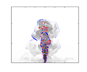
Note that, unlike the other two integrals, the integral momentum exchange (2.11) comprises two terms that affect the momentum from two different mechanisms – we separate this exchange as
 \begin{equation} \hat{m} = \hat{m}_V+\hat{m}_p, \end{equation}
where
 $$\begin{gather} \hat{m}_V = \frac{1}{\rm \pi} \oint_{\partial \varOmega} \frac{V_n w}{|\boldsymbol{N}_\perp|}\ {\rm d} \ell, \end{gather}$$
 $$\begin{gather}\hat{m}_p = \frac{1}{\rm \pi} \oint_{\partial \varOmega} \frac{-p N_z}{|\boldsymbol{N}_\perp|}\ {\rm d} \ell. \end{gather}$$
 The first term,  $\hat {m}_V$, is induced by the relative velocity transferring the momentum across the boundary. Consistent with the volume (2.10) and buoyancy (2.12), this represents the momentum entrainment when
  $V_n<0$, as opposed to detrainment when
  $V_n>0$. The additional term
  $\hat {m}_p$ is the momentum exchange induced by the pressure at the boundary. Noting the signs, (2.6) indicates that the pressure effect
  $\hat {m}_p$ tends to reduce the vertical momentum flux
  $\hat {M}$ within the flow.
Time-averaging the integral equations (2.5)–(2.7) yields the conditionally averaged plume equations
 $$\begin{gather} \frac{\,{\rm d} \langle \hat{Q} \rangle}{\,{\rm d} z} =-\langle \hat{q} \rangle, \end{gather}$$
 $$\begin{gather}\frac{\,{\rm d} \langle \hat{M} \rangle}{\,{\rm d} z} + \frac{\,{\rm d} \langle \hat{P} \rangle}{\,{\rm d} z} = \langle \hat B \rangle -\langle \hat{m}_V \rangle-\langle \hat{m}_p \rangle, \end{gather}$$
 $$\begin{gather}\frac{\,{\rm d} \langle \hat{F} \rangle}{\,{\rm d} z} =-\langle\, \hat{f} \rangle, \end{gather}$$
where  $\langle \cdot \rangle = ({1}/{T}) \int _{0}^{T} \cdot \, \,{\rm d} t$ is the time-averaging operator, with
  $T$ the averaging duration. These equations are identical in form to the classical plume equations of the boundary fluxes (van Reeuwijk & Craske Reference van Reeuwijk and Craske2015, e.g. before parametrisation), but note that no Reynolds averaging has been used, therefore
  $\langle \hat M \rangle$ and
  $\langle \hat F \rangle$ represent the total fluxes rather than the Reynolds-averaged mean fluxes.
2.3. Pointwise exchange rates
Following Yurtoglu et al. (Reference Yurtoglu, Carton and Storti2018), we convert the line integral to a surface integral, since surface integrals are simpler to evaluate computationally than line integrals. To do so, we first define an  $x$–
$x$– $y$ plane normal
  $\boldsymbol{n} n = \boldsymbol {\nabla }_\perp \chi /|\boldsymbol {\nabla }_\perp \chi |$ that again points into the domain of interest. For the line integral of an arbitrary scalar or vector component
  $X$, after using
  $\boldsymbol{n} \boldsymbol {\cdot } \boldsymbol{n} = 1$, the two-dimensional divergence theorem (taking into account the inward-pointing normal) and partial integration, we obtain
 \begin{equation} \oint_{\partial \varOmega} X\ {\rm d} \ell =\oint_{\partial \varOmega} X \boldsymbol{n} \boldsymbol{\cdot} \boldsymbol{n}\ {\rm d} \ell =- \int I\,\boldsymbol{\nabla}_\perp \boldsymbol{\cdot} (X \boldsymbol{n})\ {\rm d}\,A = \int X\,\boldsymbol{\nabla}_\perp I \boldsymbol{\cdot} \boldsymbol{n}\ {\rm d}\,A. \end{equation}
Here, the term  $\boldsymbol {\nabla }_\perp I \boldsymbol {\cdot } \boldsymbol{n}$ represents a delta distribution that samples the boundary
  $\partial \varOmega$.
When substituting  $X = 1$ into (2.18), the perimeter of the boundary
  $\partial \varOmega$ can be written as a surface integral
 \begin{equation} {\rm \pi}\hat{l} = \int e_l\ {\rm d}\,A, \quad e_l = \boldsymbol{\nabla}_\perp I \boldsymbol{\cdot} \boldsymbol{n}, \end{equation}
where  $e_l$ is the pointwise boundary length. The quantity
  $e_l(\boldsymbol{x},t)$ is local and instantaneous, and is zero everywhere except at the position of the interface,
  $\partial \varOmega$. Due to the presence of the delta distribution, the expression is singular in the theoretical limit, while its numerical approximation will be dependent on the spatial resolution – hence only spatial integrals can be examined meaningfully.
Similarly,  $\hat q$,
  $\hat m$ and
  $\hat f$ can be expressed in terms of surface integrals as
 $$\begin{gather} {\rm \pi}\hat{q} = \int e_q\ {\rm d}\,A, \quad {\rm \pi}\hat{m} = \int e_m\ {\rm d}\,A, \quad {\rm \pi}\hat{f} = \int e_f\ {\rm d}\,A, \end{gather}$$
 $$\begin{gather}e_q =\frac{V_n}{| \boldsymbol{N}_\perp|}\,e_l,\quad e_m =\underbrace{\frac{V_n w}{| \boldsymbol{N}_\perp|}\, e_l}_{e_{m,V}}+\underbrace{\frac{-pN_z}{| \boldsymbol{N}_\perp|} e_l}_{e_{m,p}}, \quad e_f =\frac{V_n b}{| \boldsymbol{N}_\perp|}\,e_l. \end{gather}$$
Here,  $e_q$ is the pointwise volume exchange rate (of dimension
  $\mathrm {T^{-1}}$),
  $e_m$ is the pointwise vertical-momentum exchange rate (of dimension
  $\mathrm {LT^{-2}}$), and
  $e_f$ is the pointwise buoyancy exchange rate (of dimension
  $\mathrm {LT^{-3}}$). Note that, consistent with
  $V_n(\boldsymbol{x},t)$, a negative value of
  $e_q(\boldsymbol{x},t)$ represents entrainment of volume flux into the domain of interest, and a positive value represents detrainment.
As the fountain is statistically axisymmetric, we introduce a Reynolds-averaging operator defined as (e.g. Craske & van Reeuwijk Reference Craske and van Reeuwijk2015; van Reeuwijk et al. Reference van Reeuwijk, Sallizoni, Hunt and Craske2016; Huang et al. Reference Huang, Burridge and van Reeuwijk2023)
 \begin{equation} \bar{X}(r,z) \equiv \frac{1}{2{\rm \pi} T} \int_{0}^{T}\int_{0}^{2{\rm \pi}} X(r,\theta,z,t) \, \,{\rm d} \theta\ {\rm d} t, \end{equation}
where  $X$ is an arbitrary field, and
  $\theta$ is the azimuthal direction. Time averaging of (2.19a,b) and (2.20a–c), and using the definition of the Reynolds average above, yields
 $$\begin{gather} \langle \hat{l} \rangle = 2 \int_0^\infty \bar{e}_l \,r\ {\rm d} r , \quad \langle \hat{q} \rangle= 2 \int_0^\infty \bar{e}_q r\ {\rm d} r , \end{gather}$$
 $$\begin{gather}\langle \hat{m} \rangle = 2 \int_0^\infty \bar{e}_m \, r\ {\rm d} r , \quad \langle\, \hat{f} \rangle = 2 \int_0^\infty \bar{e}_f \, r\ {\rm d} r , \end{gather}$$
which provides an explicit link between the time-averaged boundary integral (e.g.  $\langle \hat {q} \rangle$) and the integral of the Reynolds-averaged pointwise exchanges (e.g.
  $\bar {e}_q$) over the horizontal area. Since Reynolds averaging involves integration over the azimuthal direction, the quantities
  $\bar {e}$ are not resolution-dependent and have a clearly defined meaning: they represent the interface length or the net exchange across the interface at radius
  $r$, respectively. Radially integrating the Reynolds-averaged pointwise length
  ${\bar {e}}_l$ and net exchange
  $\bar {e}_q$,
  $\bar {e}_m$,
  $\bar {e}_f$ then provides the averaged integral length
  $\langle \hat {l} \rangle$ and net exchange
  $\langle \hat {q} \rangle$,
  $\langle \hat {m} \rangle$,
  $\langle \,\hat {f} \rangle$, respectively, on a particular horizontal plane.
2.4. Splitting entrainment and detrainment processes
Some parametrisations distinguish between entrainment and entrainment definitions, e.g. for turbulent fountains (Bloomfield & Kerr Reference Bloomfield and Kerr2000) or turbulent clouds (De Rooy & Siebesma Reference De Rooy and Siebesma2008). The current framework allows explicit calculation of these quantities. Using that  $e_q<0$,
  $e_q>0$ (whose sign is consistent with
  $V_n$) represent entrainment and detrainment, respectively, the pointwise exchange rates can be written as
 \begin{equation} e_X = e_X^++ e_X^-, \quad e_X^-= e_X\,H(-e_q), \quad e_X^+= e_X\,H(e_q), \end{equation}
where  $X$ is
  $l$,
$l$,  $q$,
$q$,  $m$ or
  $f$. With (2.19a,b) and (2.20a–c), this implies that the boundary integrals can be decomposed as
 \begin{equation} \hat{l} = \hat{l}^++ \hat{l}^-, \quad \hat{q} = \hat{q}^++ \hat{q}^-, \quad \hat{m} = \hat{m}^++ \hat{m}^-, \quad\hat{f} = \hat{f}^++ \hat{f}^- . \end{equation}
The momentum exchange term  $\hat m$ can be split into an entrainment term
  $\hat m_V = \int e_{m,V}\ {\rm d}\,A$ and a pressure term
  $\hat m_p = \int e_{m,p}\ {\rm d}\,A$, which each can be decomposed as
 \begin{equation} \hat{m}_V = \hat{m}_V^++ \hat{m}_V^-,\quad \hat{m}_p = \hat{m}_p^++ \hat{m}_p^- . \end{equation}
Note that the superscript represents only the integral over the area where fluid entrainment (indicated by ‘ $-$’) and detrainment (indicated by ‘
 $+$’) occur, but not the sign of the term itself. Due to the linearity of the time-averaging operator, (2.26a–b) also hold for the averaged quantities.
3. Case description and boundary specification
For the data analysis, use will be made of the highly resolved simulation of a turbulent forced fountain described in Huang et al. (Reference Huang, Burridge and van Reeuwijk2023). This is a high-Reynolds-number forced fountain (Burridge, Mistry & Hunt Reference Burridge, Mistry and Hunt2015; Hunt & Burridge Reference Hunt and Burridge2015) with source Reynolds number  $Re_0 = w_0r_0/\nu = 1667$ and source Froude number
  $Fr_0= w_0/\sqrt {|b_0|\,r_0}=21$, where
  $w_0>0$ is the uniform source vertical velocity,
  $r_0$ is the source radius,
  $b_0<0$ is the uniform source buoyancy, and
  $\nu$ is the fluid viscosity. The simulation domain has size
  $160r_0 \times 160r_0 \times 100 r_0$. The height is approximately twice the fountain height in the quasi-steady state to ensure that the domain top does not affect the fountain motion. Neumann boundary conditions for both velocity and buoyancy are applied at the domain top. At the domain bottom, a Neumann boundary condition is applied for buoyancy, and a free-slip boundary condition for velocity except for the source. Periodical boundary conditions are applied at four sides. In terms of the jet length
  $L_F= r_0Fr_0$ (Turner Reference Turner1966), which will be used to scale all lengths, the radius is
  $r_0 \approx 0.05L_F$. The simulation was performed with SPARKLE (Craske & van Reeuwijk Reference Craske and van Reeuwijk2015), a fully parallelized code for direct numerical simulation, which solves the incompressible Navier–Stokes equations under the Boussinesq approximation with fourth-order accuracy in space, and third-order accuracy in time. The domain is discretized with a uniform Cartesian grid of
  $1280^3$ cells. The simulation duration was
  $5400\,\text {s}$, which is equivalent to
  $24.5\, T_F$, where
  $T_F = \sqrt {r_0/|b_0|}\,Fr_0$ is the dominant time scale for forced fountains (Burridge & Hunt Reference Burridge and Hunt2013). Herein, we use these scales and fountain source momentum flux
  $M_0$ and buoyancy flux
  $F_0$ to normalise all quantities, making our findings applicable directly to all turbulent fountain flows with source Froude number
  $Fr_0 \gtrsim 4$ (Hunt & Burridge Reference Hunt and Burridge2015). For example, we use
  $q_F = L_F^2/T_F = M_0^{1/2}$,
  $m_F = M_0/L_F$ and
  $f_F = F_0/L_F$ to normalise all quantities concerning the entrainment of volume, momentum and buoyancy, respectively. For further simulation details, including a full validation of these simulations, see Huang et al. (Reference Huang, Burridge and van Reeuwijk2023).
As introduced, we focus on entrainment statistics across two instantaneous fountain boundaries – the outer boundary and the inner boundary. The instantaneous outer boundary (hereafter denoted by the subscript  $f$) is identified using the buoyancy, i.e.
  $\chi =|b|$ with
  $\chi _0=|b_c|$, where
  $|b|$ represents the absolute value of the buoyancy field. The threshold is set to
  $|b_c| = 3.6 \times 10^{-3}\,|b_0|$, consistent with the threshold in Huang et al. (Reference Huang, Burridge and van Reeuwijk2023), which is deduced from the buoyancy at the height of the cap base. Huang et al. (Reference Huang, Burridge and van Reeuwijk2023) reported that the outer boundary encloses almost all (negatively) buoyant fluid, and showed that reasonable variation of the threshold does not influence statistics significantly, including those concerning entrainment by the fountain.
The inner boundary (hereafter denoted by the subscript  $i$) is harder to define. It is intuitive to argue that
  $w>0$ is the natural criterion. Indeed, this is the default criterion to identify the upflow when analysing Reynolds-averaged quantities (Williamson, Armfield & Lin Reference Williamson, Armfield and Lin2011; Huang et al. Reference Huang, Burridge and van Reeuwijk2023). However, since the flow is turbulent, a threshold of zero would result in unwanted fluid being contained in the upflow; for example, slowly falling rotating turbulent fluid may contain regions of fluid that are, instantaneously, travelling upwards, i.e. patches of fluid with vertical velocity
  $w>0$ are contained within the turbulent downflow – we see evidence of this within our data. In addition, there are irrotational patches of fluid within the ambient for which
  $w>0$, which renders this criterion unhelpful. One could consider more complex composite criteria to solve this issue (for example, conditioning on both the velocity and buoyancy field simultaneously); however, this would require sophisticated and more computationally intensive algorithms that are beyond the scope of the current study.
Herein, we opt for a simpler, yet effective, solution by using  $\chi =w$ with a small positive threshold
  $\chi _0=0.07 w_0$. Selection of this threshold was based on a sensitivity study – there being no uniquely appropriate choice, mathematically. We tested thresholds in the range
  $0 \leq \chi _0 \leq 0.10 w_0$. As expected, lower thresholds within this range gave rise to the inclusion of unwanted fluid within the domain of interest; for example, fluid clearly within the downflow being included in the fountain upflow, and vice versa. Thresholds in the range
  $0.07 w_0 \leq \chi _0 \leq 0.09 w_0$ were deemed broadly suitable, with a threshold
  $0.07$ being selected as the smallest threshold that captures the most instantaneous upflow region but is broadly unaffected by the presence of unwanted fluid. For our data, this threshold is relatively small compared to the characteristic velocity over most heights of the fountain. In addition, as we demonstrate in § 4, our choice is not expected to have substantially affected the vertical profile of exchanges.
4. Results
4.1. Boundary statistics
Figure 2 shows a greyscale image of the forced fountain constructed in two halves; the left and right halves show snapshots of the instantaneous and Reynolds-averaged buoyancy fields, respectively. The greyscale map of the buoyancy field is normalised by  $|b_0|/Fr_0$. A thin white layer at the bottom over the horizontal region relatively far from the source, namely
  $|x/L_F|\geq 0.4$, can be observed, due to the manually set nudging area that avoids accumulation of buoyancy at the bottom boundary (Huang et al. Reference Huang, Burridge and van Reeuwijk2023). Overlaid on the right-hand side are the Reynolds-averaged inner boundary
  $r_i$, the outer boundary
  $r_f$, and the streamlines (see Huang et al. Reference Huang, Burridge and van Reeuwijk2023): the inner boundary
  $r_i$ is composed of the points of zero Reynolds-averaged vertical velocity, and the outer boundary
  $r_f$ is composed of the points where the Reynolds-averaged (absolute) buoyancy reduces to
  $|b_c|$, the same threshold as we define for the instantaneous boundary.

Figure 2. The forced fountain. Left half: a snapshot of the instantaneous buoyancy field together with the time-averaged characteristic inner and outer radii  $\langle \hat {r}_i \rangle$,
  $\langle \hat {r}_f \rangle$ (solid lines), and the location of
  $r_{50}$ of the fountain outer boundary and the upflow (dash-dotted lines), with the coloured band marking the interval between
  $r_{95}$ (left bound) and
  $r_{5}$ (right bound). Right half: Reynolds-averaged buoyancy field, together with interface positions of the inner and outer boundary
  $r_i$,
  $r_f$ inferred from Reynolds-averaged statistics, and the streamlines (black lines). The horizontal dashed lines on both sides present the location of the fountain cap base of the time-averaged conditional fountain and Reynolds-averaged fountain, respectively.
In order to develop an understanding of the location of the instantaneous interface, the radial locations associated with the areas within the inner and outer boundaries are determined according to
 \begin{equation} \langle \hat{r}_i \rangle ^2 = \langle \hat{A}_i \rangle , \quad \langle \hat{r}_f \rangle ^2 = \langle \hat{A}_f \rangle , \end{equation}
where  $\langle \hat {A}_i \rangle$ and
  $\langle \hat {A}_f \rangle$ are the time-averaged areas of the upflow and the whole fountain, respectively. These boundaries are marked by solid blue and orange lines on the left-hand side of figure 2, respectively. At the particular instant shown, the outer boundary of the fountain (as inferred from the instantaneous buoyancy field) can, for example, be seen to lie well within, and well outside the solid orange line marking
  $\langle \hat {r}_f \rangle$.
In order to quantify the variability of the instantaneous interface location, we selected three radial locations,  $r_5$,
  $r_{50}$ and
  $r_{95}$, for both the inner (blue) and outer (orange) boundaries, that correspond to 5 %, 50 % and 95 % of the contribution to
  $\langle{\hat {l}}\rangle$, specifically via
  $2 \int _0^{r_\alpha } \overline {e}_l\, r\, \,{\rm d} r=({\alpha }/{100}) \langle \hat {l} \rangle$, where
  $\alpha$ is a percentage. Note that near the fountain top, i.e.
  $z/L_F \gtrsim 1.9$ for the inner boundary and
  $z/L_F \gtrsim 2.3$ for the outer boundary, the vertical variation of
  $r_{\alpha }$ is not reliable as there are insufficient samples for accurate statistics. The band between
  $r_{95}$ and
  $r_{5}$ shows that the instantaneous boundaries of both the outer and inner boundaries exhibit broad fluctuations, with
  $r_{95}$ about twice as large as
  $r_{5}$ for both boundaries. Note that for
  $z/L_F \gtrsim 1$,
  $r_{95}$ is close to the Reynolds-averaged boundary (i.e.
  $r_i$ or
  $r_f$ in the right half of figure 2), and
  $r_{50}$ is very close to the time-averaged characteristic radius (i.e.
  $\langle \hat {r}_i \rangle$ or
  $\langle \hat {r}_f \rangle$).
The total height of the fountain, indicated by the time-averaged outer boundary  $\langle \hat {r}_f \rangle$, is
  $z/L_F \approx 2.40$, which is consistent with the Reynolds-averaged statistics on the right and the heights reported by the literature (for a review, see Hunt & Burridge Reference Hunt and Burridge2015). In the statistically steady state, the fluid in the region near the top experiences a number of large-scale fluctuations characterised by the formation and collapse of large-scale fluid structures, i.e. the direction of the fluid reverse near the top. We identify this near-top region as a ‘fountain cap’ to consider the fountain fluid that is influenced by the dynamics near the top. The fountain cap is defined above a height that is termed the fountain cap base. Consistent with Huang et al. (Reference Huang, Burridge and van Reeuwijk2023), we define the fountain cap base at a height where the averaged radius of upflow is the largest. Using this definition, the present conditional statistics yield a time-averaged cap base location
  $z/L_F = 1.58$, very close to the height
  $z/L_F = 1.62$ from the Reynolds-averaged statistics (Huang et al. Reference Huang, Burridge and van Reeuwijk2023). The two cap bases are labelled with horizontal dashed lines on both sides of figure 2. Indeed, different definitions of the fountain cap base have been proposed in the literature (Mcdougall Reference Mcdougall1981; Shrinivas & Hunt Reference Shrinivas and Hunt2014; Awin et al. Reference Awin, Armfield, Kirkpatrick, Williamson and Lin2018). However, Huang et al. (Reference Huang, Burridge and van Reeuwijk2023) have clarified that all these different definitions resulted in some very similar fountain cap bases to our fountain statistics. Hereafter, the cap base will be marked in the figures when necessary, as a reminder of the influence of the top.
4.2. Entrainment statistics
Figure 3 shows an instantaneous snapshot of the pointwise exchange rate  $e_q$ across the fountain outer boundary and inner boundary, at the three selected planes: one central vertical plane, and two different horizontal planes at
  $z/L_F = 1.62$ and
  $1.18$, which are approximately the fountain cap base and the fountain half-height, respectively.

Figure 3. Instantaneous pointwise volume exchange  $e_q$ across the inner and outer boundaries using a symmetric colour scale ranging from blue (entrainment) to red (detrainment). The darker colour represents the larger magnitude of the exchange. Plotted in the background is the instantaneous buoyancy field: (a) central vertical plane, (b) horizontal plane
  $z/L_F = 1.62$, (c) horizontal plane
  $z/L_F = 1.18$. The horizontal dashed line represents the height of the fountain cap base.
Here,  $e_q$ is displayed using a symmetric colour map that ranges from blue (
 $e_q<0$, entrainment) to red (
 $e_q>0$, detrainment); a colour bar is not shown since
  $e_q$ contains a delta distribution implying that its value depends on the grid size. As expected, figure 3 shows that there is only instantaneous entrainment at the outer boundary. Note that no results are shown below
  $z/L_F=0.66$; in this region, the downflow is affected by the bottom boundary (see the outer boundary and streamlines in figure 2), so that this region is excluded from all further analyses. At the inner boundary, entrainment (blue) and detrainment (red) co-exist instantaneously. Although the value of
  $e_q$ is not meaningful in itself, the relative magnitude is worthy of comparison. The magnitude of
  $e_q$ at the inner boundary is generally larger than that at the outer boundary, which is in accord with the stronger local turbulence at the inner boundary evident within our data (not shown), presumably due to the shearing interactions between the rising upflow and falling downflow. The colour also indicates the momentum and buoyancy exchanges. At the inner boundary the buoyancy is always negative and the vertical velocity is
  $0.07w_0$ due to the threshold, therefore in the blue area, these properties are entrained into the upflow, while in the red area they are detrained. However, the momentum exchange driven by the pressure still requires more specific statistics.
Figure 4 shows the time-averaged length fractions of the entrainment and detrainment to the total boundary perimeter, respectively. Here,  $\langle \hat {l}_i^- / \hat {l}_i \rangle$ and
  $\langle \hat {l}_i^+ / \hat {l}_i \rangle$ are the ratios of inner boundary, and
  $\langle \hat {l}_f^- / \hat {l}_f \rangle$ and
  $\langle \hat {l}_f^+ / \hat {l}_f \rangle$ are the ratios of the outer boundary. At the outer boundary, consistent with the observation in figure 3, most of the length of the boundary entrains, while only an insignificant ratio of the length detrains. At the inner boundary, reassuringly, both entrainment and detrainment occur. Near the source, the entrainment length is larger than the detrainment length. However, generally, the entrainment length decreases and the detrainment length increases with the height – at
  $z/L_F \approx 1.00$, half of the total boundary entrains and half detrains. Above that, the detrainment length is longer than the entrainment length. This indicates that near the source, the entrainment dominates the exchange, while near the top, the detrainment dominates.

Figure 4. The time-averaged length fraction of entrainment and detrainment to the total perimeter across (a) the outer boundary and (b) the inner boundary. The coloured band marks the first standard deviation interval of the time average. The ratio very near the top of the upflow, i.e.  $z/L_F \gtrsim 1.9$, and the fountain, i.e.
  $z/L_F \gtrsim 2.3$, is not shown due to the lack of sampled data. The horizontal dashed lines represent the heights of the fountain cap base.
Figure 5(a) shows the vertical variation of the time-averaged volume entrainment and detrainment at the outer boundary,  $\langle \hat {q}_f^- \rangle$,
  $\langle \hat {q}_f^+ \rangle$, respectively. The width of the correspondingly coloured shading highlights one standard deviation about the time-averaged mean. Also shown in the figure is the net volume exchange
  $q_f$ across the Reynolds-averaged boundaries
  $r_f$ (Huang et al. Reference Huang, Burridge and van Reeuwijk2023). Reassuringly, only entrainment is significant, with
  $\langle \hat {q}_f^- \rangle = \langle \hat {q}_f \rangle$. It can be seen that the Reynolds-averaged net entrainment
  $q_f$ is generally greater than the conditional time-averaged entrainment
  $\langle \hat {q}_f^- \rangle$, especially near the top (e.g.
  $z/L_F \gtrsim 2.0$). Clearly, this will provide a larger total entrainment flux when integrating from a reference height up to the fountain height. The reason is that the radial position of the time-averaged instantaneous interface
  $\langle \hat {r}_f \rangle$ is smaller than the Reynolds-averaged interface
  $r_f$, particularly near the top (see figure 2), which in turn implies a lower amount of entrained fluid. Reassuringly, if we use the position of
  $\langle \hat {r}_f \rangle$ as the interface to calculate the Reynolds-averaged entrainment flux
  $q_f$, then we find that it is close to
  $\langle \hat {q}_f^- \rangle$.

Figure 5. The time-averaged entrainment (with superscript −, yellow line (a–c) and green line in (d–f)), detrainment (with superscript +, brown line in (a–c) and blue line in (d–f)), and the net exchange (the sum of entrainment and detrainment, purple line in (d–f)) of (a,d) volume, (b,e) momentum and (c,f) buoyancy variation with the height. The panes (a–c) present those at the outer boundary, and the panels (d–f) present the inner boundary. The exchanges are compared with the net exchanges of the Reynolds-averaged fountain (black solid lines). The coloured band marks the first standard deviation interval of the time average. The dotted lines in (e) represent the time-averaged momentum exchange associated with the relative velocity  $\langle \hat {m}_V \rangle$ and its segregation. The difference between the dotted line and the solid line indicates the momentum exchange associated with the pressure, i.e.
  $\langle \hat {m}_{p,i} \rangle$ and its segregation.
Figures 5(b,c) show the momentum and buoyancy exchanges across the outer boundary, respectively. As expected, and consistent with the Reynolds average, there are insignificant time-averaged momentum and buoyancy exchanges across the outer boundary due to the very low magnitude of the momentum, pressure and buoyancy there. Figure 5(d) shows the volume exchanges at the inner boundary, and highlights that the net exchange  $\langle \hat {q}_i \rangle$ agrees closely with the Reynolds-average net exchange
  $q_i$ (as reported in Huang et al. Reference Huang, Burridge and van Reeuwijk2023). This provides confirmation that the methodology concerning the analysis of the instantaneous measurements, including the choice of velocity threshold, is appropriate. When
  $\langle \hat {q}_i \rangle$ is segregated into entrainment and detrainment events, it becomes apparent that at almost all heights,
  $\langle \hat {q}_i \rangle$ is small compared with either the entrainment fluxes
  $\langle \hat {q}_i^- \rangle$ or the detrainment fluxes
  $\langle \hat {q}_i^+ \rangle$ – evidence that entrainment and detrainment co-exist at the inner boundary, and that, typically, the two fluxes are comparable. The net volume exchange
  $\langle \hat {q}_i \rangle$ intersects zero at
  $z/L_F \approx 1.0$, close to its Reynolds-averaged counterpart. Note that this is also very close to the location where entrainment and detrainment have an equal length in figure 4(b). The time-averaged instantaneous entrainment peaks at
  $\langle \hat {q}_i^- \rangle \approx -0.39 q_F$ (at
  $z/L_F \approx 0.82$), and the detrainment peaks at
  $\langle \hat {q}_i^+ \rangle \approx 0.43 q_F$ (at
  $z/L_F \approx 1.31$).
Figure 5(e) shows the time-averaged momentum exchange  $\langle \hat {m}_{i} \rangle$ at the inner boundary, including the decomposed contributions of entrainment,
  $\langle \hat {m}_{i}^- \rangle$, and detrainment,
  $\langle \hat {m}_{i}^+ \rangle$. For
  $z/L_F \gtrsim 0.45$,
  $\langle \hat {m}_{i} \rangle$ is positive, indicating that the momentum exchange at the inner boundary decreases the upward vertical momentum flux within the upflow over most of the fountain height. This is broadly consistent with the Reynolds-averaged quantity
  $m_i$ at the inner boundary (Huang et al. Reference Huang, Burridge and van Reeuwijk2023; black line). Figure 5( f) shows the negative buoyancy exchanges at the inner boundary, with the horizontal axis normalised by
  $f_F$ (which is negative); therefore, the direction of exchange is aligned with that of the volume exchange. The quantity
  $\langle \,\widehat{f_i}^- \rangle$ represents the negative buoyancy entrained into the upflow, while
  $\langle \,\widehat{f_i}^+ \rangle$ represents the negative buoyancy detrained out of the upflow. The net
  $\langle \,\widehat{f_i} \rangle$ generally agrees well with the Reynolds average
  $f_i$ with the zero point at
  $z/L_F \approx 0.90$, slightly lower than that of
  $\langle q_i \rangle$. The buoyancy entrainment peaks at
 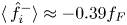 $\langle \,\hat {f}_i^- \rangle \approx -0.39 f_F$ (at
  $z/L_F \approx 0.82$), and the detrainment peaks at
  $\langle \,\hat {f}_i^+ \rangle \approx 0.43 f_F$ (at
  $z/L_F \approx 1.31$).
The net momentum exchange  $\langle \hat {m}_{i} \rangle$ is comprised of two contributions: one due to entrainment
  $\langle \hat {m}_{V,i} \rangle$, and one due to pressure
  $\langle \hat {m}_{p,i} \rangle$ (§ 2). These quantities are examined in figure 6(a), and shown, for comparison, alongside the Reynolds-averaged net momentum exchange
  $m_i$ (Huang et al. Reference Huang, Burridge and van Reeuwijk2023), and the integral buoyancy of the upflow
  $\langle \hat {B}_u \rangle$, the latter being a term on the right-hand-side of momentum equation (2.16). The figure shows that the exchange types are equal in magnitude and comparable to the integral buoyancy, so no terms are negligible a priori. The quantity
  $\langle \hat {m}_{V,i} \rangle$ is trivially related to
  $\langle \hat {q}_{i} \rangle$ since substitution of the constant threshold value
  $0.07 w_0$ (which identifies the inner boundary) into (2.14), and exploiting (2.10), yields directly
  $\langle \hat {m}_{V,i} \rangle =0.07 w_0 \langle \hat {q}_{i} \rangle$. This fact is borne out by our data (cf. the shape of
  $\langle \hat {m}_{V,i} \rangle$ marked by the dotted lines in figure 5(e), and that of
  $\langle \hat {q}_{i} \rangle$ in figure 5d).

Figure 6. (a) The time-averaged net momentum exchange  $\langle \hat {m}_{i} \rangle$ and its components net
  $\langle \hat {m}_{V,i} \rangle$ and net
  $\langle \hat {m}_{p,i} \rangle$, overlaid with the integral negative buoyancy of the upflow
  $\langle \hat {B}_u \rangle$, and the Reynolds-averaged momentum exchange
  $m_i$. (b) The pressure effect of net momentum exchange
  $\langle \hat {m}_{p,i} \rangle$ conditioned to the entrainment
  $\langle \hat {m}_{p,i}^- \rangle$ and detrainment
  $\langle \hat {m}_{p,i}^+ \rangle$ components.
Note that the difference between the dotted lines and solid lines in figure 5(e) indicates the pressure-induced momentum exchange (e.g.  $\langle \hat {m}_{p,i}^- \rangle$ and
  $\langle \hat {m}_{p,i}^- \rangle$). These data demonstrate that conditional momentum entrainment or detrainment is caused primarily by the decomposed components associated with entrainment or detrainment velocities. However, there is no intrinsic physical relevance to the term
  $\langle \hat {m}_{V,i} \rangle$, because of the need to impose a non-zero vertical velocity threshold (in our case,
  $0.07 w_0$) to avoid unexpected fluid in the upflow (see § 3). In theory, a zero vertical velocity threshold value is a natural choice for the inner boundary, which would result in the term
  $\langle \hat {m}_{V,i} \rangle$ being zero, leaving only the pressure exchange term
  $\langle \hat {m}_{p,i} \rangle$ of the dynamically active terms within the momentum exchange. Figure 6(a) compares the net momentum exchange across the inner boundaries when conditionally averaged,
  $\langle \hat {m}_{p,i} \rangle$, with that for the Reynolds-averaged net momentum exchange
  $m_i$, which in the case of Reynolds averaging is indeed to set the loci of zero vertical velocity (Huang et al. Reference Huang, Burridge and van Reeuwijk2023). The conditionally averaged
  $\langle \hat {m}_{p,i} \rangle$ term agrees well with the Reynolds-averaged momentum exchange
  $m_i$ below
  $z/L_F \approx 0.8$, and marginally lower than
  $m_i$ above that.
Figure 6(b) shows the pressure exchange term decomposed in its entrainment and detrainment terms. As can be seen, both  $\langle \hat {m}_{p,i}^- \rangle$ and
  $\langle \hat {m}_{p,i}^+ \rangle$ are positive. Recall that the conditioning is based on the local value of
  $V_n$ (§ 2) and the pressure has a negative sign in momentum equation (2.16), the fact that both are positive implies that pressure acts to remove momentum from the upflow both during entrainment and detrainment events. From the observation that
  $\langle \hat {m}_{p,i}^- \rangle$ is slightly larger than
  $\langle \hat {m}_{p,i}^+ \rangle$, we can conclude that the pressure effect is slightly larger during entrainment events.
Figure 7 shows the time-averaged ratio of the integrals, which represents the local entrainment/detrainment velocity  $\hat {q} / \hat {l}$, the locally exchanged vertical velocity
  $\hat {m} / \hat {q}$, and the locally exchanged buoyancy
  $\hat {f} / \hat {q}$, respectively. Note that the exchanged vertical velocity (momentum) and buoyancy across the outer boundary are not presented since these are insignificant. Figure 7(a) shows the local entrainment/detrainment velocities. As in earlier figures, the thick lines represent the mean value, and the shaded bands represent the range from the first standard deviation interval of the time average. The entrainment velocity at the outer boundary
  $\langle \hat {q}_f^- / \hat {l}_f^- \rangle$ is approximately constant over the entire fountain height and has very little fluctuation with time. Note that here, the absolute value is presented to show the magnitude of the velocity. At the inner boundary, beyond the near-source region, the entrainment velocity
  $\langle \hat {q}_i^- / \hat {l}_i^- \rangle$ and detrainment velocity
  $\langle \hat {q}_i^+ / \hat {l}_i^+ \rangle$ both decrease approximately linearly with height. Both are large compared with the entrainment velocity at the outer boundary. Combined with figure 4(b), we find that below
  $z/L_F \approx 1.0$, both the entrainment length and entrainment velocity are greater than those of detrainment, while above that, they are the opposite.

Figure 7. (a) Time-averaged absolute entrainment and detrainment velocity normalised with the fountain source vertical velocity  $w_0$. (b) Exchanged vertical velocity
  $w_i$ normalised by
  $w_0$. (c) Exchanged buoyancy
  $b_i$ at the inner boundary normalised by the absolute source buoyancy
  $|b_0|$.
Data for the averaged exchanged velocity  $\langle \hat {m}_{i}/\hat {q}_i \rangle /w_0$ are shown in figure 7(b), and indicate that over most of the fountain height, i.e.
  $z/L_F \gtrsim 0.45$, the exchanged velocity is approximately
  $0.05$ for entrainment and
  $0.08$ for detrainment. Note that these averaged quantities would both be the constant
  $0.07$ were it not for the contribution due to pressure within the momentum exchange. Figure 7(c) examines the time-averaged entrained and detrained buoyancy over the inner boundary
  $\langle \,\hat {f}_f^- / \hat {q}_f^- \rangle$ and
  $\langle \,\hat {f}_f^+ / \hat {q}_f^+ \rangle$, respectively. The values are normalised by the absolute source value
  $|b_0|$ to keep the negative sign of the buoyancy. We note that over the main interval of the upflow,
  $0.5 \leq z/L_F \leq 2.0$, the time-averaged entrained buoyancy is approximately
  $-0.33\,|b_0|$ while the detrained buoyancy is
  $-0.37\,|b_0|$, i.e. the averaged detrained buoyancy is always more negative than the averaged entrained buoyancy. This is because the detrainment transfers the upflow buoyancy outwards, while the entrainment transfers the downflow buoyancy into the upflow. The downflow buoyancy is inherently less negative than the upflow.
4.3. Entrainment coefficients
The entrainment model of Morton, Taylor & Turner (Reference Morton, Taylor and Turner1956) (hereinafter MTT) related the entrainment velocity across the plume edge to local characteristic scales via a constant entrainment coefficient, to characterise the bulk entrainment of a plume. Bloomfield & Kerr (Reference Bloomfield and Kerr2000) (hereinafter BK00) developed a bulk-averaged fountain model applying the entrainment coefficients to estimate the entrainment within the fountain. They separated the fountain into an upflow and a downflow, where the upflow is assumed to entrain from and detrain into the downflow, and the downflow entrains from and detrains into the upflow, and entrains from the environment. In this subsection, we recalculate the entrainment coefficients of the model of BK00 using conditional statistics, and compare them with measurements.
The BK00 parametrisation for the downflow entrainment flux across the outer boundary is given by
 \begin{equation} \langle \hat{q}_{f}^- \rangle = 2 r_{d} \omega_f, \end{equation}
with  $r_d$ the characteristic radius of the downflow, and
  $\omega _f$ the entrainment velocity given by
 \begin{equation} \omega_f =-\gamma\,|w_{d}|, \end{equation}
where  $|w_d|$ is the absolute value of the characteristic downflow velocity,
  $\gamma$ is the entrainment coefficient at the outer boundary, and the negative sign represents the entrainment velocity pointing into the flow in our framework.
At the inner boundary, BK00 assume that the upflow entrains from, and detrains into, the downflow with velocities  $\omega _i$ and
  $\omega _d$, respectively, producing an entrainment and detrainment flux given by
 \begin{equation} \langle \hat{q}_{i}^- \rangle = 2 r_{u} \omega_i, \quad \langle \hat{q}_{i}^+ \rangle = 2 r_{u} \omega_d, \end{equation}
where  $r_u$ is the characteristic radius of the upflow. BK00 parametrised the detrainment velocity as
 \begin{equation} \omega_d = \beta\,|w_{d}|, \end{equation}
where  $\beta$ is the detrainment coefficient. For the entrainment velocity
  $\omega _i$, BK00 proposed two possible parametrisations:
 \begin{equation} \omega_i^I =-\alpha^I (w_{u}+|w_{d}|) , \quad \omega_i^{II} =-\alpha^{II} w_{u}, \end{equation}
with associated entrainment coefficients  $\alpha ^I$ and
  $\alpha ^{II}$, respectively. The first parametrisation assumed that the entrainment velocity should be proportional to the difference in velocity between the upflow and downflow, while the second assumed that the entrainment velocity depends solely on the velocity within the upflow. Here, the characteristic values are associated with the vertical fluxes of the upflow (subscript
  $u$) and downflow (subscript
  $d$) (Bloomfield & Kerr Reference Bloomfield and Kerr2000; Huang et al. Reference Huang, Burridge and van Reeuwijk2023), given by
 \begin{equation} w_{u} \equiv \frac{\langle \hat{M}_u \rangle}{\langle \hat{Q}_u \rangle}, \quad r_{u} \equiv \frac{\langle \hat{Q}_u \rangle}{\langle \hat{M}_u \rangle^{1/2}}, \quad w_{d} \equiv \frac{\langle \hat{M}_d \rangle}{\langle \hat{Q}_d \rangle}, \quad r_{d} \equiv \sqrt{\frac{\langle \hat{Q}_u \rangle^2}{\langle \hat{M}_u \rangle}+ \frac{\langle \hat{Q}_d \rangle^2}{\langle \hat{M}_d \rangle}} . \end{equation}
 BK00 assumed that the downflow entrains similarly to a line plume, therefore taking  $\gamma _{00} = \beta _{00} = 0.147$ according to the entrainment coefficient of the line plume, where the subscript
  $00$ represents BK00. They assumed the upflow entrainment coefficient
  $\alpha ^{I}_{00} =\alpha ^{II}_{00} = 0.085$, which is the average of the jet value and plume value. With these coefficients, combining the exchange equations with the governing equations, the fountain model, which is a closed set of equations, can be solved. The result presented in BK00 was tuned to agree with the experimental data for the statistics of the steady mean fountain height. A sensitivity examination revealed that the predicted fountain height depends strongly on the choice of
  $\gamma _{00}$, but is almost not affected by
  $\beta _{00}$.
Figure 8 presents  $\alpha$,
  $\beta$ and
  $\gamma$ calculated using (4.2)–(4.7a–d). Figure 8(a) shows that the coefficient
  $\gamma$ is marginally greater than
  $\gamma _{00}$ but generally smaller than
  $0.20$, which supports the BK00 assumption that the downflow at the outer boundary is likely to entrain as a line plume. Figure 8(b) shows that near the source, below
  $z/L_F \approx 0.6$, the upflow entrainment coefficients
  $\alpha ^{I}$ and
  $\alpha ^{II}$ increase from below
  $0.085$ to over
  $0.147$. Above that, the two coefficients become approximately constant with the height:
  $\alpha ^{I} \approx 0.16$ and
  $\alpha ^{II} \approx 0.21$, respectively. The coefficient
  $\alpha ^I$ is more constant with height than
  $\alpha ^{II}$, which suggests that the parametrisation I, which accounts for the total shear between the upflow and downflow, is the better parametrisation.

Figure 8. The entrainment and detrainment coefficients at (a,b) the inner boundary and (c) the outer boundary, overlaid with vertical dashed lines showing the entrainment coefficients used in BK00,  $0.085$ and
  $0.147$. All the coefficients are shown up to the fountain cap base
  $z/L_F = 1.62$.
Figure 8(c) shows that the detrainment coefficient of the upflow is  $\beta \approx 0.80$ beyond the near source field, which is much larger than
  $\beta _{00}$. This is because in our data, the detrainment flux is comparable with the entrainment flux (as shown in figure 5d), but the characteristic downflow velocities
  $w_{d}$ are small compared with the characteristic upflow velocities
  $w_{u}$, resulting in the large detrainment coefficients determined herein. However, as mentioned before, BK00 showed that
  $\beta$ does not have a significant effect on predicting the fountain height.
As the BK00 model is a bulk model, the momentum and buoyancy exchange across the inner boundary is modelled as the product of the volume exchange and the characteristic velocity and buoyancy, where the characteristic values are, in effect, assumed to be those transported, i.e.
 $$\begin{gather} \langle \hat{m}_{i}^- \rangle = \langle \hat{q}_{i}^- \rangle w_d, \quad \langle\, \hat{f}_{i}^- \rangle = \langle \hat{q}_{i}^- \rangle b_d, \end{gather}$$
 $$\begin{gather}\langle \hat{m}_{i}^+ \rangle = \langle \hat{q}_{i}^+ \rangle w_u, \quad \langle\, \hat{f}_{i}^+ \rangle = \langle \hat{q}_{i}^+ \rangle b_u. \end{gather}$$
Equations (4.8a,b) model the momentum and buoyancy entrained into the upflow, respectively, and (4.9a,b) model those entrained into the downflow. Note that BK00 did not attempt to model the pressure effect on the momentum exchange. Consistent with (4.7a–d), the characteristic buoyancy is defined as
 \begin{equation} b_{u} \equiv \frac{\langle \hat{B}_u \rangle \langle \hat{M}_u \rangle}{\langle \hat{Q}_u \rangle^2}, \quad b_{d} \equiv \frac{\langle \hat{B}_d \rangle \langle \hat{M}_d \rangle}{\langle \hat{Q}_d \rangle^2}. \end{equation}
 Figure 9 compares the observed volume exchange and buoyancy exchange with the predictions of the entrainment parametrisations using the parameter values  $\alpha ^{I} = 0.16$,
  $\beta = 0.80$ and
  $\gamma = 0.19$. (We choose
  $\alpha ^{I}$ and its corresponding parametrisation simply due to the coefficient
  $\alpha ^I$ being more constant with height than
  $\alpha ^{II}$ over most fountain heights. However, we believe that
  $\alpha ^{II}$ and parametrisation II will not make substantial difference.) Here, the subscript
  $M$ denotes the predicted fluxes. Note that the predictions for the quantities of the upflow start above
  $z/L_F =0.66$ since the model requires characteristic values of the downflow in order to calculate predictions of the upflow – we attain reliable data for the downflow only above
  $z/L_F =0.66$. Figures 9(a,b) show that the predicted volume exchanges are in agreement with the simulation for both boundaries, which shows that the revised coefficients capture the volume entrainment and detrainment of the fountain well. Figure 9(c) shows that the model tends to underpredict the negative buoyancy entrained into the upflow, and overpredict the negative buoyancy detrained out of the upflow. This is because the characteristic buoyancy cannot represent the local transport buoyancy at the boundary appropriately – considering the distance from the centreline, the characteristic buoyancy of the upflow,
  $b_u$, is more negative than the local boundary value, which is, further, more negative than the characteristic buoyancy of the downflow,
  $b_d$. The net exchange of negative buoyancy tends to be overpredicted by the model.

Figure 9. The modelled exchanges compared with the simulation exchanges for: (a) volume flux across the outer boundary; (b) volume flux across the inner boundary; and (c) buoyancy exchange across the inner boundary. The data presented here are for  $0.66 \leq z/L_F \leq 1.62$, and the parameter values used are
  $\alpha ^{I} = 0.16$,
  $\beta = 0.80$ and
  $\gamma = 0.19$. The diagonal dashed lines represent perfect agreement.
The prediction of the momentum exchanges is more challenging, as mentioned before and argued in the following discussion. First, a substantial part of the momentum exchange at the inner boundary is determined by  $m_{V,i}$. Since the inner boundary was defined using a threshold
  $0.07 w_0$,
  $m_{V,i}$ is given simply by
  $0.07w_0 \langle \hat {q}_i \rangle$. This relation is shown in figure 10(a), and reassuringly shows excellent agreement between the parametrisation and the simulation data. However, this threshold was chosen by trial and error, and did not emerge from any fundamental insight or theoretical considerations; naturally, as mentioned, one would – for the momentum exchange only – desire to select a zero velocity threshold, in which case only the pressure term
  $\langle \hat {m}_{p,i} \rangle$ would contribute to the momentum exchange. Therefore, the net momentum exchange predicted by BK00, (4.8a,b), is compared with the pressure term
  $\langle \hat {m}_{p,i} \rangle$ in figure 10(b). Although we are aware that these two plotted quantities are induced by different mechanisms (note that the modelled term
  $\langle \hat {m}_{i} \rangle _M$ is associated with the entrainment velocity), their comparison is still worthy since they both represent the momentum exchange across the inner boundary. The figure shows that the parametrisation grossly overpredicts the simulation data. However, we note that this does not mean that
  $\langle \hat {m}_{p,i} \rangle$ is negligible – figure 6 shows that this quantity is of magnitude similar to the buoyancy term
  $\langle \hat {B} \rangle$. Our results therefore suggest that the BK00 parametrisation is not appropriate for predicting the momentum exchange.

Figure 10. (a) The product of the volume exchange  $\langle \hat {q}_{i} \rangle$ (including the conditional components) and the constant threshold
  $0.07w_0$ compared with the measured momentum exchange
  $\langle \hat {m}_{V,i} \rangle$. (b) The modelled net momentum exchange compared with the measured net momentum exchange
  $\langle \hat {m}_{p,i} \rangle$. The diagonal dashed lines represent perfect agreement.
4.4. Normalised entrainment density
By rearranging (2.23a,b) to be  $\int _0^\infty 2\bar {e}_l r/\langle \hat {l} \rangle\ {\rm d} r = 1$, the quantities
  $2\bar {e}_l r / \langle \hat {l} \rangle$ evidence how
  $\langle \hat {l} \rangle$ is distributed over the radial direction
  $r$, i.e.
  $2\bar {e}_l r / \langle \hat {l} \rangle$ represents a normalised exchange length density. Figure 11 shows the radial profiles of the normalised exchange length density at the two boundaries conditioned by entrainment and detrainment events, for both the inner and outer boundaries. Data are shown at the two vertical planes depicted in figure 3, i.e.
  $z/L_F = 1.18$ and
  $1.62$; vertical dash-dotted lines mark the local time-averaged characteristic radii
  $\langle \hat {r}_f \rangle$ and
  $\langle \hat {r}_i \rangle$. Figures 11(a,b) show the normalised exchange length associated with the outer boundary
  $2\bar {e}_{l,f} r / \langle \hat {l}_f \rangle$ at both heights. Here, the first subscript (
 $l$) represents the exchange length, and the second subscript (
 $\,f$) indicates that it is associated with the outer boundary; similarly hereinafter. Consistent with figure 4(a), there is mainly entrainment occurring at the fountain outer boundary, thus
  $\bar {e}_{l,f} \approx \bar {e}_{l,f}^-$ and
  $\langle \hat {l}_f \rangle \approx \langle \hat {l}_{f}^- \rangle$. The location of the time-averaged characteristic radius
  $\langle \hat {r}_f \rangle$ is close to the location of the maximum value of
  $2\bar {e}_{l,f} r / | \langle \hat {l}_{f} \rangle |$ at both heights. The profiles can be approximated well by a Gaussian profile (black dashed line)
 \begin{equation} \frac{2 \bar{e}r}{|\langle \hat{l} \rangle|} \approx \text{sgn} (\langle \hat{l} \rangle)\frac{1}{\sqrt{2 {\rm \pi}}\,\sigma_g}\exp\left(-\frac{(r-r_g)^2}{2 \sigma_g^2} \right), \end{equation}
of which the distribution parameters  $r_g/\langle \hat {r}_f \rangle$ and
  $\sigma _g/\langle \hat {r}_f \rangle$ are listed within the figure. Note that
  $\langle \hat {r}_f \rangle /L_F = 0.60, 0.69$ at
  $z/L_F = 1.62, 1.18$, respectively.

Figure 11. Normalised exchange length density  $2\bar {e}_{l,f}r / |\langle \hat {l}_f \rangle |$ as a function of
  $r$ associated with the outer boundary, plotted at (a)
  $z/L_F = 1.62$ and (b)
  $z/L_F= 1.18$. Normalised exchange length density
  $2\bar {e}_{l,i}r / |\langle \hat {l}_i \rangle |$ associated with the inner boundary at (c)
  $z/L_F = 1.62$ and (d)
  $z/L_F= 1.18$. Vertical dash-dotted lines mark the local time-averaged characteristic radius of the outer boundary
  $\langle \hat {r}_f \rangle$ and inner boundary
  $\langle \hat {r}_i \rangle$, correspondingly. Gaussian profiles fitted to the data are marked as dashed curves, whose distribution parameters are listed in the figure in the corresponding colour.
Figures 11(c,d) show the normalised exchange length associated with the inner boundary at both heights. Like the outer boundary, the normalised exchange length density  $2\bar {e}_{l,i} r / \langle \hat {l}_i \rangle$ at the inner boundary is also well fitted by a Gaussian profile. The exchange length density peaks near the location of the time-averaged characteristic radius
  $\langle \hat {r}_i \rangle$ at both heights. When segregating to the conditional exchange length densities, the entrainment length density
  $2\bar {e}_{l,i}^-r / |\langle \hat {l}_i \rangle |$ and the detrainment length density
  $2\bar {e}_{l,i}^+r / |\langle \hat {l}_i \rangle |$ are also both well approximated by Gaussian profiles, i.e. the entire exchange perimeter, which is Gaussian-like, results from the superposition of two Gaussian-like profiles each associated with entrainment or detrainment. Note that the normalisation uses the total length
  $|\langle \hat {l}_i \rangle |$ to compare directly the entrainment and detrainment densities, implying that (4.11) needs to be multiplied by an enhancement
  $|\langle \hat {l}_i^- \rangle |/|\langle \hat {l}_i \rangle |$ or
  $|\langle \hat {l}_i^+ \rangle |/|\langle \hat {l}_i \rangle |$ for the entrainment and detrainment expressions, respectively. Again, the distribution parameters for the Gaussian profile, here normalised by the averaged radius of the inner boundary,
  $r_g/\langle \hat {r}_i \rangle$ and
  $\sigma _g/\langle \hat {r}_i \rangle$, are listed in the figure. We find the radius
  $\langle \hat {r}_i \rangle /L_F = 0.19, 0.17$ at
  $z/L_F = 1.62, 1.18$, respectively. The parameters confirm that the total and conditional profiles have practically identical
  $r_g$ and
  $\sigma _g$, so they can remain in the Gaussian profile while in the superposition.
Analogous to the length, rearranging (2.23a,b) and (2.24a,b) in terms of  $q,m$ and
  $f$, respectively, we obtain the normalised exchange density of volume
  $2\bar {e}_q r / |\langle \hat {q} \rangle |$, momentum
  $2\bar {e}_m r / |\langle \hat {m} \rangle |$, and buoyancy
  $2\bar {e}_f r / |\langle \,\hat {f} \rangle |$, respectively, presented in figure 12. Figures 12(a,b) show the volume exchange density associated with the outer boundary
  $2\bar {e}_{q,f} r / | \langle \hat {q}_f \rangle |$ at both heights. The absolute value of
  $\langle \hat {q}_f \rangle$ is used in order to keep the signs of the exchange density consistent with the rest of the paper: negative represents entrainment, while positive represents detrainment, as labelled in the figure. Consistent with figure 5(d), there is only volume entrainment at the fountain boundary, thus
  $\bar {e}_{q,f} \approx \bar {e}_{q,f}^-$. Again, the profiles can be approximated well by a Gaussian profile with the distribution parameters
  $r_g/\langle \hat {r}_f \rangle$ and
  $\sigma _g/\langle \hat {r}_f \rangle$. The location of the time-averaged characteristic radius
  $\langle \hat {r}_f \rangle$ is close to the location of the maximum value of
  $2\bar {e}_{q,f} r / | \langle \hat {q}_{q,f} \rangle |$ at both heights, as reassured by the ratio
  $r_g/\langle \hat {r}_f \rangle$ being unity. As figure 5(e, f) have shown, the momentum and buoyancy exchanges at the outer boundary are insignificant, therefore the momentum exchange density and buoyancy exchange density at the outer boundary are not presented here.

Figure 12. Normalised volume exchange density  $2\bar {e}_{q,f}r / |\langle \hat {q}_f \rangle |$ as a function of
  $r$ associated with the outer boundary, plotted at (a)
  $z/L_F = 1.62$ and (b)
  $z/L_F= 1.18$. Normalised (c, f) volume exchange density
  $2\bar {e}_{q,i}r / |\langle \hat {q}_i \rangle |$, (d,g) momentum exchange density
  $2\bar {e}_{m,i}r / |\langle \hat {m}_i \rangle |$ and (e,h) buoyancy exchange density
  $2\bar {e}_{f,i}r / |\langle \,\hat {f}_i \rangle |$ associated with the inner boundary, at (c–e)
  $z/L_F = 1.62$ and ( f–h)
  $z/L_F= 1.18$. Vertical dash-dotted lines mark the local time-averaged characteristic radius of the outer boundary
  $\langle \hat {r}_f \rangle$ and inner boundary
  $\langle \hat {r}_i \rangle$, correspondingly. Gaussian profiles fitted to the data are marked as dashed curves. As labelled in (a), the area above the horizontal axis belongs to detrainment, while that below belongs to entrainment for all the exchanges.
Figures 12(c–h) show the radial variation of volume exchange density, momentum exchange density and buoyancy exchange density associated with the inner boundary, respectively, at both heights. Here again, due to the normalisation, each profile has been multiplied by a corresponding enhancement, e.g.  $|\langle \hat {q}_i^- \rangle |/|\langle \hat {q}_i \rangle |$. It is striking that all the conditional entrainment and detrainment densities of volume, momentum and buoyancy (coloured lines), at both heights, are well approximated by the Gaussian profiles (distribution parameters
  $r_g/\langle \hat {r}_f \rangle$ and
  $\sigma _g/\langle \hat {r}_f \rangle$ are marked within the figure). However, all the net normalised exchange densities, which are the superposition of the entrainment and detrainment events, are clearly non-Gaussian-like (solid black lines). The net profile shape depends strongly on
  $z$ – for
  $z/L_f = 1.18$ (figures 12 f,h), there is remarkable entrainment of volume and buoyancy for
  $r \lesssim \langle \hat {r}_i \rangle$ and detrainment further away from the fountain centreline. However, at the higher level,
  $z/L_f = 1.62$ (figures 12c,e), insignificant net entrainment of volume and buoyancy is observed. Since, for each case, the distribution parameters
  $\sigma _g/\langle \hat {r} \rangle$ in the conditional entrainment and detrainment profiles are approximately identical, the non-Gaussian-like profile of net exchange is due to the distribution parameters
  $r_g/\langle \hat {r}_i \rangle$ in the two conditional profiles being different (i.e. the difference is generally greater than
  $0.10$). Here, the fact that for all the exchanges, the entrainment and detrainment exchange densities have a larger amplitude than the net exchange density confirms once more that the conditional entrainment and detrainment terms are large compared with the net (consistent with figures 5d–f).
The second feature noted for all kinds of exchanges, i.e. of volume, momentum and buoyancy, is that  $r_g/\langle \hat {r}_i \rangle$ of conditional profiles at both heights are all close to
  $1$, with
  $r_g/\langle \hat {r}_i \rangle$ of the entrainment profile always smaller than that of the detrainment. This shows that the maximum value of the entrainment (and detrainment) density is close to the location of the time-averaged characteristic radius
  $\langle \hat {r}_i \rangle$. However, the conditional entrainment density peaks closer to the fountain centreline than the detrainment, which explains the propensity for net entrainment closer to the fountain centreline, and detrainment further away. This is possible due to the anisotropy and inhomogeneity of the turbulence within the fountain, which are worthy of further study.
Moreover, we note that figures 12(d,g) show the normalised momentum exchange densities at the inner boundary  $2\bar {e}_{m,i} r / |\langle \hat {m}_i \rangle |$, including the entrainment and detrainment events. As illustrated before, the momentum exchange should be consistent with the volume exchange if only
  $\langle \hat {m}_V \rangle$ was considered. Hence the difference between the profiles of volume (figures 12c, f) and momentum (figures 12d,g) is driven by the pressure effect. The pressure does not affect entrainment and detrainment significantly on the Gaussian fit. However, the parameter
  $r_g/\langle \hat {r}_i \rangle$ indicates that the pressure makes the peaks of conditional momentum densities, especially the entrainment density, occur closer to the centreline compared with the volume. Additionally, the pressure also affects the amplitude enhancement significantly.
Recall that the net normalised exchange length densities (figure 11) are approximately Gaussian-like, while net normalised exchange densities of volume, momentum and buoyancy are not (figure 12), due to the relatively large difference between the distribution parameters  $r_g/\langle \hat {r} \rangle$ of entrainment and detrainment events. This is suspected to be influenced by the averaged exchange velocity, momentum and buoyancy across the boundary that separates
  $r_g/\langle \hat {r} \rangle$ of entrainment and detrainment further. Therefore, figure 13 shows the radial distribution of the averaged entrainment velocity
  $\bar {e}_{q} / \bar {e}_{l}$, averaged exchanged vertical velocity
  $\bar {e}_{m} / \bar {e}_{q}$ and averaged exchanged buoyancy
  $\bar {e}_{f} / \bar {e}_{q}$ across the interface, segregated into entrainment and detrainment where relevant (i.e. over the intrusion level to the cap base
  $0.66 \leq z/L_F \leq 1.62$). Note that the radial axis represents the normalised distance to the time-averaged boundary because we have shown that
  $r_g$ is always close to the time-averaged boundary
  $\langle \hat {r}_i \rangle$ or
  $\langle \hat {r}_f \rangle$ in figures 11 and 12. Over the range of two standard deviations,
  $-2.0 \leq (r-r_g)/\sigma _g \leq 2.0$, which contains approximate
  $95\,\%$ total entrainment or detrainment, the radial profiles of different heights (which are indicated by transparency) collapse well to a single profile, indicating that the averaged transport properties depend solely on the radial location rather than the height – such as figure 13(a), which shows that the entrainment velocity associated with the outer boundary gets lower as it gets further away from the fountain centre, regardless of the height. Figure 13(b) shows that the entrainment and detrainment velocities intersect at
  $(r-r_g)/\sigma _g \approx -1.0$, and it is clear that further away from the centreline, over
  $1.0 \lesssim (r-r_g)/\sigma _g \leq 2.0$, the averaged detrainment velocity is greater than the averaged entrainment velocity. Note that the velocities across both inner boundary and outer boundary seem not to vary substantially with the radius, indicating that the movement of the interface causes the Gaussian profile for the volume entrainment and detrainment rather than the distribution of the velocities. Figures 13(c,d) show the magnitude of transport properties, including vertical momentum and buoyancy. The detrained buoyancy is more negative than the entrained buoyancy, which is consistent with the results from figure 7. Beyond this region,
  $-2.0 \leq (r-r_g)/\sigma _g \leq 2.0$, the data scatter due to the insufficient samples there.

Figure 13. The radial profiles of (a) the averaged entrainment velocity at the outer boundary, (b) the averaged entrainment and detrainment velocity at the inner boundary, (c) the averaged entrained and detrained vertical momentum, and (d) the averaged entrained and detained buoyancy. The velocities in (a,b) are shown in absolute values. The vertical axis is normalised with the source values  $w_0$ or
  $|b_0|$, and the radial axis is rescaled by the corresponding distribution parameters in the Gaussian profile, associated with the distance from the location of maximum density
  $r_g$. The vertical dashed lines mark the locations of two standard deviations of the density distribution. The lines represent the data from different heights between the intrusion level and the cap base, the darker colour representing the higher level.
5. Conclusion
Data from a direct numerical simulation of a forced fountain were used to examine the instantaneous local exchanges of volume, momentum and buoyancy at the inner boundary (TTI) and the outer boundary (TNTI), conditioning the data on entrainment and detrainment events. Consistent with expectation and previous fountain studies (Bloomfield & Kerr Reference Bloomfield and Kerr2000; Shrinivas & Hunt Reference Shrinivas and Hunt2014; Huang et al. Reference Huang, Burridge and van Reeuwijk2023), the evidence shows that at the outer boundary, there is only entrainment into the fountain. At the inner boundary, the volume entrainment and the volume detrainment co-exist. The statistics show further that the magnitude of detrainment is similar to entrainment, being smaller than entrainment at lower heights, and larger than entrainment at higher heights – crucially, though, the net volume exchange is typically much smaller than both entrainment and detrainment. This is also observed in the exchanges of momentum and buoyancy. At TTIs such as the inner boundary of the fountain, the entrainment and detrainment fluxes transfer different fluid properties across the interface in different directions; examining only the net exchanges risks missing these potentially important transfers. The methodology presented herein provides insight into these processes, and we hope that it will be used to improve the understanding and modelling of the exchanges across TTIs and TNTIs in fountains and other canonical turbulent flows.
The BK00 entrainment parametrisations for forced fountains were tested based on the conditional exchanges quantified herein, thereby allowing, for the first time, entrainment and detrainment coefficients to be determined explicitly from data. The parameter values obtained were not too dissimilar to those used previously, despite being based on conditional statistics rather than Reynolds-averaged statistics. The BK00 parametrisation was unable to capture the momentum exchanges at the inner boundary due to them not modelling the contribution from the pressure.
It is interesting to compare the results of this study – which uses conditional statistics (CS) – with Huang et al. (Reference Huang, Burridge and van Reeuwijk2023), which examined the same forced fountain data but using Reynolds-averaged statistics (RAS). Both approaches identified the inner and outer boundaries of the fountain using consistent velocity and buoyancy thresholds, respectively. The RAS boundaries are marginally wider than the CS boundaries due to intermittency effects. The net volume and buoyancy exchanges agree well between CS and RAS at both boundaries. In both approaches, the momentum exchange is poorly represented by the BK00 parametrisation. For RAS, the BK00 model is unable to capture the turbulent exchange of momentum across the inner layer. For CS, the BK00 model is unable to capture the momentum exchange due to pressure. In terms of the entrainment coefficients, both RAS and CS had similar values for the entrainment coefficient of the outer boundary. However, the coefficients at the inner boundary are much more complex due to the co-existence of entrainment and detrainment. The net entrainment coefficient obtained from the net volume entrainment with RAS varies in sign with height, and cannot therefore be used to present the momentum and buoyancy exchange. An advantage of CS is that it becomes possible to segregate the net exchanges into entrainment and detrainment events, and it further allows for the calculation of the entrainment and detrainment coefficients of the volume exchange individually. Although the values differed somewhat from the BK00 values, the coefficients from the conditional study were almost independent of the height, at least within a portion of the fountain height. Moreover, the coefficients well predicted the volume exchanges and broadly predicted the buoyancy exchanges. Therefore, the BK00 model, although derived using a Reynolds-averaged description, seems to better model forced fountains when applied to conditionally averaged statistics.
The radial profiles of the net exchange densities of volume, momentum and buoyancy associated with the inner boundary are not Gaussian-like and show a propensity for net entrainment closer to the fountain centreline and net detrainment further away. However, examination of the conditional entrainment and detrainment exchange rates shows that these conditional profiles are in fact Gaussian-like, with entrainment having its maximum closer to the fountain centreline than detrainment. As the standard deviations are nearly indistinguishable, this offset fully explains the non-Gaussian shape of the radial profiles of the net exchanges. Across both interfaces, entrainment and detrainment events are most likely to occur at locations close to the local characteristic radius of the interface.
Funding
The computations were performed on the UK National Supercomputing Service ARCHER2 and were made possible by the EPSRC-funded UK Turbulence Consortium (grant reference EP/R029326/1).
Declaration of interests
The authors report no conflict of interest.


 Open access