


1. Introduction
Riblets, consisting of streamwise periodic grooves, are a well-known passive technique to reduce the drag on surfaces where experiments and simulations have reported maximums of between $6\,\%\!-\!9\, \%$
reductions in the skin-friction drag in a variety of conditions (Walsh Reference Walsh1983; Walsh & Lindemann Reference Walsh and Lindemann1984; Dinkelacker, Nitschke-Kowsky & Reif Reference Dinkelacker, Nitschke-Kowsky and Reif1988; Viswanath & Mukund Reference Viswanath and Mukund1995; Bechert et al. Reference Bechert, Bruse, Hage, Van der Hoeven and Hoppe1997; Bechert et al. Reference Bechert, Bruse, Hage and Meyer2000; García-Mayoral & Jiménez Reference García-Mayoral and Jiménez2011; Chamorro, Arndt & Sotiropoulos Reference Chamorro, Arndt and Sotiropoulos2013; Raayai-Ardakani & McKinley Reference Raayai-Ardakani and McKinley2017, Reference Raayai-Ardakani and McKinley2019, Reference Raayai-Ardakani and McKinley2020; Raayai-Ardakani Reference Raayai-Ardakani2022; Wong et al. Reference Wong, Camobreco, García-Mayoral, Hutchins and Chung2024). In larger-scale experiments with model or full-scale vehicles, riblets have also proven to be effective; In tests with a high-speed buoyancy propelled vehicle (MOBY-D), Choi (Reference Choi1990a
) reported a
$6\,\%\!-\!9\, \%$
reductions in the skin-friction drag in a variety of conditions (Walsh Reference Walsh1983; Walsh & Lindemann Reference Walsh and Lindemann1984; Dinkelacker, Nitschke-Kowsky & Reif Reference Dinkelacker, Nitschke-Kowsky and Reif1988; Viswanath & Mukund Reference Viswanath and Mukund1995; Bechert et al. Reference Bechert, Bruse, Hage, Van der Hoeven and Hoppe1997; Bechert et al. Reference Bechert, Bruse, Hage and Meyer2000; García-Mayoral & Jiménez Reference García-Mayoral and Jiménez2011; Chamorro, Arndt & Sotiropoulos Reference Chamorro, Arndt and Sotiropoulos2013; Raayai-Ardakani & McKinley Reference Raayai-Ardakani and McKinley2017, Reference Raayai-Ardakani and McKinley2019, Reference Raayai-Ardakani and McKinley2020; Raayai-Ardakani Reference Raayai-Ardakani2022; Wong et al. Reference Wong, Camobreco, García-Mayoral, Hutchins and Chung2024). In larger-scale experiments with model or full-scale vehicles, riblets have also proven to be effective; In tests with a high-speed buoyancy propelled vehicle (MOBY-D), Choi (Reference Choi1990a
) reported a $3.4\, \%$
reduction in the frictional drag and Szodruch (Reference Szodruch1991) showed that an Airbus 320 covered with
$3.4\, \%$
reduction in the frictional drag and Szodruch (Reference Szodruch1991) showed that an Airbus 320 covered with $70\, \%$
riblets can deliver almost a
$70\, \%$
riblets can deliver almost a $2\, \%$
reduction in total drag. Walsh et al. (Reference Walsh, Sellers and McGinley1989) also report that a V-groove plate of 5.83 ft by 1 ft placed at about 6.2 ft aft of the nose of a modified Gates Learjet model 28/29 twin-jet business jet experienced a maximum of
$2\, \%$
reduction in total drag. Walsh et al. (Reference Walsh, Sellers and McGinley1989) also report that a V-groove plate of 5.83 ft by 1 ft placed at about 6.2 ft aft of the nose of a modified Gates Learjet model 28/29 twin-jet business jet experienced a maximum of $6\, \%$
reduction as measured by on-board boundary layer (BL) wake rakes attached to the plane. Other passive drag reduction techniques such as travelling waves (Du, Symeonidis & Karniadakis Reference Du, Symeonidis and Karniadakis2002; Nguyen, Ricco & Pironti Reference Nguyen, Ricco and Pironti2021), the use of curved surfaces (Banchetti, Luchini & Quadrio Reference Banchetti, Luchini and Quadrio2020), superhydrophobic surfaces (Lee, Choi & Kim Reference Lee, Choi and Kim2016), polymer additives (White & Mungal Reference White and Mungal2008), and large eddy breakup devices (Walsh, Anders & Hefner Reference Walsh, Anders and Hefner1987) are also being investigated for different aero/hydrodynamic applications.
$6\, \%$
reduction as measured by on-board boundary layer (BL) wake rakes attached to the plane. Other passive drag reduction techniques such as travelling waves (Du, Symeonidis & Karniadakis Reference Du, Symeonidis and Karniadakis2002; Nguyen, Ricco & Pironti Reference Nguyen, Ricco and Pironti2021), the use of curved surfaces (Banchetti, Luchini & Quadrio Reference Banchetti, Luchini and Quadrio2020), superhydrophobic surfaces (Lee, Choi & Kim Reference Lee, Choi and Kim2016), polymer additives (White & Mungal Reference White and Mungal2008), and large eddy breakup devices (Walsh, Anders & Hefner Reference Walsh, Anders and Hefner1987) are also being investigated for different aero/hydrodynamic applications.
The majority of studies on drag reduction with riblets have been focused on turbulent flows, and the literature on the effect of riblets in laminar flow conditions have been sparse. Two mechanisms have been identified for the drag reduction with riblets; The first one, applicable to both laminar and turbulent flows, is the presence of slow and near quiescent flow inside the grooves (Bacher & Smith Reference Bacher and Smith1986; Wallace & Balint Reference Wallace and Balint1988; Baron, Quadrio & Vigevano Reference Baron, Quadrio and Vigevano1993; Chu & Karniadakis Reference Chu and Karniadakis1993; Djenidi et al. Reference Djenidi, Anselmet, Liandrat and Fulachier1994; Raayai-Ardakani & McKinley Reference Raayai-Ardakani and McKinley2017, Reference Raayai-Ardakani and McKinley2019). This slow-moving fluid causes the shear stress inside the grooves to be lower than that of the smooth reference and only close to the peaks of the grooves shear stresses larger than the smooth surface are reported (Khan Reference Khan1986; Choi, Moin & Kim Reference Choi, Moin and Kim1993; Chu & Karniadakis Reference Chu and Karniadakis1993; Park & Wallace Reference Park and Wallace1994; Raayai-Ardakani & McKinley Reference Raayai-Ardakani and McKinley2019; Modesti et al. Reference Modesti, Endrikat, Hutchins and Chung2021; Raayai-Ardakani Reference Raayai-Ardakani2022). This spanwise shear stress distribution can reduce the average shear stress experienced by the riblets and result in an overall reduction in the frictional drag. The second mechanism, only applicable to turbulent flows, is related to the ability of the drag-reducing riblets to adjust the spanwise flow and quasi-streamwise turbulent vortices (Choi et al. Reference Choi, Moin and Kim1993; Goldstein, Handler & Sirovich Reference Goldstein, Handler and Sirovich1995; Djenidi & Antonia Reference Djenidi and Antonia1996; Lee & Lee Reference Lee and Lee2001). Djenidi & Antonia (Reference Djenidi and Antonia1996) report that drag-reducing riblets experience weaker quasi-streamwise vortices compared with the smooth wall that results in a less effective transport of momentum to the wall. Goldstein et al. (Reference Goldstein, Handler and Sirovich1995) report that the quasi-streamwise vortices are pushed away from the wall in the presence of drag-reducing riblets. El-Samni, Chun & Yoon (Reference El-Samni, Chun and Yoon2007) show that vortices penetrate rectangular drag-increasing riblets. Viswanath (Reference Viswanath2002) and Caram & Ahmed (Reference Caram and Ahmed1991) report a lower level of Reynolds shear stress close to the wall and Lancey & Reidy (Reference Lancey and Reidy1989) measured reductions in the velocity and pressure fluctuations at the wall. Taking the combined importance of the flow retardation inside the grooves and the relocation of the cross-sectional flow into account, Luchini, Manzo & Pozzi (Reference Luchini, Manzo and Pozzi1991) and Luchini (Reference Luchini1995) present a linear protrusion height model where the ability of the riblets in reducing/increasing the drag is related to the difference between the apparent origin of the streamwise flow inside the grooves and the origin of the spanwise flow, both obtained using Stokesflow calculations for a given riblet (Luchini Reference Luchini1995; Bechert et al. Reference Bechert, Bruse, Hage, Van der Hoeven and Hoppe1997; Grüneberger & Hage Reference Grüneberger and Hage2011). Wong et al. (Reference Wong, Camobreco, García-Mayoral, Hutchins and Chung2024) have taken the modelling further and offer a viscous vortex model where the turbulent scale is allowed to interact with a non-vanishing riblet size to accurately predict the drag performance of the riblets in the viscous limit (using direct numerical simulations).
Riblets as drag-reducing agents affect the near-wall BL and, thus, have been mainly explored as a means of reducing the skin-friction drag, especially in zero-pressure gradient conditions (Walsh & Weinstein Reference Walsh and Weinstein1979; Abu Dinkelacker et al. Reference Dinkelacker, Nitschke-Kowsky and Reif1988; Choi et al. Reference Choi, Moin and Kim1993; Chu & Karniadakis Reference Chu and Karniadakis1993; Bechert et al. Reference Bechert, Bruse, Hage, Van der Hoeven and Hoppe1997; Chamorro et al. Reference Chamorro, Arndt and Sotiropoulos2013; Hou, Hokmabad & Ghaemi Reference Hou, Hokmabad and Ghaemi2017; Abu Rowin & Ghaemi Reference Abu Rowin and Ghaemi2019; Endrikat et al. Reference Endrikat, Newton, Modesti, García-Mayoral, Hutchins and Chung2022; Wong et al. Reference Wong, Camobreco, García-Mayoral, Hutchins and Chung2024). There are only reports of a few cases for well-defined adverse and favourable pressure gradient BL (Choi Reference Choi1990; Nieuwstadt et al. Reference Nieuwstadt, Wolthers, Leijdens, Krishna Prasad and Schwarz-van Manen1993; Debisschop & Nieuwstadt Reference Debisschop and Nieuwstadt1996; Klumpp et al. Reference Klumpp, Guldner, Meinke and Schröder2010b
) and wake studies (Caram & Ahmed Reference Caram and Ahmed1989, Reference Caram and Ahmed1991, Reference Caram and Ahmed1992; Coustols Reference Coustols1989; Subashchandar, Rajeev & Sundaram Reference Subashchandar, Rajeev and Sundaram1995; Sundaram, Viswanath & Rudrakumar Reference Sundaram, Viswanath and Rudrakumar1996; Subaschandar, Kumar & Sundaram Reference Subaschandar, Kumar and Sundaram1999; Chamorro et al. Reference Chamorro, Arndt and Sotiropoulos2013) available so far. These experimental designs were focused on exploring the effect of asymptotic BLs, zero and well-defined pressure gradients, as well as wakes of the airfoils, and not aimed at identifying or decoupling the impact of the skin-friction-reducing techniques on the other components of the drag. The impact of riblets on the pressure distribution, pressure drag and, if applicable, lift is relatively unexplored (Van den Berg Reference Van den Berg1988; Choi Reference Choi1990; Nieuwstadt et al. Reference Nieuwstadt, Wolthers, Leijdens, Krishna Prasad and Schwarz-van Manen1993b
). In the past few years the effect of skin-friction reducing techniques on other drag components, such as pressure drag, have been exhibited numerically for applications ranging from transonic flight and modern UAVs (unmanned aerial vehicles) (Banchetti et al. Reference Banchetti, Luchini and Quadrio2020; Nguyen et al. Reference Nguyen, Ricco and Pironti2021; Cacciatori et al. Reference Cacciatori, Brignoli, Mele, Gattere, Monti and Quadrio2022; Quadrio et al. Reference Quadrio, Chiarini, Banchetti, Gatti, Memmolo and Pirozzoli2022). The ability of riblets in altering the pressure distribution around an airfoil has been recently shown using numerical simulations (Mele & Tognaccini Reference Mele and Tognaccini2012; Mele et al. Reference Mele, Tognaccini, Catalano and de Rosa2020; Cacciatori et al. Reference Cacciatori, Brignoli, Mele, Gattere, Monti and Quadrio2022) where the changes in the shear stress of a riblet-covered aircraft compared with a smooth body are a function of the position along the aircraft (Mele, Tognaccini & Catalano Reference Mele, Tognaccini and Catalano2016). In addition, under the pressure distribution caused by a constant angle of attack of $2.25^{\circ }$
, riblets offer a
$2.25^{\circ }$
, riblets offer a $4\, \%$
reduction in drag and a
$4\, \%$
reduction in drag and a $5\, \%$
increase in lift. However, to keep the lift coefficient constant, the riblet-covered aircraft needs to be operated at a lower angle of attack of
$5\, \%$
increase in lift. However, to keep the lift coefficient constant, the riblet-covered aircraft needs to be operated at a lower angle of attack of $2.09^{\circ }$
, with potential for over
$2.09^{\circ }$
, with potential for over $9\, \%$
reduction in drag (Mele et al. Reference Mele, Tognaccini and Catalano2016).
$9\, \%$
reduction in drag (Mele et al. Reference Mele, Tognaccini and Catalano2016).
Previous reports with riblets applied directly to airfoils or body--wing combinations have been focused to cases with $\textit{Re}_{{c}}\gt 10^{5}$
(the Reynolds number based on the chord length) as well as transonic conditions. Coustols (Reference Coustols1989) reports that using wake measurements at a distance of 0.5
$\textit{Re}_{{c}}\gt 10^{5}$
(the Reynolds number based on the chord length) as well as transonic conditions. Coustols (Reference Coustols1989) reports that using wake measurements at a distance of 0.5 $c$
away from the body leads to viscous drag reductions of
$c$
away from the body leads to viscous drag reductions of $2.7\, \%$
for an LC100D airfoil, with riblets of
$2.7\, \%$
for an LC100D airfoil, with riblets of $s=h=152\,\unicode {x03BC}\textrm {m}$
(
$s=h=152\,\unicode {x03BC}\textrm {m}$
( $h^{+}=10$
) covering between
$h^{+}=10$
) covering between $0.2\lt x/c\lt 0.95$
at angles of attack of below 3
$0.2\lt x/c\lt 0.95$
at angles of attack of below 3 $^{\circ }$
and
$^{\circ }$
and $\textit{Re}_c \approx 5.3 {-} 7.95 \times 10^5$
. Sundaram et al. (Reference Sundaram, Viswanath and Rudrakumar1996) perform experiments with a NACA 0012 foil at
$\textit{Re}_c \approx 5.3 {-} 7.95 \times 10^5$
. Sundaram et al. (Reference Sundaram, Viswanath and Rudrakumar1996) perform experiments with a NACA 0012 foil at $\textit{Re}_c = 10^6$
, covered with riblets of
$\textit{Re}_c = 10^6$
, covered with riblets of $s=h=152\,\unicode {x03BC}\textrm {m}$
(
$s=h=152\,\unicode {x03BC}\textrm {m}$
( $10\lt h^{+}\lt 15)$
in the
$10\lt h^{+}\lt 15)$
in the $0.12 \lt x/c \lt 0.96$
segment of the airfoil, where a
$0.12 \lt x/c \lt 0.96$
segment of the airfoil, where a $16\, \%$
drag reduction was inferred from the wake survey for angles of attack less than 6
$16\, \%$
drag reduction was inferred from the wake survey for angles of attack less than 6 $^{\circ }$
. Caram & Ahmed (Reference Caram and Ahmed1991) also used wake surveys reporting a total reduction in drag of
$^{\circ }$
. Caram & Ahmed (Reference Caram and Ahmed1991) also used wake surveys reporting a total reduction in drag of $13.3\, \%$
for riblet-covered NACA 0012 at
$13.3\, \%$
for riblet-covered NACA 0012 at $\textit{Re}_c = 2.5 \times 10^5$
with riblets of
$\textit{Re}_c = 2.5 \times 10^5$
with riblets of $s=h=152\,\unicode {x03BC}\textrm {m}$
(
$s=h=152\,\unicode {x03BC}\textrm {m}$
( $h^{+}=10$
). Subashchandar et al. (Reference Subashchandar, Rajeev and Sundaram1995) and Subaschandar et al. (Reference Subaschandar, Kumar and Sundaram1999) similarly used riblets at
$h^{+}=10$
). Subashchandar et al. (Reference Subashchandar, Rajeev and Sundaram1995) and Subaschandar et al. (Reference Subaschandar, Kumar and Sundaram1999) similarly used riblets at $\textit{Re}_c = 10^6$
and reported frictional and total reduction of
$\textit{Re}_c = 10^6$
and reported frictional and total reduction of $13\, \%$
and
$13\, \%$
and $15\, \%$
, respectively, for a riblet-covered (
$15\, \%$
, respectively, for a riblet-covered ( $s=h=152\,\unicode {x03BC}\textrm {m}$
) symmetric NACA 0012, and
$s=h=152\,\unicode {x03BC}\textrm {m}$
) symmetric NACA 0012, and $10\, \%$
total for a riblet-covered (
$10\, \%$
total for a riblet-covered ( $s=h=76\,\unicode {x03BC}\textrm {m}$
) cambered GAW(2) airfoil at a
$s=h=76\,\unicode {x03BC}\textrm {m}$
) cambered GAW(2) airfoil at a $6^{\circ }$
angle of attack. Chamorro et al. (Reference Chamorro, Arndt and Sotiropoulos2013) used DU 96-W-180 airfoils (used for wind turbine blades) with trapezoidal riblets and employed wake measurements at
$6^{\circ }$
angle of attack. Chamorro et al. (Reference Chamorro, Arndt and Sotiropoulos2013) used DU 96-W-180 airfoils (used for wind turbine blades) with trapezoidal riblets and employed wake measurements at $Re =2.2 \times 10^6$
and angle of attacks ranging from
$Re =2.2 \times 10^6$
and angle of attacks ranging from $0^{\circ}$
–
$0^{\circ}$
– $10^{\circ}$
, recording a maximum reduction of about
$10^{\circ}$
, recording a maximum reduction of about $5\, \%$
for triangular grooves with
$5\, \%$
for triangular grooves with $s=h=80\,\unicode{x03BC}\textrm {m}$
.
$s=h=80\,\unicode{x03BC}\textrm {m}$
.
In general, the levels of drag reduction captured by riblet surfaces are a function of both the dynamics of the flow (Reynolds number) and the geometry of the textures (spacing, height and shape of the textures). The effect of the spacing of the riblets in turbulent wall units have been considered the longest in the literature since the initial work of Walsh & Weinstein (Reference Walsh and Weinstein1979) and the effect of the height in the turbulent wall units have been added in the later work of Walsh (Reference Walsh1983). However, the effect of the cross-sectional shape of the textures have been generally studied in a more qualitative manner with the tested shapes presented in forms of visual drawings in the reports (Walsh Reference Walsh1980; Walsh & Lindemann Reference Walsh and Lindemann1984; Choi et al. Reference Choi, Gadd, Pearcey, Savill and Svensson1989; Bechert et al. Reference Bechert, Bruse, Hage, Van der Hoeven and Hoppe1997; Modesti et al. Reference Modesti, Endrikat, Hutchins and Chung2021; Rouhi et al. Reference Rouhi, Endrikat, Modesti, Sandberg, Oda, Tanimoto, Hutchins and Chung2022; Wong et al. Reference Wong, Camobreco, García-Mayoral, Hutchins and Chung2024). Through the definition of the $\ell _g^{+}$
, or the dimensionless cross-sectional area of the textures in wall units, as suggested by García-Mayoral & Jiménez (Reference García-Mayoral and Jiménez2011), the effect of shape has been considered in a more quantitative manner. This definition is successful in shifting the experimental and numerical results formerly presented in terms of either the spacing or height of the textures in wall units along abscissa of the reduction curves and collapsing them into nearly similar curves with the maximum levels of reductions taking place at
$\ell _g^{+}$
, or the dimensionless cross-sectional area of the textures in wall units, as suggested by García-Mayoral & Jiménez (Reference García-Mayoral and Jiménez2011), the effect of shape has been considered in a more quantitative manner. This definition is successful in shifting the experimental and numerical results formerly presented in terms of either the spacing or height of the textures in wall units along abscissa of the reduction curves and collapsing them into nearly similar curves with the maximum levels of reductions taking place at $\ell _g^{+} \approx 10.7$
. The remaining differences in the responses of different riblet profiles are only visible in the value of the reductions reported along the ordinate of the plots (García-Mayoral & Jiménez Reference García-Mayoral and Jiménez2011; Garcia-Mayoral et al. Reference García-Mayoral, Gómez-de-Segura and Fairhall2019; Endrikat et al. Reference Endrikat, Newton, Modesti, García-Mayoral, Hutchins and Chung2022; Wong et al. Reference Wong, Camobreco, García-Mayoral, Hutchins and Chung2024). While the
$\ell _g^{+} \approx 10.7$
. The remaining differences in the responses of different riblet profiles are only visible in the value of the reductions reported along the ordinate of the plots (García-Mayoral & Jiménez Reference García-Mayoral and Jiménez2011; Garcia-Mayoral et al. Reference García-Mayoral, Gómez-de-Segura and Fairhall2019; Endrikat et al. Reference Endrikat, Newton, Modesti, García-Mayoral, Hutchins and Chung2022; Wong et al. Reference Wong, Camobreco, García-Mayoral, Hutchins and Chung2024). While the $\ell _g^{+} \approx 10.7$
offers a physical parameter to identify the geometric guideline and operating conditions to get the best performance from the riblets, it does not offer any way to identify the best shape(s) to get the largest reduction for all possible riblet profiles with
$\ell _g^{+} \approx 10.7$
offers a physical parameter to identify the geometric guideline and operating conditions to get the best performance from the riblets, it does not offer any way to identify the best shape(s) to get the largest reduction for all possible riblet profiles with $\ell _g^{+} \approx 10.7$
.
$\ell _g^{+} \approx 10.7$
.
With the advances in manufacturing techniques such as three-dimensional printing, micro-milling and computer-numerically controlled (CNC) machining, new opportunities have opened for design of more optimal shapes for the riblets for different applications. To characterise the shape of the cross-sectional profile of the textures in a unique quantitative manner, Raayai-Ardakani (Reference Raayai-Ardakani2022) introduced a polynomial framework where the shape of the texture is defined using a vector of geometric parameters $\boldsymbol{\kappa } =$
[
$\boldsymbol{\kappa } =$
[ ${\mathcal {R}} = -\kappa _{1}, \kappa _{2}, \ldots , \kappa _{j}$
] using
${\mathcal {R}} = -\kappa _{1}, \kappa _{2}, \ldots , \kappa _{j}$
] using ${n_{w}(z)}/{(\lambda /2)} = \sum _{j=0}^{J} \sum _{l=j}^{J} m_{jl}\kappa _{l} ({z}/{(\lambda /2)} )^{j}$
. Here
${n_{w}(z)}/{(\lambda /2)} = \sum _{j=0}^{J} \sum _{l=j}^{J} m_{jl}\kappa _{l} ({z}/{(\lambda /2)} )^{j}$
. Here $n_{w}$
is the cross-sectional profile of the riblet wall in the normal direction,
$n_{w}$
is the cross-sectional profile of the riblet wall in the normal direction, $m_{jl}$
are constant coefficients,
$m_{jl}$
are constant coefficients, $\lambda$
is the spacing of the riblets and
$\lambda$
is the spacing of the riblets and $\kappa _1 = -{\mathcal {R}}$
with
$\kappa _1 = -{\mathcal {R}}$
with ${\mathcal {R}} = A/(\lambda /2)$
, the height-to-half-spacing ratio.
${\mathcal {R}} = A/(\lambda /2)$
, the height-to-half-spacing ratio.
Here, we aim to investigate the possibility of using riblet surfaces on smaller vehicles, such as in the case of smaller unmanned aerial/underwater vehicles that operate at high-Reynolds-number laminar conditions, where the assumption of the periodicity and self-similarity in the streamwise direction is not readily applicable. Previous explorations of the riblets on full airfoils have mainly used surveys of the wakes of the airfoils to measure the profile drag and infer the skin-friction reduction for the airfoils of interest (Caram & Ahmed Reference Caram and Ahmed1989, Reference Caram and Ahmed1991, Reference Caram and Ahmed1992; Coustols Reference Coustols1989; Subashchandar et al. Reference Subashchandar, Rajeev and Sundaram1995; Sundaram et al. Reference Sundaram, Viswanath and Rudrakumar1996; Subaschandar et al. Reference Subaschandar, Kumar and Sundaram1999; Chamorro et al. Reference Chamorro, Arndt and Sotiropoulos2013). Other experimental formats used previously range from the use of one-sided samples (Walsh Reference Walsh1983; Bacher & Smith Reference Bacher and Smith1986; Endrikat et al. Reference Endrikat, Newton, Modesti, García-Mayoral, Hutchins and Chung2022), partial ribletcoverage (Grek, Kozlov & Titarenko Reference Grek, Kozlov and Titarenko1996) and samples installed as part of the tunnel wall (Walsh Reference Walsh1983), or localised high-resolution tomographic particle image velocimetry (PIV) in the middle of a flat riblet (Hou et al. Reference Hou, Hokmabad and Ghaemi2017). These have been instrumental in advancing the physical understanding of the effect of riblets on flow in self-similar and asymptotic conditions. The set-ups of the direct numerical simulations of riblet surfaces have employed periodic domains (Chu & Karniadakis Reference Chu and Karniadakis1993; Goldstein et al. Reference Goldstein, Handler and Sirovich1995; Rouhi et al. Reference Rouhi, Endrikat, Modesti, Sandberg, Oda, Tanimoto, Hutchins and Chung2022; Choi et al. Reference Choi, Moin and Kim1993; Wong et al. Reference Wong, Camobreco, García-Mayoral, Hutchins and Chung2024). Mele & Tognaccini (Reference Mele and Tognaccini2012, Reference Mele and Tognaccini2018) have derived boundary conditions for simulations of riblets and other drag-reducing devices on airfoils in turbulent flows that have been able to provide details on the effect of the drag-reducing devices on the pressure drag as well.
On the other hand, previous exploration of riblets in laminar flows have been sparse and inconsistent. In laminar flows the asymptotic protrusion height model of Luchini (Reference Luchini1995) for a zero-pressure gradient self-similar Blasius BL and using Stokes flow formulation for the flow inside the grooves, predicts a slight increase in the drag force. A domain perturbation and asymptotic expansion formulation of the Blasius equations solved using conformal mapping is able to predict up to about $1\, \%$
of reduction possible for textures with height-to-half-spacing of less than 0.8 and
$1\, \%$
of reduction possible for textures with height-to-half-spacing of less than 0.8 and $\textit{Re}_{L} (\lambda /L)^{2}\lt 1$
(Raayai-Ardakani & McKinley Reference Raayai-Ardakani and McKinley2019). Numerical and experimental work by Djenidi et al. (Reference Djenidi, Liandrat, Anselmet and Fulachier1989) and Djenidi et al. (Reference Djenidi, Anselmet, Liandrat and Fulachier1994) and the numerical simulations of Raayai-Ardakani & McKinley (Reference Raayai-Ardakani and McKinley2017) have shown the possibility of achieving larger drag reductions in a laminar BL with riblets.
$\textit{Re}_{L} (\lambda /L)^{2}\lt 1$
(Raayai-Ardakani & McKinley Reference Raayai-Ardakani and McKinley2019). Numerical and experimental work by Djenidi et al. (Reference Djenidi, Liandrat, Anselmet and Fulachier1989) and Djenidi et al. (Reference Djenidi, Anselmet, Liandrat and Fulachier1994) and the numerical simulations of Raayai-Ardakani & McKinley (Reference Raayai-Ardakani and McKinley2017) have shown the possibility of achieving larger drag reductions in a laminar BL with riblets.
The streamwise development of a BL along a fully textured flat plate and prior to transition to turbulence results in the shear stress response of the surfaces to also depend on the local streamwise direction or the local Reynolds number (Raayai-Ardakani & McKinley Reference Raayai-Ardakani and McKinley2017, Reference Raayai-Ardakani and McKinley2019). This development is different from that of the axisymmetric Taylor--Couette flows (Greidanus et al. Reference Greidanus, Delfos, Tokgöz and Westerweel2015; Raayai-Ardakani & McKinley Reference Raayai-Ardakani and McKinley2020; Raayai-Ardakani Reference Raayai-Ardakani2022) or fully developed channel flows (Choi et al. Reference Choi, Moin and Kim1993; Goldstein et al. Reference Goldstein, Handler and Sirovich1995) that have been easily used in drag reduction studies due to their independence from the streamwise direction. Theoretical and numerical studies by Raayai-Ardakani & McKinley (Reference Raayai-Ardakani and McKinley2017, Reference Raayai-Ardakani and McKinley2019), using fully textured plates with constant cross-sectional profiles, show that the spanwise-averaged shear stress, $\tau ^*$
(normalised with the wetted cross-sectional contour length), at the leading edge, starts at nearly the same value as that of the smooth reference plate. Then as the BL develops along the plate,
$\tau ^*$
(normalised with the wetted cross-sectional contour length), at the leading edge, starts at nearly the same value as that of the smooth reference plate. Then as the BL develops along the plate, $\tau ^*$
decreases more than that of the smooth surface. However, the increase in the wetted surface area of the riblets (compared with the smooth) results in the riblets being drag- (and shear-) increasing for certain plate lengths and only become drag-reducing past a point corresponding to
$\tau ^*$
decreases more than that of the smooth surface. However, the increase in the wetted surface area of the riblets (compared with the smooth) results in the riblets being drag- (and shear-) increasing for certain plate lengths and only become drag-reducing past a point corresponding to $\textit{Re}_{L} (\lambda /L)^{2}\lt 1$
).
$\textit{Re}_{L} (\lambda /L)^{2}\lt 1$
).
With this background, to fill the existing gap in the application of drag-reduction riblets for smaller vehicles, operating at lower Reynolds numbers, we take the following approach.
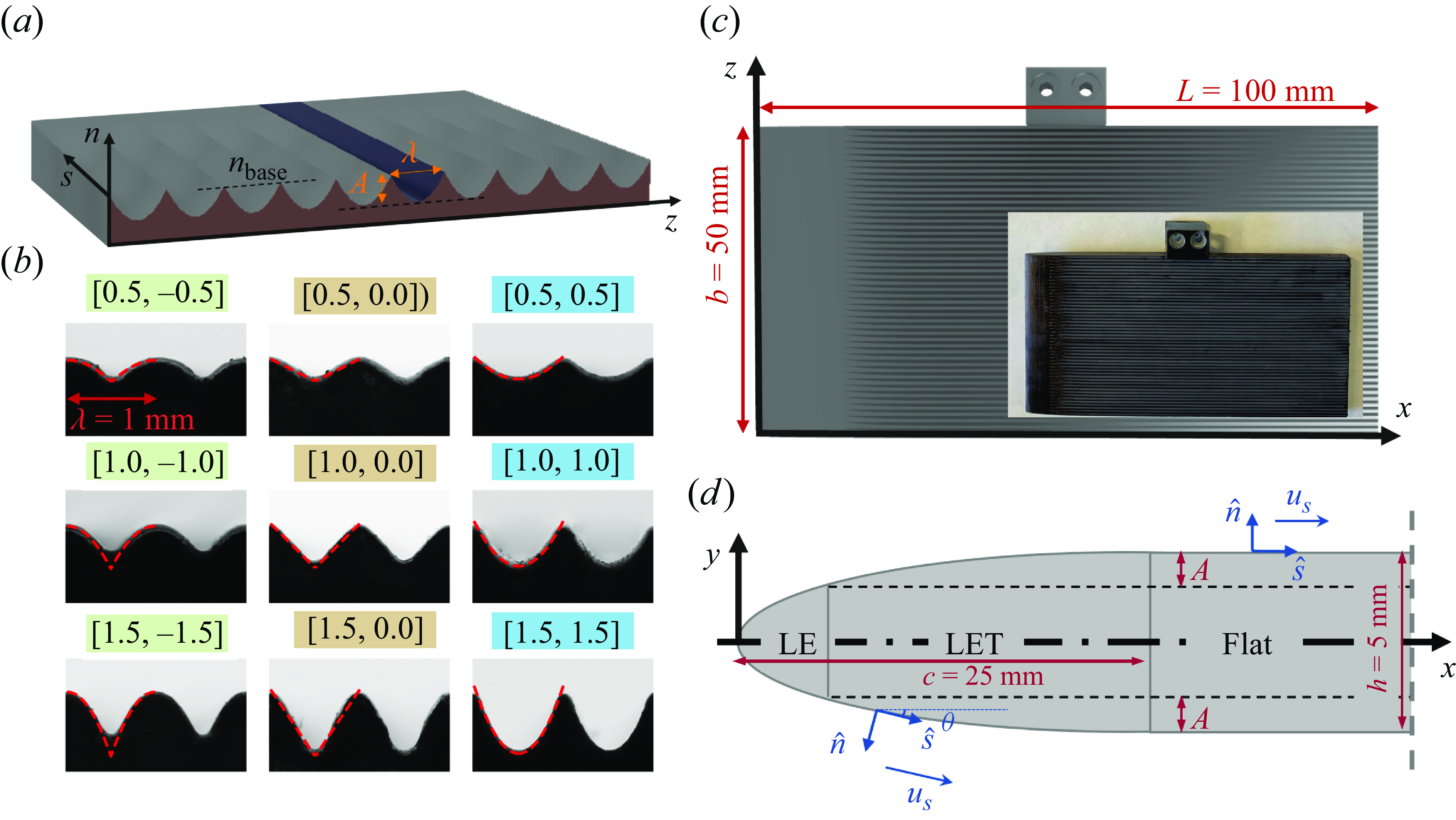
Figure 1. (a) Schematic of a riblet surface with spacing $\lambda$
and height
$\lambda$
and height $A$
and a concave cross-sectional profile. (b) Images of the cross-sectional profiles of the riblet samples. For all the samples,
$A$
and a concave cross-sectional profile. (b) Images of the cross-sectional profiles of the riblet samples. For all the samples, $\lambda = 1$
mm and the respective [
$\lambda = 1$
mm and the respective [ ${\mathcal {R}}, \kappa _2$
] values are listed above each sample. (c) Schematic of the textured sample design and the front view of an actual sample. (d) Schematic of the side view of the sample, including the leading edge of the textured samples and the early part of the Flat region. Three regions, LE, LET and Flat, are shown in the figure as well as the local streamwise and normal directions,
${\mathcal {R}}, \kappa _2$
] values are listed above each sample. (c) Schematic of the textured sample design and the front view of an actual sample. (d) Schematic of the side view of the sample, including the leading edge of the textured samples and the early part of the Flat region. Three regions, LE, LET and Flat, are shown in the figure as well as the local streamwise and normal directions, $\hat {s}$
and
$\hat {s}$
and $\hat {n}$
, on either side of the sample. The dashed line corresponds to the location of the trough of the riblets.
$\hat {n}$
, on either side of the sample. The dashed line corresponds to the location of the trough of the riblets.
-
(i) We focus on the riblets on both sides of a finite-sized symmetric hydrofoil operated at global Reynolds numbers of $\textit{Re}_{L} = 12\,200$
,
$18\,500$
and
$24\,200$
where the flow can remain laminar.
$\textit{Re}_{L} = 12\,200$
,
$18\,500$
and
$24\,200$
where the flow can remain laminar. -
(ii) We take a bio-inspired approach following the pattern of the ribs on the nose of a shark (Lauder et al. Reference Lauder, Wainwright, Domel, Weaver, Wen and Bertoldi2016), and design the riblets to grow from zero height to full size within the curved leading edge of the foil.
-
(iii) We take advantage of the advances in three-dimensional printing techniques in the past decade and print riblets of different cross-sectional shapes embedded on both sides of the foil to have access to drag-reducing, drag-increasing and drag-neutral cases.
-
(iv) To capture the full picture of the flow field around a riblet-covered finite-sized foil, we step away from the earlier experimental formats and use a combined PIV with load measurements. We evaluate both the local and global performance of the riblets and their effect on the development of the BLs, modulating the skin-friction coefficient, and the components of the drag force all compared with a smooth reference.
-
(v) We use the measurements to evaluate the impact of drag-reducing riblet surfaces on the pressure drag and confirm the recently presented numerical evidence for this trend (Mele et al. Reference Mele, Tognaccini and Catalano2016, Reference Mele, Tognaccini, Catalano and de Rosa2020).


This paper is thus organised as follows. In § 2 we discuss the design of the riblets and samples, as well as the experimental procedure and data analysis. In § 3 we first explore the global performance of the riblets in terms of the total drag and then take advantage of a three-tiered force measurement technique to decompose the total drag in terms of friction and pressure drag, as well as contribution from other factors not considered here. We discuss the differences as a function of the shape and size of the riblets (this work is not focused on optimisation of the riblet shapes). Finally, we investigate the local flow behaviour in the presence of the riblets and how the local shear stress and pressure distributions affect the global drag force experienced by the riblet-covered samples. In § 4 we provide a summary of our findings and outline how this localised view of the flow can be used to enhance the designs of drag-reducing riblets for smaller vehicles including the potential for optimisation of the shape of the riblets based on this localised view in the future.
2. Methods
2.1. Riblet geometry
For symmetric and periodic riblets, the shape of the cross-sectional profile of the riblets can be defined only for half of each unit that is mirrored and then repeated as needed. Here, we focus on the simplest family of curved riblets defined using a second-order polynomial (Raayai-Ardakani Reference Raayai-Ardakani2022), where for a unit element with spacing $\lambda$
and height
$\lambda$
and height $A$
(figure 1
a),
$A$
(figure 1
a),
 \begin{align} \frac {n_{w}}{\lambda /2} = \kappa _2\left (\frac {z}{\lambda /2}\right )^{2}+(-\mathcal{R}-\kappa _2)\left (\frac {z}{\lambda /2}\right )+ \dfrac {n_{base}}{\lambda /2} ,\quad 0\leqslant z \leqslant \left(\dfrac {\lambda }{2}\right), \end{align}
where $n_{w}$
is the cross-sectional profile of the riblet wall in the normal direction,
$n_{w}$
is the cross-sectional profile of the riblet wall in the normal direction, $z$
is the spanwise coordinate,
$z$
is the spanwise coordinate, $n_{\textit{base}}$
is the height of the surface that the textures are carved from (equal to the height of the peaks of the textures),
$n_{\textit{base}}$
is the height of the surface that the textures are carved from (equal to the height of the peaks of the textures), ${\mathcal {R}} = A/(\lambda /2)$
is the height-to-half-spacing ratio as a measure of sharpness (Raayai-Ardakani & McKinley Reference Raayai-Ardakani and McKinley2017, Reference Raayai-Ardakani and McKinley2019, Reference Raayai-Ardakani and McKinley2020; Raayai-Ardakani Reference Raayai-Ardakani2022) and
${\mathcal {R}} = A/(\lambda /2)$
is the height-to-half-spacing ratio as a measure of sharpness (Raayai-Ardakani & McKinley Reference Raayai-Ardakani and McKinley2017, Reference Raayai-Ardakani and McKinley2019, Reference Raayai-Ardakani and McKinley2020; Raayai-Ardakani Reference Raayai-Ardakani2022) and $\kappa _2$
is a dimensionless curvature parameter (Raayai-Ardakani Reference Raayai-Ardakani2022). Within this framework,
$\kappa _2$
is a dimensionless curvature parameter (Raayai-Ardakani Reference Raayai-Ardakani2022). Within this framework, $\vert \kappa _2 \vert \leqslant {\mathcal {R}}$
, where
$\vert \kappa _2 \vert \leqslant {\mathcal {R}}$
, where $\kappa _2\lt 0$
corresponds to convex textures,
$\kappa _2\lt 0$
corresponds to convex textures, $\kappa _2\gt 0$
corresponds to concave textures and
$\kappa _2\gt 0$
corresponds to concave textures and $\kappa _2 = 0$
places the commonly used triangular (V-groove) textures as a subset of this riblet family. We focus on the case of textures with
$\kappa _2 = 0$
places the commonly used triangular (V-groove) textures as a subset of this riblet family. We focus on the case of textures with $\lambda = 1$
mm and three height-to-half-spacing ratios of 0.5, 1.0 and 1.5, and one concave (
$\lambda = 1$
mm and three height-to-half-spacing ratios of 0.5, 1.0 and 1.5, and one concave ( $\kappa _2 = {\mathcal {R}}$
), one convex (
$\kappa _2 = {\mathcal {R}}$
), one convex ( $\kappa _2 = -{\mathcal {R}}$
) and one triangular case within each family (nine different textures; see figure 1
b). Throughout this paper, the samples are identified using the vector
$\kappa _2 = -{\mathcal {R}}$
) and one triangular case within each family (nine different textures; see figure 1
b). Throughout this paper, the samples are identified using the vector $\boldsymbol{\kappa } = [ {\mathcal {R}}, \kappa _2]$
. We expect to see a range of drag-reducing, drag-increasing and drag-neutral responses based on the limited previous reports (Walsh & Lindemann Reference Walsh and Lindemann1984; Raayai-Ardakani Reference Raayai-Ardakani2022).
$\boldsymbol{\kappa } = [ {\mathcal {R}}, \kappa _2]$
. We expect to see a range of drag-reducing, drag-increasing and drag-neutral responses based on the limited previous reports (Walsh & Lindemann Reference Walsh and Lindemann1984; Raayai-Ardakani Reference Raayai-Ardakani2022).
Here, we use the variable $s$
and
$s$
and $n$
as the local coordinate system, tangential and normal to the surface (figure 1
d), and use the variable
$n$
as the local coordinate system, tangential and normal to the surface (figure 1
d), and use the variable $\lambda$
instead of the commonly used
$\lambda$
instead of the commonly used $s$
for spacing of the riblets. In addition, we reserve the variable
$s$
for spacing of the riblets. In addition, we reserve the variable $t$
for time and use
$t$
for time and use $h$
for the thickness of the finite-sized samples and employ
$h$
for the thickness of the finite-sized samples and employ $A$
instead of
$A$
instead of $h$
for the height of the riblet units. These simple changes compared with the commonly used variables allow us to avoid confusion. In addition, we use the word ‘smooth’ as the opposite of a riblet surface while we use the word ‘flat’ as opposed to a ‘curved’ surface.
$h$
for the height of the riblet units. These simple changes compared with the commonly used variables allow us to avoid confusion. In addition, we use the word ‘smooth’ as the opposite of a riblet surface while we use the word ‘flat’ as opposed to a ‘curved’ surface.
2.2. Textured samples
We use fully textured samples where the riblets are fabricated seamlessly with the samples. The base of the samples has the form of a symmetric slender plate, comprised of a leading edge, and a main body (100 mm in length (L), 50 mm in width (b) and 5 mm in depth (h)). The leading edge is streamlined in the form of an ellipse (similar to the design used by Fu & Raayai-Ardakani Reference Fu and Raayai-Ardakani2023) up to $x=25 \ \textrm { mm}$
where it asymptotically meets a flat main body that extends to a blunt trailing edge (
$x=25 \ \textrm { mm}$
where it asymptotically meets a flat main body that extends to a blunt trailing edge ( $25\,\textrm{mm} \leqslant x \leqslant 100 \ \textrm { mm}$
; see figure 1
c). The riblets are carved out of the base geometry on both sides of the sample. In this case, with the coordinate system shown in figure 1(c–d), the base height in the main (Flat) region of the body,
$25\,\textrm{mm} \leqslant x \leqslant 100 \ \textrm { mm}$
; see figure 1
c). The riblets are carved out of the base geometry on both sides of the sample. In this case, with the coordinate system shown in figure 1(c–d), the base height in the main (Flat) region of the body, $\vert y_{\textit{base}} \vert$
, is at half of the thickness,
$\vert y_{\textit{base}} \vert$
, is at half of the thickness, $h/2$
, on either side. The peaks of the textures reside at this height on either side and the troughs are located at
$h/2$
, on either side. The peaks of the textures reside at this height on either side and the troughs are located at $\vert y_{\textit{base}} \vert - A$
. However, this is only true for the Flat region of the sample within (
$\vert y_{\textit{base}} \vert - A$
. However, this is only true for the Flat region of the sample within ( $25 \ \textrm { mm} \leqslant x \leqslant 100 \ \textrm { mm}$
) and prior to that, due to the curved nature of the leading edge, the textures appear where there is enough thickness (see figure 1
c–d) and grow to their maximum height
$25 \ \textrm { mm} \leqslant x \leqslant 100 \ \textrm { mm}$
) and prior to that, due to the curved nature of the leading edge, the textures appear where there is enough thickness (see figure 1
c–d) and grow to their maximum height $A$
at the end of the elliptical leading edge. We call this region ‘leading edge textured’(LET) and the non-riblet segment of the leading edge as LE. At the leading edge of fully riblet-covered flat plates, for at least
$A$
at the end of the elliptical leading edge. We call this region ‘leading edge textured’(LET) and the non-riblet segment of the leading edge as LE. At the leading edge of fully riblet-covered flat plates, for at least $x/\lambda \lt 9$
, riblets experience larger spanwise-averaged wall shear (normalised with
$x/\lambda \lt 9$
, riblets experience larger spanwise-averaged wall shear (normalised with $\lambda$
) compared with the smooth reference (Raayai-Ardakani & McKinley Reference Raayai-Ardakani and McKinley2017), and to mitigate that, we mimic the distribution of the denticles on the nose of sharks (Lauder et al. Reference Lauder, Wainwright, Domel, Weaver, Wen and Bertoldi2016) (which start from smooth in the nose area with ribs appearing later along the body) in the design of the streamlined leading edge of the samples. Thus, instead of enforcing a constant height-to-half-spacing ratio for the textures, we keep the wavelength constant and let the height of the textures grow from zero to the final height,
$\lambda$
) compared with the smooth reference (Raayai-Ardakani & McKinley Reference Raayai-Ardakani and McKinley2017), and to mitigate that, we mimic the distribution of the denticles on the nose of sharks (Lauder et al. Reference Lauder, Wainwright, Domel, Weaver, Wen and Bertoldi2016) (which start from smooth in the nose area with ribs appearing later along the body) in the design of the streamlined leading edge of the samples. Thus, instead of enforcing a constant height-to-half-spacing ratio for the textures, we keep the wavelength constant and let the height of the textures grow from zero to the final height, $A$
, at the end of the elliptic area and let the BL evolve with the evolution of the riblets.
$A$
, at the end of the elliptic area and let the BL evolve with the evolution of the riblets.
Riblet samples (and one smooth for comparison) are three-dimensionally printed (Formlabs Form3 3D printer and a photo-polymer resin, figure 1
b--c). After printing, the spacing and height of the riblets are measured using Bruker ContourX-500 Optical Profilometer and analysed with the open-source software package Gwyddion. The measurements are conducted at four different random locations on each side of the samples, with each location covering about $2.8\ \textrm { mm}^{2}$
of the projected area and containing at least one riblet unit, and the mean of the measurements and their
$2.8\ \textrm { mm}^{2}$
of the projected area and containing at least one riblet unit, and the mean of the measurements and their $95\, \%$
confidence intervals are reported in table 1. Owing to the limited resolution of the three-dimensional printer, the final height of the riblets are smaller than the design heights and result in lower apparent
$95\, \%$
confidence intervals are reported in table 1. Owing to the limited resolution of the three-dimensional printer, the final height of the riblets are smaller than the design heights and result in lower apparent ${\mathcal {R}}$
values for the samples, but do not affect the performance of the riblets. Throughout the paper the samples are identified with their design names as listed in the first column of table 1. Even though the experiments are limited to the laminar regime, for completeness, the distributions of the spacing and height of the riblets in wall units are presented in figures 2 and SI.1 of the supplementary material, calculated based on the spanwise-averaged shear stress distribution (discussed in § 3.3). Except for the non-textured leading edge region of the samples,
${\mathcal {R}}$
values for the samples, but do not affect the performance of the riblets. Throughout the paper the samples are identified with their design names as listed in the first column of table 1. Even though the experiments are limited to the laminar regime, for completeness, the distributions of the spacing and height of the riblets in wall units are presented in figures 2 and SI.1 of the supplementary material, calculated based on the spanwise-averaged shear stress distribution (discussed in § 3.3). Except for the non-textured leading edge region of the samples, $\lambda ^{+}$
is less than
$\lambda ^{+}$
is less than $24-25$
for all the samples and on both sides, which coincides with the ranges previously identified as drag-reducing (Walsh Reference Walsh1983; Walsh & Lindemann Reference Walsh and Lindemann1984; Bechert et al. Reference Bechert, Bruse, Hage, Van der Hoeven and Hoppe1997).
$24-25$
for all the samples and on both sides, which coincides with the ranges previously identified as drag-reducing (Walsh Reference Walsh1983; Walsh & Lindemann Reference Walsh and Lindemann1984; Bechert et al. Reference Bechert, Bruse, Hage, Van der Hoeven and Hoppe1997).
Table 1. Details of the geometry of the riblets and set-up. The locations of the start of the textures ( $x_{{ LET}}$
) are measured using a caliper (design values in the parenthesis).
$x_{{ LET}}$
) are measured using a caliper (design values in the parenthesis).

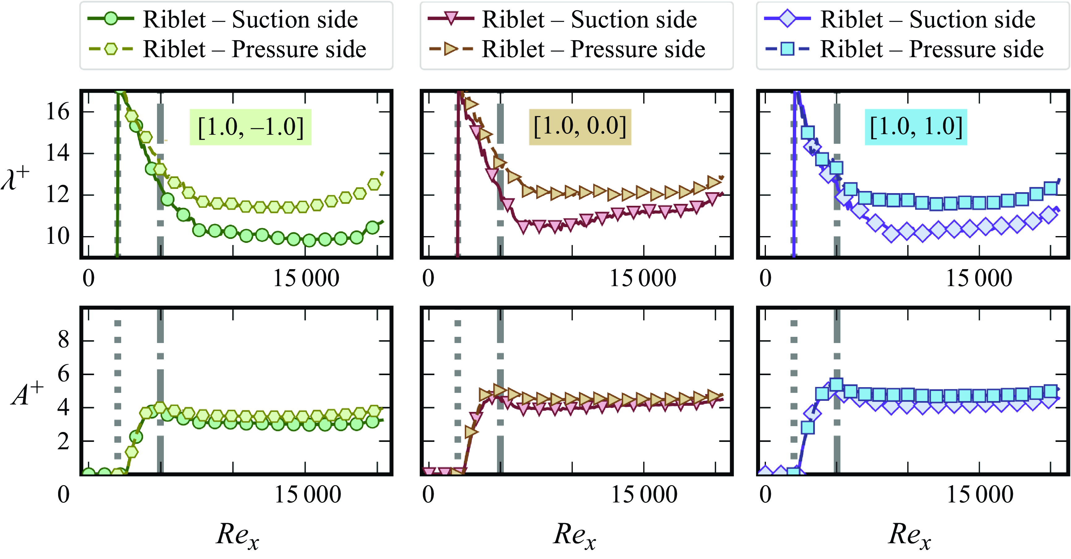
Figure 2. Distribution of $\lambda ^{+}$
and
$\lambda ^{+}$
and $A^{+}$
for all the riblet samples with
$A^{+}$
for all the riblet samples with ${\mathcal {R}} = 1.0$
on the suction and pressure side for
${\mathcal {R}} = 1.0$
on the suction and pressure side for $\textit{Re}_{L} = 18\,500$
, calculated using the spanwise-averaged shear stress measured (presented in § 3.3). Each column corresponds to specific samples. Locations of
$\textit{Re}_{L} = 18\,500$
, calculated using the spanwise-averaged shear stress measured (presented in § 3.3). Each column corresponds to specific samples. Locations of $x_{ LET}$
and
$x_{ LET}$
and $x_{Flat}$
are marked by grey dotted and dash-dotted vertical lines.
$x_{Flat}$
are marked by grey dotted and dash-dotted vertical lines.
2.3. Experimental procedure
Experiments are performed following the procedure described previously (Fu & Raayai-Ardakani Reference Fu and Raayai-Ardakani2023; Fu et al. Reference Fu and Raayai-Ardakani2023). In summary, the samples described in § 2.2 are attached to a dynamometer consisting of linear variable differential transformers (to measure the total drag force) and suspended in a water tunnel (cross-sectional area of $20 \times 20 \ \textrm { cm}$
and
$20 \times 20 \ \textrm { cm}$
and $2 \ \textrm { m}$
in length; see figure 3). The samples are positioned at around
$2 \ \textrm { m}$
in length; see figure 3). The samples are positioned at around $75 \ \textrm { cm}$
from the tunnel entrance and close to the middle of the cross-section to reduce the effects of the tunnel walls on the measurements. The experiments are performed at three free-stream velocities less than
$75 \ \textrm { cm}$
from the tunnel entrance and close to the middle of the cross-section to reduce the effects of the tunnel walls on the measurements. The experiments are performed at three free-stream velocities less than $0.25 \ \textrm {m s}^{-1}$
(
$0.25 \ \textrm {m s}^{-1}$
( $0.122$
,
$0.122$
, $0.185$
and
$0.185$
and $0.242 \ \textrm { m s}^{-1}$
) corresponding to global Reynolds numbers,
$0.242 \ \textrm { m s}^{-1}$
) corresponding to global Reynolds numbers, $\textit{Re}_{L} = \rho U_{\infty }L/\mu$
, of 12,200, 18,500 and 24,200 (turbulence intensity of the free stream is less than or about
$\textit{Re}_{L} = \rho U_{\infty }L/\mu$
, of 12,200, 18,500 and 24,200 (turbulence intensity of the free stream is less than or about $1\, \%$
).
$1\, \%$
).
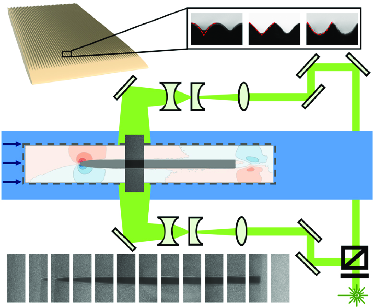
The velocity field all around the sample is captured using a double-pulsed planar (two-dimensional, two-component, 2D-2C) PIV and double-illumination, consecutive-overlapping procedure (Fu & Raayai-Ardakani Reference Fu and Raayai-Ardakani2023; Fu et al. Reference Fu and Raayai-Ardakani2023). The set-up is comprised of a double-pulsed Nd:YAG laser operated at $15 \ \textrm { Hz}$
repetition rate and the nominal output energies of
$15 \ \textrm { Hz}$
repetition rate and the nominal output energies of $10 \ \textrm { mJ}$
or
$10 \ \textrm { mJ}$
or $20 \ \textrm { mJ}$
per pulse for different free-stream velocities. The high-speed camera is set to a resolution of 720
$20 \ \textrm { mJ}$
per pulse for different free-stream velocities. The high-speed camera is set to a resolution of 720 $\times$
1920 pixels and the timing between the two consecutive pulses is adjusted to
$\times$
1920 pixels and the timing between the two consecutive pulses is adjusted to $\delta t =1000$ $\unicode {x03BC}$
s for free-stream velocities of 0.122 m s
$\unicode {x03BC}$
s for free-stream velocities of 0.122 m s $^{-1}$
and 0.185 m s–1, and
$^{-1}$
and 0.185 m s–1, and $\delta t =$
900
$\delta t =$
900 $\unicode {x03BC}$
s for 0.242 m s–1 to allow for the slowest particles to have visible movement and the fastest particles to not move beyond half of the PIV analysis window (set at 32 pixels).
$\unicode {x03BC}$
s for 0.242 m s–1 to allow for the slowest particles to have visible movement and the fastest particles to not move beyond half of the PIV analysis window (set at 32 pixels).
To get simultaneous access to both sides of a non-transparent sample and avoid any assumptions regarding the symmetry of the flow around the foils, we use a double-illumination strategy (Fu & Raayai-Ardakani Reference Fu and Raayai-Ardakani2023; Fu et al. Reference Fu and Raayai-Ardakani2023). This optical set-up is comprised of a half-wave plate and a polarising beam splitter to divide the incoming laser into two almost equal beams. These beams are then guided toward either side of the sample through additional mirrors where two combinations of light-sheet optics, involving two spherical lenses and one cylindrical lens, are positioned on opposite sides of the water tunnel to create light sheets with thicknesses of about $ 1 \ \textrm { mm}$
.
$ 1 \ \textrm { mm}$
.
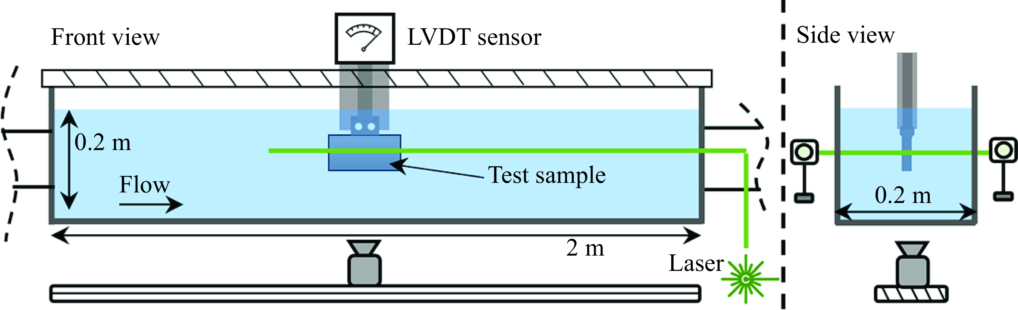
Figure 3. Schematic of the experimental set-up, showing front and side views of the water tunnel, the installed sample and the PIV set-up.
To have access to the velocity field in both the BL and the far field, we use a consecutive-overlapping imaging procedure (Fu & Raayai-Ardakani Reference Fu and Raayai-Ardakani2023; Fu et al. Reference Fu and Raayai-Ardakani2023). We attach the camera to a CNC rail and traverse the entire area of interest of the flow with about $40\, \%\!-\!45\,\%$
overlap between the fields of views. To have access to the velocity profiles in the BL, we use a magnification of 1 px
$40\, \%\!-\!45\,\%$
overlap between the fields of views. To have access to the velocity profiles in the BL, we use a magnification of 1 px $\equiv$
15–16
$\equiv$
15–16 $\unicode {x03BC}\textrm {m}$
that limits the total field of view of the camera at a time and the consecutive-overlapping imaging allows us to overcome this limitation and capture a larger area of interest. Here we use a one-dimensional sweep in the streamwise direction, with 36 overlapping steps to capture a span of about 180
$\unicode {x03BC}\textrm {m}$
that limits the total field of view of the camera at a time and the consecutive-overlapping imaging allows us to overcome this limitation and capture a larger area of interest. Here we use a one-dimensional sweep in the streamwise direction, with 36 overlapping steps to capture a span of about 180 $\textrm {mm}$
in the streamwise direction and about 25 mm in the normal direction. On either side, the BL thickness does not go beyond 3 mm.
$\textrm {mm}$
in the streamwise direction and about 25 mm in the normal direction. On either side, the BL thickness does not go beyond 3 mm.
At each step, 50 image pairs are captured. Fu & Raayai-Ardakani (Reference Fu and Raayai-Ardakani2023) have previously shown that 50 image pairs are enough for the measurements to reach convergence in a similar range of Reynolds number as that used here. The images (and subsequently the analysed velocity fields) are then stitched together based on the global locations of the camera as controlled with the CNC rail. The PIV images at each step of imaging are analysed using an in-house Python script utilising the open-source software OpenPIV (Liberzon et al. Reference Liberzon2020) (with $32 \times 32$
windows and a search area of
$32 \times 32$
windows and a search area of $64 \times 64$
with
$64 \times 64$
with $85\, \%$
overlap) to find the velocity in the
$85\, \%$
overlap) to find the velocity in the $x$
and
$x$
and $y$
directions (
$y$
directions ( $u$
and
$u$
and $v$
, respectively) with an additional correction loop for the velocities close to the wall region (Fu & Raayai-Ardakani Reference Fu and Raayai-Ardakani2023) to avoid bias errors due to the large shear rates close to the walls (Kähler, Scharnowski & Cierpka Reference Kähler, Scharnowski and Cierpka2012).
$v$
, respectively) with an additional correction loop for the velocities close to the wall region (Fu & Raayai-Ardakani Reference Fu and Raayai-Ardakani2023) to avoid bias errors due to the large shear rates close to the walls (Kähler, Scharnowski & Cierpka Reference Kähler, Scharnowski and Cierpka2012).
2.4. Data analysis
2.4.1. Angle of attack
While each sample is positioned as close to parallel to the streamwise direction as possible, there is always the potential for a slight non-zero angle of attack, $\alpha$
, not visible to the naked eye in the set-up and the final angle of attack of the sample with respect to the free-stream velocity is not known a priori. This
$\alpha$
, not visible to the naked eye in the set-up and the final angle of attack of the sample with respect to the free-stream velocity is not known a priori. This $\alpha$
results in an asymmetry in the flow and subsequently differences between the local responses of the front (
$\alpha$
results in an asymmetry in the flow and subsequently differences between the local responses of the front ( $y\gt 0$
) and back (
$y\gt 0$
) and back ( $y\lt 0$
) sides of the samples. To find this angle of attack more accurately for each of the experiments, we use the velocity field upstream of the leading edge and a potential model of flow past an elliptical leading edge (previously described by Fu & Raayai-Ardakani Reference Fu and Raayai-Ardakani2023) and fit the velocity measurements to the potential model to find the
$y\lt 0$
) sides of the samples. To find this angle of attack more accurately for each of the experiments, we use the velocity field upstream of the leading edge and a potential model of flow past an elliptical leading edge (previously described by Fu & Raayai-Ardakani Reference Fu and Raayai-Ardakani2023) and fit the velocity measurements to the potential model to find the $\alpha$
between the sample and the free-stream velocity, as listed in the last column of table 1. Since the experiments with each sample were performed in one session (only changing the velocity), the values of the
$\alpha$
between the sample and the free-stream velocity, as listed in the last column of table 1. Since the experiments with each sample were performed in one session (only changing the velocity), the values of the $\alpha$
are a mean of fits at 30 locations within
$\alpha$
are a mean of fits at 30 locations within $x/L\lt -0.14$
of the leading edge and for all the threeruns (different
$x/L\lt -0.14$
of the leading edge and for all the threeruns (different $\textit{Re}_L$
) of each sample for a total of 90 values. Owing to the angle of attack, and with the geometric configuration of the experimental set-up, the front/back sides of the samples coincide with the suction/pressure sides of the foils, respectively.
$\textit{Re}_L$
) of each sample for a total of 90 values. Owing to the angle of attack, and with the geometric configuration of the experimental set-up, the front/back sides of the samples coincide with the suction/pressure sides of the foils, respectively.
2.4.2. Shear stress distribution
To calculate the local shear stress distribution, we employ the PIV data to find the velocity profiles at each $x$
location and calculate the local velocity gradient normal to the wall as a function of the local Reynolds number,
$x$
location and calculate the local velocity gradient normal to the wall as a function of the local Reynolds number, $\textit{Re}_x = \rho U(x) x/\mu$
, where
$\textit{Re}_x = \rho U(x) x/\mu$
, where $U(x)$
is the velocity at the edge of the BL. Numerical simulations of a BL over riblet surfaces (Choi et al. Reference Choi, Moin and Kim1993; Goldstein et al. Reference Goldstein, Handler and Sirovich1995; Raayai-Ardakani & McKinley Reference Raayai-Ardakani and McKinley2017, Reference Raayai-Ardakani and McKinley2020) have previously shown that in the presence of the riblets, the velocity profiles are dependent on all three dimensions,
$U(x)$
is the velocity at the edge of the BL. Numerical simulations of a BL over riblet surfaces (Choi et al. Reference Choi, Moin and Kim1993; Goldstein et al. Reference Goldstein, Handler and Sirovich1995; Raayai-Ardakani & McKinley Reference Raayai-Ardakani and McKinley2017, Reference Raayai-Ardakani and McKinley2020) have previously shown that in the presence of the riblets, the velocity profiles are dependent on all three dimensions, $\mathbf{u}(x,y,z)$
, and dependent on the spanwise direction,
$\mathbf{u}(x,y,z)$
, and dependent on the spanwise direction, $z$
, in a periodic manner. This is directly a result of the shape of the riblet surface and the no-slip wall. However, the previous numerical and experimental observations (Djenidi et al. Reference Djenidi, Liandrat, Anselmet and Fulachier1989, Reference Djenidi, Anselmet, Liandrat and Fulachier1994; Choi et al. Reference Choi, Moin and Kim1993; Djenidi & Antonia Reference Djenidi and Antonia1996; Raayai-Ardakani & McKinley Reference Raayai-Ardakani and McKinley2017, Reference Raayai-Ardakani and McKinley2019, Reference Raayai-Ardakani and McKinley2020) all show that the spatial variations in the velocity profiles are dominant inside the riblet unit element. While moving outside the grooves, all velocity profiles at a given
$z$
, in a periodic manner. This is directly a result of the shape of the riblet surface and the no-slip wall. However, the previous numerical and experimental observations (Djenidi et al. Reference Djenidi, Liandrat, Anselmet and Fulachier1989, Reference Djenidi, Anselmet, Liandrat and Fulachier1994; Choi et al. Reference Choi, Moin and Kim1993; Djenidi & Antonia Reference Djenidi and Antonia1996; Raayai-Ardakani & McKinley Reference Raayai-Ardakani and McKinley2017, Reference Raayai-Ardakani and McKinley2019, Reference Raayai-Ardakani and McKinley2020) all show that the spatial variations in the velocity profiles are dominant inside the riblet unit element. While moving outside the grooves, all velocity profiles at a given $x$
location collapse onto each other with no spanwise dependence visible.
$x$
location collapse onto each other with no spanwise dependence visible.
In planar PIV the flow measurements performed in the thin plane of the light sheet are an average of the velocity field within this light sheet. Thus, in our current experiments, we set the thickness of the light sheet to about 1 mm to match the spacing of one riblet unit and ensure the depth of field of the camera is also around 1 mm to capture a spanwise-averaged velocity measurement. Writing the velocity profile as $\mathbf{u}(x,y,z)$
, the measured velocity profile is then
$\mathbf{u}(x,y,z)$
, the measured velocity profile is then $\langle \mathbf{u} \rangle (x,y)$
, where
$\langle \mathbf{u} \rangle (x,y)$
, where $\langle \cdots \rangle (x,y)$
denotes the spanwise-averaging operation. Owing to the opaqueness of the samples, only the velocity distribution outside of the grooves (
$\langle \cdots \rangle (x,y)$
denotes the spanwise-averaging operation. Owing to the opaqueness of the samples, only the velocity distribution outside of the grooves ( $n\gt 0$
) is visible to the camera, and the rest of the profiles have their respective no-slip wall hidden inside the grooves, below the level accessible to imaging. Thus, the origin of the average velocity
$n\gt 0$
) is visible to the camera, and the rest of the profiles have their respective no-slip wall hidden inside the grooves, below the level accessible to imaging. Thus, the origin of the average velocity $\langle \mathbf{u} \rangle$
is located below the peak of the riblets (
$\langle \mathbf{u} \rangle$
is located below the peak of the riblets ( $n\lt 0$
). We use this origin as a representative average origin of the velocity within one texture unit and denote it as the ‘effective origin’ of the riblets,
$n\lt 0$
). We use this origin as a representative average origin of the velocity within one texture unit and denote it as the ‘effective origin’ of the riblets, $n_0$
.
$n_0$
.
From the PIV data, we calculate the spanwise-averaged velocity gradient and subsequently the local spanwise-averaged shear stress, $\langle \tau \rangle = \mu \partial \langle u_{s} \rangle /\partial n$
. Instead of depending on only a few measurement points close to the wall, we use as many of the measured velocity points as possible and characterise the velocity profiles in a mathematical format and fit the profiles to an appropriate functional form. Here, we employ an updated form of the Falkner–Skan (FS) (Falkner & Skan Reference Falkneb and Skan1931) family of BLs in a localised manner to capture the behaviour of the tangential velocity, denoted by
$\langle \tau \rangle = \mu \partial \langle u_{s} \rangle /\partial n$
. Instead of depending on only a few measurement points close to the wall, we use as many of the measured velocity points as possible and characterise the velocity profiles in a mathematical format and fit the profiles to an appropriate functional form. Here, we employ an updated form of the Falkner–Skan (FS) (Falkner & Skan Reference Falkneb and Skan1931) family of BLs in a localised manner to capture the behaviour of the tangential velocity, denoted by $\langle u_{s} \rangle = \langle u \rangle \cos \theta + \langle v \rangle \sin \theta$
(where
$\langle u_{s} \rangle = \langle u \rangle \cos \theta + \langle v \rangle \sin \theta$
(where $\theta$
is the local angle between
$\theta$
is the local angle between $\hat {s}$
and
$\hat {s}$
and $x$
directions). In this updated formulation, we define
$x$
directions). In this updated formulation, we define $\langle u_{s} \rangle$
as a function of the local Reynolds number,
$\langle u_{s} \rangle$
as a function of the local Reynolds number, $\textit{Re}_{x} = {\rho x U(x)}/{\mu }$
,
$\textit{Re}_{x} = {\rho x U(x)}/{\mu }$
, $n$
,
$n$
, $m$
, and the effective origin
$m$
, and the effective origin $n_0$
, in the form of
$n_0$
, in the form of $\langle u_{s} \rangle = \mathcal{H}(\textit{Re}_{x},n;m,n_{0})$
, where the averaged velocity profile is a function of an updated similarity variable
$\langle u_{s} \rangle = \mathcal{H}(\textit{Re}_{x},n;m,n_{0})$
, where the averaged velocity profile is a function of an updated similarity variable $\eta ^*$
, of the form
$\eta ^*$
, of the form ${\langle u_{s}\rangle }/{U} = \mathcal{F}^{\prime}(\eta ^{*})$
with
${\langle u_{s}\rangle }/{U} = \mathcal{F}^{\prime}(\eta ^{*})$
with $\eta ^{*}$
defined as
$\eta ^{*}$
defined as
 \begin{align} \eta ^{*} = \dfrac {(n-n_{0})}{x} \sqrt {\textit{Re}_x\left (\dfrac {m+1}{2}\right )}. \end{align}
Now, with this formulation, and the experimental data for $\langle u_{s} \rangle$
, the local normal direction,
$\langle u_{s} \rangle$
, the local normal direction, $n$
, and
$n$
, and $\textit{Re}_x$
, we locally fit the data to the FS solutions to the BL equations and find the best values of
$\textit{Re}_x$
, we locally fit the data to the FS solutions to the BL equations and find the best values of $m$
and
$m$
and $n_0$
that capture the profiles at every location. A few examples of the fitted velocities along the suction side of the [1.0, 0.0] sample operated at
$n_0$
that capture the profiles at every location. A few examples of the fitted velocities along the suction side of the [1.0, 0.0] sample operated at $\textit{Re}_{L} = 18\,500$
are shown in figure SI.2(a) of the supplementary material. In the curved leading edge area (LE and LET),
$\textit{Re}_{L} = 18\,500$
are shown in figure SI.2(a) of the supplementary material. In the curved leading edge area (LE and LET), $n \nparallel y$
, and for simplicity, instead of
$n \nparallel y$
, and for simplicity, instead of $s$
we use
$s$
we use $x$
and
$x$
and $\textit{Re}_x$
to characterise the streamwise velocity profiles (with every
$\textit{Re}_x$
to characterise the streamwise velocity profiles (with every $x$
having a unique mapping to
$x$
having a unique mapping to $s$
and vice versa, we let the marginal effect of the difference between the magnitude of
$s$
and vice versa, we let the marginal effect of the difference between the magnitude of $s$
and
$s$
and $x$
be captured in the
$x$
be captured in the $m$
parameter). The first reliable fit is around
$m$
parameter). The first reliable fit is around $x=1 \ \textrm { mm}$
where
$x=1 \ \textrm { mm}$
where $s/x \approx 1.27$
and by the end of the LET
$s/x \approx 1.27$
and by the end of the LET $s/x \approx 1 .015$
. In the Flat region, the streamwise and normal direction align with
$s/x \approx 1 .015$
. In the Flat region, the streamwise and normal direction align with $x$
and
$x$
and $y$
coordinates (
$y$
coordinates ( $\langle u_{s} \rangle = \langle u \rangle )$
.
$\langle u_{s} \rangle = \langle u \rangle )$
.
Note that due to the finite thickness of the sample, the BL edge velocity, $U(x) \geqslant U_{\infty }$
, and, thus, local
$U(x) \geqslant U_{\infty }$
, and, thus, local $\textit{Re}_x$
values are larger than Reynolds numbers calculated using
$\textit{Re}_x$
values are larger than Reynolds numbers calculated using $\rho U_{\infty }L/\mu$
and, thus,
$\rho U_{\infty }L/\mu$
and, thus, $\textit{Re}_{x=L}\gt \textit{Re}_{L}$
. Here, we do not find one single
$\textit{Re}_{x=L}\gt \textit{Re}_{L}$
. Here, we do not find one single $m$
for the entire flow, but use this family of FS solutions and the parameter
$m$
for the entire flow, but use this family of FS solutions and the parameter $m$
as mathematical tools to characterise the local behaviour of the flow field, especially including terms that cannot be captured directly with the planar PIV measurements (discussed further in the upcoming § 3.4).
$m$
as mathematical tools to characterise the local behaviour of the flow field, especially including terms that cannot be captured directly with the planar PIV measurements (discussed further in the upcoming § 3.4).
Knowing the mathematical form of the FS solutions as well as the distribution of the $m$
and
$m$
and $n_0$
from the available data, the local spanwise-averaged shear stress distribution along each side of the plate at
$n_0$
from the available data, the local spanwise-averaged shear stress distribution along each side of the plate at $n=0$
is found as
$n=0$
is found as
 \begin{align} \langle \tau _{n=0} \rangle (x) = \mu \left . \dfrac {\partial \langle u_{s} \rangle }{\partial n} \right \vert _{n=0} = \left . \left (\frac {m+1}{2}\right )^{0.5}\frac {\rho U(x)^{2}}{\sqrt {\textit{Re}_x}}\mathcal{F}^{{\prime}{\prime}}\right \vert _{\eta ^{*}=\eta ^{*}_0} ,\end{align}
and the spanwise-averaged skin-friction coefficient is determined by $\langle C_f \rangle (x) = \langle \tau _{n=0} \rangle (x)/{({1}/{2})\rho U(x)^{2}}$
. Since we only have access to the velocity distribution outside the grooves, as written in (2.3), we use the gradient of
$\langle C_f \rangle (x) = \langle \tau _{n=0} \rangle (x)/{({1}/{2})\rho U(x)^{2}}$
. Since we only have access to the velocity distribution outside the grooves, as written in (2.3), we use the gradient of $\langle u_{s} \rangle$
profiles on the
$\langle u_{s} \rangle$
profiles on the $n=0$
plane to find
$n=0$
plane to find $\langle \tau _{n=0} \rangle$
distribution at every location. We show that by using a simple control volume analysis inside the grooves (as discussed in § SI.2 of the supplementary material) the gradient of
$\langle \tau _{n=0} \rangle$
distribution at every location. We show that by using a simple control volume analysis inside the grooves (as discussed in § SI.2 of the supplementary material) the gradient of $\langle u_{s} \rangle$
profiles on the
$\langle u_{s} \rangle$
profiles on the $n=0$
is able to capture the essence of the velocity gradient distribution at the riblet wall while also capturing the effect of the excess wetted surface area of the riblets compared with the smooth reference. We also provide further analysis in § SI.2 ofthe supplementary material on the upper and lower bounds of the difference between
$n=0$
is able to capture the essence of the velocity gradient distribution at the riblet wall while also capturing the effect of the excess wetted surface area of the riblets compared with the smooth reference. We also provide further analysis in § SI.2 ofthe supplementary material on the upper and lower bounds of the difference between $\langle \tau _{{ w}} \rangle$
(which is the spanwise-averaged shear stress on the riblet wall) and
$\langle \tau _{{ w}} \rangle$
(which is the spanwise-averaged shear stress on the riblet wall) and $\langle \tau _{n=0} \rangle$
measured on the
$\langle \tau _{n=0} \rangle$
measured on the $n=0$
plane based on the available PIV measurements. Note, at each local Reynolds number, the direct effect of
$n=0$
plane based on the available PIV measurements. Note, at each local Reynolds number, the direct effect of $n_0$
on the magnitude of the
$n_0$
on the magnitude of the $\langle \tau _{n=0} \rangle$
, as written in (2.3), is mainly hidden in the value of the
$\langle \tau _{n=0} \rangle$
, as written in (2.3), is mainly hidden in the value of the $\eta ^{*}_0$
at the peak of the grooves. We use the
$\eta ^{*}_0$
at the peak of the grooves. We use the $\langle \tau _{n=0} \rangle$
of the riblets and the
$\langle \tau _{n=0} \rangle$
of the riblets and the $\tau _{_{0}}$
of the smooth reference (Fu & Raayai-Ardakani Reference Fu and Raayai-Ardakani2023) as local measures for comparing the frictional (shear) response of the surfaces.
$\tau _{_{0}}$
of the smooth reference (Fu & Raayai-Ardakani Reference Fu and Raayai-Ardakani2023) as local measures for comparing the frictional (shear) response of the surfaces.
2.4.3. Pressure and pressure gradient distribution
We use the PIV data to find the pressure gradient and pressure distribution by using the Reynolds-averaged Navier--Stokes (RANS) equations inthe $x$
and
$x$
and $y$
direction and lineintegration of the gradient terms in those directions (Liu & Katz Reference Liu and Katz2006; Charonko et al. Reference Charonko, King, Smith and Vlachos2010; de Kat & Ganapathisubramani Reference de Kat and Ganapathisubramani2013; van Oudheusden Reference van Oudheusden2013; Liu, Moreto & Siddle-Mitchell Reference Liu, Moreto and Siddle-Mitchell2016; Liu & Moreto Reference Liu and Moreto2020; Nie et al. Reference Nie, Whitehead, Richards, Smith and Pan2022; Fu & Raayai-Ardakani Reference Fu and Raayai-Ardakani2023; Suchandra & Raayai-Ardakani Reference Suchandra and Raayai-Ardakani2024):
$y$
direction and lineintegration of the gradient terms in those directions (Liu & Katz Reference Liu and Katz2006; Charonko et al. Reference Charonko, King, Smith and Vlachos2010; de Kat & Ganapathisubramani Reference de Kat and Ganapathisubramani2013; van Oudheusden Reference van Oudheusden2013; Liu, Moreto & Siddle-Mitchell Reference Liu, Moreto and Siddle-Mitchell2016; Liu & Moreto Reference Liu and Moreto2020; Nie et al. Reference Nie, Whitehead, Richards, Smith and Pan2022; Fu & Raayai-Ardakani Reference Fu and Raayai-Ardakani2023; Suchandra & Raayai-Ardakani Reference Suchandra and Raayai-Ardakani2024):
 \begin{align} \dfrac {\partial p}{\partial x} = \left [ -\rho \left (u \frac {\partial u}{\partial x} + v \frac {\partial u}{\partial y} \right ) + \mu \left ( \frac {\partial ^{2} u}{\partial x^{2}} + \frac {\partial ^{2} u}{\partial y^{2}} \right ) - \rho \left (\frac {\partial \overline {u^{\prime} u^{\prime}}}{\partial x} + \frac {\partial \overline {u^{\prime} v^{\prime}}}{\partial y} \right ) \right ] ,\end{align}
 \begin{align} \dfrac {\partial p}{\partial y} = \left [ -\rho \left (u \frac {\partial v}{\partial x} + v \frac {\partial v}{\partial y} \right ) + \mu \left ( \frac {\partial ^{2} v}{\partial x^{2}} + \frac {\partial ^{2} v}{\partial y^{2}} \right ) - \rho \left (\frac {\partial \overline {u^{\prime} v^{\prime}}}{\partial x} + \frac {\partial \overline {v^{\prime} v^{\prime}}}{\partial y} \right ) \right ]. \\[6pt] \nonumber \end{align}
Here $\rho$
and
$\rho$
and $\mu$
are the fluid’s density and dynamic viscosity, respectively, and
$\mu$
are the fluid’s density and dynamic viscosity, respectively, and $\overline {(\ldots )}$
denotes ensembleaveraging with the instantaneous velocity vector
$\overline {(\ldots )}$
denotes ensembleaveraging with the instantaneous velocity vector ${\tilde{\mathbf{u}}}(x,y,t)$
written as the sum of the mean and fluctuating component,
${\tilde{\mathbf{u}}}(x,y,t)$
written as the sum of the mean and fluctuating component, ${\tilde{\mathbf{u}}}(x,y;t) = \mathbf{u}(x,y) + \mathbf{u}^{\prime}(x,y;t)$
. We only use the above equations far enough from the riblets that we can assume the three-dimensional effects of the riblets have subsided and
${\tilde{\mathbf{u}}}(x,y;t) = \mathbf{u}(x,y) + \mathbf{u}^{\prime}(x,y;t)$
. We only use the above equations far enough from the riblets that we can assume the three-dimensional effects of the riblets have subsided and $\mathbf{u}(x,y,z) = \mathbf{u}(x,y) = \langle \mathbf{u} \rangle (x,y)$
and
$\mathbf{u}(x,y,z) = \mathbf{u}(x,y) = \langle \mathbf{u} \rangle (x,y)$
and $p(x,y,z) = p(x,y) = \langle p \rangle (x,y)$
. Even though the BL stays laminar all over the body, the wake of the sample becomes turbulent and, for completeness, we include the Reynolds stresses in the RANS equations as shown. We set the
$p(x,y,z) = p(x,y) = \langle p \rangle (x,y)$
. Even though the BL stays laminar all over the body, the wake of the sample becomes turbulent and, for completeness, we include the Reynolds stresses in the RANS equations as shown. We set the $p_{{ref}}$
at the furthest distance prior to the leading edge. Then design combinations of horizontal and vertical linear paths from the reference point to a point of interest and use integration either in the
$p_{{ref}}$
at the furthest distance prior to the leading edge. Then design combinations of horizontal and vertical linear paths from the reference point to a point of interest and use integration either in the $x$
or
$x$
or $y$
direction to find the pressure at the point of interest. For all the riblet samples, we only record non-zero Reynolds stress values in the wake of the samples as also seen for the smooth reference (Fu & Raayai-Ardakani Reference Fu and Raayai-Ardakani2023).
$y$
direction to find the pressure at the point of interest. For all the riblet samples, we only record non-zero Reynolds stress values in the wake of the samples as also seen for the smooth reference (Fu & Raayai-Ardakani Reference Fu and Raayai-Ardakani2023).
3. Results and discussion
3.1. Drag
First, we present the total drag force experienced by each of the samples and the reference smooth case at $\textit{Re}_{L} = 12\,200$
,
$\textit{Re}_{L} = 12\,200$
, $18\,500$
and
$18\,500$
and $24\,200$
in figure 4. Here, using a three-tiered measurement approach (Fu & Raayai-Ardakani Reference Fu and Raayai-Ardakani2023), we linearly decompose the total drag measured via the dynamometer into three components;
$24\,200$
in figure 4. Here, using a three-tiered measurement approach (Fu & Raayai-Ardakani Reference Fu and Raayai-Ardakani2023), we linearly decompose the total drag measured via the dynamometer into three components; $D_{f}$
, the frictional drag force,
$D_{f}$
, the frictional drag force, $D_{p}$
, the pressure drag and
$D_{p}$
, the pressure drag and $D_{{others}}$
, which is all the three-dimensional and other effects that are not captured by the previous two components (
$D_{{others}}$
, which is all the three-dimensional and other effects that are not captured by the previous two components ( $D = D_{f} + D_{p} + D_{{others}}$
). All the drag components are normalised by
$D = D_{f} + D_{p} + D_{{others}}$
). All the drag components are normalised by $(1/2)\rho U_{\infty }^{2} 2Lb$
, where
$(1/2)\rho U_{\infty }^{2} 2Lb$
, where $b$
is the width of the sample in the spanwise direction, and presented in the form of drag coefficients,
$b$
is the width of the sample in the spanwise direction, and presented in the form of drag coefficients, $C_D^f$
,
$C_D^f$
, $C_D^p$
and
$C_D^p$
and $C_D^{{others}}$
. On the first tier, the friction drag, due to the shear stress distribution, is found using the integral of the
$C_D^{{others}}$
. On the first tier, the friction drag, due to the shear stress distribution, is found using the integral of the $\langle \tau _{n=0} \rangle$
distribution on both sides of the sample and discussed more in §§ 3.2 and 3.3. On the second tier, we find the pressure drag cumulatively using a control volume analysis, described in more detail by Fu & Raayai-Ardakani (Reference Fu and Raayai-Ardakani2023) and Suchandra & Raayai-Ardakani (Reference Suchandra and Raayai-Ardakani2024), and discussed later in § 3.5. On the last level, the
$\langle \tau _{n=0} \rangle$
distribution on both sides of the sample and discussed more in §§ 3.2 and 3.3. On the second tier, we find the pressure drag cumulatively using a control volume analysis, described in more detail by Fu & Raayai-Ardakani (Reference Fu and Raayai-Ardakani2023) and Suchandra & Raayai-Ardakani (Reference Suchandra and Raayai-Ardakani2024), and discussed later in § 3.5. On the last level, the $D_{{others}}$
then is found by subtracting the pressure and fiction drags from the dynamometer measurements.
$D_{{others}}$
then is found by subtracting the pressure and fiction drags from the dynamometer measurements.
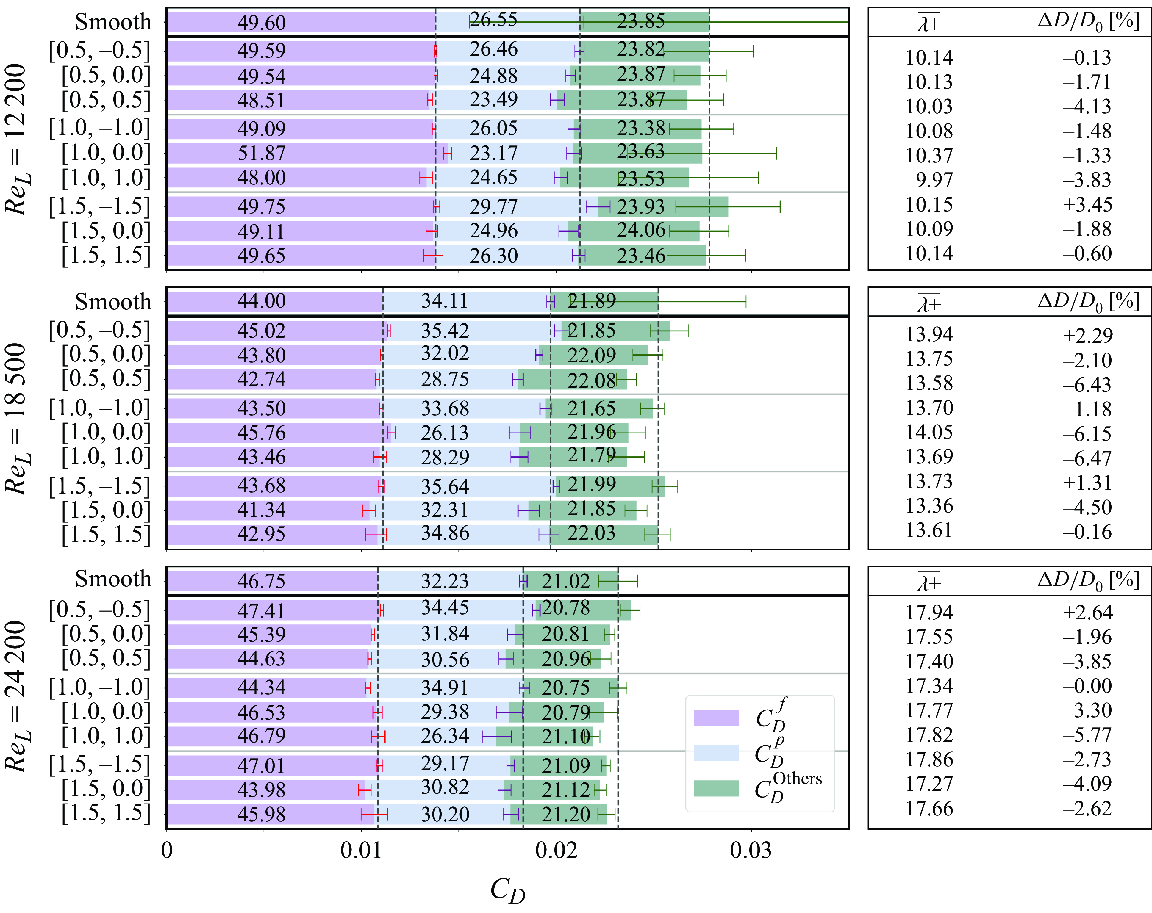
Figure 4. Decomposition of the total drag force, in terms of the drag coefficient, into friction, $C_D^{f}$
, pressure,
$C_D^{f}$
, pressure, $C_D^{p}$
, and
$C_D^{p}$
, and $C_D^{{Others}}$
components for experiments performed at global Reynolds numbers (a)
$C_D^{{Others}}$
components for experiments performed at global Reynolds numbers (a) $\textit{Re}_{L} = 12\,200$
, (b)
$\textit{Re}_{L} = 12\,200$
, (b) $\textit{Re}_{L} = 18\,500$
and (c)
$\textit{Re}_{L} = 18\,500$
and (c) $\textit{Re}_{L} = 24\,200$
for all samples. The error bars on the
$\textit{Re}_{L} = 24\,200$
for all samples. The error bars on the $C_D^f$
are calculated using the upper and lower bounds of the integral of the shear stress discussed in more detail in § SI.2. of the supplementary material. The rest of the error bars correspond to the
$C_D^f$
are calculated using the upper and lower bounds of the integral of the shear stress discussed in more detail in § SI.2. of the supplementary material. The rest of the error bars correspond to the $95\, \%$
confidence intervals of the profile and total drag measurements. Values on each barare the percentage of the contribution of each component with respect to the total drag of the smooth reference sample. For example, for the [1.5,1.5] sample, at
$95\, \%$
confidence intervals of the profile and total drag measurements. Values on each barare the percentage of the contribution of each component with respect to the total drag of the smooth reference sample. For example, for the [1.5,1.5] sample, at $\textit{Re}_{L} = 18\,500$
, frictional drag is
$\textit{Re}_{L} = 18\,500$
, frictional drag is $42.95\, \%$
of the total drag of the smooth reference. In this manner, the sum of the values for smooth samples comes to
$42.95\, \%$
of the total drag of the smooth reference. In this manner, the sum of the values for smooth samples comes to $100\, \%$
. Average
$100\, \%$
. Average $\overline {\lambda ^{+}}$
and the percentage of total drag reduction (sum of the values on each horizontal line minus 100) for all the samples are listed in the table on the right.
$\overline {\lambda ^{+}}$
and the percentage of total drag reduction (sum of the values on each horizontal line minus 100) for all the samples are listed in the table on the right.
As seen in figure 4, within families of ${\mathcal {R}} = 0.5$
and
${\mathcal {R}} = 0.5$
and ${\mathcal {R}} = 1.0$
, concave textures with
${\mathcal {R}} = 1.0$
, concave textures with $\kappa = {\mathcal {R}}$
exhibit the lowest drag force compared with the rest of the samples and convex ones with
$\kappa = {\mathcal {R}}$
exhibit the lowest drag force compared with the rest of the samples and convex ones with $\kappa = -{\mathcal {R}}$
the largest drag. Triangular textures with
$\kappa = -{\mathcal {R}}$
the largest drag. Triangular textures with $\kappa = 0$
show drag values in between that of the
$\kappa = 0$
show drag values in between that of the $\kappa = \pm {\mathcal {R}}$
cases, sometimes close to one or the other depending on the case. However, going to the sharper textures of
$\kappa = \pm {\mathcal {R}}$
cases, sometimes close to one or the other depending on the case. However, going to the sharper textures of ${\mathcal {R}} = 1.5$
, at all Reynolds numbers, sample [1.5, 0.0] (triangular) retains the lowest drag, with the concave [1.5, 1.5] riblet in second place and convex [1.5, –1.5] seeing the largest drag for
${\mathcal {R}} = 1.5$
, at all Reynolds numbers, sample [1.5, 0.0] (triangular) retains the lowest drag, with the concave [1.5, 1.5] riblet in second place and convex [1.5, –1.5] seeing the largest drag for $\textit{Re}_{L} = 12\,200$
and
$\textit{Re}_{L} = 12\,200$
and $18\,500$
. At
$18\,500$
. At $\textit{Re}_{L} = 24\,200$
the concave and convex samples, [1.5, 1.5] and [1.5, –1.5], experience nearly similar values of drag.
$\textit{Re}_{L} = 24\,200$
the concave and convex samples, [1.5, 1.5] and [1.5, –1.5], experience nearly similar values of drag.
While different from BL past foils, this trend seen in the drag as a function of the $\kappa _2$
is similar to the pattern previously reported in the Couette flow and early Taylor vortex regime in a Taylor–Couette flow (Raayai-Ardakani Reference Raayai-Ardakani2022). For shallow textures with
$\kappa _2$
is similar to the pattern previously reported in the Couette flow and early Taylor vortex regime in a Taylor–Couette flow (Raayai-Ardakani Reference Raayai-Ardakani2022). For shallow textures with ${\mathcal {R}} \leqslant 1$
, torque of the riblet-covered rotors decreases as
${\mathcal {R}} \leqslant 1$
, torque of the riblet-covered rotors decreases as $\kappa _2$
is increased (at a constant
$\kappa _2$
is increased (at a constant ${\mathcal {R}}$
). Going to sharper textures such as
${\mathcal {R}}$
). Going to sharper textures such as $\kappa _2 = 1.5$
, the torque does not monotonically follow the
$\kappa _2 = 1.5$
, the torque does not monotonically follow the $\kappa _2$
parameter and the lowest recorded torque is around
$\kappa _2$
parameter and the lowest recorded torque is around $0 \leqslant \kappa _2 \leqslant 0.5$
for riblets with a spacing of 1 mm (spacing normalised by the gap of the Taylor–Couette cell of 0.13). In addition, previous experiments by Walsh & Lindemann (Reference Walsh and Lindemann1984) show larger drag reductions for concave-up semi-circular riblets compared with triangular textures and nearly no drag reduction for convex-up semi-circular riblets. They also show that an increase in the radius of curvature at the trough of triangular textures can reduce the drag while an increase in the radius of curvature at the peak of the grooves slowly increases the drag experienced by the riblets.
$0 \leqslant \kappa _2 \leqslant 0.5$
for riblets with a spacing of 1 mm (spacing normalised by the gap of the Taylor–Couette cell of 0.13). In addition, previous experiments by Walsh & Lindemann (Reference Walsh and Lindemann1984) show larger drag reductions for concave-up semi-circular riblets compared with triangular textures and nearly no drag reduction for convex-up semi-circular riblets. They also show that an increase in the radius of curvature at the trough of triangular textures can reduce the drag while an increase in the radius of curvature at the peak of the grooves slowly increases the drag experienced by the riblets.
In comparison to the smooth reference, the majority of the cases tested here show some level of drag reduction. For the ${\mathcal {R}} = 0.5$
family, only the [0.5, 0.5] and [0.5, 0.0] samples were drag-reducing in all cases. In the
${\mathcal {R}} = 0.5$
family, only the [0.5, 0.5] and [0.5, 0.0] samples were drag-reducing in all cases. In the ${\mathcal {R}} = 1.0$
family, the [1.0, 1.0] sample experiences the largest drag reduction among the rest of the family, with [1.0, 0.0] seeing slightly lower reductions, and the [1.0, –1.0] samples experiencing no reduction at
${\mathcal {R}} = 1.0$
family, the [1.0, 1.0] sample experiences the largest drag reduction among the rest of the family, with [1.0, 0.0] seeing slightly lower reductions, and the [1.0, –1.0] samples experiencing no reduction at $\textit{Re}_{L} = 24\,200$
or reductions of slightly larger than
$\textit{Re}_{L} = 24\,200$
or reductions of slightly larger than $1\,\%$
for the lower Reynolds numbers. For the
$1\,\%$
for the lower Reynolds numbers. For the ${\mathcal {R}} = 1.5$
family, the [1.5, 0.0] sample is able to stay drag-reducing for all the tested Reynolds numbers, while for
${\mathcal {R}} = 1.5$
family, the [1.5, 0.0] sample is able to stay drag-reducing for all the tested Reynolds numbers, while for $\textit{Re}_{L} = 12\,200$
and
$\textit{Re}_{L} = 12\,200$
and $18\,500$
, the [1.5, –1.5]sample is fully drag-increasing and [1.5, 1.5] stays nearly neutral. At the largest Reynolds number of 24 200, all
$18\,500$
, the [1.5, –1.5]sample is fully drag-increasing and [1.5, 1.5] stays nearly neutral. At the largest Reynolds number of 24 200, all ${\mathcal {R}} = 1.5$
samples become drag-reducing.
${\mathcal {R}} = 1.5$
samples become drag-reducing.
Breaking down the measured drag into components, we see that the friction and the pressure drags do not follow the same trend as that of the total drag. Except for a few of the cases reported, the total frictional component of the drag force only experiences marginal changes due to the presence of the textures as discussed more in § 3.2. However, we record substantial levels of reductions in the pressure drag for quite a number of the samples that help in reducing the drag even when the frictional drag is unchanged. While the effect of riblets in changing the pressure distribution and pressure drag has largely been unexplored, recent numerical simulations of riblet-covered bodies (Mele et al. Reference Mele, Tognaccini and Catalano2016, Reference Mele, Tognaccini, Catalano and de Rosa2020; Cacciatori et al. Reference Cacciatori, Brignoli, Mele, Gattere, Monti and Quadrio2022), as well as other skin-friction reduction techniques (Banchetti et al. Reference Banchetti, Luchini and Quadrio2020; Nguyen et al. Reference Nguyen, Ricco and Pironti2021; Quadrio et al. Reference Quadrio, Chiarini, Banchetti, Gatti, Memmolo and Pirozzoli2022) have also confirmed the ability of these techniques to impact the pressure drag as discussed later in § 3.5.
At the lowest Reynolds number, $\textit{Re}_{L} = 12\,200$
, and among the family of
$\textit{Re}_{L} = 12\,200$
, and among the family of ${\mathcal {R}} = 0.5$
, only the
${\mathcal {R}} = 0.5$
, only the $D_{f}$
of the [0.5, 0.5] sample experiences a reduction of
$D_{f}$
of the [0.5, 0.5] sample experiences a reduction of $2.2\, \%$
compared with the smooth reference, contributing
$2.2\, \%$
compared with the smooth reference, contributing $1\, \%$
to the total of
$1\, \%$
to the total of $4.1\, \%$
reduction in the total drag. (Note that the values on each of the bars in figure 4 corresponds to the percentage of the contribution of the specific component with respect to the smooth reference sample at the given Reynolds number.) Among the
$4.1\, \%$
reduction in the total drag. (Note that the values on each of the bars in figure 4 corresponds to the percentage of the contribution of the specific component with respect to the smooth reference sample at the given Reynolds number.) Among the ${\mathcal {R}} = 1.0$
family, both the [1.0, –1.0] and [1.0, 1.0] samples experience
${\mathcal {R}} = 1.0$
family, both the [1.0, –1.0] and [1.0, 1.0] samples experience $1\, \%$
and
$1\, \%$
and $3.2\, \%$
reduction in the
$3.2\, \%$
reduction in the $D_{f}$
, contributing to
$D_{f}$
, contributing to $0.5\, \%$
(out of
$0.5\, \%$
(out of $1.48\, \%$
) and
$1.48\, \%$
) and $1.6\, \%$
(out of the
$1.6\, \%$
(out of the $3.82\, \%$
) to the total drag reductions of these samples, respectively. The [1.0, 0.0] sample on the other hand experiences a
$3.82\, \%$
) to the total drag reductions of these samples, respectively. The [1.0, 0.0] sample on the other hand experiences a $4.6\, \%$
increase in the frictional drag, requiring the pressure drag to contribute a
$4.6\, \%$
increase in the frictional drag, requiring the pressure drag to contribute a $3.6\, \%$
reduction to overcome the added
$3.6\, \%$
reduction to overcome the added $2.27\, \%$
for the sample to experience a
$2.27\, \%$
for the sample to experience a $1.33\, \%$
reduction in the total drag. Similar trends can be extracted for the samples at larger Reynolds numbers (see figure 4).
$1.33\, \%$
reduction in the total drag. Similar trends can be extracted for the samples at larger Reynolds numbers (see figure 4).
Overall, $C_D^{f}$
of
$C_D^{f}$
of ${\mathcal {R}} = 0.5$
and
${\mathcal {R}} = 0.5$
and ${\mathcal {R}} = 1.5$
follows a similar trend as that of the total drag force, while for the
${\mathcal {R}} = 1.5$
follows a similar trend as that of the total drag force, while for the ${\mathcal {R}} = 1.0$
family, unlike the total drag, the trend in
${\mathcal {R}} = 1.0$
family, unlike the total drag, the trend in $C_D^{f}$
is non-monotonic with respect to
$C_D^{f}$
is non-monotonic with respect to $\kappa _2$
, with the [1.0, 1.0] sample experiencing the lowest and [1.0, 0.0] experiencing the highest
$\kappa _2$
, with the [1.0, 1.0] sample experiencing the lowest and [1.0, 0.0] experiencing the highest $C_D^{f}$
at
$C_D^{f}$
at $\textit{Re}_{L} = 12\,200$
and
$\textit{Re}_{L} = 12\,200$
and $18\,500$
, and at the largest
$18\,500$
, and at the largest $\textit{Re}_{L} = 24\,200$
, the [1.0, 1.0] and [1.0, 0.0] samples have nearly similar values of
$\textit{Re}_{L} = 24\,200$
, the [1.0, 1.0] and [1.0, 0.0] samples have nearly similar values of $C_D^{f}$
, which is larger than that of the [1.0, –1.0] sample. Among the
$C_D^{f}$
, which is larger than that of the [1.0, –1.0] sample. Among the ${\mathcal {R}}= 0.5$
case, the magnitude of the pressure drag also takes a decreasing trend with the
${\mathcal {R}}= 0.5$
case, the magnitude of the pressure drag also takes a decreasing trend with the $\kappa _2$
parameter, with [0.5, 0.5] experiencing the lowest
$\kappa _2$
parameter, with [0.5, 0.5] experiencing the lowest $C_D^{p}$
and [0.5, –0.5] experiencing the largest one. As a results, [0.5, 0.5] and [0.5, 0.0] also experience a reduction in
$C_D^{p}$
and [0.5, –0.5] experiencing the largest one. As a results, [0.5, 0.5] and [0.5, 0.0] also experience a reduction in $C_D^{p}$
compared with the smooth sample while [0.5, −0.5] stays either neutral or
$C_D^{p}$
compared with the smooth sample while [0.5, −0.5] stays either neutral or $C_D^{p}$
-increasing. Thus, within this family, cumulatively with
$C_D^{p}$
-increasing. Thus, within this family, cumulatively with $C_D^{f}$
, only the [0.5, 0.0] and [0.5, 0.5] samples are drag-reducing. Among the
$C_D^{f}$
, only the [0.5, 0.0] and [0.5, 0.5] samples are drag-reducing. Among the ${\mathcal {R}} = 1.0$
family, at
${\mathcal {R}} = 1.0$
family, at $\textit{Re}_{L} = 12\,200$
and
$\textit{Re}_{L} = 12\,200$
and $18\,500$
, the [1.0, 0.0] sample experiences the lowest
$18\,500$
, the [1.0, 0.0] sample experiences the lowest $C_D^{p}$
, while at
$C_D^{p}$
, while at $\textit{Re}_{L} = 24\,200$
the [1.0, 1.0] sample has the lowest
$\textit{Re}_{L} = 24\,200$
the [1.0, 1.0] sample has the lowest $C_D^{p}$
and the [1.0, –1.0] sample experiences the largest
$C_D^{p}$
and the [1.0, –1.0] sample experiences the largest $C_D^{p}$
among them all. The [1.0, 0.0] sample, which could not offer any frictional reduction, experiences a large enough reduction in the pressure drag to be cumulatively drag-reducing. Similarly, for the [1.0, 1.0] sample, the reduction achievable in the pressure drag enhances the cumulative drag reduction of this sample. For the [1.0, –1.0] sample, the pressure drag is not able to enhance the drag reduction at
$C_D^{p}$
among them all. The [1.0, 0.0] sample, which could not offer any frictional reduction, experiences a large enough reduction in the pressure drag to be cumulatively drag-reducing. Similarly, for the [1.0, 1.0] sample, the reduction achievable in the pressure drag enhances the cumulative drag reduction of this sample. For the [1.0, –1.0] sample, the pressure drag is not able to enhance the drag reduction at $\textit{Re}_{L} = 12\,200$
and
$\textit{Re}_{L} = 12\,200$
and $18\,500$
, and at
$18\,500$
, and at $\textit{Re}_{L} = 24\,200$
it even diminishes the drag reduction that was achieved from the frictional component. For the sharpest riblet family, at
$\textit{Re}_{L} = 24\,200$
it even diminishes the drag reduction that was achieved from the frictional component. For the sharpest riblet family, at $\textit{Re}_{L} = 12\,200$
and
$\textit{Re}_{L} = 12\,200$
and $18\,500$
, [1.5, 0.0] experiences the lowest pressure drag and [1.5, –1.5] the largest, and only [1.5, 0.0] is able to see a cumulative reduction in the drag force. At
$18\,500$
, [1.5, 0.0] experiences the lowest pressure drag and [1.5, –1.5] the largest, and only [1.5, 0.0] is able to see a cumulative reduction in the drag force. At $\textit{Re}_{L} = 24\,200$
, the pressure drag experienced by the three samples is nearly similar and all three are able to capture a reduction in the pressure drag, which also leads to them being cumulatively drag-reducing as well.
$\textit{Re}_{L} = 24\,200$
, the pressure drag experienced by the three samples is nearly similar and all three are able to capture a reduction in the pressure drag, which also leads to them being cumulatively drag-reducing as well.
While the foils used here operate in the laminar regime and have a lower $\textit{Re}_{L}$
compared with the
$\textit{Re}_{L}$
compared with the $\textit{Re}_c$
of the previously reported cases with riblets used on airfoils, we use an average wall shear stress based on the total frictional drag force to find an average
$\textit{Re}_c$
of the previously reported cases with riblets used on airfoils, we use an average wall shear stress based on the total frictional drag force to find an average $\overline {\lambda ^{+}}$
for the entirety of the samples as reported in figure 4. Recognising the difference in the flow fields, we can still attempt to compare the results against the previous reports, especially for the case of the triangular riblets with
$\overline {\lambda ^{+}}$
for the entirety of the samples as reported in figure 4. Recognising the difference in the flow fields, we can still attempt to compare the results against the previous reports, especially for the case of the triangular riblets with $\kappa _2 = 0$
. Coustols (Reference Coustols1989) reports a
$\kappa _2 = 0$
. Coustols (Reference Coustols1989) reports a $2.7\, \%$
reduction for
$2.7\, \%$
reduction for $\lambda ^{+}=10$
, while Subashchandar et al. (Reference Subashchandar, Rajeev and Sundaram1995) and Subaschandar et al. (Reference Subaschandar, Kumar and Sundaram1999) report a
$\lambda ^{+}=10$
, while Subashchandar et al. (Reference Subashchandar, Rajeev and Sundaram1995) and Subaschandar et al. (Reference Subaschandar, Kumar and Sundaram1999) report a $15\, \%$
reduction and Caram & Ahmed (Reference Caram and Ahmed1991) report a
$15\, \%$
reduction and Caram & Ahmed (Reference Caram and Ahmed1991) report a $13.3\, \%$
reduction. For
$13.3\, \%$
reduction. For $10\lt \lambda ^{+}\lt 15$
, Sundaram et al. (Reference Sundaram, Viswanath and Rudrakumar1996) report a
$10\lt \lambda ^{+}\lt 15$
, Sundaram et al. (Reference Sundaram, Viswanath and Rudrakumar1996) report a $16\, \%$
reduction. For all these cases, the height and spacing of the grooves are the same and, thus,
$16\, \%$
reduction. For all these cases, the height and spacing of the grooves are the same and, thus, $A^{+} = \lambda ^{+}$
. Chamorro et al. (Reference Chamorro, Arndt and Sotiropoulos2013) report a max imumreduction of
$A^{+} = \lambda ^{+}$
. Chamorro et al. (Reference Chamorro, Arndt and Sotiropoulos2013) report a max imumreduction of $5\, \%$
for
$5\, \%$
for $\lambda ^{+} \approx 11{-}14$
. In the cases reported here, the closest situation is the sharpest riblet of
$\lambda ^{+} \approx 11{-}14$
. In the cases reported here, the closest situation is the sharpest riblet of ${\mathcal {R}} = 1.5$
where, for
${\mathcal {R}} = 1.5$
where, for $\lambda ^{+} \approx 10$
, the reductions achieved are around
$\lambda ^{+} \approx 10$
, the reductions achieved are around $1.88\, \%$
, increasing to
$1.88\, \%$
, increasing to $4.5\, \%$
for
$4.5\, \%$
for ${\lambda ^{+}} = 13.36$
and reducing to
${\lambda ^{+}} = 13.36$
and reducing to $4.09\, \%$
for
$4.09\, \%$
for $\lambda ^{+} = 17.27$
. Since the previously reported cases are all for
$\lambda ^{+} = 17.27$
. Since the previously reported cases are all for $\textit{Re}_c\gt 10^5$
, one could hypothesise that the larger reductions reported can potentially be related to reductions in the Reynolds shear stresses close to the wall that are absent in the current results.
$\textit{Re}_c\gt 10^5$
, one could hypothesise that the larger reductions reported can potentially be related to reductions in the Reynolds shear stresses close to the wall that are absent in the current results.
Lastly, as can be seen from the percentages listed on the bars of figure 4, the contributions attributed to the $D_{{others}}$
, not captured via the PIV measurements, do not show any clear dependence on the textures and have nearly similar values and so are not discussed further. We believe this component is mainly due the three-dimensional edge effects of the low-aspect ratio foils used in the study as well as the impact of a shield (see figure 3) used to reduce the effect of the flow on the strut connecting the sample to the linear variable differential transformer sensor.
$D_{{others}}$
, not captured via the PIV measurements, do not show any clear dependence on the textures and have nearly similar values and so are not discussed further. We believe this component is mainly due the three-dimensional edge effects of the low-aspect ratio foils used in the study as well as the impact of a shield (see figure 3) used to reduce the effect of the flow on the strut connecting the sample to the linear variable differential transformer sensor.
3.2. Friction drag
Out of the total drag force exerted on the slender samples, between $40\, \%\!-\!50\,\%$
of the drag is due to the frictional component,
$40\, \%\!-\!50\,\%$
of the drag is due to the frictional component, $D_{f}$
(as seen from the values written on purple portions of the bar plots in figure 4). This component is comprised of the frictional drag experienced on either side of the sample found using the integral of the spanwise-averaged shear stress distributions as
$D_{f}$
(as seen from the values written on purple portions of the bar plots in figure 4). This component is comprised of the frictional drag experienced on either side of the sample found using the integral of the spanwise-averaged shear stress distributions as
 \begin{align} D_{f} = D_{\textit{Front}} + D_{\textit{Back}} = b\left ({\int _0^{L}} \langle {\tau _{n=0}} \rangle _{\textit{Front}}\, {\textrm {d}}x + {\int _0^{L}} \langle {\tau_{n=0}} \rangle _{\textit{Back}}\, {\textrm {d}}x \right). \end{align}
It should be noted that we use the control volume analysis inside the groove as discussed in § SI.2 of the supplementary material to calculate the upper and lower bounds of the difference between the $\langle \tau _{n=0} \rangle$
and
$\langle \tau _{n=0} \rangle$
and $\langle \tau _{{ w}} \rangle$
(where
$\langle \tau _{{ w}} \rangle$
(where $\langle \tau _{{ w}} \rangle$
is the spanwise-averaged shear stress distribution on the riblet wall) and use them in the integral of (3.1) and present them as the errorbars shown on the
$\langle \tau _{{ w}} \rangle$
is the spanwise-averaged shear stress distribution on the riblet wall) and use them in the integral of (3.1) and present them as the errorbars shown on the $D_f$
in figure 4. Along each side, (3.1) can be divided into the contributions of the LE, LET and Flat region as written in the form of
$D_f$
in figure 4. Along each side, (3.1) can be divided into the contributions of the LE, LET and Flat region as written in the form of
 \begin{align} D_{\textit{Front}} = b \left ({\int _0^{x_{\textit{LET}}}} \langle {\tau _{n=0}} \rangle _{\textit{Front}} (x) {\textrm {d}}x + {\int _{x_{\textit{LET}}}^{x_{\textit{Flat}}}} \langle {\tau _{n=0}} \rangle _{\textit{Front}} \,(x) {\textrm {d}}x + {\int _{x_{\textit{Flat}}}^{L}} \langle {\tau _{n=0}} \rangle _{\textit{Front}} \, (x) {\textrm {d}}x \right ) \end{align}
and $D_{Back} = {D_{Back}^{LE}} + {D_{Back}^{LET}} + {D_{Back}^{Flat}}$
. Note that the spanwise-averaged wall shear stress distribution,
$D_{Back} = {D_{Back}^{LE}} + {D_{Back}^{LET}} + {D_{Back}^{Flat}}$
. Note that the spanwise-averaged wall shear stress distribution, $\langle {\tau _{n=0}} \rangle$
, is the shear stress component exerted along the surface, or
$\langle {\tau _{n=0}} \rangle$
, is the shear stress component exerted along the surface, or $\hat {s}$
, with
$\hat {s}$
, with $\theta$
the local angle between the
$\theta$
the local angle between the $x$
and
$x$
and $\hat {s}$
directions. Thus, with
$\hat {s}$
directions. Thus, with ${\textrm {d}}x = \cos \theta {\textrm {d}}s$
, we have
${\textrm {d}}x = \cos \theta {\textrm {d}}s$
, we have $\langle {\tau _{n=0}} \rangle \cos \theta {\textrm {d}}s = \langle {\tau _{n=0}} \rangle {\textrm {d}}x$
.
$\langle {\tau _{n=0}} \rangle \cos \theta {\textrm {d}}s = \langle {\tau _{n=0}} \rangle {\textrm {d}}x$
.
In addition to the cumulative form of the $D_{f}$
shown in figure 4 (purple bars), the contributions of each side of the sample, as well as the LE, LET and Flat segments on
$D_{f}$
shown in figure 4 (purple bars), the contributions of each side of the sample, as well as the LE, LET and Flat segments on $D_{f}$
are presented in figure 5. Firstly, due to the small angle of attack, the contribution of the pressure side is larger than the suction side for all the samples, including the smooth reference. In addition, for all the riblet samples except for [0.5, 0.5] at
$D_{f}$
are presented in figure 5. Firstly, due to the small angle of attack, the contribution of the pressure side is larger than the suction side for all the samples, including the smooth reference. In addition, for all the riblet samples except for [0.5, 0.5] at $\textit{Re}_{L} = 18\,500$
and
$\textit{Re}_{L} = 18\,500$
and $24\,200$
, and [1.0, –1.0] and [1.5, 0.0] at
$24\,200$
, and [1.0, –1.0] and [1.5, 0.0] at $\textit{Re}_{L} = 24\,200$
, the pressure sides experience drag increases compared with the smooth reference, and reduction in frictional drag is mostly visible on the suction sides. All members of the
$\textit{Re}_{L} = 24\,200$
, the pressure sides experience drag increases compared with the smooth reference, and reduction in frictional drag is mostly visible on the suction sides. All members of the ${\mathcal {R}} = 1.5$
family experience a reduction in the frictional drag on the suction side. Among the other families, [0.5, –0.5] becomes
${\mathcal {R}} = 1.5$
family experience a reduction in the frictional drag on the suction side. Among the other families, [0.5, –0.5] becomes $D_{f}$
-increasing at
$D_{f}$
-increasing at $\textit{Re}_{L} = 18\,500$
and
$\textit{Re}_{L} = 18\,500$
and $24\,200$
andthe [1.0, 0.0] sample is either neutral or
$24\,200$
andthe [1.0, 0.0] sample is either neutral or $D_{f}$
-increasing at
$D_{f}$
-increasing at $\textit{Re}_{L} = 12\,200$
and
$\textit{Re}_{L} = 12\,200$
and $18\,500$
, while the rest of the cases remain
$18\,500$
, while the rest of the cases remain $D_{f}$
-decreasing.
$D_{f}$
-decreasing.
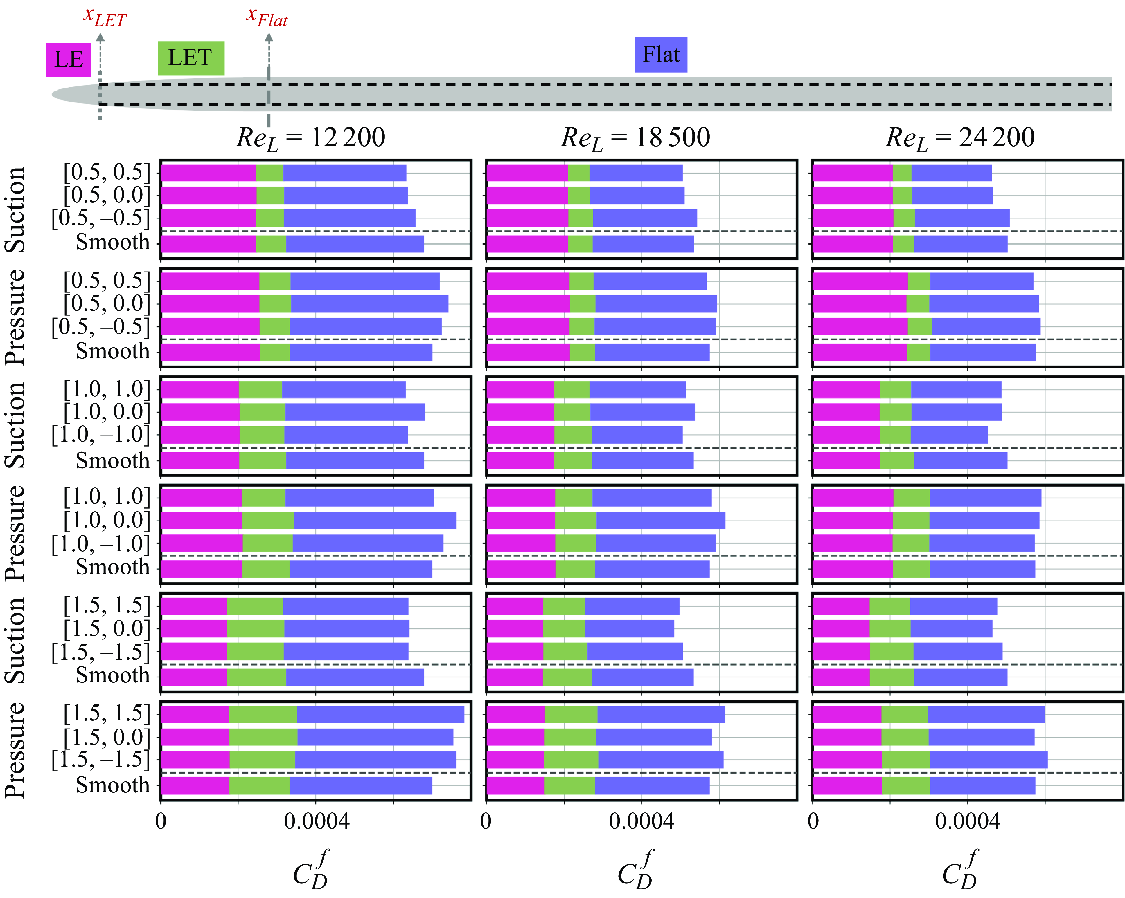
Figure 5. Bar plots showing the contributions of LE, LET and Flat regions on either side of the riblet samples to the frictional drag coefficient. Locations of $x_{{ LET}}$
and
$x_{{ LET}}$
and $x_{{ Flat}}$
are shown on the top schematic, corresponding to the bounds in the integrals of (3.2).
$x_{{ Flat}}$
are shown on the top schematic, corresponding to the bounds in the integrals of (3.2).
The LE region captures $14\, \%$
,
$14\, \%$
, $10\, \%$
and
$10\, \%$
and $7.5\, \%$
of the length of
$7.5\, \%$
of the length of ${\mathcal {R}} = 0.5$
,
${\mathcal {R}} = 0.5$
, ${\mathcal {R}} = 1.0$
and
${\mathcal {R}} = 1.0$
and ${\mathcal {R}} = 1.5$
families, respectively. The LE region experiences the largest levels of local shear stress as is expected from a developing BL. Without any riblets in this area, the drag experienced by the LE regions (dark magenta bars in figure 5) of all samples of the constant-
${\mathcal {R}} = 1.5$
families, respectively. The LE region experiences the largest levels of local shear stress as is expected from a developing BL. Without any riblets in this area, the drag experienced by the LE regions (dark magenta bars in figure 5) of all samples of the constant- ${\mathcal {R}}$
family experience nearly the same levels of
${\mathcal {R}}$
family experience nearly the same levels of $D_{f}$
at a constant Reynolds number and, for both sides, the
$D_{f}$
at a constant Reynolds number and, for both sides, the $C_D^{{ LE}}$
are within
$C_D^{{ LE}}$
are within $0.1\, \%$
of the contributions found for the smooth surface (
$0.1\, \%$
of the contributions found for the smooth surface ( $C_{D,0}^{{ LE}}$
). Thus, the LE regions do not contribute to the drag change and this portion of the frictional drag,
$C_{D,0}^{{ LE}}$
). Thus, the LE regions do not contribute to the drag change and this portion of the frictional drag, $C_D^{{ LE}}$
, is not available for modification by the riblets. With the difference in the starting point of the riblets, i.e.
$C_D^{{ LE}}$
, is not available for modification by the riblets. With the difference in the starting point of the riblets, i.e. $x_{{ LET}}$
, for the different families, the
$x_{{ LET}}$
, for the different families, the ${\mathcal {R}} = 0.5$
family experiences the largest contribution from the
${\mathcal {R}} = 0.5$
family experiences the largest contribution from the $C_D^{{ LE}}$
region, with
$C_D^{{ LE}}$
region, with ${\mathcal {R}} = 1.0$
getting a lower contribution, and
${\mathcal {R}} = 1.0$
getting a lower contribution, and ${\mathcal {R}} = 1.50$
capturing the lowest contribution from the LE region.
${\mathcal {R}} = 1.50$
capturing the lowest contribution from the LE region.
Based on $x_{{ LET}}$
,
$x_{{ LET}}$
, $11\, \%$
,
$11\, \%$
, $15\, \%$
and
$15\, \%$
and $17.5\, \%$
of the length of the
$17.5\, \%$
of the length of the ${\mathcal {R}} = 0.5$
,
${\mathcal {R}} = 0.5$
, ${\mathcal {R}} = 1.0$
and
${\mathcal {R}} = 1.0$
and ${\mathcal {R}} = 1.5$
samples is comprised of the growing riblets in the LET region, respectively. Thus, as shown in figure 5, in reverse order compared with the LE regions, the LET portion of the
${\mathcal {R}} = 1.5$
samples is comprised of the growing riblets in the LET region, respectively. Thus, as shown in figure 5, in reverse order compared with the LE regions, the LET portion of the ${\mathcal {R}} = 1.5$
family captures a larger portion of the total
${\mathcal {R}} = 1.5$
family captures a larger portion of the total $D_{f}$
on either side of the sample, compared with
$D_{f}$
on either side of the sample, compared with ${\mathcal {R}} = 1.0$
, and
${\mathcal {R}} = 1.0$
, and ${\mathcal {R}} = 1.0$
has a larger
${\mathcal {R}} = 1.0$
has a larger $C_D^{\textit{LET}}$
than the
$C_D^{\textit{LET}}$
than the ${\mathcal {R}} = 0.5$
family. With the BL still developing in this region, the magnitudes of the local
${\mathcal {R}} = 0.5$
family. With the BL still developing in this region, the magnitudes of the local $\langle \tau _{n=0} \rangle$
are still large in this segment and while only capturing less than
$\langle \tau _{n=0} \rangle$
are still large in this segment and while only capturing less than $18\, \%$
of the total length,
$18\, \%$
of the total length, $C_D^{\textit{LET}}$
captures a considerable portion of the total drag force on either side, especially for the sharper riblets of the
$C_D^{\textit{LET}}$
captures a considerable portion of the total drag force on either side, especially for the sharper riblets of the ${\mathcal {R}} = 1.5$
and
${\mathcal {R}} = 1.5$
and ${\mathcal {R}} = 1.0$
families. While the changes in the
${\mathcal {R}} = 1.0$
families. While the changes in the $C_D^{\textit{LET}}$
is a small portion of the total change the frictional drag experiences, the changes in this region act as a starting point toward drag-reducing or drag-increasing riblets and will be discussed more in § 3.3. The Flat segment, capturing
$C_D^{\textit{LET}}$
is a small portion of the total change the frictional drag experiences, the changes in this region act as a starting point toward drag-reducing or drag-increasing riblets and will be discussed more in § 3.3. The Flat segment, capturing $75\, \%$
of the length, experiences the largest portion of the
$75\, \%$
of the length, experiences the largest portion of the $C_D^{f}$
.
$C_D^{f}$
.
Cumulatively, the drag on the suction sides of all samples and at all Reynolds numbers follow similar trends with respect to $\kappa _2$
as that of the total
$\kappa _2$
as that of the total $D_{f}$
, as discussed in § 3.1. On the pressure side however, while
$D_{f}$
, as discussed in § 3.1. On the pressure side however, while ${\mathcal {R}} = 1.0$
and
${\mathcal {R}} = 1.0$
and $1.5$
follow the same trend as the total
$1.5$
follow the same trend as the total $D_{f}$
, the frictional drag of the pressure side ofthe
$D_{f}$
, the frictional drag of the pressure side ofthe ${\mathcal {R}} = 0.5$
family is non-monotonic with
${\mathcal {R}} = 0.5$
family is non-monotonic with $\kappa _2$
with the [0.5, 0.0] sample experiencing the largest
$\kappa _2$
with the [0.5, 0.0] sample experiencing the largest $D_{f}^{\textit{Pressure}}$
. Overall, since the total
$D_{f}^{\textit{Pressure}}$
. Overall, since the total $D_f$
is the result of the sum of two integrals, the distribution of the
$D_f$
is the result of the sum of two integrals, the distribution of the $\langle C_{f} \rangle$
on either side of the sample as well as the difference between the
$\langle C_{f} \rangle$
on either side of the sample as well as the difference between the $\langle \tau_{n=0} \rangle$
and the
$\langle \tau_{n=0} \rangle$
and the $\tau _{0}$
of the smooth reference will be the key parameters in characterising the variations discussed in this section.
$\tau _{0}$
of the smooth reference will be the key parameters in characterising the variations discussed in this section.
3.3. Local shear stress distribution
To explain the trend in the friction drag, and its decomposition in terms of the suction/pressure side, as well as the LE, LET and Flat part of the plate, we focus on the local spanwise-averaged skin-friction coefficient distributions, $\langle C_f \rangle (x)$
. In general, we see fourtypes of
$\langle C_f \rangle (x)$
. In general, we see fourtypes of $\langle C_f \rangle (x)$
as a function of the local Reynolds number,
$\langle C_f \rangle (x)$
as a function of the local Reynolds number, $\textit{Re}_x = \rho U(x) x/\mu$
, where
$\textit{Re}_x = \rho U(x) x/\mu$
, where $U(x)$
is the velocity at the edge of the BL and is nearly always larger than
$U(x)$
is the velocity at the edge of the BL and is nearly always larger than $U_{\infty }$
. Overall, these
$U_{\infty }$
. Overall, these $\langle C_f \rangle (x)$
distributions show a more pronounced dependence on the total length of the foil and the location along the plate with respect to that (
$\langle C_f \rangle (x)$
distributions show a more pronounced dependence on the total length of the foil and the location along the plate with respect to that ( $x/L$
). The effect of the global Reynolds number (as dictated by
$x/L$
). The effect of the global Reynolds number (as dictated by $U_{\infty }$
) is more visible in the order of magnitude of the values
$U_{\infty }$
) is more visible in the order of magnitude of the values $\langle C_f \rangle (x)$
.
$\langle C_f \rangle (x)$
.

Figure 6. Four types of shear stress distribution observed in flow over riblets and representative examples from the data. (a) Type I forthe [0.5, –0.5] sample, at $\textit{Re}_{L}= 12\,200$
suction side. (b) Type II for the [0.5, 0.0] sample, at
$\textit{Re}_{L}= 12\,200$
suction side. (b) Type II for the [0.5, 0.0] sample, at ${ Re}_{L}= 18\,500$
pressure side. (c) Type III for the [1.0, 1.0] sample, at
${ Re}_{L}= 18\,500$
pressure side. (c) Type III for the [1.0, 1.0] sample, at ${ Re}_{L}= 12\,200$
suction side. (d) Type IV for the [1.0, 0.0] sample, at
${ Re}_{L}= 12\,200$
suction side. (d) Type IV for the [1.0, 0.0] sample, at ${ Re}_{L}= 18\,500$
suction side. Colours and markers match the colours and markers used in the upcoming plots. Contour plots of (e)
${ Re}_{L}= 18\,500$
suction side. Colours and markers match the colours and markers used in the upcoming plots. Contour plots of (e) $u$
and (f)
$u$
and (f) $v$
for riblet sample [1.0, 1.0] operated at
$v$
for riblet sample [1.0, 1.0] operated at ${ Re}_{L} = 24\,200$
.
${ Re}_{L} = 24\,200$
.
In the first type (type I), shown in figure 6(a), the $\langle C_f \rangle (x)$
first follows a fast decreasing trend (as expected) as a function of the
$\langle C_f \rangle (x)$
first follows a fast decreasing trend (as expected) as a function of the ${ Re}_x$
, starting in the LE, continuing in the LET and up to early in the Flat region. Afterward, the decreasing trend continues but at a much lower rate than in the first segment (lower than the
${ Re}_x$
, starting in the LE, continuing in the LET and up to early in the Flat region. Afterward, the decreasing trend continues but at a much lower rate than in the first segment (lower than the ${ Re}_x^{-1/2}$
of the Blasius BL theory (Schlichting & Gersten Reference Schlichting and Gersten2016)), until close to the trailing edge, where the
${ Re}_x^{-1/2}$
of the Blasius BL theory (Schlichting & Gersten Reference Schlichting and Gersten2016)), until close to the trailing edge, where the $\langle C_f \rangle (x)$
takes an increasing trend with
$\langle C_f \rangle (x)$
takes an increasing trend with ${ Re}_x$
. The smooth sample also follows a type I trend for all the Reynolds numbers and on both the suction and pressure sides (Fu & Raayai-Ardakani Reference Fu and Raayai-Ardakani2023). In the second type (type II), shown in figure 6(b),
${ Re}_x$
. The smooth sample also follows a type I trend for all the Reynolds numbers and on both the suction and pressure sides (Fu & Raayai-Ardakani Reference Fu and Raayai-Ardakani2023). In the second type (type II), shown in figure 6(b), $\langle C_f \rangle (x)$
starts with a decreasing trend throughout LE, LET and early in the Flat region, and then
$\langle C_f \rangle (x)$
starts with a decreasing trend throughout LE, LET and early in the Flat region, and then $\langle C_f \rangle (x)$
becomes nearly constant in the Flat region, until close to the trailing edge,
$\langle C_f \rangle (x)$
becomes nearly constant in the Flat region, until close to the trailing edge, $\langle C_f \rangle (x)$
slightly increases. In the third type (type III), shown in figure 6(c),
$\langle C_f \rangle (x)$
slightly increases. In the third type (type III), shown in figure 6(c), $\langle C_f \rangle (x)$
starts in a similar manner as types I and II, and the difference starts in the second part where after reaching a minimum
$\langle C_f \rangle (x)$
starts in a similar manner as types I and II, and the difference starts in the second part where after reaching a minimum $\langle C_f \rangle$
in the early portion of the Flat region,
$\langle C_f \rangle$
in the early portion of the Flat region, $\langle C_f \rangle (x)$
takes an increasing trend continuing to the trailing edge, with the increase at the trailing edge having a slightly faster rate. In the fourth type (type IV), shown in figure 6(d), in the early portion, the same decreasing trend as that of types I, II and III is visible. However, in this case, the decrease continues to a minimum, followed by an increase, leading to a region with near constant
$\langle C_f \rangle (x)$
takes an increasing trend continuing to the trailing edge, with the increase at the trailing edge having a slightly faster rate. In the fourth type (type IV), shown in figure 6(d), in the early portion, the same decreasing trend as that of types I, II and III is visible. However, in this case, the decrease continues to a minimum, followed by an increase, leading to a region with near constant $\langle C_f \rangle (x)$
or
$\langle C_f \rangle (x)$
or $\langle C_f \rangle (x)$
-increasing at a very low rate of change, before getting close to the trailing edge where the
$\langle C_f \rangle (x)$
-increasing at a very low rate of change, before getting close to the trailing edge where the $\langle C_f \rangle (x)$
increases at a faster rate.
$\langle C_f \rangle (x)$
increases at a faster rate.
It should be pointed out that in the vicinity of the trailing edge, the $\langle C_f \rangle (x)$
of all samples experiences an increasing trend, different from that usually expected from the BL. This is due to the finite thickness of the sample and how toward the trailing edge while
$\langle C_f \rangle (x)$
of all samples experiences an increasing trend, different from that usually expected from the BL. This is due to the finite thickness of the sample and how toward the trailing edge while $u$
maintains a familiar behaviour (figure 6
e), the velocity in the
$u$
maintains a familiar behaviour (figure 6
e), the velocity in the $y$
direction,
$y$
direction, $v$
(figure 6
f), changes sign compared with earlier along the plate, moving toward the body and not away from the surface. In a developing BL, as seen in the earlier portion of the plate,
$v$
(figure 6
f), changes sign compared with earlier along the plate, moving toward the body and not away from the surface. In a developing BL, as seen in the earlier portion of the plate, $v$
is always away from the surface (see the colour contours of figure 6
f), but from
$v$
is always away from the surface (see the colour contours of figure 6
f), but from $x/L \approx 0.7$
,
$x/L \approx 0.7$
, $v$
changes direction toward the plane (change in the colour contours) and, as a result, the velocity profiles are pushed into the surface resulting in a more attached BL and, thus, increase in
$v$
changes direction toward the plane (change in the colour contours) and, as a result, the velocity profiles are pushed into the surface resulting in a more attached BL and, thus, increase in $\langle C_f \rangle (x)$
for both smooth (Fu & Raayai-Ardakani Reference Fu and Raayai-Ardakani2023) and riblet samples. This trend has been reported in second-order models of a BL over finite-length plates as well(Dennis Reference Dennis1985).
$\langle C_f \rangle (x)$
for both smooth (Fu & Raayai-Ardakani Reference Fu and Raayai-Ardakani2023) and riblet samples. This trend has been reported in second-order models of a BL over finite-length plates as well(Dennis Reference Dennis1985).
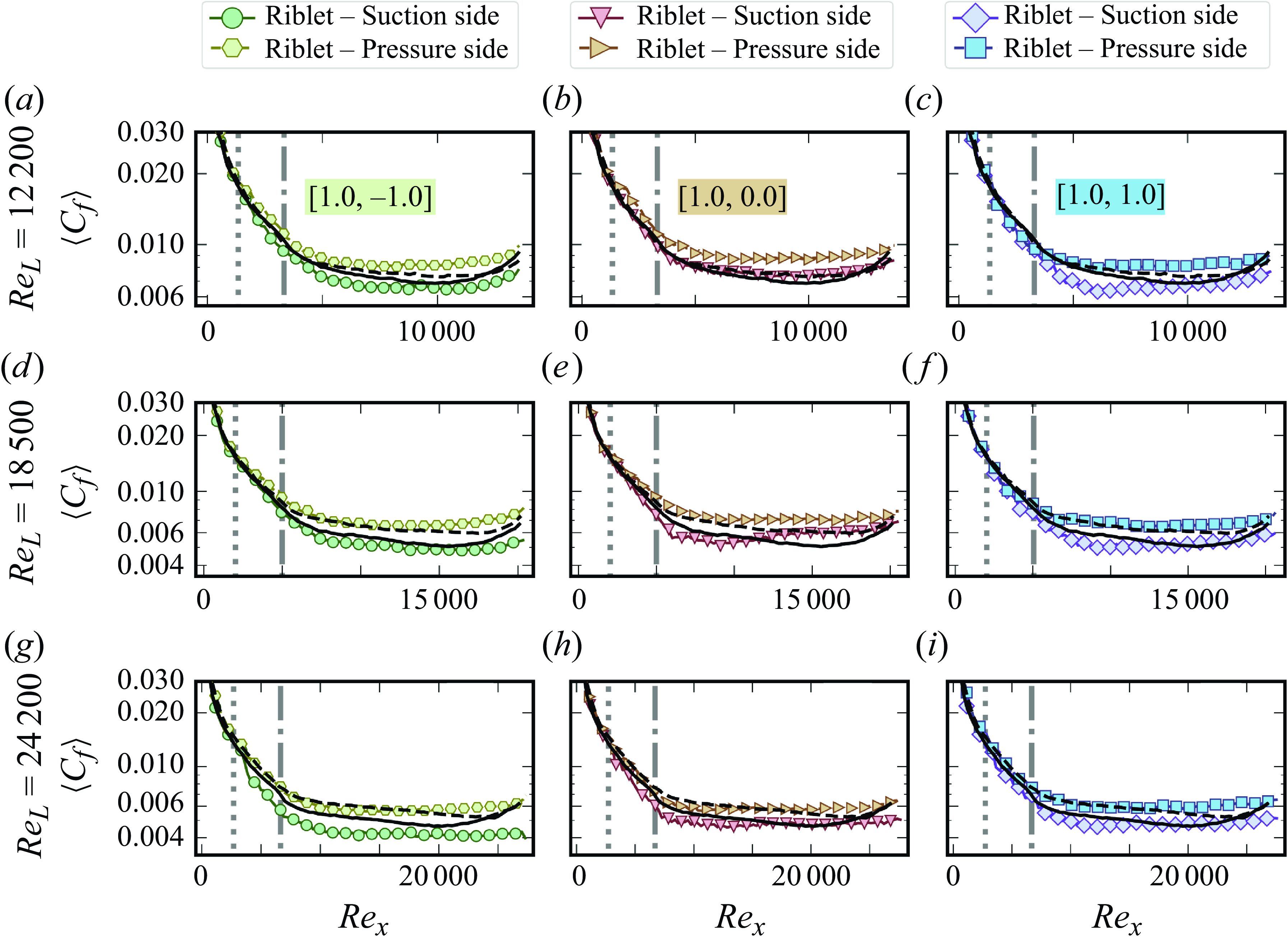
Figure 7. Distribution of $\langle C_f \rangle (x)$
for all the riblet samples of
$\langle C_f \rangle (x)$
for all the riblet samples of ${\mathcal {R}} = 1.0$
for all the Reynolds numbers. The
${\mathcal {R}} = 1.0$
for all the Reynolds numbers. The $C_{f,0}(x)$
of the reference smooth sample on the suction and pressure side are shown with solid and dashed black lines, respectively. Locations of
$C_{f,0}(x)$
of the reference smooth sample on the suction and pressure side are shown with solid and dashed black lines, respectively. Locations of $x_{{ LET}}$
and
$x_{{ LET}}$
and $x_{{ Flat}}$
are marked by grey dotted and dash-dotted vertical lines.
$x_{{ Flat}}$
are marked by grey dotted and dash-dotted vertical lines.
The local distributions of $\langle C_f \rangle (x)$
are presented in figures 7 and SI.4(A-C) of the supplementary material for the suction and pressure sides of all the samples and at all global Reynolds numbers, as well as the accompanying distributions of the difference between the spanwise-averaged shear stress of the riblet samples and the smooth reference,
$\langle C_f \rangle (x)$
are presented in figures 7 and SI.4(A-C) of the supplementary material for the suction and pressure sides of all the samples and at all global Reynolds numbers, as well as the accompanying distributions of the difference between the spanwise-averaged shear stress of the riblet samples and the smooth reference, $\unicode{x1D6E5} \langle \tau _{n=0} \rangle$
, normalised locally by that of the smooth reference,
$\unicode{x1D6E5} \langle \tau _{n=0} \rangle$
, normalised locally by that of the smooth reference, $\tau {_0}$
(figure SI.4(D-F)). In addition, a phase map of the type of shear stress distribution as a function of
$\tau {_0}$
(figure SI.4(D-F)). In addition, a phase map of the type of shear stress distribution as a function of ${\mathcal {R}}$
and
${\mathcal {R}}$
and $\kappa _2$
for all the samples and the global Reynolds numbers is shown in figure 8. While the
$\kappa _2$
for all the samples and the global Reynolds numbers is shown in figure 8. While the $\langle C_f \rangle (x)$
distributions follow only four patterns as driven by the BL development along the samples (more details in the upcoming § 3.4), within each type, we see a variety of patterns when considering the corresponding
$\langle C_f \rangle (x)$
distributions follow only four patterns as driven by the BL development along the samples (more details in the upcoming § 3.4), within each type, we see a variety of patterns when considering the corresponding $\unicode{x1D6E5} \langle \tau _{n=0} \rangle /\tau _0$
distribution, as discussed in more detail below.
$\unicode{x1D6E5} \langle \tau _{n=0} \rangle /\tau _0$
distribution, as discussed in more detail below.

Figure 8. Phase map summarising the type of distribution of the $\langle C_f \rangle (x)$
as a function of
$\langle C_f \rangle (x)$
as a function of ${\mathcal {R}}$
and
${\mathcal {R}}$
and $\kappa _2$
for the suction and pressure sides and the global Reynolds numbers. Signs (–/+) on the top right -handside of the markers indicate the drag-reducing/increasing nature of those sides of the samples (frictional component).
$\kappa _2$
for the suction and pressure sides and the global Reynolds numbers. Signs (–/+) on the top right -handside of the markers indicate the drag-reducing/increasing nature of those sides of the samples (frictional component).
For all the cases, prior to the start of the textures, in the LE region the plates experience $\langle C_f \rangle (x)$
nearly identical to that of the smooth reference plate (
$\langle C_f \rangle (x)$
nearly identical to that of the smooth reference plate ( $C_{f,0}(x)$
) as expected. Hence, we record similar values of
$C_{f,0}(x)$
) as expected. Hence, we record similar values of $C_D^{{ LE}}$
for all the members of each family and the smooth surface as shown in § 3.2. As the riblets start and grow in the LET region, the
$C_D^{{ LE}}$
for all the members of each family and the smooth surface as shown in § 3.2. As the riblets start and grow in the LET region, the $\langle C_f \rangle (x)$
starts to deviate from that of the smooth reference. As discussed earlier in § 2.2, the design of the leading edge mimicking the nose of a shark (Lauder et al. Reference Lauder, Wainwright, Domel, Weaver, Wen and Bertoldi2016), with a smooth LE region and gradual growth of the riblets in the LET region, allows the
$\langle C_f \rangle (x)$
starts to deviate from that of the smooth reference. As discussed earlier in § 2.2, the design of the leading edge mimicking the nose of a shark (Lauder et al. Reference Lauder, Wainwright, Domel, Weaver, Wen and Bertoldi2016), with a smooth LE region and gradual growth of the riblets in the LET region, allows the $\langle C_f \rangle (x)$
to incrementally develop with the growth of the textures, and thus avoiding the large levels of shear stress as seen in the leading edge of fullycovered plates (Raayai-Ardakani & McKinley Reference Raayai-Ardakani and McKinley2017). Owing to this development, in the LET we see differences between the
$\langle C_f \rangle (x)$
to incrementally develop with the growth of the textures, and thus avoiding the large levels of shear stress as seen in the leading edge of fullycovered plates (Raayai-Ardakani & McKinley Reference Raayai-Ardakani and McKinley2017). Owing to this development, in the LET we see differences between the $D_{f}^{\textit{LET}}$
contributions recorded for the riblet samples and the smoothsample; on the suction sides, the LET regions of the majority of the samples capture some level of local shear reduction, while on the pressure side, the riblets capture both shear reductions and increases.
$D_{f}^{\textit{LET}}$
contributions recorded for the riblet samples and the smoothsample; on the suction sides, the LET regions of the majority of the samples capture some level of local shear reduction, while on the pressure side, the riblets capture both shear reductions and increases.
The type I shear stress distribution (figures 7, SI.4 and 8) is mainly seen among the members of the shallowest family of ${\mathcal {R}} = 0.5$
, as shown in figure SI.4(Aa–g) and SI.4(Da–g). It dominates the suction sides of
${\mathcal {R}} = 0.5$
, as shown in figure SI.4(Aa–g) and SI.4(Da–g). It dominates the suction sides of ${ Re}_{L} = 12\,200$
and
${ Re}_{L} = 12\,200$
and ${ Re}_{L} = 18\,500$
cases for all the members, independent of
${ Re}_{L} = 18\,500$
cases for all the members, independent of $\kappa _2$
, and the [0.5, –0.5] sample at
$\kappa _2$
, and the [0.5, –0.5] sample at ${ Re}_{L} = 24\,200$
. For sharper riblets, this type is only seen to persist on the suction side of the [1.0, 0.0] sample at
${ Re}_{L} = 24\,200$
. For sharper riblets, this type is only seen to persist on the suction side of the [1.0, 0.0] sample at ${ Re}_{L} = 12\,200$
(figures 7(b) and SI.4(Eb)), and at all tested Reynolds numbers on the suction side of the [1.0, −1.0] sample (figures 7(a,d,g) and SI.4(Ea,d,g)) and pressure side of the [1.5, 0.0] sample (figures SI.4(Cb,e,h) and SI.4(Fb,e,h)).
${ Re}_{L} = 12\,200$
(figures 7(b) and SI.4(Eb)), and at all tested Reynolds numbers on the suction side of the [1.0, −1.0] sample (figures 7(a,d,g) and SI.4(Ea,d,g)) and pressure side of the [1.5, 0.0] sample (figures SI.4(Cb,e,h) and SI.4(Fb,e,h)).
Among one group of the cases, which occur on the suction sides of all the ${\mathcal {R}} = 0.5$
samples at
${\mathcal {R}} = 0.5$
samples at ${ Re}_{L} = 12\,200$
, and [0.5, 0.0] and [0.5, 0.5] at
${ Re}_{L} = 12\,200$
, and [0.5, 0.0] and [0.5, 0.5] at ${ Re}_{L} = 18\,500$
, as well as the [1.0, –1.0] sample at all the tested Reynolds numbers, in the LET region,
${ Re}_{L} = 18\,500$
, as well as the [1.0, –1.0] sample at all the tested Reynolds numbers, in the LET region, $\langle C_f \rangle$
grows to lower values than the
$\langle C_f \rangle$
grows to lower values than the $C_{{f},0}$
. After this initial reducing trend in the
$C_{{f},0}$
. After this initial reducing trend in the $\unicode{x1D6E5} \langle \tau _{n=0} \rangle /\tau _0$
in the LET, samples experience a lower rate of decrease in the
$\unicode{x1D6E5} \langle \tau _{n=0} \rangle /\tau _0$
in the LET, samples experience a lower rate of decrease in the $\langle C_f \rangle (x)$
as a function of the
$\langle C_f \rangle (x)$
as a function of the ${ Re}_x$
compared with the smooth reference. Thus, they see increasing trends in
${ Re}_x$
compared with the smooth reference. Thus, they see increasing trends in $\unicode{x1D6E5} \langle \tau _{n=0} \rangle /\tau _0$
at times reaching close to the
$\unicode{x1D6E5} \langle \tau _{n=0} \rangle /\tau _0$
at times reaching close to the $C_{f,0}(x)$
, until about
$C_{f,0}(x)$
, until about $x/L \approx 0.8$
where the trailing edge effect sets in and the increasing trend in the
$x/L \approx 0.8$
where the trailing edge effect sets in and the increasing trend in the $C_{f,0}(x)$
of the smooth reference takes over the increasing trend of
$C_{f,0}(x)$
of the smooth reference takes over the increasing trend of $\langle C_f \rangle$
of the riblet samples. This results in both
$\langle C_f \rangle$
of the riblet samples. This results in both $D_{{ Suction}}^{\textit{LET}}$
and
$D_{{ Suction}}^{\textit{LET}}$
and $D_{{ Suction}}^{\textit{Flat}}$
components of these cases experiencing reductions, as shown in figure 5, even with the increasing trend in the
$D_{{ Suction}}^{\textit{Flat}}$
components of these cases experiencing reductions, as shown in figure 5, even with the increasing trend in the $\unicode{x1D6E5} \langle \tau _{n=0} \rangle /\tau _0$
in the Flat region, and ultimately resulting in overall drag reduction on the suction sides of these samples.
$\unicode{x1D6E5} \langle \tau _{n=0} \rangle /\tau _0$
in the Flat region, and ultimately resulting in overall drag reduction on the suction sides of these samples.
In a second group, as we see on the suction side of [0.5, –0.5] at ${ Re}_{L} = 18\,500$
and
${ Re}_{L} = 18\,500$
and ${ Re}_{L} = 24\,200$
, and pressure side of the [1.5, 0.0] sample at
${ Re}_{L} = 24\,200$
, and pressure side of the [1.5, 0.0] sample at ${ Re}_{L}=12\,200$
,
${ Re}_{L}=12\,200$
, $\langle C_f \rangle$
grows to similar or larger values than the
$\langle C_f \rangle$
grows to similar or larger values than the $C_{{f},0}$
in the LET, and after the initial
$C_{{f},0}$
in the LET, and after the initial $\unicode{x1D6E5} \langle \tau _{n=0} \rangle /\tau _0 \geqslant 0$
region, with a lower rate of decrease in
$\unicode{x1D6E5} \langle \tau _{n=0} \rangle /\tau _0 \geqslant 0$
region, with a lower rate of decrease in $\langle C_f \rangle (x)$
compared with the smooth reference along the length,
$\langle C_f \rangle (x)$
compared with the smooth reference along the length, $\unicode{x1D6E5} \langle \tau _{n=0} \rangle /\tau _0$
takes an increasing trend in the Flat region prior to decreasing in the trailing edge. Overall, along most of the length,
$\unicode{x1D6E5} \langle \tau _{n=0} \rangle /\tau _0$
takes an increasing trend in the Flat region prior to decreasing in the trailing edge. Overall, along most of the length, $\unicode{x1D6E5} \langle \tau _{n=0} \rangle /\tau _0 \geqslant 0$
; hence, these samples stay
$\unicode{x1D6E5} \langle \tau _{n=0} \rangle /\tau _0 \geqslant 0$
; hence, these samples stay $D_f$
-increasing as shown in figure 5.
$D_f$
-increasing as shown in figure 5.
For the rest of the cases, namely the pressure side of [1.5, 0.0] at ${ Re}_{L} = 18\,500$
and
${ Re}_{L} = 18\,500$
and ${ Re}_{L} = 24\,200$
and the suction side of the [1.0, 0.0] sample at
${ Re}_{L} = 24\,200$
and the suction side of the [1.0, 0.0] sample at ${ Re}_{L} = 18\,500$
, in the LET,
${ Re}_{L} = 18\,500$
, in the LET, $\langle C_f \rangle (x)$
starts at lower values than the smooth reference and later in the Flat region,
$\langle C_f \rangle (x)$
starts at lower values than the smooth reference and later in the Flat region, $\langle C_f \rangle$
crosses over the
$\langle C_f \rangle$
crosses over the $C_{f,0}(x)$
, turning shear-increasing, until later in the trailing edge area that some move to slightly shear-reducing. As a result of this, the suction side of the [1.0, 0.0] sample at
$C_{f,0}(x)$
, turning shear-increasing, until later in the trailing edge area that some move to slightly shear-reducing. As a result of this, the suction side of the [1.0, 0.0] sample at ${ Re}_{L} = 18\,500$
stays nearly neutral in terms of the
${ Re}_{L} = 18\,500$
stays nearly neutral in terms of the $D_f$
changes, and the pressure side of [1.5, 0.0] at
$D_f$
changes, and the pressure side of [1.5, 0.0] at ${ Re}_{L} = 18\,500$
is
${ Re}_{L} = 18\,500$
is $D_f$
-increasing, while at
$D_f$
-increasing, while at ${ Re}_{L} = 24\,200$
, the extent of the
${ Re}_{L} = 24\,200$
, the extent of the $\unicode{x1D6E5} \langle \tau _{n=0} \rangle \lt 0$
is large enough that the pressure side of [1.5, 0.0] becomes
$\unicode{x1D6E5} \langle \tau _{n=0} \rangle \lt 0$
is large enough that the pressure side of [1.5, 0.0] becomes $D_f$
-reducing (one of the few cases where the pressure side is drag-reducing).
$D_f$
-reducing (one of the few cases where the pressure side is drag-reducing).
Type II shear stress distributions are only seen on the pressure side and they only experience either drag increases or no change compared with the smooth counterpart except for one case of the pressure side of [0.5, 0.5] at ${ Re}_{L} = 18\,500$
, which records a
${ Re}_{L} = 18\,500$
, which records a $1.2\, \%$
reduction. This type (see figure 8) is seen on the pressure side of the
$1.2\, \%$
reduction. This type (see figure 8) is seen on the pressure side of the ${\mathcal {R}} = 0.5$
family at all Reynolds numbers, except for the [0.5, 0.5] sample at
${\mathcal {R}} = 0.5$
family at all Reynolds numbers, except for the [0.5, 0.5] sample at ${ Re}_{L} = 24\,200$
(figures SI.4(Aa-Ah) and SI.4(Da-Dh)), as well as the pressure sides of [1.0, 0.0] at
${ Re}_{L} = 24\,200$
(figures SI.4(Aa-Ah) and SI.4(Da-Dh)), as well as the pressure sides of [1.0, 0.0] at ${ Re} = 12\,200$
(figures 7(b) and SI.4(Eb)), [1.0, 1.0] at all tested Reynolds numbers (figures 7(c,f,i) and SI.4(Ec,f,i)) and [1.5, 1.5] at
${ Re} = 12\,200$
(figures 7(b) and SI.4(Eb)), [1.0, 1.0] at all tested Reynolds numbers (figures 7(c,f,i) and SI.4(Ec,f,i)) and [1.5, 1.5] at ${ Re} = 12\,200$
(figures SI.4(Cc) and SI.4(Fc)).
${ Re} = 12\,200$
(figures SI.4(Cc) and SI.4(Fc)).
In one group of the cases, such as the pressure sides of [0.5, −0.5] and [0.5, 0.0] at ${ Re}_{L} = 12\,200$
and
${ Re}_{L} = 12\,200$
and $18\,500$
, [0.5, 0.5] at
$18\,500$
, [0.5, 0.5] at ${ Re}_{L} = 12\,200$
, as well as [1.0, 0.0] and [1.5, 1.5] at
${ Re}_{L} = 12\,200$
, as well as [1.0, 0.0] and [1.5, 1.5] at ${ Re}_{L} = 12\,200$
, in the LET region, the
${ Re}_{L} = 12\,200$
, in the LET region, the $\langle C_f \rangle$
grows to larger than or near equal values to the smooth
$\langle C_f \rangle$
grows to larger than or near equal values to the smooth $C_{f,0}(x)$
and as
$C_{f,0}(x)$
and as $\langle C_f \rangle (x)$
becomes constant,
$\langle C_f \rangle (x)$
becomes constant, $\unicode{x1D6E5} \langle \tau _{n=0} \rangle /\tau _0$
keeps increasing, resulting in
$\unicode{x1D6E5} \langle \tau _{n=0} \rangle /\tau _0$
keeps increasing, resulting in $D_{\textit{Pressure}}^{\textit{LET}}$
and
$D_{\textit{Pressure}}^{\textit{LET}}$
and $D_{\textit{Pressure}}^{\textit{Flat}}$
larger than or near equal to the smooth ones.
$D_{\textit{Pressure}}^{\textit{Flat}}$
larger than or near equal to the smooth ones.
In the second group of cases, [0.5, –0.5] and [0.5, 0.0] at ${ Re}_{L} = 24\,200$
, while in the LET, the
${ Re}_{L} = 24\,200$
, while in the LET, the $\langle C_f \rangle \geqslant C_{{f},0}$
, toward the end of the LET and early Flat region,
$\langle C_f \rangle \geqslant C_{{f},0}$
, toward the end of the LET and early Flat region, $\langle C_f \rangle (x)$
moves to lower values than the smooth reference with a small region experiencing
$\langle C_f \rangle (x)$
moves to lower values than the smooth reference with a small region experiencing $\unicode{x1D6E5} \langle \tau _{n=0} \rangle /\tau _0\lt 0$
. However, as
$\unicode{x1D6E5} \langle \tau _{n=0} \rangle /\tau _0\lt 0$
. However, as $\langle C_f \rangle (x)$
becomes constant, it crosses over the smooth reference, ultimately leading to both
$\langle C_f \rangle (x)$
becomes constant, it crosses over the smooth reference, ultimately leading to both $D_{\textit{Pressure}}^{\textit{LET}}$
and
$D_{\textit{Pressure}}^{\textit{LET}}$
and $D_{\textit{Pressure}}^{\textit{Flat}}$
larger than or near equal to the smooth ones.
$D_{\textit{Pressure}}^{\textit{Flat}}$
larger than or near equal to the smooth ones.
In the last group, on the pressure side of the [0.5, 0.5] at ${ Re}_{L} = 18\,500$
, [0.5, 0.0] at
${ Re}_{L} = 18\,500$
, [0.5, 0.0] at ${ Re}_{L} = 24\,200$
and [1.0, 1.0] at all Reynolds numbers, initially,
${ Re}_{L} = 24\,200$
and [1.0, 1.0] at all Reynolds numbers, initially, $\langle C_f \rangle$
grows to lower values than
$\langle C_f \rangle$
grows to lower values than $C_{f,0}(x)$
of the smooth reference. But as the
$C_{f,0}(x)$
of the smooth reference. But as the $\langle C_f \rangle (x)$
becomes constant, it crosses over the smooth becoming shear-increasing. While
$\langle C_f \rangle (x)$
becomes constant, it crosses over the smooth becoming shear-increasing. While $D_{\textit{Pressure}}^{\textit{LET}}$
is smaller than the smooth reference, the shear-increasing portion of the Flat region results in
$D_{\textit{Pressure}}^{\textit{LET}}$
is smaller than the smooth reference, the shear-increasing portion of the Flat region results in $D_{\textit{Pressure}}^{\textit{Flat}}$
going to larger values than the smooth one, becoming cumulatively
$D_{\textit{Pressure}}^{\textit{Flat}}$
going to larger values than the smooth one, becoming cumulatively $D_{f}$
-increasing (except for the [0.5, 0.5] case at
$D_{f}$
-increasing (except for the [0.5, 0.5] case at ${ Re}_{L} = 18\,500$
).
${ Re}_{L} = 18\,500$
).
The type III distribution is the least common trend, mainly observed on the suction sides of concave textures [1.0, 1.0] at ${ Re} = 12\,200$
and
${ Re} = 12\,200$
and $18\,500$
(figures 7(c,f) and SI.4(Ec,f)) and [1.5, 1.5] at
$18\,500$
(figures 7(c,f) and SI.4(Ec,f)) and [1.5, 1.5] at ${ Re} = 12\,200$
(figures SI.4(Cc) and SI.4(Fc)), and on the pressure side of the convex sample [1.0, –1.0] for all the tested Reynolds numbers (figures 7(a,d,g) and SI.4(Ea,d,g)). On the suction sides, all these cases are
${ Re} = 12\,200$
(figures SI.4(Cc) and SI.4(Fc)), and on the pressure side of the convex sample [1.0, –1.0] for all the tested Reynolds numbers (figures 7(a,d,g) and SI.4(Ea,d,g)). On the suction sides, all these cases are $D_{f}$
-reducing, while on the pressure side, all, besides one are
$D_{f}$
-reducing, while on the pressure side, all, besides one are $D_{f}$
-increasing.
$D_{f}$
-increasing.
In the type III cases on the suction sides, from the LET region, the samples start in a shear-reducing pattern that continues to the point where $\langle C_f \rangle$
reaches its minimum and afterward as
$\langle C_f \rangle$
reaches its minimum and afterward as $\langle C_f \rangle (x)$
starts to increase,
$\langle C_f \rangle (x)$
starts to increase, $\unicode{x1D6E5} \langle \tau _{n=0} \rangle$
also takes an increasing trend either getting marginally close to the smooth reference or crossing over the
$\unicode{x1D6E5} \langle \tau _{n=0} \rangle$
also takes an increasing trend either getting marginally close to the smooth reference or crossing over the $C_{{f},0}$
for a slight bit, before moving to shear-reducing at the trailing edge. With a considerable extent of the LET and Flat region staying in shear-reducing conditions, the
$C_{{f},0}$
for a slight bit, before moving to shear-reducing at the trailing edge. With a considerable extent of the LET and Flat region staying in shear-reducing conditions, the $D_{{ Suction}}^{\textit{LET}}$
and
$D_{{ Suction}}^{\textit{LET}}$
and $D_{{ Suction}}^{\textit{Flat}}$
stay at lower values than the smooth reference.
$D_{{ Suction}}^{\textit{Flat}}$
stay at lower values than the smooth reference.
On the pressure side, the [1.0, –1.0] sample at ${ Re}_{L} = 12\,200$
and
${ Re}_{L} = 12\,200$
and $18\,500$
stays consistently shear-increasing, with the increasing trend of the
$18\,500$
stays consistently shear-increasing, with the increasing trend of the $\langle C_f \rangle (x)$
along the length past the minimum
$\langle C_f \rangle (x)$
along the length past the minimum $\langle C_f \rangle$
resulting in a consistent increase in the
$\langle C_f \rangle$
resulting in a consistent increase in the $\unicode{x1D6E5} \langle \tau _{n=0} \rangle$
in the Flat region, thus keeping both these cases as
$\unicode{x1D6E5} \langle \tau _{n=0} \rangle$
in the Flat region, thus keeping both these cases as $D_{f}$
-increasing. This is while [1.0, –1.0] at
$D_{f}$
-increasing. This is while [1.0, –1.0] at ${ Re}_{L} = 24\,200$
starts in a shear-reducing state in the LET, but in the middle of the Flat region,
${ Re}_{L} = 24\,200$
starts in a shear-reducing state in the LET, but in the middle of the Flat region, $\langle C_f \rangle (x)$
crosses over the
$\langle C_f \rangle (x)$
crosses over the $C_{f,0}(x)$
of the smooth reference, becoming shear-increasing in the latter part. However, the extent of the shear-reducing region is able to maintain a
$C_{f,0}(x)$
of the smooth reference, becoming shear-increasing in the latter part. However, the extent of the shear-reducing region is able to maintain a $D_{f}$
-reducing behaviour (one of the few observed on the pressure side).
$D_{f}$
-reducing behaviour (one of the few observed on the pressure side).
Type IV distribution is mostly dominant on the suction sides of nearly all samples at ${ Re}_{L} = 24\,200$
except for [0.5, –0.5] and [1.0, –1.0] (figures SI.4(Ah-i), 7(h–i), SI.4(Cg-i), SI.4(Dh-i), SI.4(Eh-i) and SI.4(Fg-i)). Independent of the Reynolds numbers, type IV is dominant on the suction sides of the members of the
${ Re}_{L} = 24\,200$
except for [0.5, –0.5] and [1.0, –1.0] (figures SI.4(Ah-i), 7(h–i), SI.4(Cg-i), SI.4(Dh-i), SI.4(Eh-i) and SI.4(Fg-i)). Independent of the Reynolds numbers, type IV is dominant on the suction sides of the members of the ${\mathcal {R}} = 1.5$
family except the [1.5, 1.5] sample at
${\mathcal {R}} = 1.5$
family except the [1.5, 1.5] sample at ${ Re}_{L} = 12\,200$
and
${ Re}_{L} = 12\,200$
and $18\,500$
(figures SI.4(Ca,b,d,e,f) and SI.4(Fa,b,d,e,f)). Besides these two larger groups, the suction side of [1.0, 0.0] at
$18\,500$
(figures SI.4(Ca,b,d,e,f) and SI.4(Fa,b,d,e,f)). Besides these two larger groups, the suction side of [1.0, 0.0] at ${ Re}_{L} = 18\,500$
(figures 7(e) and SI.4(Ee)) has a type IV distribution. On the pressure side, [0.5, 0.5] at
${ Re}_{L} = 18\,500$
(figures 7(e) and SI.4(Ee)) has a type IV distribution. On the pressure side, [0.5, 0.5] at ${ Re}_{L} = 24\,200$
(figures SI.4(Ai) and SI.4(Di)), [1.0, 0.0] and [1.5, 1.5] at
${ Re}_{L} = 24\,200$
(figures SI.4(Ai) and SI.4(Di)), [1.0, 0.0] and [1.5, 1.5] at ${ Re}_{L} = 18\,500$
and
${ Re}_{L} = 18\,500$
and $24\,200$
(figures 7(e,h), SI.4(Ee,h), SI.4(Cf,i) and SI.4(Ff,i)) and [1.5, –1.5] at all tested Reynolds numbers (figures SI.4(Ca,d,g) and SI.4(Fa,d,g)) experience a type IV distribution. Overall, the samples that experience any of the type I--III distributions at the lowest Reynolds number of
$24\,200$
(figures 7(e,h), SI.4(Ee,h), SI.4(Cf,i) and SI.4(Ff,i)) and [1.5, –1.5] at all tested Reynolds numbers (figures SI.4(Ca,d,g) and SI.4(Fa,d,g)) experience a type IV distribution. Overall, the samples that experience any of the type I--III distributions at the lowest Reynolds number of $12\,200$
, either sustain the same distribution type at the larger global Reynolds numbers (
$12\,200$
, either sustain the same distribution type at the larger global Reynolds numbers ( $18\,500$
and
$18\,500$
and $24\,200$
) or ultimately transition to a type IV as the global Reynolds number is increased. Samples [1.5, –1.5] on both sides and [1.5, 0.0] on the suction side capture a type IV distribution for all the tested Reynolds numbers.
$24\,200$
) or ultimately transition to a type IV as the global Reynolds number is increased. Samples [1.5, –1.5] on both sides and [1.5, 0.0] on the suction side capture a type IV distribution for all the tested Reynolds numbers.
Among all type IV distributions on the suction sides, we see the $\langle C_f \rangle (x)$
in the LET region growing to levels lower than the
$\langle C_f \rangle (x)$
in the LET region growing to levels lower than the $C_{f,0}(x)$
of the smooth surface, offering shear reduction throughout the LET and resulting in
$C_{f,0}(x)$
of the smooth surface, offering shear reduction throughout the LET and resulting in $D_{\textit{Front}}^{\textit{LET}}$
to be lower than that of the smooth reference. Then in the early portion of the Flat region,
$D_{\textit{Front}}^{\textit{LET}}$
to be lower than that of the smooth reference. Then in the early portion of the Flat region, $\langle C_f \rangle (x)$
keeps its fast rate of decrease along the length of the plate (while the rate of decrease of
$\langle C_f \rangle (x)$
keeps its fast rate of decrease along the length of the plate (while the rate of decrease of $C_{{f},0}$
of the smooth sample has started to decline), thus increasing the distance between the
$C_{{f},0}$
of the smooth sample has started to decline), thus increasing the distance between the $\langle C_f \rangle (x)$
and
$\langle C_f \rangle (x)$
and $C_{{f},0}(x)$
, recording the largest local shear reduction as much as
$C_{{f},0}(x)$
, recording the largest local shear reduction as much as $20\, \%$
for the suction sides of the [0.5, 0.0] and [0.5, 0.5] samples,
$20\, \%$
for the suction sides of the [0.5, 0.0] and [0.5, 0.5] samples, $30\, \%$
for the suction sides of the [1.5, 0.0] and [1.5, 1.5] cases at
$30\, \%$
for the suction sides of the [1.5, 0.0] and [1.5, 1.5] cases at ${ Re}_{L} = 24\,200$
,
${ Re}_{L} = 24\,200$
, $12\, \%$
for suction side of the [1.0, 0.0] sample at
$12\, \%$
for suction side of the [1.0, 0.0] sample at ${ Re}_{L} = 18\,500$
, and about
${ Re}_{L} = 18\,500$
, and about $15\, \%$
for the suction sides of the [1.0, 0.0] and [1.0, 1.0] samples at
$15\, \%$
for the suction sides of the [1.0, 0.0] and [1.0, 1.0] samples at ${ Re}_{L} = 24\,200$
. Local shear stress reductions ranging from
${ Re}_{L} = 24\,200$
. Local shear stress reductions ranging from $20\, \%$
to
$20\, \%$
to $50\, \%$
have been previously reported by Furuya et al. (Reference Furuya, Nakamura, Miyata and Yama1977), Hooshmand et al. (Reference Hooshmand, Youngs, Wallace and Balint1983) and Gallagher & Thomas (Reference Gallagher and Thomas1984). After reaching its global minimum, the
$50\, \%$
have been previously reported by Furuya et al. (Reference Furuya, Nakamura, Miyata and Yama1977), Hooshmand et al. (Reference Hooshmand, Youngs, Wallace and Balint1983) and Gallagher & Thomas (Reference Gallagher and Thomas1984). After reaching its global minimum, the $\langle C_f \rangle (x)$
then takes on an increasing trend that is deterministic of how much
$\langle C_f \rangle (x)$
then takes on an increasing trend that is deterministic of how much $D_{f}$
reduction can be possible for these samples.
$D_{f}$
reduction can be possible for these samples.
In cases such as the suction side of the [1.5, 0.0] sample at all Reynolds numbers, along the increasing and then constant path of the $\langle C_f \rangle (x)$
in the
$\langle C_f \rangle (x)$
in the $x$
direction, the
$x$
direction, the $\langle C_f \rangle (x)$
comes marginally close to the
$\langle C_f \rangle (x)$
comes marginally close to the $C_{{f},0}(x)$
. But it always stays at
$C_{{f},0}(x)$
. But it always stays at $\langle C_f \rangle (x) \lt C_{f,0}(x)$
and never crosses over. Thus, even though non-monotonic and at times not optimal, it maintains a consistent
$\langle C_f \rangle (x) \lt C_{f,0}(x)$
and never crosses over. Thus, even though non-monotonic and at times not optimal, it maintains a consistent $\unicode{x1D6E5} \langle \tau _{n=0} \rangle \leqslant 0$
all along the length. These cases stay drag-reducing in both
$\unicode{x1D6E5} \langle \tau _{n=0} \rangle \leqslant 0$
all along the length. These cases stay drag-reducing in both $D_{\textit{Suction}}^{\textit{LET}}$
and
$D_{\textit{Suction}}^{\textit{LET}}$
and $D_{\textit{Suction}}^{\textit{Flat}}$
components and cumulatively along the length.
$D_{\textit{Suction}}^{\textit{Flat}}$
components and cumulatively along the length.
In other cases, such as the suction side of the [1.5, 1.5] and [1.5, –1.5] samples at ${ Re}_{L} = 18\,500$
and
${ Re}_{L} = 18\,500$
and $24\,200$
, along the increasing and then constant path of the
$24\,200$
, along the increasing and then constant path of the $\langle C_f \rangle (x)$
, the
$\langle C_f \rangle (x)$
, the $\langle C_f \rangle (x)$
is able to cross over the
$\langle C_f \rangle (x)$
is able to cross over the $C_{{f},0}$
, with portions of the sample experiencing
$C_{{f},0}$
, with portions of the sample experiencing $\langle C_f \rangle (x) \gt C_{{f},0}(x)$
. As a result, along the length, the sample starts at
$\langle C_f \rangle (x) \gt C_{{f},0}(x)$
. As a result, along the length, the sample starts at $\unicode{x1D6E5} \langle \tau _{n=0} \rangle \leqslant 0$
in the LET and first half of the Flat region, then crossing over to
$\unicode{x1D6E5} \langle \tau _{n=0} \rangle \leqslant 0$
in the LET and first half of the Flat region, then crossing over to $\unicode{x1D6E5} \langle \tau _{n=0} \rangle \gt 0$
in parts of the second half of the Flat region, before a small region in the trailing edge with
$\unicode{x1D6E5} \langle \tau _{n=0} \rangle \gt 0$
in parts of the second half of the Flat region, before a small region in the trailing edge with $\unicode{x1D6E5} \langle \tau _{n=0} \rangle \leqslant 0$
. For these cases, with the positive and negative
$\unicode{x1D6E5} \langle \tau _{n=0} \rangle \leqslant 0$
. For these cases, with the positive and negative $\unicode{x1D6E5} \langle \tau _{n=0} \rangle$
crossing each other out, it is not easy to determine the drag-reducing/increasing nature of the samples without calculation of the integrals of (3.2). Thus, all the type IV distributions on the suction side lead to drag reductions besides the one case of the [1.0, 0.0] sample at
$\unicode{x1D6E5} \langle \tau _{n=0} \rangle$
crossing each other out, it is not easy to determine the drag-reducing/increasing nature of the samples without calculation of the integrals of (3.2). Thus, all the type IV distributions on the suction side lead to drag reductions besides the one case of the [1.0, 0.0] sample at ${ Re} = 18\,500$
that experiences a
${ Re} = 18\,500$
that experiences a $\langle C_f \rangle (x)$
crossing over the smooth reference and a substantial shearincrease, as shown in figure SI.4(Ee).
$\langle C_f \rangle (x)$
crossing over the smooth reference and a substantial shearincrease, as shown in figure SI.4(Ee).
On the pressure side, the [0.5, 0.5], [1.0, 0.0] and [1.5, 1.5] samples at ${ Re}_{L} = 24\,200$
follow a very similar trend as that of the suction sides described above. However, both experience a cross-over to
${ Re}_{L} = 24\,200$
follow a very similar trend as that of the suction sides described above. However, both experience a cross-over to $\unicode{x1D6E5} \langle \tau _{n=0} \rangle \gt 0$
, where only [0.5, 0.5] is able to maintain a
$\unicode{x1D6E5} \langle \tau _{n=0} \rangle \gt 0$
, where only [0.5, 0.5] is able to maintain a $D_{f}$
-reducing behaviour and the shear-increasing region of [1.0, 0.0] and [1.5, 1.5] turn both cases to be
$D_{f}$
-reducing behaviour and the shear-increasing region of [1.0, 0.0] and [1.5, 1.5] turn both cases to be $D_{f}$
-increasing (see figure 5). The pressure side of the [0.5, 0.5] sample at
$D_{f}$
-increasing (see figure 5). The pressure side of the [0.5, 0.5] sample at ${ Re}_{L} = 24\,200$
is the only case of a type IV distribution that is drag-reducing on the pressure side. As for the rest, in one group of the type IV cases on the pressure side such as the cases of [1.5, 1.5] and [1.5, –1.5] at
${ Re}_{L} = 24\,200$
is the only case of a type IV distribution that is drag-reducing on the pressure side. As for the rest, in one group of the type IV cases on the pressure side such as the cases of [1.5, 1.5] and [1.5, –1.5] at ${ Re}_{L} = 18\,500$
, initially, we have the
${ Re}_{L} = 18\,500$
, initially, we have the $\langle C_f \rangle (x)$
grow to larger values than the
$\langle C_f \rangle (x)$
grow to larger values than the $C_{f,0}(x)$
of the smooth case, but close to the end of the LET and start of the Flat region,
$C_{f,0}(x)$
of the smooth case, but close to the end of the LET and start of the Flat region, $\langle C_f \rangle (x)$
crosses over to
$\langle C_f \rangle (x)$
crosses over to $\unicode{x1D6E5} \langle \tau _{n=0} \rangle \leqslant 0$
, before turning shear-increasing toward the middle of the Flat region. Another group of the type IV cases, [1.0, 0.0] at
$\unicode{x1D6E5} \langle \tau _{n=0} \rangle \leqslant 0$
, before turning shear-increasing toward the middle of the Flat region. Another group of the type IV cases, [1.0, 0.0] at ${ Re}_{L} = 24\,200$
and [1.5, –1.5] at
${ Re}_{L} = 24\,200$
and [1.5, –1.5] at ${ Re}_{L} = 12\,200$
, stay in their entirety on the shear-increasing side and, thus, are fully
${ Re}_{L} = 12\,200$
, stay in their entirety on the shear-increasing side and, thus, are fully $D_{f}$
-increasing in both LET and Flat regions as well as the entirety of the pressure sides of the plates.
$D_{f}$
-increasing in both LET and Flat regions as well as the entirety of the pressure sides of the plates.
3.4. Distribution of the fitting parameters
The distribution of the $\langle C_f \rangle (x)$
, in presence of the riblets, as a function of the
$\langle C_f \rangle (x)$
, in presence of the riblets, as a function of the ${ Re}_x$
(shown in § 3.3), can be explained further by looking at the distributions of the two fitting parameters
${ Re}_x$
(shown in § 3.3), can be explained further by looking at the distributions of the two fitting parameters $m$
and
$m$
and $n_0$
for all the samples at all the tested global Reynolds numbers. Since the key drag reduction (or generally change) mechanism in this study is via the flow retardation inside the grooves, the patterns of reduction/increase seen is discussed further in terms of the BL development along the wall and via the distributions of the
$n_0$
for all the samples at all the tested global Reynolds numbers. Since the key drag reduction (or generally change) mechanism in this study is via the flow retardation inside the grooves, the patterns of reduction/increase seen is discussed further in terms of the BL development along the wall and via the distributions of the $m$
and
$m$
and $n_0$
along the length of the sample on either side. Overall, the distribution of the two parameters show an intertwined dependence on each other and the cross-sectional area available to the flow inside the grooves. The
$n_0$
along the length of the sample on either side. Overall, the distribution of the two parameters show an intertwined dependence on each other and the cross-sectional area available to the flow inside the grooves. The $\langle C_f \rangle (x)$
already captures the effect of the increase in the wetted surface area of the riblets compared with a smooth surface, as well as the changes in the shear stress distribution inside the grooves. The distributions of
$\langle C_f \rangle (x)$
already captures the effect of the increase in the wetted surface area of the riblets compared with a smooth surface, as well as the changes in the shear stress distribution inside the grooves. The distributions of $m$
and
$m$
and $n_0$
are also cumulative views of the flow dynamics and the geometric variations imposed by the presence of the riblets of different shapes, and can further explain the shear stress patterns seen in figure 8. The high frequency variations in the data presented in this and subsequent sections has been filtered with a Savitzky–Golay filter (Savitzky & Golay Reference Savitzky and Golay1964; Savitzky Reference Savitzky1989).
$n_0$
are also cumulative views of the flow dynamics and the geometric variations imposed by the presence of the riblets of different shapes, and can further explain the shear stress patterns seen in figure 8. The high frequency variations in the data presented in this and subsequent sections has been filtered with a Savitzky–Golay filter (Savitzky & Golay Reference Savitzky and Golay1964; Savitzky Reference Savitzky1989).
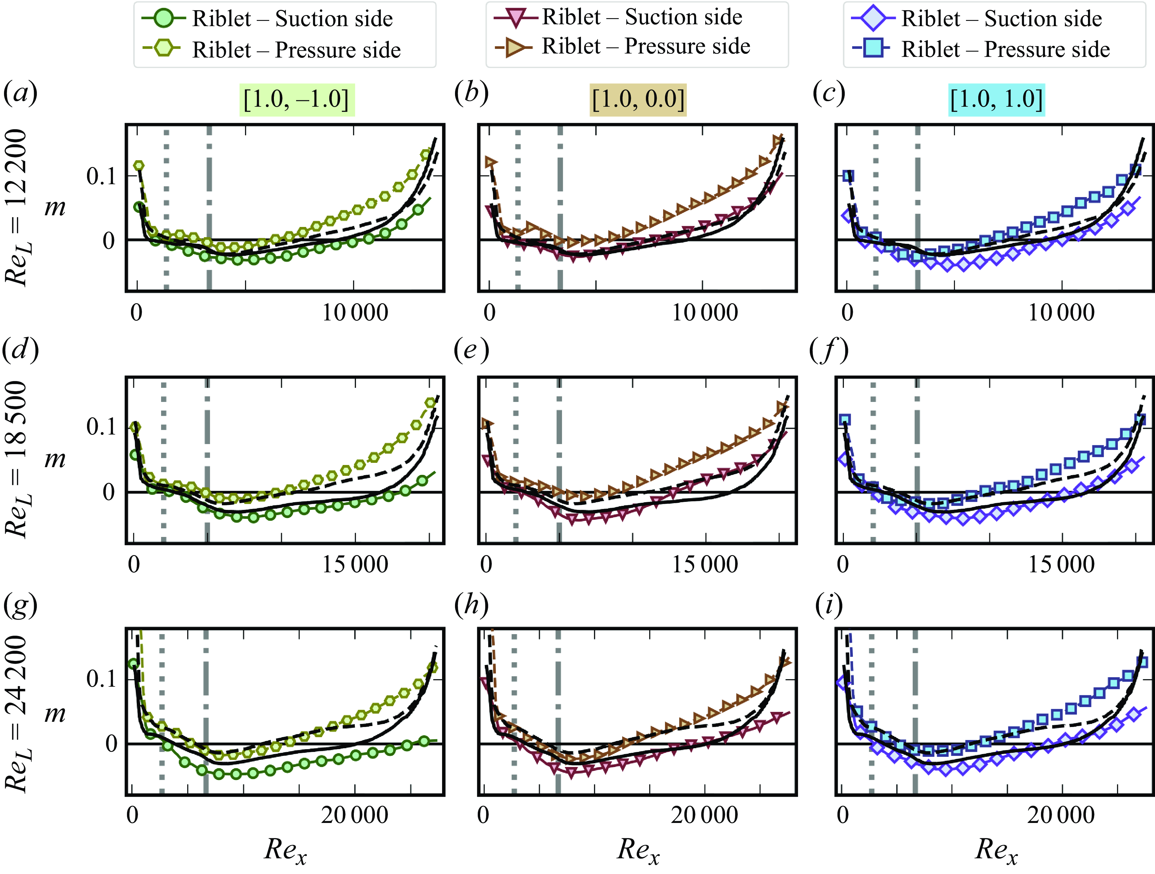
Figure 9. Distribution of $m$
for all the riblet samples of
$m$
for all the riblet samples of ${\mathcal {R}} = 1.0$
and the reference smooth samples on the suction and pressure side for all tested Reynolds numbers. The
${\mathcal {R}} = 1.0$
and the reference smooth samples on the suction and pressure side for all tested Reynolds numbers. The $m$
of the reference smooth sample on the suction and pressure side are shown with solid and dashed black lines, respectively. Locations of
$m$
of the reference smooth sample on the suction and pressure side are shown with solid and dashed black lines, respectively. Locations of $x_{{ LET}}$
and
$x_{{ LET}}$
and $x_{{ Flat}}$
are marked by grey dotted and dash-dotted vertical lines.
$x_{{ Flat}}$
are marked by grey dotted and dash-dotted vertical lines.
3.4.1. Fitting parameter
$m$

The fitting parameter $m$
(presented in figures 9 and SI.5 for all cases) plays a significant role in capturing the local effect of multiple physical phenomena in the flow field; (i) the pressure gradient, (ii) the effect of both the limited (i.e. short) length of the plate and the presence of the riblets on the viscous diffusion, as well as (iii) the effect of the spanwise-averaging operation on the nonlinear advection terms. For all the cases, including the smooth samples, and on both sides, the distribution of
$m$
(presented in figures 9 and SI.5 for all cases) plays a significant role in capturing the local effect of multiple physical phenomena in the flow field; (i) the pressure gradient, (ii) the effect of both the limited (i.e. short) length of the plate and the presence of the riblets on the viscous diffusion, as well as (iii) the effect of the spanwise-averaging operation on the nonlinear advection terms. For all the cases, including the smooth samples, and on both sides, the distribution of $m$
is comprised of three distinct regions: first, a
$m$
is comprised of three distinct regions: first, a $m\gt 0$
region in the leading edge area, then the
$m\gt 0$
region in the leading edge area, then the $m\lt 0$
area in the middle including the location where
$m\lt 0$
area in the middle including the location where $m$
reaches a global minimum and, lastly, the
$m$
reaches a global minimum and, lastly, the $m\gt 0$
for the rest of the length of the plate toward the trailing edge. As is seen in figures 9 and SI.5,
$m\gt 0$
for the rest of the length of the plate toward the trailing edge. As is seen in figures 9 and SI.5, $m$
is larger on the pressure side than the suction side and, as a result, the extent of the
$m$
is larger on the pressure side than the suction side and, as a result, the extent of the $m\lt 0$
region varies quite a bit between the sides and samples, and can take small or large portions of the length of the plate.
$m\lt 0$
region varies quite a bit between the sides and samples, and can take small or large portions of the length of the plate.
In general, $m$
takes a decreasing trend in the early portion of the plate prior to the global minimum and then an increasing trend in the second half toward the trailing edge. The initial decreasing trend is not strictly monotonic for many of the cases on the pressure side; in the LE/LET regions of those, there is a local increasing--decreasing trend that sets in as the flow sees the riblets for the first time. Examples of this are those of [0.5, 0.0] (figure SI.5(Ab)), [0.5, 0.5] (figure SI.5(Ac)), [1.0, −1.0] (figure 9
a) and [1.5, 0.0] (figure SI.5(Cb)) at
$m$
takes a decreasing trend in the early portion of the plate prior to the global minimum and then an increasing trend in the second half toward the trailing edge. The initial decreasing trend is not strictly monotonic for many of the cases on the pressure side; in the LE/LET regions of those, there is a local increasing--decreasing trend that sets in as the flow sees the riblets for the first time. Examples of this are those of [0.5, 0.0] (figure SI.5(Ab)), [0.5, 0.5] (figure SI.5(Ac)), [1.0, −1.0] (figure 9
a) and [1.5, 0.0] (figure SI.5(Cb)) at ${ Re}_{L} = 12\,200$
, [1.0, 0.0] (figure 9
b,e) and [1.5, 1.5] (figure SI.5(Cc,f)) at
${ Re}_{L} = 12\,200$
, [1.0, 0.0] (figure 9
b,e) and [1.5, 1.5] (figure SI.5(Cc,f)) at ${ Re}_{L} = 12\,200$
and
${ Re}_{L} = 12\,200$
and $18\,500$
, and [1.5, –1.5] (figure SI.5(Ca,d,g)) at all the Reynolds numbers.
$18\,500$
, and [1.5, –1.5] (figure SI.5(Ca,d,g)) at all the Reynolds numbers.
In a FS type of BL equation, at a constant Reynolds number, increasing $m$
monotonically increases the wall shear stress, while at a constant
$m$
monotonically increases the wall shear stress, while at a constant $m$
, increasing the Reynolds number monotonically reduces the wall shear stress. Thus, for all the cases, while prior to the minimum
$m$
, increasing the Reynolds number monotonically reduces the wall shear stress. Thus, for all the cases, while prior to the minimum $m$
, the increase in the
$m$
, the increase in the ${ Re}_x$
and decrease in
${ Re}_x$
and decrease in $m$
work together in reducing the
$m$
work together in reducing the $\langle C_f \rangle (x)$
along the length, the evolution of the
$\langle C_f \rangle (x)$
along the length, the evolution of the $m$
past the minimum is the determining factor for the type of shear stress distribution each sample takes. After the minimum
$m$
past the minimum is the determining factor for the type of shear stress distribution each sample takes. After the minimum $m$
, along the length of the sample, the increase in the local Reynolds number results in the wall shear stress decreasing. However, the increase in the
$m$
, along the length of the sample, the increase in the local Reynolds number results in the wall shear stress decreasing. However, the increase in the $m$
disrupts this trend and, depending on the rate of increase of
$m$
disrupts this trend and, depending on the rate of increase of $m$
, the trend in the
$m$
, the trend in the $\langle C_f \rangle (x)$
is set.
$\langle C_f \rangle (x)$
is set.
In the type I distribution, the effect of the rate of increase in $m$
on the
$m$
on the $\langle C_f \rangle (x)$
is not able to overcome the effect of the
$\langle C_f \rangle (x)$
is not able to overcome the effect of the ${ Re}_x$
in decreasing the
${ Re}_x$
in decreasing the $\langle C_f \rangle (x)$
along the length. Thus, overall we see a decreasing trend in the
$\langle C_f \rangle (x)$
along the length. Thus, overall we see a decreasing trend in the $\langle C_f \rangle (x)$
along the length prior to the vicinity of the trailing edge albeit at a lower rate than the region prior to the minimum
$\langle C_f \rangle (x)$
along the length prior to the vicinity of the trailing edge albeit at a lower rate than the region prior to the minimum $m$
and lower than the
$m$
and lower than the ${ Re}_x^{-1/2}$
of the BL theory. However, as seen in figure SI.5(Aa-g) (suction sides) for the
${ Re}_x^{-1/2}$
of the BL theory. However, as seen in figure SI.5(Aa-g) (suction sides) for the ${\mathcal {R}} = 0.5$
family, figure 9(a,b,d,g) (suction sides) for the
${\mathcal {R}} = 0.5$
family, figure 9(a,b,d,g) (suction sides) for the ${\mathcal {R}} = 1.0$
family, and figure SI.5(Cb,e,h) (pressure sides) for the
${\mathcal {R}} = 1.0$
family, and figure SI.5(Cb,e,h) (pressure sides) for the ${\mathcal {R}} = 1.5$
family, the rate of increase in
${\mathcal {R}} = 1.5$
family, the rate of increase in $m$
is faster for the riblets than the smooth reference. This reduces the rate of decrease of
$m$
is faster for the riblets than the smooth reference. This reduces the rate of decrease of $\langle C_f \rangle (x)$
along the length. After the minimum
$\langle C_f \rangle (x)$
along the length. After the minimum $m$
, the
$m$
, the $\unicode{x1D6E5} \langle \tau _{n=0} \rangle /\tau _0$
takes an increasing trend until the vicinity of the trailing edge, at around
$\unicode{x1D6E5} \langle \tau _{n=0} \rangle /\tau _0$
takes an increasing trend until the vicinity of the trailing edge, at around $x/L \approx 0.8$
, where the rate of increase in
$x/L \approx 0.8$
, where the rate of increase in $m$
increases more, leading to
$m$
increases more, leading to $\langle C_f \rangle (x)$
of both the riblet and smooth samples increasing (discussed earlier).
$\langle C_f \rangle (x)$
of both the riblet and smooth samples increasing (discussed earlier).
In the type II distribution, the increase in $m$
nearly balances that of the increase in the
$m$
nearly balances that of the increase in the ${ Re}_x$
, resulting in almost constant
${ Re}_x$
, resulting in almost constant $\langle C_f \rangle (x)$
prior to the trailing edge effect, as seen in the pressure sides of most of the
$\langle C_f \rangle (x)$
prior to the trailing edge effect, as seen in the pressure sides of most of the ${\mathcal {R}} = 0.5$
family (figure SI.5(Aa-h)) and a few cases of the
${\mathcal {R}} = 0.5$
family (figure SI.5(Aa-h)) and a few cases of the ${\mathcal {R}} = 1.0$
family (figure 9
b,c,f,i) and [1.5, 1.5] (figure SI.5(Cc)). The difference between the rate of increase of
${\mathcal {R}} = 1.0$
family (figure 9
b,c,f,i) and [1.5, 1.5] (figure SI.5(Cc)). The difference between the rate of increase of $m$
in type I and II distributions is clearly visible for the suction and pressure sides of the
$m$
in type I and II distributions is clearly visible for the suction and pressure sides of the ${\mathcal {R}} = 0.5$
family at
${\mathcal {R}} = 0.5$
family at ${ Re}_{L} = 12, 200$
and
${ Re}_{L} = 12, 200$
and $18\,500$
(figure SI.5(Aa-f)).
$18\,500$
(figure SI.5(Aa-f)).
In type III and IV distributions, the effect of the increase in $m$
fully overcomes and surpasses that of the local Reynolds number. This results in an increasing (and/or near constant) trend in the
$m$
fully overcomes and surpasses that of the local Reynolds number. This results in an increasing (and/or near constant) trend in the $\langle C_f \rangle (x)$
along the length. Among these two types, the location of the minimum
$\langle C_f \rangle (x)$
along the length. Among these two types, the location of the minimum $m$
is very close to the location of the minimum
$m$
is very close to the location of the minimum $\langle C_{f} \rangle (x)$
. Specifically, for those samples that experience type III or IV on the suction sides, the initial decreasing trend in
$\langle C_{f} \rangle (x)$
. Specifically, for those samples that experience type III or IV on the suction sides, the initial decreasing trend in $m$
along the length of the sample has a faster rate than that of the smooth sample. This results in a larger separation between the minimum
$m$
along the length of the sample has a faster rate than that of the smooth sample. This results in a larger separation between the minimum $m$
of the riblet samples and the smooth reference (for example, see the suction sides of the members of the
$m$
of the riblet samples and the smooth reference (for example, see the suction sides of the members of the ${\mathcal {R}} = 1.5$
family in figure SI.5(Ca-i)). Thus, we see large levels of shear reduction prior to the minimum
${\mathcal {R}} = 1.5$
family in figure SI.5(Ca-i)). Thus, we see large levels of shear reduction prior to the minimum $\langle C_f \rangle (x)$
. Even with the counteracting effect of the increase in
$\langle C_f \rangle (x)$
. Even with the counteracting effect of the increase in ${ Re}_x$
and
${ Re}_x$
and $m$
, after the minimum
$m$
, after the minimum $m$
, these samples can maintain a
$m$
, these samples can maintain a $D_{f}$
-reducing trend on the suction sides. Only on the suction side of the [1.0, 0.0] sample is the rate of increase of
$D_{f}$
-reducing trend on the suction sides. Only on the suction side of the [1.0, 0.0] sample is the rate of increase of $m$
substantially high enough to result in a
$m$
substantially high enough to result in a $D_{f}$
-increasing behaviour.
$D_{f}$
-increasing behaviour.
Overall, the pressure sides of the samples capture larger values of $m$
than the suction sides. With the nonlinear impact of the rate of change of
$m$
than the suction sides. With the nonlinear impact of the rate of change of $m$
on the rate of change in the
$m$
on the rate of change in the $C_f$
(keeping all other parameters constant), we see that while the rate of change of
$C_f$
(keeping all other parameters constant), we see that while the rate of change of $m$
along the length is quite similar between the suction and pressure sides, depending on the sign and magnitude of the
$m$
along the length is quite similar between the suction and pressure sides, depending on the sign and magnitude of the $m$
, this translates into different rates of change in
$m$
, this translates into different rates of change in $\langle C_f \rangle (x)$
between the two sides of the same sample. Mathematically, one can see that as
$\langle C_f \rangle (x)$
between the two sides of the same sample. Mathematically, one can see that as $m$
is increased the variations in the
$m$
is increased the variations in the $C_f$
slowly decreases; for example, increasing
$C_f$
slowly decreases; for example, increasing $m$
from
$m$
from $-0.02$
to
$-0.02$
to $-0.01$
results in a
$-0.01$
results in a $\Delta C_f/ C_f(m=0) = 0.066$
(normalised by the
$\Delta C_f/ C_f(m=0) = 0.066$
(normalised by the $C_f$
of
$C_f$
of $m=0$
FS solution), while increasing
$m=0$
FS solution), while increasing $m$
from 0.01to 0.02 results in
$m$
from 0.01to 0.02 results in $\Delta C_f/ C_f(m=0) = 0.056$
. Thus, comparing the two sides of the samples, with
$\Delta C_f/ C_f(m=0) = 0.056$
. Thus, comparing the two sides of the samples, with $m_{{ pressure}} \geqslant m_{{ suction}}$
, on the pressure sides, the rate of increase in
$m_{{ pressure}} \geqslant m_{{ suction}}$
, on the pressure sides, the rate of increase in $\langle C_f \rangle (x)$
due to the increase in
$\langle C_f \rangle (x)$
due to the increase in $m$
is weaker than on the suction side and, therefore, with the increase in the
$m$
is weaker than on the suction side and, therefore, with the increase in the ${ Re}_x$
, the changes in
${ Re}_x$
, the changes in $\langle C_f \rangle (x)$
on the suction side (as well as the
$\langle C_f \rangle (x)$
on the suction side (as well as the $\unicode{x1D6E5} \langle \tau _{n=0} \rangle /\tau _0$
) show larger variations along the length of the sample compared with those on the pressure sides. This leads to seeing more type I/IV distributions on the suction side (24/27 riblet cases) and more type II distributions on the pressure side (13/27) and a few type IV cases with smaller variations compared with those of the suction sides (8/27)(see figure 8).
$\unicode{x1D6E5} \langle \tau _{n=0} \rangle /\tau _0$
) show larger variations along the length of the sample compared with those on the pressure sides. This leads to seeing more type I/IV distributions on the suction side (24/27 riblet cases) and more type II distributions on the pressure side (13/27) and a few type IV cases with smaller variations compared with those of the suction sides (8/27)(see figure 8).
To explore the effect of $m$
further, we perform the spanwise-averaging operation on the Navier--Stokes equation in the
$m$
further, we perform the spanwise-averaging operation on the Navier--Stokes equation in the $x$
direction for flow past a generic riblet surface and organise and write it in a form resembling that of the BL equation (derivation in § SI.5 of the supplementary material for the Flat region and § SI.6 for the curved LE and LET regions), i.e.
$x$
direction for flow past a generic riblet surface and organise and write it in a form resembling that of the BL equation (derivation in § SI.5 of the supplementary material for the Flat region and § SI.6 for the curved LE and LET regions), i.e.
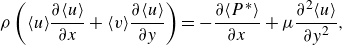 \begin{align} \rho \left ( \langle u \rangle \dfrac {\partial \langle u \rangle }{\partial x} + \langle v \rangle \dfrac {\partial \langle u \rangle }{\partial y} \right ) = - \dfrac {\partial \langle P^{*} \rangle }{\partial x} + \mu \dfrac {\partial ^{2} \langle u \rangle }{\partial y^{2}}, \end{align}
where in the Flat region ( $x\gt x_{{ Flat}}$
)
$x\gt x_{{ Flat}}$
)
 \begin{align} -\dfrac {\partial \langle P^{*} \rangle }{\partial x} = - \underbrace {\dfrac {\partial \langle p \rangle }{\partial x}}_{\unicode {x2460}} + \underbrace {\mu \dfrac {\partial ^{2} \langle u \rangle }{\partial x^{2} } + {\mathcal{Z}}}_{\unicode {x2461}} + \underbrace {\rho \left ( \langle u\rangle \dfrac {\partial \langle u \rangle }{\partial x} + \langle v \rangle \dfrac {\partial \langle u \rangle }{\partial y} - \dfrac {\partial \langle u u \rangle }{\partial x} - \dfrac {\partial \langle u v \rangle }{\partial y} \right )} _{\unicode {x2462}}, \end{align}
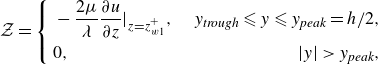 \begin{align} {\mathcal{Z}} = \left \{ \begin{alignedat}{3} & - \dfrac {2\mu }{\lambda } \dfrac {\partial u}{\partial z} \Big \vert _{z=z_{{ w1}}^{+}}, \ \ \ \ \ & y_{\textit{trough}} \leqslant y \leqslant y_{\textit{peak}} = h/2, \\ &0,\ \ \ \ \ &\vert y \vert \gt y_{\textit{peak}}, \end{alignedat} \right . \end{align}
and in the riblet-covered leading edge, LET, ( $x_{{ LET}} \lt x \leqslant x_{{ Flat}}$
)
$x_{{ LET}} \lt x \leqslant x_{{ Flat}}$
)
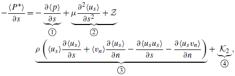 \begin{eqnarray} - \dfrac {\langle P^{*} \rangle }{\partial s} &= & - \underbrace {\dfrac {\partial \langle p \rangle }{\partial s}}_{\unicode {x2460}} + \underbrace {\mu \dfrac {\partial ^{2} \langle u_{s} \rangle }{\partial s^{2}} + {\mathcal{Z}} }_{\unicode {x2461}} \nonumber\\ && \underbrace {\rho \left ( \langle u_{s} \rangle \dfrac {\partial \langle u_{s} \rangle }{\partial s} + \langle v_{n} \rangle \dfrac {\partial \langle u_{s} \rangle }{\partial n} - \dfrac {\partial \langle u_{s} u_{s} \rangle }{\partial s} - \dfrac {\partial \langle u_{s} v_{n} \rangle }{\partial n} \right )}_{\unicode {x2462}} + \underbrace {{\mathcal{K}_2}}_{\unicode {x2463}} , \end{eqnarray}
replacing $y$
with
$y$
with $n$
and
$n$
and $u$
with
$u$
with $u_{s}$
in the definition of the
$u_{s}$
in the definition of the $\mathcal{Z}$
in (3.5), where
$\mathcal{Z}$
in (3.5), where $u_{s}$
and
$u_{s}$
and $v_{n}$
are the tangential and normal velocities along the
$v_{n}$
are the tangential and normal velocities along the $s$
and
$s$
and $n$
directions with respect to the wall of the curved leading edge (see figure 1), and
$n$
directions with respect to the wall of the curved leading edge (see figure 1), and $\mathcal{K}_2$
is the contribution from the curvature of the leading edge as shown in § SI.6 of the supplementary material. In this format, all the excess terms compared with the BL equation are captured via an equivalent pressure gradient term, defined as
$\mathcal{K}_2$
is the contribution from the curvature of the leading edge as shown in § SI.6 of the supplementary material. In this format, all the excess terms compared with the BL equation are captured via an equivalent pressure gradient term, defined as $\partial \langle P^{*} \rangle / \partial x$
(or
$\partial \langle P^{*} \rangle / \partial x$
(or $\partial \langle P^{*} \rangle / \partial s$
), so that (3.3) matches the form of the FS family of BL equations.
$\partial \langle P^{*} \rangle / \partial s$
), so that (3.3) matches the form of the FS family of BL equations.
Here, locally, by fitting the collected data to the FS equations, we capture the $\partial \langle P^{*} \rangle /\partial x$
term via the
$\partial \langle P^{*} \rangle /\partial x$
term via the $m$
parameter that is then written in the form of
$m$
parameter that is then written in the form of $-{\partial \langle P^{*} \rangle }/{\partial x} = \rho U(x)^{2} {m}/{x}$
, where the distribution of this term follows the same trend as the
$-{\partial \langle P^{*} \rangle }/{\partial x} = \rho U(x)^{2} {m}/{x}$
, where the distribution of this term follows the same trend as the $m$
and the
$m$
and the $1/x$
acts as a scaling factor that decreases along the length. Note that, as mentioned in § 2.4.2, for simplicity, in the LE and LET, we perform the fitting with
$1/x$
acts as a scaling factor that decreases along the length. Note that, as mentioned in § 2.4.2, for simplicity, in the LE and LET, we perform the fitting with $x$
instead of
$x$
instead of $s$
and let
$s$
and let $m$
also capture the effect of this difference and, thus, use
$m$
also capture the effect of this difference and, thus, use $-{\partial \langle P^{*} \rangle }/{\partial s} = \rho U(x)^{2} {m}/{x}$
in the curved leading edge area. Thus, the
$-{\partial \langle P^{*} \rangle }/{\partial s} = \rho U(x)^{2} {m}/{x}$
in the curved leading edge area. Thus, the $m$
parameterrepresents the cumulative effect of
$m$
parameterrepresents the cumulative effect of $\unicode {x2460}$
the pressure gradient,
$\unicode {x2460}$
the pressure gradient, $\unicode {x2461}$
the non-negligible viscous diffusion term in the
$\unicode {x2461}$
the non-negligible viscous diffusion term in the $x$
direction and the viscous diffusion term in the
$x$
direction and the viscous diffusion term in the $z$
direction due to the three-dimensional effect inside the grooves, as well as
$z$
direction due to the three-dimensional effect inside the grooves, as well as $\unicode {x2462}$
the residues from the nonlinear terms left from the averaging operation. In the leading edge area,
$\unicode {x2462}$
the residues from the nonlinear terms left from the averaging operation. In the leading edge area, $m$
also captures the effect of the curvature both through the
$m$
also captures the effect of the curvature both through the $\mathcal{K}_2$
term (see § SI.6 of the supplementary material) and the use of
$\mathcal{K}_2$
term (see § SI.6 of the supplementary material) and the use of $x$
in the fitting process. In the LEarea, (3.3) turns back into (see § SI.6)
$x$
in the fitting process. In the LEarea, (3.3) turns back into (see § SI.6)
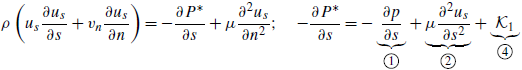 \begin{align} \rho \left ( u_{s} \dfrac {\partial u_{s} }{\partial s} + v_{n} \dfrac {\partial u_{s} }{\partial n} \right ) = - \dfrac {\partial P^{*} }{\partial s} + \mu \dfrac {\partial ^{2} u_{s} }{\partial n^{2}}; \quad -\dfrac {\partial P^{*} }{\partial s} = - \underbrace {\dfrac { \partial p }{\partial s}}_{\unicode {x2460}} + \underbrace {\mu \dfrac {\partial ^{2} u_{s} }{\partial s^{2} }}_{\unicode {x2461}} + \underbrace { {{\mathcal{K}}_1} }_{\unicode {x2463}} \end{align}
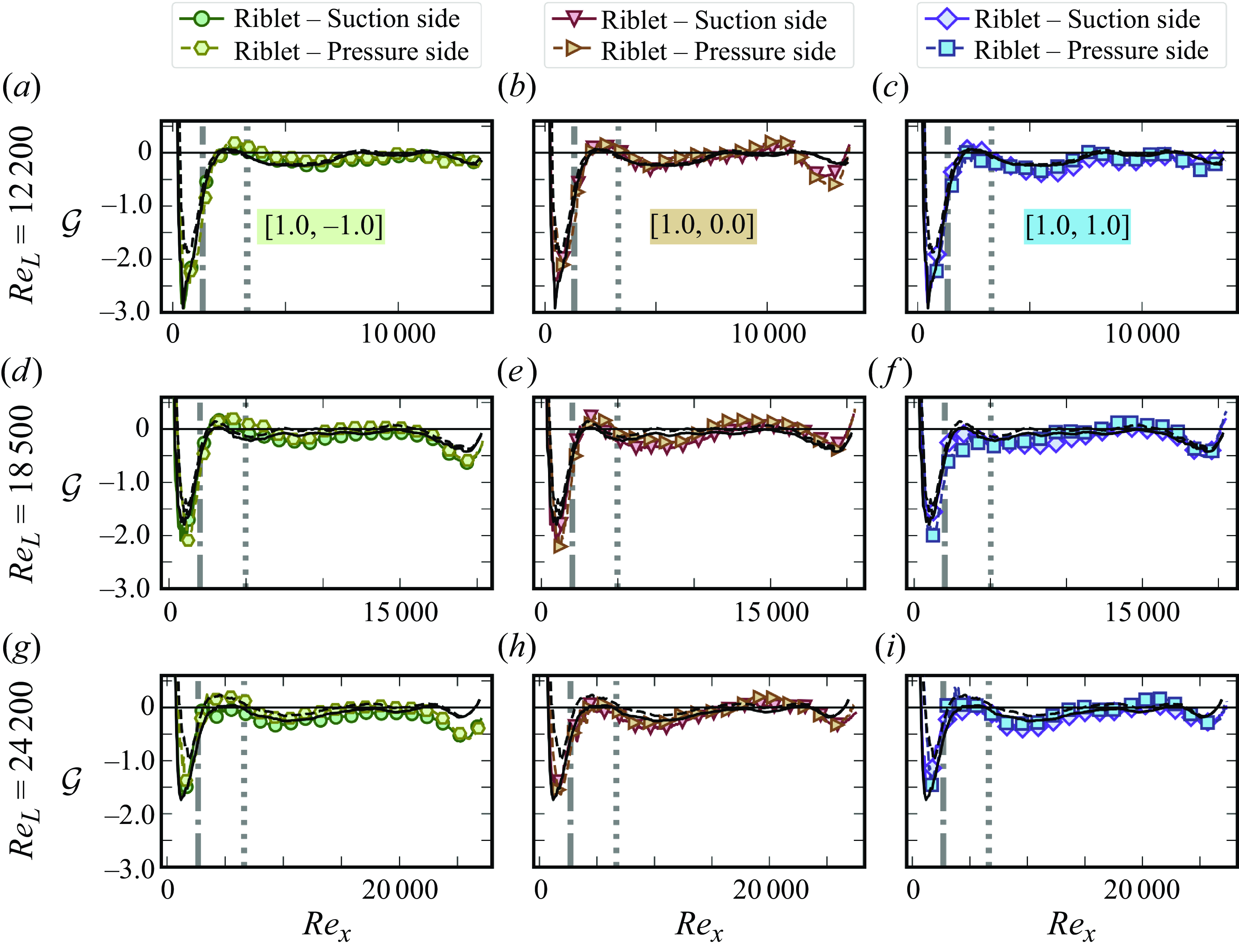
Figure 10. Distribution of ${\mathcal {G}}$
or difference between the
${\mathcal {G}}$
or difference between the $\partial \langle P^{*} \rangle /\partial x$
and
$\partial \langle P^{*} \rangle /\partial x$
and $\partial \langle p \rangle /\partial x$
terms in dimensionless form for all the riblet samples of
$\partial \langle p \rangle /\partial x$
terms in dimensionless form for all the riblet samples of ${\mathcal {R}} = 1.0$
on the suction and pressure side of the riblet samples. The results for the smooth reference for all the tested Reynolds numbers are shown with solid and dashed black lines for the suction and pressure sides, respectively. Locations of
${\mathcal {R}} = 1.0$
on the suction and pressure side of the riblet samples. The results for the smooth reference for all the tested Reynolds numbers are shown with solid and dashed black lines for the suction and pressure sides, respectively. Locations of $x_{{ LET}}$
and
$x_{{ LET}}$
and $x_{{ Flat}}$
are marked by grey dotted and dash-dotted vertical lines.
$x_{{ Flat}}$
are marked by grey dotted and dash-dotted vertical lines.
as expected, missing the $\unicode {x2462}$
term compared with the riblet regions with
$\unicode {x2462}$
term compared with the riblet regions with $-{\partial P^{*}}/{\partial s} = \rho U(x)^{2} ({m}/{x})$
. Separate from the curve fitting operation, we use the PIV data and find the pressure gradient following § 2.4.3 and find the dimensionless pressure gradient terms in the form of
$-{\partial P^{*}}/{\partial s} = \rho U(x)^{2} ({m}/{x})$
. Separate from the curve fitting operation, we use the PIV data and find the pressure gradient following § 2.4.3 and find the dimensionless pressure gradient terms in the form of
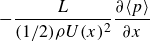 \begin{align} -\dfrac {L}{({1}/{2}) \rho U(x)^{2}} \dfrac {\partial \langle p \rangle }{\partial x} \end{align}
on a horizontal line parallel to the Flat portion of the samples at a height of $y = \pm 0.6 h$
, which is at a distance of
$y = \pm 0.6 h$
, which is at a distance of $0.1 h$
or
$0.1 h$
or $\lambda /2$
from the Flat part of the surface on either side, where the three-dimensional effects of the riblets have mostly faded away and it is safe to assume that
$\lambda /2$
from the Flat part of the surface on either side, where the three-dimensional effects of the riblets have mostly faded away and it is safe to assume that $\mathbf{u}(x,y,z) = \langle \mathbf{u} \rangle (x,y)$
and
$\mathbf{u}(x,y,z) = \langle \mathbf{u} \rangle (x,y)$
and $p(x,y,z) = \langle p \rangle (x,y)$
. Therefore, we can find the difference between the
$p(x,y,z) = \langle p \rangle (x,y)$
. Therefore, we can find the difference between the $\partial \langle p \rangle /\partial x$
and
$\partial \langle p \rangle /\partial x$
and $\partial \langle P^{*} \rangle /\partial x$
, corresponding to terms
$\partial \langle P^{*} \rangle /\partial x$
, corresponding to terms $\unicode {x2461}$
and
$\unicode {x2461}$
and $\unicode {x2462}$
(as well as
$\unicode {x2462}$
(as well as $\unicode {x2463}$
in the LE and LET regions), found via the two separate methods, in a dimensionless form as
$\unicode {x2463}$
in the LE and LET regions), found via the two separate methods, in a dimensionless form as
 \begin{align} {\mathcal {G}} = \dfrac {-L}{(1/2) \rho U(x)^{2}} \left ( \dfrac {\partial \langle P^*\rangle }{\partial x} - \dfrac {\partial \langle p \rangle }{\partial x} \right ) = \dfrac {2mL}{x} + \dfrac {L}{({1}/{2}) \rho U(x)^{2}} \dfrac {\partial \langle p \rangle }{\partial x} \end{align}
and present it for all the riblet samples in figures 10 and SI.7, with the results for the smooth sample shown as reference. (In the LE and LET regions the $\partial /\partial s$
has been transformed to
$\partial /\partial s$
has been transformed to $\partial /\partial x$
using the chain rule
$\partial /\partial x$
using the chain rule $\partial /\partial x = \partial s/\partial x \ \partial /\partial s$
.) As seen in this figure, the non-zero difference between the two terms confirms that the
$\partial /\partial x = \partial s/\partial x \ \partial /\partial s$
.) As seen in this figure, the non-zero difference between the two terms confirms that the $\unicode {x2461}$
,
$\unicode {x2461}$
, $\unicode {x2462}$
and
$\unicode {x2462}$
and $\unicode {x2463}$
have limited non-negligible effects for a finite length sample. Firstly, in the absence of the riblets for the smooth reference, in the LE and LET regions, (3.7) holds while in the Flat region, (3.3) and (3.4) are simplified to
$\unicode {x2463}$
have limited non-negligible effects for a finite length sample. Firstly, in the absence of the riblets for the smooth reference, in the LE and LET regions, (3.7) holds while in the Flat region, (3.3) and (3.4) are simplified to
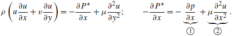 \begin{align} \rho \left ( u \dfrac {\partial u }{\partial x} + v \dfrac {\partial u }{\partial y} \right ) = - \dfrac {\partial P^{*} }{\partial x} + \mu \dfrac {\partial ^{2} u }{\partial y^{2}} ; \qquad -\dfrac {\partial P^{*} }{\partial x} = - \underbrace {\dfrac { \partial p }{\partial x}}_{\unicode {x2460}} + \underbrace {\mu \dfrac {\partial ^{2} u }{\partial x^{2} }}_{\unicode {x2461}}. \\[-18pt] \nonumber \end{align}
The viscous term in the streamwise direction, $\unicode {x2461}$
, as seen in figures 10 and SI.7is mostly zero or negative along both sides of the plate in the Flat region. In the leading edge area, the effect of both
$\unicode {x2461}$
, as seen in figures 10 and SI.7is mostly zero or negative along both sides of the plate in the Flat region. In the leading edge area, the effect of both $\unicode {x2461}$
and
$\unicode {x2461}$
and $\unicode {x2463}$
are present and, hence,
$\unicode {x2463}$
are present and, hence, ${\mathcal {G}}$
captures its largest deviation from zero and stays mostly negative. Since the smooth surface (of the configuration used here) does not experience any form of flow reversal, we do not expect
${\mathcal {G}}$
captures its largest deviation from zero and stays mostly negative. Since the smooth surface (of the configuration used here) does not experience any form of flow reversal, we do not expect $\unicode {x2461}$
to become positive for this sample and, thus, the small regions of
$\unicode {x2461}$
to become positive for this sample and, thus, the small regions of ${\mathcal {G}}\gt 0$
in the LE and LET are most likely due to the contributions from the curvature terms
${\mathcal {G}}\gt 0$
in the LE and LET are most likely due to the contributions from the curvature terms $\unicode {x2463}$
.
$\unicode {x2463}$
.
Moving to the riblet-covered samples, the distribution of ${\mathcal {G}}$
follows a very similar trend to that of the smooth surface, and especially for the shallowest riblets of the
${\mathcal {G}}$
follows a very similar trend to that of the smooth surface, and especially for the shallowest riblets of the ${\mathcal {R}} = 0.5$
family (figure SI.7(A)), the distributions are nearly the same with slight differences recorded for the
${\mathcal {R}} = 0.5$
family (figure SI.7(A)), the distributions are nearly the same with slight differences recorded for the ${ Re}_{L} = 18\,500$
cases in the early portions of the Flat region. Similarly, for all the cases, in the LE region,
${ Re}_{L} = 18\,500$
cases in the early portions of the Flat region. Similarly, for all the cases, in the LE region, ${\mathcal {G}}$
is nearly the same as that of the smooth reference and in the LET region slight differences can be seen for members ofthe
${\mathcal {G}}$
is nearly the same as that of the smooth reference and in the LET region slight differences can be seen for members ofthe ${\mathcal {R}} = 1.0$
and
${\mathcal {R}} = 1.0$
and $1.5$
families (figures 10 and SI.7(C)), which could be due to any of the
$1.5$
families (figures 10 and SI.7(C)), which could be due to any of the $\unicode {x2461}$
,
$\unicode {x2461}$
, $\unicode {x2462}$
or
$\unicode {x2462}$
or $\unicode {x2463}$
terms.
$\unicode {x2463}$
terms.
The main differences between the ${\mathcal {G}}$
of the smooth and riblet surfaces in the Flat region is seen among the
${\mathcal {G}}$
of the smooth and riblet surfaces in the Flat region is seen among the ${\mathcal {R}} = 1.0$
and
${\mathcal {R}} = 1.0$
and $1.5$
families. For example, in the early portion of the Flat region of [1.5, 1.5] at all Reynolds numbers (figure SI.7(Cc,f,i)) and [1.5, 0.0], [1.5, -1.5], [1.0, 1.0] and [1.0, 0.0] at Reynolds numbers of
$1.5$
families. For example, in the early portion of the Flat region of [1.5, 1.5] at all Reynolds numbers (figure SI.7(Cc,f,i)) and [1.5, 0.0], [1.5, -1.5], [1.0, 1.0] and [1.0, 0.0] at Reynolds numbers of $18\,500$
and
$18\,500$
and $24\,200$
(figures SI.7(Cd,e,g,h) and 10(e,f,h,i),
$24\,200$
(figures SI.7(Cd,e,g,h) and 10(e,f,h,i), ${\mathcal {G}}$
is lower than that of the smooth one. This is due to the effect of both
${\mathcal {G}}$
is lower than that of the smooth one. This is due to the effect of both $\unicode {x2462}$
and contributions from the
$\unicode {x2462}$
and contributions from the $\mathcal{Z}$
terms. In the latter portion of the Flat region, especially for samples [1.0, 0.0], [1.0, 1.0], [1.5, -1.5] and [1.5, 1.5], unlike the smooth reference,
$\mathcal{Z}$
terms. In the latter portion of the Flat region, especially for samples [1.0, 0.0], [1.0, 1.0], [1.5, -1.5] and [1.5, 1.5], unlike the smooth reference, ${\mathcal {G}}$
turns positive for some extent of the plate length. In this region, as the flow inside the grooves has had sufficient distance to develop, it is more likely for the slow down inside the riblets to lead to near stagnant flow inside the grooves with potential for small recirculation regions (Raayai-Ardakani & McKinley Reference Raayai-Ardakani and McKinley2017) turning the viscous terms
${\mathcal {G}}$
turns positive for some extent of the plate length. In this region, as the flow inside the grooves has had sufficient distance to develop, it is more likely for the slow down inside the riblets to lead to near stagnant flow inside the grooves with potential for small recirculation regions (Raayai-Ardakani & McKinley Reference Raayai-Ardakani and McKinley2017) turning the viscous terms $\unicode {x2461}$
positive, and giving more weight to the contributions of
$\unicode {x2461}$
positive, and giving more weight to the contributions of $\unicode {x2461}$
than
$\unicode {x2461}$
than $\unicode {x2462}$
here (see more in the upcoming § 3.4.2). The difference tends to become more visible toward the sharpest textures and also toward samples with larger
$\unicode {x2462}$
here (see more in the upcoming § 3.4.2). The difference tends to become more visible toward the sharpest textures and also toward samples with larger $\kappa _2$
where the available cross-sectional area within the riblets allows for
$\kappa _2$
where the available cross-sectional area within the riblets allows for $\unicode {x2461}$
and
$\unicode {x2461}$
and $\unicode {x2462}$
terms to capture larger variations and push
$\unicode {x2462}$
terms to capture larger variations and push ${\mathcal {G}}$
to deviate from that of the smooth reference. These cases experience type II, III (all) and IV shear distributions.
${\mathcal {G}}$
to deviate from that of the smooth reference. These cases experience type II, III (all) and IV shear distributions.
Overall, the similarity of the $\mathcal{G}$
of the riblet and smooth samples and the order of magnitude of the difference observed between the two gives us confidence that the spanwise-averaging operation is able to capture a large part of the flow dynamics and is a credible method for extracting valuable information in studying the effect of riblets and the three-dimensional nature of the flow inside their grooves.
$\mathcal{G}$
of the riblet and smooth samples and the order of magnitude of the difference observed between the two gives us confidence that the spanwise-averaging operation is able to capture a large part of the flow dynamics and is a credible method for extracting valuable information in studying the effect of riblets and the three-dimensional nature of the flow inside their grooves.
3.4.2. The effective origin,
$n_0$

The distribution of the $n_0$
for the suction and pressure sides of all the riblet samples and for all the tested Reynolds numbers are shown in figures 11 and SI.8. In all the plots, the design location of the trough of the riblets and the measured locations are shown for comparison and the
$n_0$
for the suction and pressure sides of all the riblet samples and for all the tested Reynolds numbers are shown in figures 11 and SI.8. In all the plots, the design location of the trough of the riblets and the measured locations are shown for comparison and the $n_0$
values are normalised with
$n_0$
values are normalised with $\lambda /2$
, which is the more consistent dimensions among all the printed samples. For the majority of the cases tested, the distributions of
$\lambda /2$
, which is the more consistent dimensions among all the printed samples. For the majority of the cases tested, the distributions of $n_0$
, on both sides of the samples, follow a non-monotonic behaviour where initially, following the growth of the riblet height in the LETregion, the magnitude of the effective origin increases, reaching a maximum in the early portions of the Flat region, before decreasing to a non-zero minimum. Afterward again increasing in the vicinity of the trailing edge of the samples until the end of the body. In a few of the cases, namely the suction side of [0.5, 0.5] at
$n_0$
, on both sides of the samples, follow a non-monotonic behaviour where initially, following the growth of the riblet height in the LETregion, the magnitude of the effective origin increases, reaching a maximum in the early portions of the Flat region, before decreasing to a non-zero minimum. Afterward again increasing in the vicinity of the trailing edge of the samples until the end of the body. In a few of the cases, namely the suction side of [0.5, 0.5] at ${ Re}_{L} = 12\,200$
(figure SI.8(Ac)), the pressure side of [1.0, -1.0] at
${ Re}_{L} = 12\,200$
(figure SI.8(Ac)), the pressure side of [1.0, -1.0] at ${ Re}_{L} = 12\,200$
(figure 11
a) and the suction side of [1.0, −1.0] at
${ Re}_{L} = 12\,200$
(figure 11
a) and the suction side of [1.0, −1.0] at ${ Re}_{L} = 18\,500$
(figure 11
d), after the initial increase in the magnitude
${ Re}_{L} = 18\,500$
(figure 11
d), after the initial increase in the magnitude $n_0$
, in the Flat region, the effective origin stays nearly constant for a portion of the length of the sample until close to the trailing edge where
$n_0$
, in the Flat region, the effective origin stays nearly constant for a portion of the length of the sample until close to the trailing edge where $n_0$
increases toward the end of the plate. In all the cases, the magnitudes of the
$n_0$
increases toward the end of the plate. In all the cases, the magnitudes of the $n_0$
on the suction sides are larger than or similar to the pressure sides.
$n_0$
on the suction sides are larger than or similar to the pressure sides.
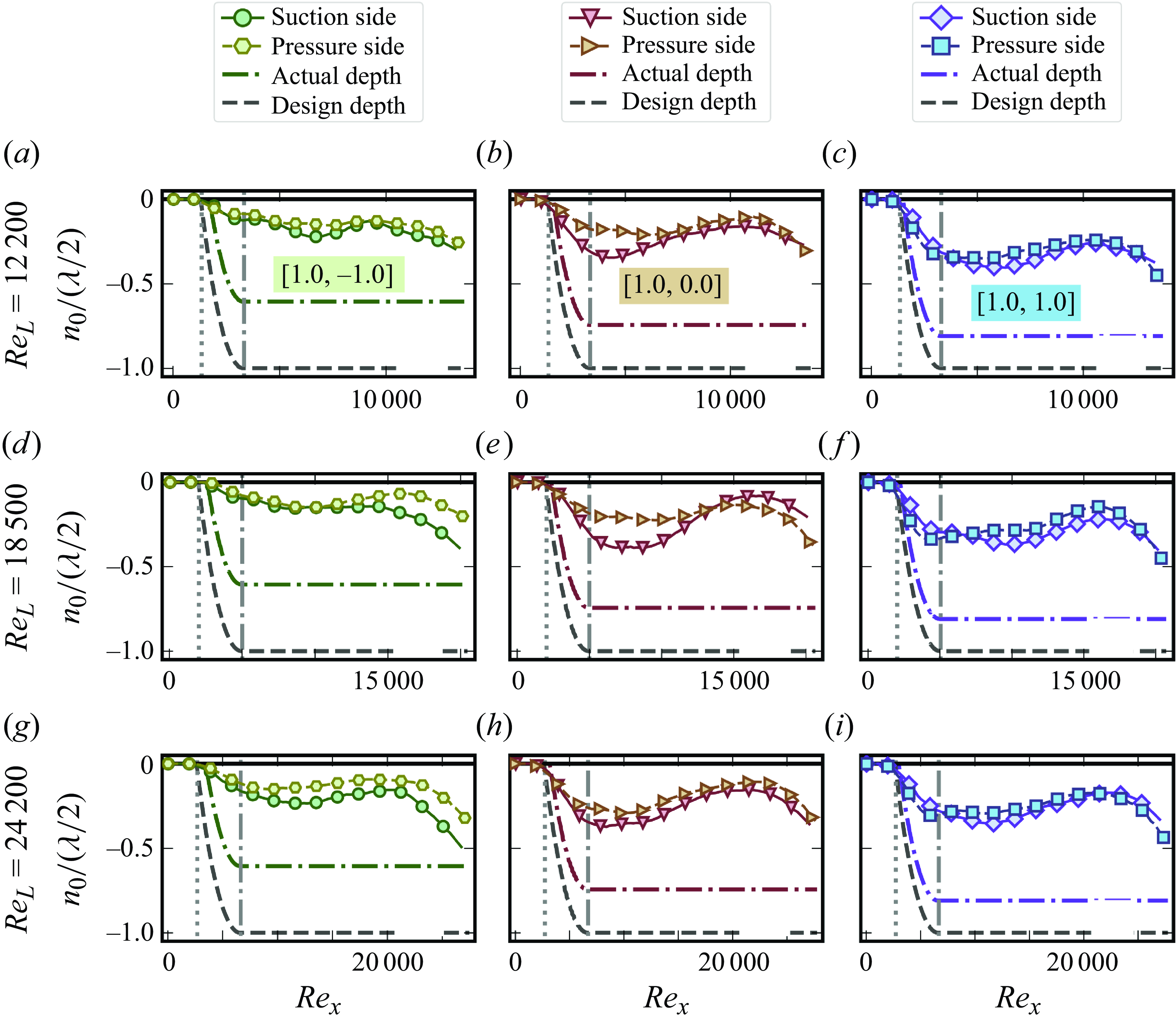
Figure 11. Distribution of the effective origin, $n_0$
, for all the riblet samples of
$n_0$
, for all the riblet samples of ${\mathcal {R}} = 1.0$
on the suction and pressure side for all tested Reynolds numbers. The location of the design and measured troughs are also marked on the figures. Locations of
${\mathcal {R}} = 1.0$
on the suction and pressure side for all tested Reynolds numbers. The location of the design and measured troughs are also marked on the figures. Locations of $x_{{ LET}}$
and
$x_{{ LET}}$
and $x_{{ Flat}}$
are marked by grey dotted and dash-dotted vertical lines.
$x_{{ Flat}}$
are marked by grey dotted and dash-dotted vertical lines.
Generally, within the ${\mathcal {R}} =$
constant families, at a constant Reynolds number, the magnitude of the
${\mathcal {R}} =$
constant families, at a constant Reynolds number, the magnitude of the $n_0$
tends to be larger for
$n_0$
tends to be larger for $\kappa _2={\mathcal {R}}$
(concave) and
$\kappa _2={\mathcal {R}}$
(concave) and $\kappa _2 = 0.0$
(triangular) where there is a larger cross-sectional area available in the riblets for the flow to develop compared with the convex ones. Additionally, as the global Reynolds number is increased, we see the absolute values of
$\kappa _2 = 0.0$
(triangular) where there is a larger cross-sectional area available in the riblets for the flow to develop compared with the convex ones. Additionally, as the global Reynolds number is increased, we see the absolute values of $n_0$
slightly increasing in the early portion of the Flat region. As expected, as
$n_0$
slightly increasing in the early portion of the Flat region. As expected, as ${\mathcal {R}}$
is increased and the available depth of the riblets increases, the effective origin of the velocity profiles is also found to be larger, especially for the concave
${\mathcal {R}}$
is increased and the available depth of the riblets increases, the effective origin of the velocity profiles is also found to be larger, especially for the concave $\kappa _2 = {\mathcal {R}}$
cases. Among the
$\kappa _2 = {\mathcal {R}}$
cases. Among the ${\mathcal {R}} = 0.5$
family, for all Reynolds numbers and on both sides, the
${\mathcal {R}} = 0.5$
family, for all Reynolds numbers and on both sides, the $n_0$
of the [0.5, 0.0] and [0.5, 0.0] samples have similar magnitudes in the LET and early portion of the Flat region and toward the second half, the magnitude of the
$n_0$
of the [0.5, 0.0] and [0.5, 0.0] samples have similar magnitudes in the LET and early portion of the Flat region and toward the second half, the magnitude of the $n_0$
of the [0.5, 0.5] sample becomes larger than the [0.5, 0.0] sample. Owing to the limited resolution of the three-dimensional printer (as listed in table 1), while the height of all the samples are smaller than their design height, the height of the [0.5, 0.5] sample is slightly smaller than the other two samples and, thus, for this sample, the magnitude of
$n_0$
of the [0.5, 0.5] sample becomes larger than the [0.5, 0.0] sample. Owing to the limited resolution of the three-dimensional printer (as listed in table 1), while the height of all the samples are smaller than their design height, the height of the [0.5, 0.5] sample is slightly smaller than the other two samples and, thus, for this sample, the magnitude of $n_0$
can reach to a maximum of between
$n_0$
can reach to a maximum of between $53\,\%\!-\!70\,\%/39\,\%\!-\!60\,\%$
of the measured
$53\,\%\!-\!70\,\%/39\,\%\!-\!60\,\%$
of the measured $A$
in the middle of the suction/pressure side of the riblets. For the [0.5, 0.0] and [0.5, -0.5]samples, the depth of
$A$
in the middle of the suction/pressure side of the riblets. For the [0.5, 0.0] and [0.5, -0.5]samples, the depth of $n_0$
reaches between
$n_0$
reaches between $50\,\%\!-\!64\,\%/38\,\%\!-\!46\,\%$
and
$50\,\%\!-\!64\,\%/38\,\%\!-\!46\,\%$
and $38\,\%\!-\!53\,\%/24\,\%\!-\!41\,\%$
of their respective measured
$38\,\%\!-\!53\,\%/24\,\%\!-\!41\,\%$
of their respective measured $A$
in the middle of the suction/pressure sides. As the depth of the samples (i.e.
$A$
in the middle of the suction/pressure sides. As the depth of the samples (i.e. ${\mathcal {R}}$
) increases, while we see the absolute value of
${\mathcal {R}}$
) increases, while we see the absolute value of $n_0$
slightly increasing, the ratio of
$n_0$
slightly increasing, the ratio of $\vert n_0 \vert /A$
keeps decreasing. For the
$\vert n_0 \vert /A$
keeps decreasing. For the ${\mathcal {R}} = 1.5$
family, on the suction/pressure sides the
${\mathcal {R}} = 1.5$
family, on the suction/pressure sides the $\vert n_0 \vert /A$
can reach as high as
$\vert n_0 \vert /A$
can reach as high as $43\,\%/33\,\%$
as seen for the [1.5, 1.5] sample. Similarly, for the
$43\,\%/33\,\%$
as seen for the [1.5, 1.5] sample. Similarly, for the ${\mathcal {R}} = 1.0$
family, on the suction/pressure sides, the maximum
${\mathcal {R}} = 1.0$
family, on the suction/pressure sides, the maximum $\vert n_0 \vert /A$
in the middle of the plate is found to be around
$\vert n_0 \vert /A$
in the middle of the plate is found to be around $50\,\%/42\,\%$
, respectively. As a result, for sharper riblets, we expect that a larger volume of the fluid inside the grooves to be ina near stagnant condition compared with the shallower grooves where the effective origin can penetrate more than
$50\,\%/42\,\%$
, respectively. As a result, for sharper riblets, we expect that a larger volume of the fluid inside the grooves to be ina near stagnant condition compared with the shallower grooves where the effective origin can penetrate more than $50\,\%$
of the height of the riblet.
$50\,\%$
of the height of the riblet.
The trend in the effective origin, $n_0$
, of the spanwise-averaged velocity profiles in the streamwise direction can be explained further with the idea of flow retardation inside the grooves (key drag reduction mechanism in the laminar regimes) that leads to the creation of a layer of stagnant (or slow-moving) fluid (figure 12), which has been shown in previous numerical simulations (Chu & Karniadakis Reference Chu and Karniadakis1993; Choi et al. Reference Choi, Moin and Kim1993; Raayai-Ardakani & McKinley Reference Raayai-Ardakani and McKinley2017). Here, as the BL develops along the plate and inside the riblets, the magnitude of the effective origin of the
$n_0$
, of the spanwise-averaged velocity profiles in the streamwise direction can be explained further with the idea of flow retardation inside the grooves (key drag reduction mechanism in the laminar regimes) that leads to the creation of a layer of stagnant (or slow-moving) fluid (figure 12), which has been shown in previous numerical simulations (Chu & Karniadakis Reference Chu and Karniadakis1993; Choi et al. Reference Choi, Moin and Kim1993; Raayai-Ardakani & McKinley Reference Raayai-Ardakani and McKinley2017). Here, as the BL develops along the plate and inside the riblets, the magnitude of the effective origin of the $\langle u \rangle$
(or
$\langle u \rangle$
(or $\langle u_{s} \rangle$
) profiles slowly increases until reaching a maximum. From this point, first a layer of slow-moving fluid starts to develop inside the grooves and grows along the length of the plate. This layer due to its near-zero velocity does not communicate with the rest of the flow and acts as a blockage, pushing the moving fluid to the outside, effectively squeezing the flow between the higher
$\langle u_{s} \rangle$
) profiles slowly increases until reaching a maximum. From this point, first a layer of slow-moving fluid starts to develop inside the grooves and grows along the length of the plate. This layer due to its near-zero velocity does not communicate with the rest of the flow and acts as a blockage, pushing the moving fluid to the outside, effectively squeezing the flow between the higher $n_0$
and the inviscid outer flow and at times leading to a faster rate of increase in
$n_0$
and the inviscid outer flow and at times leading to a faster rate of increase in $m$
. This moves the location of
$m$
. This moves the location of $n_0$
outward resulting in a decrease in the magnitude of the
$n_0$
outward resulting in a decrease in the magnitude of the $n_0$
. This continues until close to the vicinity of the trailing edge where the velocity in the
$n_0$
. This continues until close to the vicinity of the trailing edge where the velocity in the $y$
direction,
$y$
direction, $v$
, outside the grooves changes direction toward the sample (instead of away from the sample; see figure 6
f) and effectively pushes the flow inside the grooves and increases the magnitude of
$v$
, outside the grooves changes direction toward the sample (instead of away from the sample; see figure 6
f) and effectively pushes the flow inside the grooves and increases the magnitude of $n_0$
. In this region, the flow is more attached to the surface with larger
$n_0$
. In this region, the flow is more attached to the surface with larger $m$
values (as seen in § 3.4.1), and also larger values of
$m$
values (as seen in § 3.4.1), and also larger values of $\langle C_f \rangle (x)$
than the earlier parts of the Flat region where the magnitude of
$\langle C_f \rangle (x)$
than the earlier parts of the Flat region where the magnitude of $n_0$
reaches a local maximum (as discussed in § 3.3).
$n_0$
reaches a local maximum (as discussed in § 3.3).
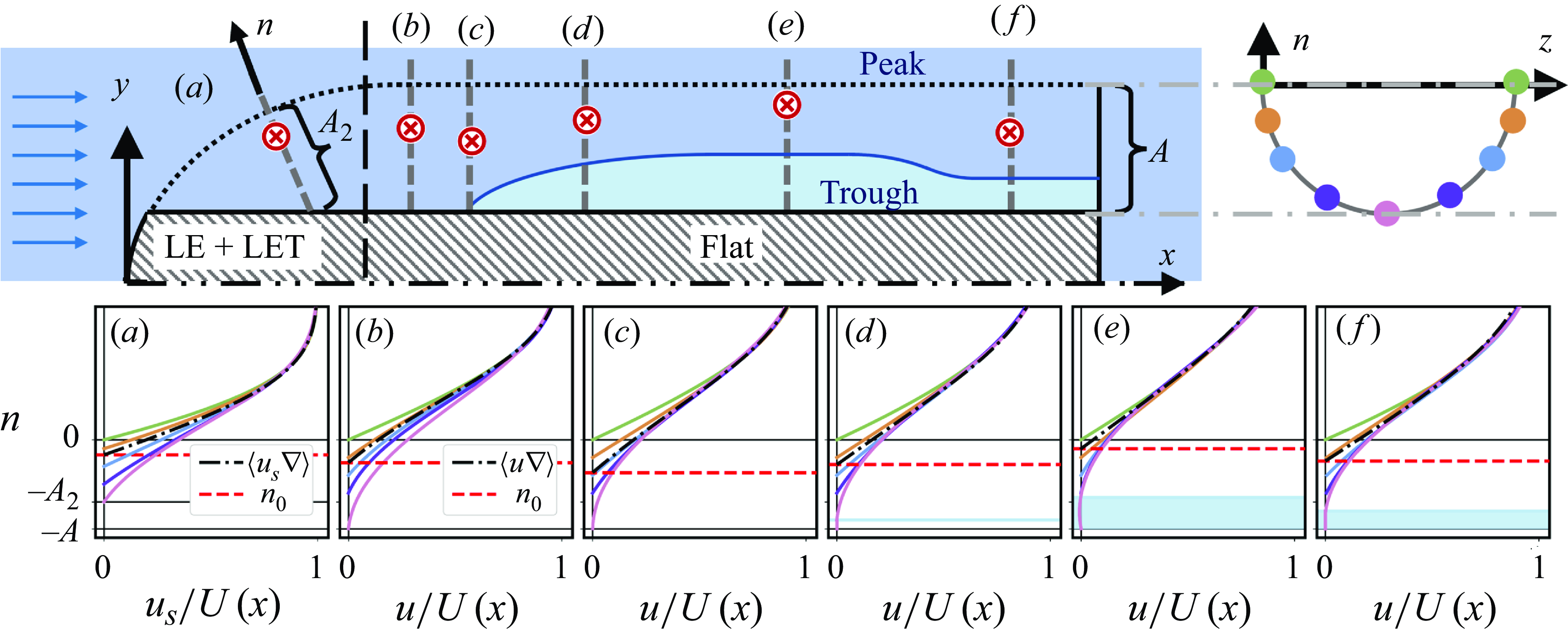
Figure 12. Schematic rendering of the evolution of the effective origin of the velocity profiles (top left) along the grooves of riblet samples for a hypothetical riblet (top right) and the respective local velocity profiles at five points (and their mirror images, as shown on the top-right riblet profile with dots with the same colours) in the spanwise direction of the riblet and their respective $\langle u \rangle$
at streamwise locations (a--f) along the sample.
$\langle u \rangle$
at streamwise locations (a--f) along the sample.
In some cases, the quiescent flow layer can lead to a slight recirculation in the flow (Raayai-Ardakani & McKinley Reference Raayai-Ardakani and McKinley2017), which can result in the viscous diffusion terms in $\unicode {x2461}$
of (3.4) to become positive, leading to
$\unicode {x2461}$
of (3.4) to become positive, leading to ${\mathcal {G}}\gt 0$
in the latter part of the sample as seen in § 3.4.1. Comparing figures 11, SI.8, 10 and SI.7, one can see that, for cases with
${\mathcal {G}}\gt 0$
in the latter part of the sample as seen in § 3.4.1. Comparing figures 11, SI.8, 10 and SI.7, one can see that, for cases with ${\mathcal {G}}\gt 0$
areas in the Flat region, the
${\mathcal {G}}\gt 0$
areas in the Flat region, the ${\mathcal {G}}\gt 0$
region is very close to where the magnitude of the
${\mathcal {G}}\gt 0$
region is very close to where the magnitude of the $n_0$
reaches a local minimum. In this region, with a very slow-moving fluid inside the grooves, the contribution from term
$n_0$
reaches a local minimum. In this region, with a very slow-moving fluid inside the grooves, the contribution from term $\unicode {x2462}$
is likely very small and
$\unicode {x2462}$
is likely very small and ${\mathcal {G}}$
becoming even slightly positive can serve as an indication of the potential for existence of flow reversal in these cases.
${\mathcal {G}}$
becoming even slightly positive can serve as an indication of the potential for existence of flow reversal in these cases.
The location of the origin of the normal coordinate is a complicating matter for the experimental efforts in the analysis of the flow over riblet surfaces. Wallace & Balint (Reference Wallace and Balint1988) chose the geometric average of the height of the peak and trough of the riblets (midway) as the origin for their analysis. Later, as discussed in § 1, the protrusion height model was introduced (Luchini et al. Reference Luchini, Manzo and Pozzi1991; Luchini Reference Luchini1995; Bechert et al. Reference Bechert, Bruse, Hage, Van der Hoeven and Hoppe1997; Grüneberger & Hage Reference Grüneberger and Hage2011) as the origin of the velocity profiles below the level of the grooves. Mainly calculated using a Stokes flow analysis inside the grooves, the difference between the location of the protrusion heights seen by the streamwise and spanwise motions have been used to find correlation for the drag reduction values in turbulent flows (Bechert et al. Reference Bechert, Bruse, Hage, Van der Hoeven and Hoppe1997; García-Mayoral & Jiménez Reference García-Mayoral and Jiménez2011; Wong et al. Reference Wong, Camobreco, García-Mayoral, Hutchins and Chung2024). Here, with the finite length of the sample and the variations expected in the streamwise direction, as well as the laminar nature of the flow, we expect the distribution of $n_0$
to also vary along the length and, thus, instead of using a Stokes flow approach or a linear estimation, we use the fitting process to extract the effective origin.
$n_0$
to also vary along the length and, thus, instead of using a Stokes flow approach or a linear estimation, we use the fitting process to extract the effective origin.
There are similarities between the idea of the effective origin and the other definitions, and overall, locally the velocity profiles of shear-reducing riblets experience a lower $n_0$
(higher magnitude) than shear-increasing ones. For example, in the case of [1.5, 1.5] at
$n_0$
(higher magnitude) than shear-increasing ones. For example, in the case of [1.5, 1.5] at ${ Re}_{L} = 24\,200$
and on the suction sides, the available cross-sectional area of the grooves makes it possible for the origin of the velocity profile at
${ Re}_{L} = 24\,200$
and on the suction sides, the available cross-sectional area of the grooves makes it possible for the origin of the velocity profile at ${ Re}_x = 10,000$
to reach
${ Re}_x = 10,000$
to reach $43\, \%$
of the texture height (
$43\, \%$
of the texture height ( $56\, \%$
of the half-spacing) and, thus, allow the
$56\, \%$
of the half-spacing) and, thus, allow the $\langle u \rangle$
to take a more detached form and
$\langle u \rangle$
to take a more detached form and $m$
to get as low as
$m$
to get as low as $-0.057$
,
$-0.057$
, ${\mathcal {G}}$
to get to visibly lower values compared with the smooth reference (see figure SI.7(Ci)) and ultimately close to
${\mathcal {G}}$
to get to visibly lower values compared with the smooth reference (see figure SI.7(Ci)) and ultimately close to $30\, \%$
local shear reduction (figure SI.4(Cc)). In turn on the pressure side of [1.0, 0.0] at
$30\, \%$
local shear reduction (figure SI.4(Cc)). In turn on the pressure side of [1.0, 0.0] at ${ Re}_{L} = 12\,200$
,
${ Re}_{L} = 12\,200$
, $n_0$
is able to reach to as low as
$n_0$
is able to reach to as low as $28\, \%$
of the measured height (
$28\, \%$
of the measured height ( $21\, \%$
of the half-spacing) at
$21\, \%$
of the half-spacing) at ${ Re}_x = 6,000$
, where the velocity profile is more attached compared with the smooth reference with
${ Re}_x = 6,000$
, where the velocity profile is more attached compared with the smooth reference with $m = 0.003$
, and we see a similar
$m = 0.003$
, and we see a similar $\mathcal{G}$
compared with the smooth reference (figure SI.7(Cc)), recording about a
$\mathcal{G}$
compared with the smooth reference (figure SI.7(Cc)), recording about a $10\, \%$
shear increase (figure SI.4(Cc)). Ultimately, as demonstrated, for a limited-size body, the effect of the
$10\, \%$
shear increase (figure SI.4(Cc)). Ultimately, as demonstrated, for a limited-size body, the effect of the $n_0$
and
$n_0$
and $m$
on the frictional shear/drag changes are more intertwined where the available cross-sectional area inside the riblets, the Reynolds number, and the pressure distribution all guide the development of the BL, and additional work needs to be done to translate these two parameters into predictive tools.
$m$
on the frictional shear/drag changes are more intertwined where the available cross-sectional area inside the riblets, the Reynolds number, and the pressure distribution all guide the development of the BL, and additional work needs to be done to translate these two parameters into predictive tools.
3.5. Pressure drag
Somewhere between $23\,\%\!-\!36\,\%$
of the total drag experienced by the samples is attributed to the
$23\,\%\!-\!36\,\%$
of the total drag experienced by the samples is attributed to the $D_{p}$
. The pressure drag is due to the finite size of the sample and the resulting pressure distribution around the entire body. Independent of the total skin-friction drag, the pressure drag also experiences alterations as a result of the presence of the riblets. This drag component is found cumulatively with the friction drag using a control volume analysis where the sum of the friction and pressure drag can be found as a total reaction force applied to the sample,
$D_{p}$
. The pressure drag is due to the finite size of the sample and the resulting pressure distribution around the entire body. Independent of the total skin-friction drag, the pressure drag also experiences alterations as a result of the presence of the riblets. This drag component is found cumulatively with the friction drag using a control volume analysis where the sum of the friction and pressure drag can be found as a total reaction force applied to the sample, $D_{{ CV}}$
, also known as the profile drag (Fu & Raayai-Ardakani Reference Fu and Raayai-Ardakani2023). (To avoid confusion between the profile and pressure drag, here we use a generic
$D_{{ CV}}$
, also known as the profile drag (Fu & Raayai-Ardakani Reference Fu and Raayai-Ardakani2023). (To avoid confusion between the profile and pressure drag, here we use a generic $D_{{ CV}}$
to represent the force calculated via the control volume method.) Therefore,
$D_{{ CV}}$
to represent the force calculated via the control volume method.) Therefore, $D_{p} = D_{{ CV}} - D_{f}$
. In summary, we use the Reynolds-averaged integral momentum formulation (Ferreira et al. Reference Ferreira, Gymnopoulos, Prinos, Alves and Ricardo2021; Fu & Raayai-Ardakani Reference Fu and Raayai-Ardakani2023; Suchandra & Raayai-Ardakani Reference Suchandra and Raayai-Ardakani2024)
$D_{p} = D_{{ CV}} - D_{f}$
. In summary, we use the Reynolds-averaged integral momentum formulation (Ferreira et al. Reference Ferreira, Gymnopoulos, Prinos, Alves and Ricardo2021; Fu & Raayai-Ardakani Reference Fu and Raayai-Ardakani2023; Suchandra & Raayai-Ardakani Reference Suchandra and Raayai-Ardakani2024)
 \begin{align} \mathbf{D}_{{ CV}} \, = \, - \, \rho \int \overline {(\mathbf{u} + \mathbf{u}^{\prime}) [(\mathbf{u} + \mathbf{u}^{\prime}) \cdot \mathbf{n}_S]} dS \, - \, \int p \, \mathbf{n}_S \, dS ,\end{align}
where $\mathbf{n}_S$
is the normal to the control surface and
$\mathbf{n}_S$
is the normal to the control surface and $S$
is the area of the control surface. This method follows a similar logic as that used in previous studies using wake surveys for riblets on airfoils (Caram & Ahmed Reference Caram and Ahmed1989, Reference Caram and Ahmed1991, Reference Caram and Ahmed1992; Coustols Reference Coustols1989; Subashchandar et al. Reference Subashchandar, Rajeev and Sundaram1995; Sundaram et al. Reference Sundaram, Viswanath and Rudrakumar1996; Subaschandar et al. Reference Subaschandar, Kumar and Sundaram1999; Chamorro et al. Reference Chamorro, Arndt and Sotiropoulos2013). In addition, we have previously validated this technique for the drag of a long circular cylinder (aspect ratio of 20) in the same water tunnel and with the same PIV set-up (Suchandra & Raayai-Ardakani Reference Suchandra and Raayai-Ardakani2024).
$S$
is the area of the control surface. This method follows a similar logic as that used in previous studies using wake surveys for riblets on airfoils (Caram & Ahmed Reference Caram and Ahmed1989, Reference Caram and Ahmed1991, Reference Caram and Ahmed1992; Coustols Reference Coustols1989; Subashchandar et al. Reference Subashchandar, Rajeev and Sundaram1995; Sundaram et al. Reference Sundaram, Viswanath and Rudrakumar1996; Subaschandar et al. Reference Subaschandar, Kumar and Sundaram1999; Chamorro et al. Reference Chamorro, Arndt and Sotiropoulos2013). In addition, we have previously validated this technique for the drag of a long circular cylinder (aspect ratio of 20) in the same water tunnel and with the same PIV set-up (Suchandra & Raayai-Ardakani Reference Suchandra and Raayai-Ardakani2024).
Here, we assume that we are far enough from the riblets that the three-dimensional nature of the velocity profile has subsided. We place the boundaries of the control volumes on a (i) plane prior to the leading edge at the earliest possible available location at around $x/L \approx -0.35$
, (ii,iii) two parallel planes far from the BL on either side of the sample at
$x/L \approx -0.35$
, (ii,iii) two parallel planes far from the BL on either side of the sample at $y/L = \pm 0.12$
, and (iv) a plane after the trailing edge at
$y/L = \pm 0.12$
, and (iv) a plane after the trailing edge at $x_{{ TE}}\gt L$
(similar to the procedure followed by Fu & Raayai-Ardakani Reference Fu and Raayai-Ardakani2023). We fix the first three boundaries and use 40 control volumes with 40 different
$x_{{ TE}}\gt L$
(similar to the procedure followed by Fu & Raayai-Ardakani Reference Fu and Raayai-Ardakani2023). We fix the first three boundaries and use 40 control volumes with 40 different $x_{{ TE}}$
to calculate the
$x_{{ TE}}$
to calculate the $D_{{ CV}}$
for all the control volumes and present the mean of the values and their
$D_{{ CV}}$
for all the control volumes and present the mean of the values and their $95\, \%$
confidence intervals in figure 4. Here, we assume that at the earliest available point before the leading edge (
$95\, \%$
confidence intervals in figure 4. Here, we assume that at the earliest available point before the leading edge ( $x/L \approx -0.35$
) and far from the BL (
$x/L \approx -0.35$
) and far from the BL ( $y/L = \pm 0.12$
) the pressure is
$y/L = \pm 0.12$
) the pressure is $p_{\infty } = 0$
and perform the directional integration following the procedure discussed in § 2.4.3 to find the pressure distribution needed in (3.11).
$p_{\infty } = 0$
and perform the directional integration following the procedure discussed in § 2.4.3 to find the pressure distribution needed in (3.11).

Figure 13. Distribution of pressure past the trailing edge of the plates at $x/L = 1.05$
for families of (a,b,c)
$x/L = 1.05$
for families of (a,b,c) ${\mathcal {R}} = 0.5$
, (d,e,f)
${\mathcal {R}} = 0.5$
, (d,e,f) ${\mathcal {R}} = 1.0$
and (g,h,i)
${\mathcal {R}} = 1.0$
and (g,h,i) ${\mathcal {R}} = 1.5$
for three global Reynolds numbers. The pressure distribution of the smooth reference is shown with a solid black line.
${\mathcal {R}} = 1.5$
for three global Reynolds numbers. The pressure distribution of the smooth reference is shown with a solid black line.
In the presence of the riblets, samples only experience a marginal difference in the momentum distribution crossing the control volume boundaries (i) and (iv) at the leading and trailing edges, while the pressure difference between the two planes, $p_{\textit{TE}} - p_{\infty }$
(as shown in figure 13), experiences a clear difference between the riblet-covered samples and the smooth reference. For the samples experiencing reductions in the pressure drag, this difference comes out in the form of pressure recoveries past the trailing edge (see figure 13) that ultimately enhances the overall drag reduction of the samples.
$p_{\textit{TE}} - p_{\infty }$
(as shown in figure 13), experiences a clear difference between the riblet-covered samples and the smooth reference. For the samples experiencing reductions in the pressure drag, this difference comes out in the form of pressure recoveries past the trailing edge (see figure 13) that ultimately enhances the overall drag reduction of the samples.
Riblets affect the near-wall BL that results in differences in the $\langle u \rangle$
of the riblet samples compared with the smooth reference. On the one hand, we have non-zero
$\langle u \rangle$
of the riblet samples compared with the smooth reference. On the one hand, we have non-zero $\unicode{x1D6E5} \langle \tau _{n=0} \rangle$
that cumulatively affects the skin-friction portion of the total drag. On the other hand, the changes in the velocity profiles affect the location of the edge of the BL and hence, the BL thickness. Here, we calculate the BL thickness in terms of
$\unicode{x1D6E5} \langle \tau _{n=0} \rangle$
that cumulatively affects the skin-friction portion of the total drag. On the other hand, the changes in the velocity profiles affect the location of the edge of the BL and hence, the BL thickness. Here, we calculate the BL thickness in terms of $\delta _{99}$
where
$\delta _{99}$
where $u(x,\delta _{99},z) = \langle u \rangle (x,\delta _{99})= 0.99 U(x)$
(and, equivalently, in the leading edge
$u(x,\delta _{99},z) = \langle u \rangle (x,\delta _{99})= 0.99 U(x)$
(and, equivalently, in the leading edge $u_{s}(x,\delta _{99},z) = \langle u_{s} \rangle (x,\delta _{99},z) = 0.99 U(x)$
) and plot the results for the suction and pressure sides of all the cases in figures 14 and SI.9. The
$u_{s}(x,\delta _{99},z) = \langle u_{s} \rangle (x,\delta _{99},z) = 0.99 U(x)$
) and plot the results for the suction and pressure sides of all the cases in figures 14 and SI.9. The $\delta _{99}$
values are with respect to the
$\delta _{99}$
values are with respect to the $n=0$
or the location of the peak of the riblets, which is the same as the location of the boundary of the smooth sample and are normalised by
$n=0$
or the location of the peak of the riblets, which is the same as the location of the boundary of the smooth sample and are normalised by $x/\sqrt {{ Re}_x}$
. Asseen in figures 14 and SI.9, in the presence of the riblets and with the available space inside the grooves for the velocity profiles to develop, the thickness of the BL on both sides are smaller than the case of the smooth reference. Especially with larger
$x/\sqrt {{ Re}_x}$
. Asseen in figures 14 and SI.9, in the presence of the riblets and with the available space inside the grooves for the velocity profiles to develop, the thickness of the BL on both sides are smaller than the case of the smooth reference. Especially with larger $m$
on the pressure sides, the BL thickness on the pressure side is even smaller than the suction side. Thus, overall, the edge of the BL as seen by the inviscid flow is different and also slightly thinner for the riblet samples compared with the smooth reference, which can lead to lower pressure drops at the trailing edge of the samples as well (similar behaviour has been reported in the numerical simulations of Mele et al. Reference Mele, Tognaccini, Catalano and de Rosa2020).
$m$
on the pressure sides, the BL thickness on the pressure side is even smaller than the suction side. Thus, overall, the edge of the BL as seen by the inviscid flow is different and also slightly thinner for the riblet samples compared with the smooth reference, which can lead to lower pressure drops at the trailing edge of the samples as well (similar behaviour has been reported in the numerical simulations of Mele et al. Reference Mele, Tognaccini, Catalano and de Rosa2020).
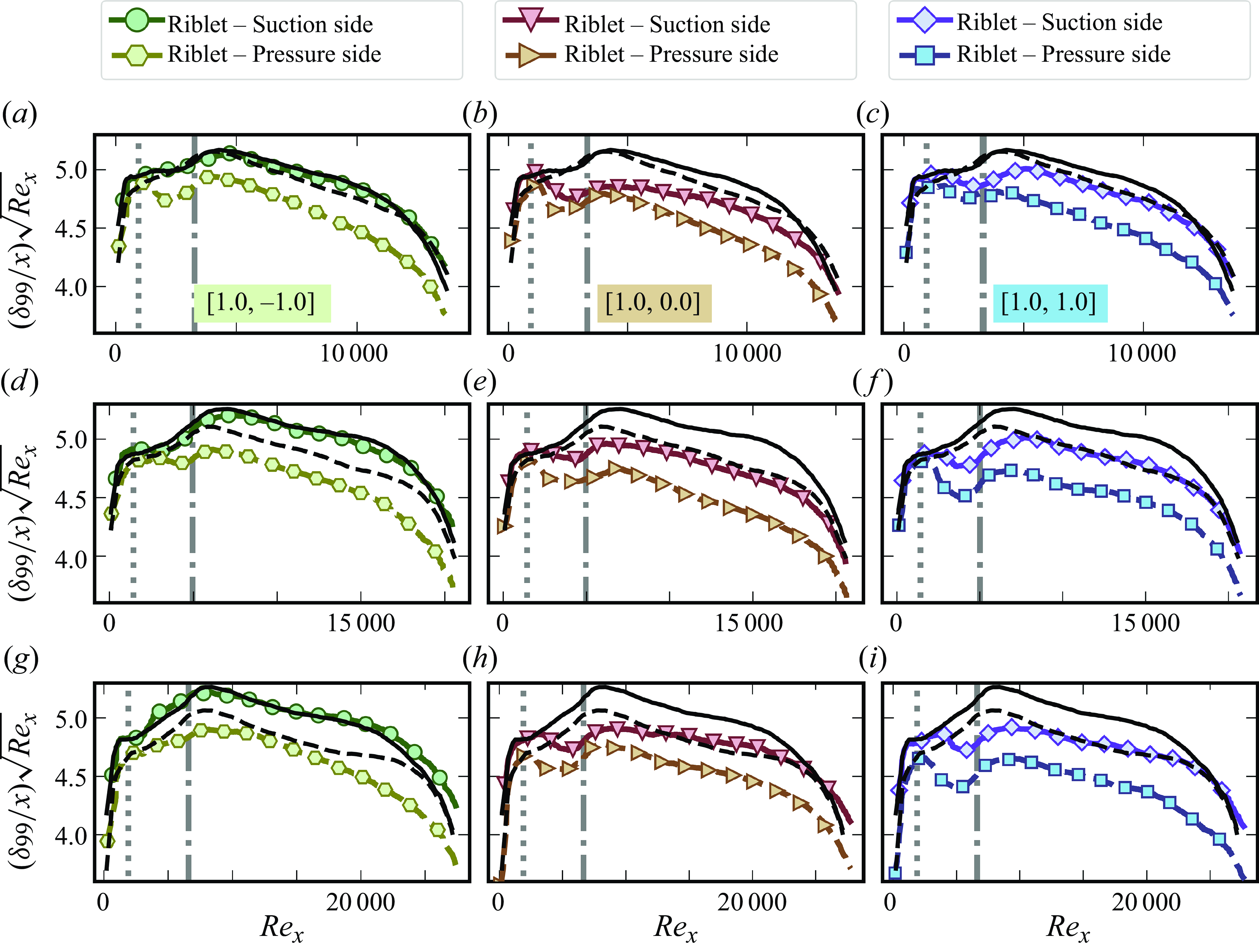
Figure 14. Distribution of the BL thickness, $\delta _{99}$
, normalised by local
$\delta _{99}$
, normalised by local $x/\sqrt {{ Re}_x}$
for all the riblet samples of
$x/\sqrt {{ Re}_x}$
for all the riblet samples of ${\mathcal {R}} = 1.0$
on the suction and pressure side for all tested Reynolds numbers. The
${\mathcal {R}} = 1.0$
on the suction and pressure side for all tested Reynolds numbers. The $\delta _{99}$
of the smooth reference on the suction and pressure side are shown with solid and dashed black lines, respectively. Locations of
$\delta _{99}$
of the smooth reference on the suction and pressure side are shown with solid and dashed black lines, respectively. Locations of $x_{{ LET}}$
and
$x_{{ LET}}$
and $x_{{ Flat}}$
are marked by grey dotted and dash-dotted vertical lines.
$x_{{ Flat}}$
are marked by grey dotted and dash-dotted vertical lines.
Lastly, this reduction in the overall thickness of the fictitious boundary of the sample and the BL seen by the outer inviscid flow can be a substantial help to samples that cannot capture a reduction in the frictional drag compared with the smooth surface. Example of that is the [1.0, 0.0] sample thatfrom a frictional point is not able to reduce the drag force, however, as seen in figure 9(b,e,h), with a large extent of the plate experiencing $m$
values larger than the smooth reference, the
$m$
values larger than the smooth reference, the $\delta _{99}$
of this sample experiences enough reduction on both sides, especially in the early part of the Flat region (see figure 14
b,e,h) to experience noticeable levels of pressure recovery (figure 13
d,e,f) at the trailing edge and ultimately becoming drag-reducing (figure 4).
$\delta _{99}$
of this sample experiences enough reduction on both sides, especially in the early part of the Flat region (see figure 14
b,e,h) to experience noticeable levels of pressure recovery (figure 13
d,e,f) at the trailing edge and ultimately becoming drag-reducing (figure 4).
4. Conclusions
Here, we evaluate the possibility of using riblets as a drag-reducing technique on a standalone, finite-sized slender body. We use a three-tiered measurement approach to capture the total drag force and decompose it into the frictional and pressure components. We further use the local shear stress and pressure and the distribution of the velocity profiles to explore the drag-changing performance of the riblets. We present a holistic view of the impact of the riblets on the flow around this body, showing both the positive and negative aspects of the use of this drag-reducing device on the total drag as well as components of the drag force. We show an intertwined relationship between the good and bad points presented, and believe the complex interactions between the BLs over riblets on the suction and pressure sides, the resulting pressure distribution, as well as the choice of the design of the riblets in leading and trailing edges are all important factors that researchers need to consider when designing and optimising riblets for finite-sized bodies especially in the higher-Reynolds-number ranges of the laminar regimes.
Overall, a majority of the cases presented here, operated in high-Reynolds-number laminar regimes, showed some level of drag reduction (total drag), with drag-increasing cases all having a convex riblet shape ( ${\kappa _2} = -{\mathcal {R}}$
). The largest total reduction is seen for the [1.0, 1.0] sample at
${\kappa _2} = -{\mathcal {R}}$
). The largest total reduction is seen for the [1.0, 1.0] sample at ${ Re}_{L} = 18\,500$
and
${ Re}_{L} = 18\,500$
and $24\,200$
with a
$24\,200$
with a $5.8\,\%\!-\!6.5\,\%$
reduction recorded. Owing to the finitesise of the sample, between
$5.8\,\%\!-\!6.5\,\%$
reduction recorded. Owing to the finitesise of the sample, between $42\,\%\!-\!52\,\%$
of the drag is due to the frictional component and around
$42\,\%\!-\!52\,\%$
of the drag is due to the frictional component and around $23\,\%\!-\!34\,\%$
due to the pressure, with the remaining
$23\,\%\!-\!34\,\%$
due to the pressure, with the remaining $20\,\%\!-\!24\,\%$
attributed to other effects that cannot be captured via planar PIV measurements. The contribution of the frictional drag to the total drag change is limited, and as the global Reynolds number is increased, more of the cases experienced a reduction in the
$20\,\%\!-\!24\,\%$
attributed to other effects that cannot be captured via planar PIV measurements. The contribution of the frictional drag to the total drag change is limited, and as the global Reynolds number is increased, more of the cases experienced a reduction in the $D_f$
. On the other hand, the contribution of the pressure drag to the reduction is more pronounced with most of the cases experiencing some level of reduction in the
$D_f$
. On the other hand, the contribution of the pressure drag to the reduction is more pronounced with most of the cases experiencing some level of reduction in the $D_p$
compared with the smooth reference.
$D_p$
compared with the smooth reference.
Further investigation of the localised shear stress distribution reveals a more complex behaviour that leads to the subpar performance of the riblets in terms of the frictional drag force. On the one hand, the asymmetry of the flow field, due to the angle of attack of the sample, results in an asymmetry in the contribution of the suction and pressure side of the sample to the $D_f$
. The suction sides of most samples are drag-reducing while the pressure sides tend to be drag-increasing. Thus, cumulatively, the increase of the pressure side counteracts the gains of the suction side. Only four of the cases (see figure 8) see frictional reductions on both sides. On the other hand, the presence of riblets gives rise to four different
$D_f$
. The suction sides of most samples are drag-reducing while the pressure sides tend to be drag-increasing. Thus, cumulatively, the increase of the pressure side counteracts the gains of the suction side. Only four of the cases (see figure 8) see frictional reductions on both sides. On the other hand, the presence of riblets gives rise to four different $\langle C_f \rangle (x)$
patterns (types I--IV). The pattern of type I is similar to that of the smooth reference, where with different rates compared with the smooth
$\langle C_f \rangle (x)$
patterns (types I--IV). The pattern of type I is similar to that of the smooth reference, where with different rates compared with the smooth $\langle C_f \rangle (x)$
, it takes a decreasing trend along the length. The patterns of types II--IV show clear differences leading to
$\langle C_f \rangle (x)$
, it takes a decreasing trend along the length. The patterns of types II--IV show clear differences leading to $\langle C_f \rangle (x)$
becoming either constant or increasing along the length of the sample. This results in a non-monotonic distribution of the
$\langle C_f \rangle (x)$
becoming either constant or increasing along the length of the sample. This results in a non-monotonic distribution of the $\unicode{x1D6E5} \langle \tau _{n=0} \rangle$
with the possibility of having regions of both
$\unicode{x1D6E5} \langle \tau _{n=0} \rangle$
with the possibility of having regions of both $\langle C_f \rangle (x) \gt C_{f,0}(x)$
and
$\langle C_f \rangle (x) \gt C_{f,0}(x)$
and $\langle C_f \rangle (x) \lt C_{f,0}(x)$
(i.e.
$\langle C_f \rangle (x) \lt C_{f,0}(x)$
(i.e. $\unicode{x1D6E5} \langle \tau _{n=0} \rangle \gt 0$
or
$\unicode{x1D6E5} \langle \tau _{n=0} \rangle \gt 0$
or $\unicode{x1D6E5} \langle \tau _{n=0} \rangle \lt 0$
) where again the reductions are counteracted by the increases, leading to the frictional drag integral capturing much less reduction in the frictional drag than the riblets’ local shear-reducing potential observed.
$\unicode{x1D6E5} \langle \tau _{n=0} \rangle \lt 0$
) where again the reductions are counteracted by the increases, leading to the frictional drag integral capturing much less reduction in the frictional drag than the riblets’ local shear-reducing potential observed.
With access to the $\langle C_f \rangle (x)$
distribution on both sides of the sample, we also decompose the drag into components within the leading edge (LE and LET) and Flat segments of the samples. We see that the choice of mimicking the shark nose in the design of the leading edge allows us to avoid large
$\langle C_f \rangle (x)$
distribution on both sides of the sample, we also decompose the drag into components within the leading edge (LE and LET) and Flat segments of the samples. We see that the choice of mimicking the shark nose in the design of the leading edge allows us to avoid large $\unicode{x1D6E5} \langle \tau _{n=0} \rangle$
values in that region, and the incremental growth of the riblets also guides the development of the velocity field and
$\unicode{x1D6E5} \langle \tau _{n=0} \rangle$
values in that region, and the incremental growth of the riblets also guides the development of the velocity field and $\langle C_f \rangle (x)$
in the LET region. In this design the
$\langle C_f \rangle (x)$
in the LET region. In this design the $\langle C_f \rangle (x)$
of the LE region is not available for modification.
$\langle C_f \rangle (x)$
of the LE region is not available for modification.
The impact of riblets on the flow field is mostly confined to the BL near the wall and we use this idea in our experimental procedure to measure the spanwise-averaged velocity field around the body using 2D-2C PIV. By fitting the velocity profiles locally to an updated form of the FS family of BL solutions, we find the parameters $m$
(capturing the effect of pressure gradient, streamwise and spanwise viscous diffusion, nonlinear terms due to spanwise averaging and curvature of the leading edge) and
$m$
(capturing the effect of pressure gradient, streamwise and spanwise viscous diffusion, nonlinear terms due to spanwise averaging and curvature of the leading edge) and $n_0$
(effective origin of the velocity profiles). We see similar repeated patterns in the distributions of
$n_0$
(effective origin of the velocity profiles). We see similar repeated patterns in the distributions of $m$
and
$m$
and $n_0$
, while the magnitudes of the two parameters show an intertwined relationship thatis driven by the flow dynamics and the available cross-sectional space inside the grooves. The distribution of
$n_0$
, while the magnitudes of the two parameters show an intertwined relationship thatis driven by the flow dynamics and the available cross-sectional space inside the grooves. The distribution of $n_0$
shows clear signs of flow retardation and the creation of layers of slow-moving fluid inside the grooves thatthen leads to the flow being pushed out of the grooves and the magnitude of the
$n_0$
shows clear signs of flow retardation and the creation of layers of slow-moving fluid inside the grooves thatthen leads to the flow being pushed out of the grooves and the magnitude of the $n_0$
decreasing prior to the trialing edge. This directly impacts the distribution of
$n_0$
decreasing prior to the trialing edge. This directly impacts the distribution of $m$
where after an initial decrease,
$m$
where after an initial decrease, $m$
takes an increasing trend in the second half of the plate, with rates faster than that of the smooth reference (as the flow is squeezed between the higher
$m$
takes an increasing trend in the second half of the plate, with rates faster than that of the smooth reference (as the flow is squeezed between the higher $n_0$
and the edge of the BL) and thus resulting in type II--IV shear distributions.
$n_0$
and the edge of the BL) and thus resulting in type II--IV shear distributions.
In addition, we use the distribution of $m$
alongside the distribution of the pressure gradient on a line parallel to the wall, in the form of the
$m$
alongside the distribution of the pressure gradient on a line parallel to the wall, in the form of the ${\mathcal {G}}$
, to explore the effect of the streamwise and spanwise viscous terms, nonlinear terms due to spanwise averaging and the curvature effects. While
${\mathcal {G}}$
, to explore the effect of the streamwise and spanwise viscous terms, nonlinear terms due to spanwise averaging and the curvature effects. While $m$
cannot distinguish between the order of magnitude of these terms, based on the physics, we estimate that the BL development along the grooves and inside the slow-moving fluid layer leads to recirculation regions as identified by
$m$
cannot distinguish between the order of magnitude of these terms, based on the physics, we estimate that the BL development along the grooves and inside the slow-moving fluid layer leads to recirculation regions as identified by ${\mathcal {G}}\gt 0$
regions. Overall, the similarity of the
${\mathcal {G}}\gt 0$
regions. Overall, the similarity of the ${\mathcal {G}}$
of the smooth and riblet surfaces gives us confidence that the effect of the spanwiseaveraging on the nonlinear terms are minimal and we can extract valuable information from planar PIV experiments for riblet surfaces.
${\mathcal {G}}$
of the smooth and riblet surfaces gives us confidence that the effect of the spanwiseaveraging on the nonlinear terms are minimal and we can extract valuable information from planar PIV experiments for riblet surfaces.
The impact of riblets on the near-wall BL is also evident in changes in the location of the edge of the BL as seen by the inviscid outer flow. The cross-sectional space available inside the grooves and the distribution of $m$
along the side of the samples leads to, on average, thinner BLs compared with the smooth reference, especially on the pressure sides of the samples. This results in a pressure recovery seen in the trailing edge of most of the riblet samples and, thus, clear reductions in the pressure drag compared with the smooth reference. This not only helps the samples that were
$m$
along the side of the samples leads to, on average, thinner BLs compared with the smooth reference, especially on the pressure sides of the samples. This results in a pressure recovery seen in the trailing edge of most of the riblet samples and, thus, clear reductions in the pressure drag compared with the smooth reference. This not only helps the samples that were $D_f$
-reducing, but makes it possible for a few of the
$D_f$
-reducing, but makes it possible for a few of the $D_f$
-increasing samples to become cumulatively drag-reducing when the pressure component is added.
$D_f$
-increasing samples to become cumulatively drag-reducing when the pressure component is added.
Overall, the evidence presented supports the idea that the implementation of riblets for reducing the drag on finite-sized, standalone samples is feasible. However, to gain the most benefit from this approach, it requires a more comprehensive design plan that considers the effect of the friction and pressure drags simultaneously. While in the ideal design, the riblets on both sides follow a type I $\langle C_f \rangle (x)$
distribution along the length, are cumulatively
$\langle C_f \rangle (x)$
distribution along the length, are cumulatively $D_f$
-reducing, and the edges of the BL are sufficiently adjusted for the
$D_f$
-reducing, and the edges of the BL are sufficiently adjusted for the $D_p$
to also be reduced, there are a variety of ways where the riblet design can be optimised to enhance the reduction in either
$D_p$
to also be reduced, there are a variety of ways where the riblet design can be optimised to enhance the reduction in either $D_f$
or
$D_f$
or $D_p$
to achieve desired levels of reductions. The leading and trailing edges of the body play important roles in guiding the development of the
$D_p$
to achieve desired levels of reductions. The leading and trailing edges of the body play important roles in guiding the development of the $\langle C_f \rangle (x)$
along the length of the sample and potential adjustments to the curvature of those regions could improve the performance of the riblets as shear-reducing agents. In addition, the reduction in the pressure component of the drag due to the adjustment in the BL thickness opens up another avenue for riblets to also be considered for bulkier vehicles that experience a larger contribution from the pressure drag.
$\langle C_f \rangle (x)$
along the length of the sample and potential adjustments to the curvature of those regions could improve the performance of the riblets as shear-reducing agents. In addition, the reduction in the pressure component of the drag due to the adjustment in the BL thickness opens up another avenue for riblets to also be considered for bulkier vehicles that experience a larger contribution from the pressure drag.
With a planar PIV measurement, we have been able to capture the local flow behaviour using spanwise-averaged measures as well as cumulative integral measures. However, there is still a need for an even more localised approach to capture the spanwise details of the flow field both inside and outside the grooves. Future experimental and numerical efforts need to be used to evaluate nuances that are only captured in a full three-dimensional view of the flow field and whether there can be added benefits to acquisition of the added data. Capturing the full three-dimensional flow field inside the grooves will allow us to further explore the effect of the shape of the riblets on their ability to reduce the drag force and pave the way for additional localised optimisation efforts focused on the shape of the riblets. Further modelling efforts supported by numerical simulations or stereo- or tomo-PIV efforts focused on the characterisation of the flow inside the grooves can be used to add additional validation to the spanwise-averaging method presented here and improve our predictive capability. In addition, extensions of this work to larger Reynolds numbers, turbulent flows, as well as those with non-constant pressure distributions will be instrumental in expanding the use of drag-reducing riblets to smaller and bulkier vehicles and bluff bodies as well.
The evidence from this research opens the way for future studies to focus more on the local changes that the pressure coefficient can experience due to imposed passive or active drag reduction devices. While no changes were observed in the $C_f$
in the LE area, we notice slight alterations in the distribution of the pressure coefficient prior to the start of the riblets in the LE region as well as differences in the riblet-covered regions. In addition, in a recent work, using travelling waves for drag reduction, Quadrio et al. (Reference Quadrio, Chiarini, Banchetti, Gatti, Memmolo and Pirozzoli2022) report a similar trend where the distribution of the pressure coefficient is changed upstream of the location of the imposed control. The possibility of such changes in the pressure coefficient can have implications for strategic ways of altering the lift force via drag-reduction techniques and should be further explored for lift-generating bodies and situations, including larger angles of attack. The limitations of the current set-up stops us from finetuning the angles of attack of the bodies to sub-degree accuracy and need to calculate the final values after the completion of each measurement campaign. Future expansions should also consider enhancing the experimental set-up to increase the accuracy of the sample installation to reduce the variations in the final angles of attack of the samples.
$C_f$
in the LE area, we notice slight alterations in the distribution of the pressure coefficient prior to the start of the riblets in the LE region as well as differences in the riblet-covered regions. In addition, in a recent work, using travelling waves for drag reduction, Quadrio et al. (Reference Quadrio, Chiarini, Banchetti, Gatti, Memmolo and Pirozzoli2022) report a similar trend where the distribution of the pressure coefficient is changed upstream of the location of the imposed control. The possibility of such changes in the pressure coefficient can have implications for strategic ways of altering the lift force via drag-reduction techniques and should be further explored for lift-generating bodies and situations, including larger angles of attack. The limitations of the current set-up stops us from finetuning the angles of attack of the bodies to sub-degree accuracy and need to calculate the final values after the completion of each measurement campaign. Future expansions should also consider enhancing the experimental set-up to increase the accuracy of the sample installation to reduce the variations in the final angles of attack of the samples.
Future efforts should also include time-resolved measurements to capture the unsteady flow dynamics past the trailing edge of finite aspect ratio bodies, and to evaluate how the combination of the riblets and the geometry of the body, especially the length and aspect ratio, affect the flow bifurcations, instabilities and vortex shedding patterns. Such time-resolved efforts should also be extended to bodies at larger angles of attack that better reflect the situation of a small ‘air/waterborne vehicle.’
Supplementary material
Supplementary material is available at https://doi.org/10.1017/jfm.2025.10185.
Acknowledgements
The optical profilometry has been performed at the Harvard University Center for Nanoscale Systems (CNS); a member of the National Nanotechnology Coordinated Infrastructure Network (NNCI), which is supported by the National Science Foundation under NSF award no. ECCS-2025158. The authors would like to thank Dr Prasoon Suchandra for helpful discussions.
Funding
This research has been supported by the Rowland Fellows program at Harvard University.
Declaration of interests
The authors report no conflict of interest.
Data availability statement
The raw data that support the findings of this study are available from the corresponding author upon reasonable request.
Author contributions
S.F.: investigation, formal analysis, visualisation, writing (original draft), writing (review andediting). S.R.: conceptualisation, methodology, formal analysis, software, visualisation, writing (original draft), writing (review and editing), supervision, funding acquisition.


 Open access