


1. Introduction
The study of stratified flows has attracted considerable attention over the past few decades due to their importance in many environmental and industrial processes. In the oceans, stratification occurs due to differences in salinity and/or temperature, leading to mostly stably stratified flows. Turbulence in these flows plays a significant role in the transport of momentum and mass and is crucial in shaping the global climate (Linden Reference Linden1979; Riley & Lelong Reference Riley and Lelong2000; Gregg et al. Reference Gregg, D'Asaro, Riley and Kunze2018; Caulfield Reference Caulfield2020). An interesting open question concerns the maintenance of turbulence and its associated irreversible turbulent mixing under strong stable stratification, which tends to suppress turbulence.
When stratification is relatively weak, stably stratified flows can be linearly unstable. It is well known that linear shear instabilities, such as the Kelvin–Helmholtz instability (KHI) (Hazel Reference Hazel1972; Smyth, Klaassen & Peltier Reference Smyth, Klaassen and Peltier1988) and Holmboe wave instability (HWI) (Holmboe Reference Holmboe1962), can cause transition of a laminar stratified flow to turbulence, inducing strong mass and momentum transport (Caulfield Reference Caulfield2021). Over the past 50 years, numerous studies have been carried out to understand these instabilities and their relation to mixing (Thorpe Reference Thorpe1968; Smyth et al. Reference Smyth, Klaassen and Peltier1988; Carpenter et al. Reference Carpenter, Tedford, Rahmani and Lawrence2010b; Salehipour, Peltier & Mashayek Reference Salehipour, Peltier and Mashayek2015; Zhou et al. Reference Zhou, Taylor, Caulfield and Linden2017). In most of these studies, the density isopycnals are perpendicular to the direction of gravity, which does not explicitly drive the flows.
However, in many natural systems, density isopycnals are not exactly perpendicular to gravity, in which case non-zero streamwise gravity forces come into play and may partially drive the flow. One notable example is the internal tide interacting with the sloping bottom topography of the oceanic continental shelf (Garrett & Kunze Reference Garrett and Kunze2007). At a critical slope, the internal tide provides an additional energy production pathway that leads to turbulent mixing of temperature, salinity and other tracers (Gayen & Sarkar Reference Gayen and Sarkar2010). Similarly, many engineering flows occur along an inclined boundary. Examples can be found in building ventilation systems (Linden Reference Linden1999), where indoor/outdoor air is often exchanged through inclined ventilation ducts, producing mixing and dispersion of heat and indoor pollutants. In gas-cooled nuclear reactors, a failure of a cooling duct will result in a turbulent exchange flow between the carbon dioxide inside and the outside air, which is critical to the modelling of depressurisation accidents (Leach & Thompson Reference Leach and Thompson1975; Mercer & Thompson Reference Mercer and Thompson1975).
Studies on the influence of longitudinal gravitational forcing on the onset of turbulence in stratified exchange flows remain limited. One notable recent body of work is the stratified inclined duct (SID) experiment (Meyer & Linden Reference Meyer and Linden2014; Lefauve, Partridge & Linden Reference Lefauve, Partridge and Linden2019; Lefauve & Linden Reference Lefauve and Linden2020). These studies investigated the transition and turbulent mixing of the exchange flow in an inclined duct that connected two reservoirs with fluids at different densities or temperatures. To understand the mechanism of transition in SID, Lefauve et al. (Reference Lefauve, Partridge, Zhou, Dalziel, Caulfield and Linden2018) conducted a linear stability analysis (LSA) using a base state extracted from the SID experiment. Subsequently, Ducimetière et al. (Reference Ducimetière, Gallaire, Lefauve and Caulfield2021) systematically investigated the three-dimensional (3-D) unstable modes in inclined ducts, focusing on the effects of sidewall confinement. These studies focused primarily on HWI (and secondarily on KHI), which have wavelengths comparable to the thickness of the shear layers. Interestingly, Ducimetière et al. (Reference Ducimetière, Gallaire, Lefauve and Caulfield2021) observed a secondary instability at significantly longer wavelengths than KHI and HWI and attributed it to the effect of the tilt angle. Recently, Atoufi et al. (Reference Atoufi, Zhu, Lefauve, Taylor, Kerswell, Dalziel, Lawrence and Linden2023) studied the mechanism of transition by applying shallow water equations as a diagnostic tool to analyse a new numerical simulation database of SID (Zhu et al. Reference Zhu, Atoufi, Lefauve, Taylor, Kerswell, Dalziel, Lawrence and Linden2023a). They suggested that the instability of long shallow water waves (i.e. a long-wave KHI in the presence of top and bottom solid boundaries) may cause turbulence in the SID. Although the longitudinal gravitational forcing was included in the numerical simulation data, it was not included explicitly in the shallow water model.
In this paper, we explore explicitly the impact of longitudinal gravitational forces on the instability of long waves and on potential new pathways towards turbulence, restricting ourselves to a two-dimensional (2-D) geometry. In § 3, we examine the linear instabilities in inclined channels and conduct a thorough exploration of the parameter space. We identify three new families of long-wave instabilities distinct from the well-known HWI and KHI, and map in parameter space these long-wave instabilities that dominate the flow. In § 4, we then investigate the evolution of these new instabilities by conducting 2-D forced direct numerical simulations (DNS), and discuss their impact on turbulence and energy transfers. Finally, we conclude in § 5.
2. Methodology
2.1. Problem formulation and governing equations
In this section, we present the equations required for LSA of a stratified exchange flow between two fluid layers having density  $\rho _0 \pm \Delta \rho /2$ (where $\rho _0$ is the reference density and $0<\Delta \rho \ll \rho _0$ is the density difference) in a 2-D stratified inclined channel (SIC, see figure 1a). Following the SID experimental literature, lengths are non-dimensionalised by the half-channel height $H^*$, velocity by the buoyancy-velocity scale $U^* \equiv \sqrt {g^\prime H^*}$ (where $g^\prime =g\Delta \rho /\rho _0$ is the reduced gravity), time by the advective time unit $H^*/U^*$, pressure by $\rho _0 U^{*2}$ and density variations around $\rho _0$ by $\Delta \rho /2$, respectively. The non-dimensional continuity, Navier–Stokes and scalar equations under the Boussinesq approximation are
 \begin{gather} \boldsymbol{\nabla} \boldsymbol{\cdot} \boldsymbol{u} = 0, \end{gather}
 \begin{gather}\frac{\partial \boldsymbol{u}}{\partial t}+\boldsymbol{u}\boldsymbol{\cdot} \boldsymbol{\nabla}\boldsymbol{u} ={-} \boldsymbol{\nabla}p + \frac{1}{Re} \nabla^{2}\boldsymbol{u} + {Ri} \rho \boldsymbol{\hat{g}}, \end{gather}
 \begin{gather}\frac{\partial \rho}{\partial t}+\boldsymbol{u}\boldsymbol{\cdot} \boldsymbol{\nabla}\rho = \frac{1}{{{\textit{Re}}\, {\textit{Pr}}}} \nabla^{2}\rho, \end{gather}
where  $\boldsymbol {u}=(u,v,w)$ is the non-dimensional velocity in the 3-D coordinate system $\boldsymbol {x}=(x,y,z)$, where the $x$,
$x$,  $y$,
$y$,  $z$ axes are the longitudinal, spanwise and wall-normal direction of the channel, respectively. In this coordinate system gravity $\boldsymbol {g}$ is pointing downwards at a angle $\theta$ to the $-z$ axis, i.e. $\boldsymbol {g}=g \boldsymbol {\hat {g}}=g[\sin {\theta }, 0, -\cos {\theta }]$, and $p$ and $\rho$ are the non-dimensional pressure and density, respectively. The dimensionless parameters are the Reynolds number Re $\equiv H^*U^*/\nu$ ( $\nu$ is the kinematic viscosity), the Prandtl number ${\textit {Pr}}\equiv \nu /\kappa$ ( $\kappa$ is the scalar diffusivity) and Richardson number ${\textit {Ri}} \equiv g^\prime H^\ast /(2U^{\ast })^2=1/4$ (fixed here because of the buoyancy velocity scale).

Figure 1. (a) Schematic of the 2-D shear flow in a stratified channel inclined at an angle  $\theta$, and (b) base velocity $U(z)$, density $R(z)$ and corresponding background gradient Richardson number $Ri_b(z)\equiv Ri({\rm d}R/{\rm d}z)/({\rm d} U/{\rm d} z)^2$ profiles computed from (2.10) and (2.11).
2.2. Formulation of LSA
We now apply a LSA (Drazin & Reid Reference Drazin and Reid2004; Smyth & Carpenter Reference Smyth and Carpenter2019) to the SIC. Lefauve et al. (Reference Lefauve, Partridge, Zhou, Dalziel, Caulfield and Linden2018) and Ducimetière et al. (Reference Ducimetière, Gallaire, Lefauve and Caulfield2021) have shown that the fastest-growing mode is 2-D so we impose infinitesimal 2-D perturbations to a one-dimensional base state. The velocity, density and pressure fields are thus decomposed as
 \begin{gather} \boldsymbol{u}=\boldsymbol{U}+\boldsymbol{u}^\prime=[U(z),0,0]+[u^\prime,0,w^\prime], \end{gather}
 \begin{gather}p = P(z)+p^\prime, \end{gather}
 \begin{gather}\rho = R(z) +\rho^\prime, \end{gather}
where capital letters and superscript primes represent the mean and perturbation components of quantities, respectively. A normal mode perturbation of the form
 \begin{equation} \phi'(x,z,t) = \hat{\phi}(z)\exp{({\rm i}kx+\eta t)}, \end{equation}
is adopted. The base flows are obtained by solving for the numerical solution of the laminar exchange flow following Thorpe (Reference Thorpe1968), which will be introduced in § 2.3. Substituting (2.4)–(2.6) into (2.1)–(2.3) and linearising yields the same system as in Lefauve et al. (Reference Lefauve, Partridge, Zhou, Dalziel, Caulfield and Linden2018), i.e.
 \begin{equation} \eta \left[\begin{array}{cc} \Delta & \boldsymbol{\mathsf{0}} \\ \boldsymbol{\mathsf{0}} & \boldsymbol{\mathsf{I}} \end{array}\right] \left[\begin{array}{c} \hat{w} \\ \hat{\rho} \end{array}\right]=\left[\begin{array}{cc} \mathcal{L}_{ww} & \mathcal{L}_{w \rho} \\ \mathcal{L}_{\rho w} & \mathcal{L}_{\rho \rho} \end{array}\right] \left[\begin{array}{c} \hat{w} \\ \hat{\rho} \end{array}\right] , \end{equation}
where  $\boldsymbol{\mathsf{0}}$ and $\boldsymbol{\mathsf{I}}$ are the zero and identity matrices, respectively, and
 \begin{equation} \left. \begin{aligned} \mathcal{L}_{ww} & ={-}\mathrm{i}k U \Delta + \mathrm{i}k \mathscr{D}^2 U + {\textit{Re}}^{{-}1} \varDelta^2,\\ \mathcal{L}_{w \rho} & =Ri \left(k^2 \cos{\theta} -\mathrm{i} k \sin{\theta} \mathscr{D} \right), \\ \mathcal{L}_{\rho w} & ={-}\mathscr{D}R, \\ \mathcal{L}_{\rho \rho} & ={-}\mathrm{i} k U + \left({\textit{Re}} \, {\textit{Pr}} \right)^{{-}1} \Delta, \end{aligned} \right\} \end{equation}
where  $\varDelta =\mathscr {D}^2-k^2$ (the operator $\mathscr {D}=\partial /\partial z$ and $\mathscr {D}^2=\partial ^2/\partial z^2$). At the top and bottom boundaries ( $z=\pm 1$), no-slip and no-flux boundary conditions are applied for velocity and density, respectively. We also demonstrate the negligible effect of choosing a free-slip boundary condition for velocity in the Appendix A. To obtain the unstable modes, we solve the linear system (2.8) numerically using a second-order finite-difference discretisation described in Smyth & Carpenter (Reference Smyth and Carpenter2019). The spatial resolution is chosen based on the sharpness of the interface and is $(150, 150, 250, 400)$ grid points for ${\textit {Pr}}=(1$, $7$,
$7$,  $28$,
$28$,  $70)$, respectively (a sensitivity analysis for resolution ensured the convergence of the LSA results).
2.3. Base flows
The base state for density in our exchange flow is taken as a hyperbolic tangent (figure 1b)
 \begin{equation} R(z)={-}\tanh(z/\delta)={-}\tanh(2\sqrt{{\textit{Pr}}} \,z). \end{equation}
The interfacial thickness is  $\delta = 1/(2\sqrt {{\textit {Pr}}})$ to approximate the effect of diffusion (Smyth & Peltier Reference Smyth and Peltier1991). This empirical relation of ${\textit {Pr}}$ to the interfacial thickness is based on experimental and numerical observation of SID (Lefauve et al. Reference Lefauve, Partridge, Zhou, Dalziel, Caulfield and Linden2018; Zhu et al. Reference Zhu, Atoufi, Lefauve, Taylor, Kerswell, Dalziel, Lawrence and Linden2023a). The typical model (e.g. Smyth et al. Reference Smyth, Klaassen and Peltier1988) considers a shear layer driven by an arbitrary, controllable background shear. A similar procedure is applied to our SIC by modifying the laminar solution developed by Thorpe (Reference Thorpe1968) and imposing a background body force $\mathcal {F}=-\gamma {\textit {Ri}} R(z)$ (where $\gamma$ is a variable to control the magnitude of the force). This decouples the base velocity from the slope in SIC, allowing for the exploration of the $U-\theta$ space, as if being influenced by arbitrary external tidal forces or pressure gradients. The mean velocity profile $U(z)$ of the steady laminar exchange flow is obtained by integrating the 2-D momentum equation
 \begin{equation} {-}\frac{\partial P}{\partial x}+Ri R\sin{\theta} + \frac{1}{{\textit{Re}}} \frac{\partial ^2 U}{\partial z^2}+\mathcal{F}=0, \end{equation}
where  $-\partial P/\partial x= 0$ to satisfy the zero-flux condition of SIC. This yields the following laminar base state for the forced SIC:
 \begin{equation} U(z) ={-} {\textit{Re}} \, {\textit{Ri}} (\sin{\theta}-\gamma)I(z)+c_1 z+c_2, \end{equation}
where
 \begin{equation} I(z;{\textit{Pr}})=\frac{z^2}{2}+\ln{2} \delta z + \dfrac{\delta^2\operatorname{Li}_2\left(-\mathrm{e}^{2 z/\delta}\right)}{2}, \end{equation}
where  $\operatorname {Li}_2$ is the polylogarithm function of order two. The constants $c_1$ and $c_2$ are computed given the no-slip boundary condition at the walls $U(z=\pm 1)=0$ and are
 \begin{gather} c_1 = \tfrac{1}{2} {\textit{Re}} \, {\textit{Ri}} (\sin{\theta}-\gamma) \left[I(1)-I({-}1)\right], \end{gather}
 \begin{gather}c_2 = \tfrac{1}{2} {\textit{Re}} \, {\textit{Ri}} (\sin{\theta}-\gamma) \left[I(1)+I({-}1)\right]. \end{gather}
This solution  $U(z)$ is sinusoidal-like (figure 1b), much like those observed in experiments and simulations (Lefauve et al. Reference Lefauve, Partridge, Zhou, Dalziel, Caulfield and Linden2018; Zhu et al. Reference Zhu, Atoufi, Lefauve, Taylor, Kerswell, Dalziel, Lawrence and Linden2023a). The magnitude of the base velocity depends on ${\textit {Re}}$, $\theta$ and $\gamma$, while the shape depends more on $\delta$. In addition to the base state described by (2.12), we also conducted a LSA with a $\tanh$-shape velocity profile in Appendix A, to compare with the standard stratified free-shear layer model (Smyth et al. Reference Smyth, Klaassen and Peltier1988). These results were qualitatively consistent with those in the remainder of the paper, in terms of the existence of the same long- and short-wave families in SIC, suggesting the robustness of our results under broader flow conditions. A comprehensive investigation of the effects of background profiles is beyond the scope of this paper.
3. Results: new families of linear instabilities in SIC
Here we present the results from the LSA of SIC. We explore the parameter space of  $\theta -\gamma$ and map out three new families of long-wave instabilities in addition to the well-known short-wave HWI and KHI. We also investigate the impacts of ${\textit {Re}}$ and ${\textit {Pr}}$ in order to further understand the importance of these newly discovered long waves in the laminar–turbulent transition.
3.1. Five families of instabilities
We first fix  $({\textit {Re}},{\textit {Pr}},{Ri})=(1000,7,0.25)$ and vary the slope $\theta$ from $-10^{\circ }$ to $10^{\circ }$. When $\theta >0$, the SIC slopes downwards. In this configuration, streamwise gravity energises the mean flow, and vice versa when $\theta <0$. We vary the forcing factor $\gamma$, on which two important physical quantities depend: the interfacial background Richardson number $Ri_b$, defined as the gradient Richardson number of the background flow at the density interface $z=0$, i.e.
 \begin{equation} \left. Ri_b\equiv Ri\frac{{\rm d} R/{\rm d} z}{({\rm d} U/{\rm d} z)^2}\right|_{z=0}; \end{equation}
and the mass flux (or flow rate of buoyancy), which is given by
 \begin{equation} Q_m \equiv \tfrac{1}{2}\int_{{-}1}^1 \, R U \, {\rm d}z. \end{equation}
The Richardson number  $Ri_b$ is an important measure of the relative importance of stratification compared with shear, which is critical for stratified shear flow stability (Caulfield Reference Caulfield2020). The mass flux $Q_m$ is closely associated with the hydraulic control of exchange flows; a threshold value of $Q_m\approx 0.5$ indicates the existence of an internal hydraulic jump (Meyer & Linden Reference Meyer and Linden2014; Lefauve et al. Reference Lefauve, Partridge and Linden2019) which Atoufi et al. (Reference Atoufi, Zhu, Lefauve, Taylor, Kerswell, Dalziel, Lawrence and Linden2023) demonstrated to be equivalent to a relatively long KHI (requiring the existence of top and bottom boundaries). Note that, in accordance with the definition of the base state (featuring asymmetric $R$ and $U$ relative to $z=0$), the condition $Q_m=0$ implies $U(y)=0$.
Figure 2(a,c) shows the distribution of the growth rate  $\eta _r$ and wave frequency $\eta _i$ (and phase speed $c=-\eta _i/k$) of the fastest-growing modes in the parameter spaces ( $\theta, Ri_b$) and ( $\theta, Q_m$), respectively. Note that $\eta _r$ and $\eta _i$ are the real and imaginary components of the eigenvalues of the linear system (2.8). Examining the contour lines reveals five distinct families of unstable modes, shown schematically in figure 2(b,d). To better understand these modes, we show the dispersion relation of five representative cases (marked by the symbols in figure 2) dominated by the five families of instabilities in figure 3. Notably, two of these unstable modes, namely the HWI and KHI, can be triggered without the presence of a slope ( $\theta =0$, see vertical dotted black line). The other three families of modes rely on the presence of a slope ( $\theta \neq 0$) and are named long-wave instability (LWI), downslope very long-wave instability (DVLWI) and upslope very long-wave instability (UVLWI) based on their longer wavelengths ( $O(10\sim 10^{4})$) compared with the ‘short’ HWI and KHI ( $O(10^{-1}\sim 10)$). To the best of our knowledge, these unstable modes have not previously been reported in the literature.

Figure 2. Parameter space projections of the fastest growing mode: (a) the growth rate  $\eta _r$ (colours) and wave frequency $\eta _i$ (lines); (b) mode type, both in the $Ri_b-\theta$ parameter space; (c) the growth rate $\eta _r$ and wave frequency $\eta _i$; and (d) mode type, both in the $Q_m-\theta$ parameter space. Markers represent the five cases I,…, V in table 1 for which the fastest growing mode is calculated. Black solid lines are the natural convective ‘Thorpe’ base state (i.e. $\mathcal {F}=0$), and the horizontal dotted lines in (a,b) correspond to $Ri_b = 0.25.$

Figure 3. Dispersion relations for typical cases from figure 2: (a) positive growth rate  $\eta _r$ versus wavenumber $k$; and (b) positive growth rate $\eta _r$ versus wave frequency $\eta _i$.
Table 1. Numerical parameter values used for the DNS runs.

We find that the features of these instabilities are generally insensitive to the shapes of base profile and boundary conditions, despite adopting a base profile (2.12) and no-slip boundary in this section. To support this, we show in the Appendix A that these instabilities are found using a  $\tanh$-shape base state and free-slip boundary condition, as used by Smyth & Winters (Reference Smyth and Winters2003). This suggests that these instabilities can exist in a wide range of stratified exchange flows along a slope. In the following sections, we characterise the five families of unstable modes in more detail.
3.1.1. Holmboe wave instability
The HWI (Holmboe Reference Holmboe1962) occurs when the density interface is thinner than the shear layer and results from the resonance between vorticity waves at the edges of the shear layer and internal gravity waves at the density interface (Caulfield Reference Caulfield1994; Carpenter et al. Reference Carpenter, Tedford, Rahmani and Lawrence2010b). It gives rise to a pair of counter-propagating growing modes on either side of the density interface.
In SIC, the regime dominated by HWI exists from  $\theta =-10^\circ$ to $2^\circ$ and $Ri_b=0.3$ to $4$ (
$4$ ( $Q_m=0.1$ to $0.3$) in figure 2. The dispersion relation of HWI is shown in figure 3, where HWI has a pair of complex conjugate eigenvalues with non-zero phase speed $c=-\eta _i/k$. It is well known that horizontal stratified shear flows can become unstable at $Ri_b>0.25$ given a base flow with sufficiently large thickness ratio between the shear layer and density layers (Smyth et al. Reference Smyth, Klaassen and Peltier1988; Alexakis Reference Alexakis2009), leading to HWI. In this scenario, the minimum gradient Richardson number $\min (Ri_g(z))<0.25\leq Ri_b$, and the Miles–Howard criterion (Howard Reference Howard1961; Miles Reference Miles1961), which, strictly speaking, is intended for steady, inviscid Boussinesq flows, can still be applied to $Ri_g(z)$ (Smyth et al. Reference Smyth, Klaassen and Peltier1988; Caulfield Reference Caulfield2021). In figure 2, HWI can sustain at $Ri_b\sim 10$. We also notice that HWI can be induced over a wide range of $\theta$. The HWI-dominated regime gradually shrinks from $\theta <0$ to $\theta \approx 2^\circ$. This indicates that increasing downward slopes have a damping effect on HWI, a phenomenon that has not been previously discussed in the literature and constitutes a new result.
3.1.2. Kelvin–Helmholtz instability
The KHI arises due to the interaction of vorticity waves at two edges of finite shear layers, leading to a sequence of stationary vortex billows that roll up the denser fluids and cause significant mixing (Hazel Reference Hazel1972; Smyth & Peltier Reference Smyth and Peltier1991; Carpenter et al. Reference Carpenter, Tedford, Heifetz and Lawrence2011). However, unlike these previous studies (with the exception of the recent studies (Atoufi et al. Reference Atoufi, Zhu, Lefauve, Taylor, Kerswell, Dalziel, Lawrence and Linden2023; Liu, Kaminski & Smyth Reference Liu, Kaminski and Smyth2023)) the KHI observed here in the SIC geometry is bounded by no-slip solid boundaries at  $z=\pm 1$.
In SIC, KHI has a zero phase speed and a characteristic wavelength of  ${\rm \pi}$, consistent with previous studies by Smyth & Carpenter (Reference Smyth and Carpenter2019), Caulfield (Reference Caulfield2021) and Smyth & Peltier (Reference Smyth and Peltier1991). The KHI dominates the flow at small $Ri_b\lesssim 0.25$, in agreement with the Miles–Howard criterion. Interestingly, like HWI, the longitudinal gravity force can affect the regimes of KHI. The upper bound of the KHI-dominant regime in figure 2(a) increases linearly from $Ri_b=0.15$ to $0.25$ as $\theta$ increases from $-10^\circ$ to $10^\circ$. This suggests an enhancement of KHI by a downward slope, which we believe to be an additional new result.
3.1.3. Long-wave instability
Of the three new instabilities that arise with slopes, the LWI dominates the flow at large downward slopes ( $\theta >4^\circ$) and a weak shear (strong stratification). In contrast to KHI and HWI, the LWI has a longer wavelength ( $O(10- 10^{2})$). Note that the LWI discussed in this paper is distinct from the long waves supported by shallow-water (hydraulic) theory (Lawrence Reference Lawrence1990; Atoufi et al. Reference Atoufi, Zhu, Lefauve, Taylor, Kerswell, Dalziel, Lawrence and Linden2023) which are essentially Kelvin–Helmholtz (KH) waves with a large $k$ (satisfying the hydrostatic approximation) and which can exist at $\theta =0$. The LWI, on the other hand, specifically requires $\theta \neq 0$. As depicted in figure 3, its phase speed is near-zero. This instability can be triggered at $Ri_b\gg 1$, at which the shear-induced HWI and KHI vanish. Note that the presence of a mean shear can affect LWI by modifying its growth rate and phase speed. In terms of wave interaction, since vorticity waves vanish as $Q_m\rightarrow 0$, we hypothesise that LWI is a result of the interaction between gravity waves at the density interface and the streamwise gravity force. We will delve into this aspect in greater detail in § 3.3. We also note that the $Q_m=0$ condition may be arbitrary when subjected to a non-zero slope, as it requires the gravity and pressure forces to be precisely cancelled by external body forces $\mathcal {F}$ in (2.11). In practice, such a precisely balanced condition is expected to be rarely observed.
3.1.4. Downslope very long-wave instability
The new DVLWI shares similarities with the LWI, in that it can exist at weak shear (strong stratification) and has a long wavelength. However, DVLWI dominates the flow under different conditions, namely when  $2^\circ <\theta <5^\circ$ and $Ri_b>0.25$ ( $Q_m<0.5$). It is also characterised by very long wavelengths of $O(10^{2}- 10^{3})$ (wavenumbers $k=O(10^{-3})\sim O(10^{-2})$) and, interestingly, a pair of eigenmodes with complex conjugate phase speeds (figure 3). As with the HWI, we thus expect a pair of unstable DVLWI modes propagating with opposite phase speeds. The evolution of these unstable long waves and their connections to the onset of turbulence will be further discussed in § 4.
3.1.5. Upslope very long-wave instability
For  $\theta<0$, i.e. for upward slopes, another type of very long-wave instability (UVLWI) appears with wavelengths $\geq 10^2$ (wavenumbers $k< O(10^{-2})$) and a zero phase speed (figure 3). This instability is similar to LWI and DVLWI in that it requires a slope ( $\theta \neq 0$) and can exist in a strongly stratified environment. Contrary to the usually significantly smaller growth rate of the long waves compared with the corresponding short waves, the UVLWI has in fact a comparable growth rate as HWI; this will be further discussed in § 3.5.
Importantly, these long-wave instabilities have the potential to trigger and sustain turbulence in strongly stable stratified flows, which are a priori regarded as stable. In § 4 we will show that these new instabilities can indeed destabilise the flow at  $Ri_b > 1$, eventually resulting in nonlinear bursting and a transition to turbulence and mixing. It is also important to note that figure 2 only shows the fastest growing modes, whereas multiple families of instabilities can coexist in certain regions, as shown in figure 3. As a result, the regions of instability overlap, and the neutral boundary of each instability cannot be identified from figure 2. In § 3.5, we will address this challenge by introducing an unsupervised clustering technique to isolate the neutral boundary of each family. Furthermore, in figure 2, we include a black line computed from $\gamma =0$, i.e. the natural convective ‘Thorpe’ base state with forcing $\mathcal {F}=0$. Under the parameters discussed so far ( ${\textit {Re}}=1000$, ${\textit {Pr}}=7$), this line does not intersect any long-wave instabilities in parameter space. Nonetheless, it is important to note that different ${\textit {Re}}$ and ${\textit {Pr}}$ or boundary conditions can modify the regimes of the long-wave instability and interact with the base flow. An example is demonstrated in § 3.6 for ${\textit {Pr}}=28$.
3.2. Link between long- and short-wave instabilities
In figure 4, we show a more comprehensive exploration of the new LWI, DVLWI and UVLWI and their relation to the widely studied HWI and KHI by plotting the dispersion relation (fastest growth rate and associated frequency) in the background Richardson number – wavenumber space  $(Ri_b,k)$, as in many related studies (Smyth & Peltier Reference Smyth and Peltier1991; Carpenter, Balmforth & Lawrence Reference Carpenter, Balmforth and Lawrence2010a; Smyth & Carpenter Reference Smyth and Carpenter2019). Comparing four slopes $\theta =-6^\circ, 0^\circ, 2^\circ$ and $6^\circ$ we find that the unstable long waves are generally dominant at small wavenumbers $k<10^{-1}$ and moderate to high $Ri_b$. In contrast, KHI and HWI are sustained at larger wavenumbers $k>10^{-1}$.

Figure 4. Parameter space  $(Ri_b-k)$ projections of the fastest growing mode: growth rate $\eta _r$ (colours) and frequency $\eta _i$ (lines) at slopes $\theta$ equal to (a) $-6^\circ$; (b) $0^\circ$; (c) $2^\circ$; (d) $6^\circ$.
As  $\theta$ increases from figure 4(a–d), the space of HWI narrows along the vertical $Ri_b$ axis and ultimately disappears at $\theta =2^\circ$. Simultaneously, the DVLWI appears at $\theta =2^\circ$ and occupies a substantially wide range of $Ri_b$. Considering its non-zero phase speed, it seems tempting to relate the DVLWI to the higher Holmboe modes of Alexakis (Reference Alexakis2009), which can also persist at high $Ri_b$. However, we note that the DVLWI cannot survive at $\theta =0$ where the higher Holmboe modes were reported. In addition, the DVLWI can sustain itself as $Q_m\rightarrow 0$, a condition where vorticity waves, a crucial component in the HWI and KHI, are absent. This highlights the unique nature of the DVLWI, setting it apart from higher Holmboe modes.
It is also interesting to observe that a distinct boundary between LWI and KHI is not clear at  $\theta =2^\circ$ and $6^\circ$, suggesting a possible physical connection between these two modes. While it is true that LWI appears sensitive to the shear, we also notice that LWI is absent at $\theta =0$ (where KHI persists) and can exist without shear (required by KHI), hinting at the different nature of LWI compared with KHI.
In the next section, we will discuss the mechanism giving rise to these long waves through the sloping inviscid Taylor–Goldstein (TG) equation.
3.3. Mechanism of long waves
A comprehensive understanding of these long waves would require an examination of wave interactions (Carpenter et al. Reference Carpenter, Tedford, Heifetz and Lawrence2011; Eaves & Balmforth Reference Eaves and Balmforth2018). However, solving the viscous TG equation with a streamwise gravity component is beyond the scope of this paper. To draw preliminary insights into the physical mechanism behind these long wave instabilities, we analyse the sloping inviscid TG equation (derivation found in Atoufi et al. (Reference Atoufi, Zhu, Lefauve, Taylor, Kerswell, Dalziel, Lawrence and Linden2023)),
 \begin{equation} \underbrace{\left(U-c\right) \left[\frac{{\rm d}^2}{{\rm d}z^2} -k^2 \right]\hat{\psi}}_{\text{vorticity generation}} = \underbrace{\frac{{\rm d}^2 U}{{\rm d}z^2} \hat{\psi}}_{\text{kinematic generation}} + \underbrace{\frac{{\textit{Ri}} \cos{\theta} \, ({\rm d} R/{\rm d}z)}{U-c} \hat{\psi}}_{\text{baroclinic generation}} + \underbrace{\mathcal{F}}_{\text{gravity forcing}}, \end{equation}
with
 \begin{equation} \mathcal{F}={-} \frac{{\rm i}}{k} {\textit{Ri}} \sin{\theta} \left[ \frac{{\rm d} R/{\rm d}z}{U-c}\frac{{\rm d}\hat{\psi}}{{\rm d}z} + \frac{{\rm d}^2 R/{\rm d}z^2}{U-c} \hat{\psi} - \frac{({\rm d} U/{\rm d}z) \, ({\rm d} R/{\rm d}z)}{\left(U-c \right)^2} \hat{\psi} \right], \end{equation}
where  $\hat {\psi }(z)$ is the perturbation stream function, and $c \in \mathbb {C}$ is the phase speed of the plane waves. The slope $\theta$ introduces a gravity forcing term $\mathcal {F}$, in addition to the kinematic and baroclinic terms that are responsible for the generation of vorticity waves and internal gravity waves, respectively.
Diagnosing (3.3), we find that the emergence of long-wave instabilities may be a result of interactions between the gravitational forcing and the baroclinic terms. This hypothesis is supported by (a) the elimination of long-wave instabilities when  $\mathcal {F}$ vanishes as $\theta \rightarrow 0$, implying the essential role of $\mathcal {F}$ and (b) the persistence of these instabilities as the kinematic term vanishes in the limit $Q_m= 0$, suggesting a lack of association with vorticity waves. In addition, the magnitude of $\mathcal {F}$ follows $1/k$ and can thus undergo substantial amplification as $k\rightarrow 0$, implying that vorticity production in the long wave limit may be prominently influenced by the forcing term.
In the following sections, we will look into the characteristics of these long waves and their connection to turbulence.
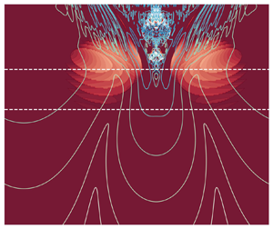
3.4. Eigenfunctions
Further insights into these SIC instabilities are gained by examining their eigenfunctions expressed in (2.7) for representative cases (see figure 2 and table 1). Note that the shape of the eigenfunction might change slightly depending on the selected linear mode. In figure 5, we present the vorticity (figure 5a,c,e,g,i) and density (figure 5b,d,f,h,j) eigenfunctions of the fastest growing modes for cases I,…, V, marked in figure 2, each of which represents one of the five branches of instabilities: HWI, KHI, LWI, DVLWI and UVLWI, respectively. Note that the  $x$ axis in these cases has been rescaled to compare modes having very different wavelengths. In figure 5, the wavelengths of HWI and KHI are, approximately, $4$, while LWI, DVLWI, and UVLWI are $70$,
$70$,  $300$ and $420$, respectively.

The density eigenfunctions of all modes are concentrated near the interface, indicating the critical role of stratification. Near the walls, the intensity of vorticity eigenfunctions is large due to the no-slip effects of the walls. (Note that, with a free-slip velocity boundary condition, the corresponding modes do not exhibit this intense vorticity at the wall, see the Appendix A.) In the shear layer, one of the HWI modes plotted here (left-propagating) exhibits two pairs of counter-rotating roll cells centred at  $z\approx 0.5$. For KHI, the vorticity and density eigenfunctions are highly concentrated at the interface, leaving a weaker bulk region in the rest of channel. By contrast, the vorticity eigenfunctions of LWI, DVLWI and UVLWI fill the channel.
3.5. Neutral boundaries of instabilities
As mentioned in § 3.1, different families of instabilities can coexist at the same parameters, making it difficult to determine the neutral boundary of each family from the distribution of fastest growing modes in figure 2. To identify the different neutral boundaries we employ the unsupervised machine learning algorithm DBSCAN (density-based spatial clustering of applications with noise) (Ester et al. Reference Ester, Kriegel, Sander and Xu1996). The DBSCAN algorithm clusters the local maxima of the dispersion relation (figure 3a) of all the cases in figure 2 using  $k$,
$k$,  $\eta _r$ and $\eta _i$ as input variables. These variables are first logarithmically transformed and normalised before being fed into DBSCAN for clustering. Note that DBSCAN groups the local optimal modes of LWI and UVLWI together in a single cluster due to their similarity in $k$,
$k$,  $\eta _r$ and $\eta _i$. An additional step is taken to distinguish between the two branches by using the fact that LWI occurs when $\theta >0$, while UVLWI occurs when $\theta <0$.
The clustering analysis in figure 6(b–f) reveals the regimes of different families of instabilities, which could not have been identified by simply looking at the distribution of fastest amplifying modes (figure 6a). The KHI regime (figure 6c) exactly matches the distribution of the fastest amplifying modes (figure 6a), while other modes (LWI, DVLWI, UVLWI) that overlap with KHI are omitted. This suggests that KHI always has the fastest growth rate. For HWI (figure 6b), increasing  $\theta$ clearly decreases the growth rate while shrinking its ‘territory’, causing it to disappear when $\theta >2^\circ$. When $\theta$ is fixed, the fastest growing HWI appears at $Ri_b\approx 1$, while the growth rate decreases as $Ri_b$ departs from $1$. The territory of HWI overlaps with UVLWI (figure 6f) which can exist when $\theta <-0.5^\circ$. The growth rate of these two modes is comparable so that figure 6(a) cannot display the neutral boundaries of these two modes properly. As for LWI (figure 6d), it generally persists at large positive $\theta$ except for $Ri_b\lesssim 0.2$. The critical $\theta$ for the appearance of DVLWI (figure 6e) is $\approx 2.5^\circ$. It overlaps with KHI and LWI at large $\theta$ and small $Ri_b$, respectively, but is mostly omitted in the plot of the fastest growing mode due to its relatively small growth rate.

Figure 6. Clustering results – fastest growing mode of each family in  $Ri_b-\theta$ parameter space: (a) fastest amplifying modes (FAM) of all families reproduced from figure 2(a); (b) HWI; (c) KHI; (d) LWI; (e) DVLWI; and (f) UVLWI modes.
In general, these long-wave families of instabilities can persist across a wide range of  $Ri_b$, ranging from $Ri_b\ll 0.25$ (especially for DVLWI and UVLWI) to $Ri_b\gg 1$. Consequently, we anticipate their widespread presence in sloping stratified exchange flows.
3.6. Effect of Reynolds and Prandtl numbers
In this section, we study the impacts of Re and Pr on these different families of instabilities.
3.6.1. Reynolds number effects
Figure 7 shows the  $Ri_b-\theta$ parameter space of the fastest growing modes at a lower ${\textit {Re}}=650$ (figure 7a) and higher ${\textit {Re}}=5000$ (figure 7b) than the standard case discussed in § 3.1. Generally, ${\textit {Re}}$ has a significant effect on all families of instabilities except KHI. The HWI-dominated regime expands to smaller (and slightly larger) $Ri_b$ but shrinks in $\theta$ with increasing ${\textit {Re}}$. The largest $\theta$ for HWI decreases from $1.3$ to $0.4$, indicating a stronger suppression effect by the slope. The long-wave families (LWI, DVLWI and UVLWI) still dominate the large $Ri_b$ region, and their boundaries approach $\theta =0^\circ$ as ${\textit {Re}}$ increases. For instance, the left-most VLWI appears at $\theta \approx 2^\circ$ for ${\textit {Re}}=650$, whereas it is $\theta \approx 0.3^\circ$ for ${\textit {Re}}=5000$. Similarly, for UVLWI, the right-most points change from $\theta=-0.6^\circ$ at ${\textit {Re}}=650$ to $\theta =-0.1^\circ$ at ${\textit {Re}}=5000$. It is anticipated that in the inviscid limit ${\textit {Re}}\rightarrow \infty$ the critical $\theta$ will approach $0$. Therefore, it is a reasonable speculation that these gravity-induced long waves may be generic in high- ${\textit {Re}}$ natural water bodies subjected to shear, stratification and even the shallowest slope.

Figure 7. Effect of the Reynolds number: fastest growing mode projected onto  ${Ri_b}-\theta$ space for (a) ${\textit {Re}}=650$ and (b) ${\textit {Re}}=5000$.
3.6.2. Prandtl number effects
Figure 8 displays the  $Ri_b-\theta$ parameter space of the fastest growing modes at ${\textit {Pr}}=1$, $28$ and $70$, respectively, corresponding to the increasingly sharper interface of the density base state, following (2.10). To ensure convergence, the grid resolution for the LSA was set to $150$, $250$ and $400$, respectively. As ${\textit {Pr}}$ increases, the influence of the slope $\theta$ on KHI becomes more significant, resulting in a wider upper boundary of KHI, which can be triggered at $Ri_b>0.25$ for large downward slopes $\theta \gtrsim 5^\circ$. Meanwhile, HWI is also significantly affected by ${\textit {Pr}}$. At ${\textit {Pr}}=1$, HWI does not appear due to the thick density interface determined by (2.10). However, as ${\textit {Pr}}$ increases, the region of HWI expands significantly towards larger $\theta$. The long-wave families exist at all ${\textit {Pr}}$. As ${\textit {Pr}}$ increases from ${\textit {Pr}}=1$ to $28$, the territory of the long waves converges towards $\theta =0$. However, the changes in the territory become less significant from ${\textit {Pr}}=28$ to $70$, indicating a potential convergence of the wave regime at moderate ${\textit {Pr}}$. However, due to the dominance of HWI at high ${\textit {Pr}}$, the long-wave families are largely omitted by the fastest growing HWI at $Ri_b\lesssim 10$ in figure 8(c). Note that the impact of Pr may be attributed to two factors: (a) the modification of interface thickness and (b) the change in $\mathcal {L}_{\rho \rho }$ of (2.9). Although not presented here, we observed that those short-wave instabilities are more sensitive to changes in the interface thickness, while long-wave instabilities are influenced by both factors. In practical flow systems, such as the SID studied by Lefauve & Linden (Reference Lefauve and Linden2020), ${\textit {Pr}}$ and the interface thickness are often coupled, as a large ${\textit {Pr}}$ reduces the scalar diffusivity, enabling the maintenance of a relatively sharp interface. Finally, at ${\textit {Pr}}=28$, the profile of the Thorpe exchange flow ( $\mathcal {F}=0$ in 2.12) passes sequentially through the HWI-, DVLWI-, LWI- and KHI-dominated regimes. This provides an example where DVLWI and LWI can dominate Thorpe's SIC flow.

Figure 8. Effect of Prandtl number: fastest growing mode projected onto the  ${Ri}_b-\theta$ space for (a) ${\textit {Pr}}=1$, (b) ${\textit {Pr}}=28$ and (c) ${\textit {Pr}}=70$, respectively.
4. Nonlinear evolution of unstable modes
To gain insight into the subsequent nonlinear evolution of these unstable modes we conduct forced 2-D DNS. We describe our DNS in § 4.1 and discuss the evolution and breakdown of the instabilities in § 4.2. The instantaneous flow kinetics and the mechanisms leading to breakdown are discussed in §§ 4.3 and 4.4, respectively.
4.1. Forced DNS formulation
To simulate the growth of linear unstable perturbations on the desired base state, we add to the right-hand sides of (2.2) and (2.3) the two forcing terms
 \begin{equation} F_v ={-}\frac{1}{{\textit{Re}}}\frac{{\rm d}^2 U}{{\rm d} z^2}-Ri\sin\theta R, \quad F_\rho ={-}\frac{1}{{\textit{Re}}{\textit{Pr}}}\frac{{\rm d}^2 R}{{\rm d} z^2}, \end{equation}
respectively, derived from the steady non-convective base flow equations. In this way, the mean velocity and density of the DNS are forced towards the targeted base profile of  $U(z)$ and $R(z)$, while the effects on the evolution of perturbations are eliminated. These terms can be regarded as enforcing a pressure-driven exchange flow under a sustained stratification. Similar approaches that apply constant body forces to the stratified flows were introduced in Howland, Taylor & Caulfield (Reference Howland, Taylor and Caulfield2018) and Parker, Caulfield & Kerswell (Reference Parker, Caulfield and Kerswell2021).
We perform the simulations using Dedalus (Burns et al. Reference Burns, Vasil, Oishi, Lecoanet and Brown2020), an open-source solver widely used to solve various fluid problems (Lecoanet et al. Reference Lecoanet, McCourt, Quataert, Burns, Vasil, Oishi, Brown, Stone and O'Leary2016; Beneitez, Page & Kerswell Reference Beneitez, Page and Kerswell2023; Zhu, Li & Marston Reference Zhu, Li and Marston2023c). Dedalus employs a Fourier–Chebyshev pseudospectral scheme for spatial discretisation and a third-order, four-stage diagonally implicit–explicit Runge–Kutta scheme (Ascher, Ruuth & Spiteri Reference Ascher, Ruuth and Spiteri1997) for time stepping. We imposed periodic boundary conditions in the streamwise  $x$ direction, while we applied no-slip and no-flux boundary conditions for velocity and density, respectively, to the solid walls at $z=\pm 1$, as in the LSA. The streamwise length $L_x$ of the channel was set equal to the wavelength of the fastest growing mode, while the channel height $L_z$ was fixed at $2$. We employed a uniform grid for the $x$ direction and a Chebyshev grid for the $z$ direction. The simulation resolution was determined by the geometrical and physical parameters of the problem. We initialised the simulations by superimposing on the base state the eigenfunctions of the LSA unstable modes with a perturbation magnitude $\zeta$. Note that the evolution of these DNS does not depend on the specific eigenfunction perturbations. For instance, a sufficient small random initial perturbation can evolve into the dominant unstable modes after a longer initial evolution. The parameters of the production runs are listed in table 1.
4.2. Temporal evolution
In this section, we focus on the temporal evolution of the fastest growing modes of each instability family, I, II, III, IV and V, as marked in figure 2. Figure 9 shows the temporal behaviour of the unstable modes through the time series of the mass flux  $Q_m(t)$ (3.2) and the spatially averaged vertical velocity of perturbations $\langle w^2 \rangle (t)$, where $\langle \boldsymbol {\cdot } \rangle$ denotes averaging over $x,z$. The magnitude $\zeta$ of the perturbation was chosen differently for each mode in order to obtain a reasonably long linear growth period. The forcing magnitude $\gamma$ is determined so that the base velocity matches the selected cases in figure 2. The exchange flow is simulated by forcing the background flow in time using (4.1a,b) and allowing the perturbations to grow.

Figure 9. Time evolution of (a) mass flux  $Q_m$ and (b) logarithm of vertical velocity squared $\ln \langle w^2\rangle$ for the fastest growing modes in table 1. The slopes of the growth for the HWI, KHI, LWI, DVLWI and UVLWI modes are $0.0038$, $0.15$, $0.018$, $0.0017$ and $0.0089$, respectively, consistent with $2\eta _r$ of corresponding unstable mode in LSA ( $0.0037$, $0.15$, $0.018$, $0.00018$ and $0.0092$).
In figure 9(a),  $Q_m$ is initially constant, consistent with the targeted base state in figure 2. This suggests that the body forces described in (4.1a,b) effectively control the background state. However, the $Q_m$ profiles cease to remain flat when the perturbations experience significant amplification, marking the onset of the nonlinear stage in the flow. The evolution of the disturbance amplitudes is shown in figure 9(b), with all cases exhibiting a clear exponential growth period for $w^2$, with growth rates matching the corresponding linear unstable modes. It suggests a minor impact of the forcing, introduced by (4.1a,b), on the evolution of these unstable modes. For KHI, LWI and UVLWI, following the exponential growth period, an intense nonlinear bursting process is caused by the breakdown of the primary waves, leading to intense mixing and changes in $Q_m$ and $w^2$. In contrast, the sudden changes in $Q_m$ do not appear for HWI and DVLWI since their primary waves do not break down. The HWI and DVLWI have a pair of conjugate modes, represented by oscillating $w^2$ profiles, due to the synchronisation of complex-conjugate modes, as discussed in Yang et al. (Reference Yang, Tedford, Olsthoorn, Lefauve and Lawrence2022). Interestingly, after the nonlinear bursting at $t=1250$, the nonlinear HWI still maintains the oscillating pattern (Lefauve et al. Reference Lefauve, Partridge, Zhou, Dalziel, Caulfield and Linden2018). The time series of $Q_m$ and $\ln \langle w^2\rangle$ pinpoint the critical time when the nonlinear effects become prominent. Specifically, this occurs when $Q_m$ deviates from its constant level or when $\ln \langle w^2\rangle$ no longer shows exponential growth after reaching a certain amplitude. Note that the critical amplitude for nonlinear bursting remains independent of the initial amplitude of perturbations. However, it varies for each individual unstable mode, as illustrated in figure 9. The critical time may vary depending on the particular unstable mode, the growth rate and the magnitude of the initial perturbation.
Figure 10 shows the  $x-t$ diagrams of $\ln \langle w^2\rangle _{z}$, where $\langle \cdot \rangle _{z}$ indicates $z$-averages. In case HWI (figure 10a), we observe left-going waves from the spatial–temporal diagram, while its conjugate pair is omitted as only one mode of the pair is imposed as initial perturbation in the DNS. Nonlinear effects become significant at $t\approx 1250$ ( $\ln {\langle w^2 \rangle }\approx -9$) owing to a relatively small growth rate ( $0.0038$), as indicated by the saturation of the exponential growth of $w^2$ in figure 9(b). Interestingly, the spatial–temporal pattern of HWI does not change significantly after $t\approx 1250$ in figure 10(a). This implies that nonlinear effects only halt the linear growth of Holmboe wave structures, which maintain their forms as nonlinear Holmboe waves, as observed in experiments and nature (Tedford, Pieters & Lawrence Reference Tedford, Pieters and Lawrence2009; Meyer & Linden Reference Meyer and Linden2014; Cudby & Lefauve Reference Cudby and Lefauve2021). By contrast, KHI generates strong secondary instabilities (Mashayek & Peltier Reference Mashayek and Peltier2012) after the onset of nonlinear effects at $t\approx 200$ ( $\ln {\langle w^2 \rangle }\approx -5$). Consequently, the KH billows break up, leading to highly chaotic flow stages with small-scale structures.

Figure 10. Spatial–temporal diagrams of  $\ln \langle w^2\rangle _{z}$ from the nonlinear simulations of (a) HWI, (b) KHI, (c) LWI, (d) DVLWI and (e) UVLWI. The black solid lines indicate the times of visibly nonlinear dynamics identified in figure 9.
In figure 10(c–e), the  $x-t$ diagrams of $\ln \langle w^2\rangle _{z}$ reveal that for the three new families of long waves, small-scale structures emerge in the latter stages of the transitions, characterised by highly fluctuating contour lines. In the case of LWI (figure 10c), the onset of an intense chaotic flow period occurs at $t=710$, during which small-scale structures are initially generated at $x=25$ and $x=55$ where $\ln \langle w^2\rangle _{z}$ of the linear wave peaks. These structures then propagate towards the quiet regions and ultimately trigger a disorganised flow field across the channel. Interestingly, we have observed from figure 9(a) that the nonlinear effects set in at $t=630$ ( $\ln {\langle w^2 \rangle }\approx -14$) as $Q_m$ significantly deviates from the original constant level. At this stage, the two peaks of the linear disturbance approach each other while contour curves twist. The $\ln \langle w^2\rangle _{z}$ distribution no longer maintains its shape as is in the linear growing period. As we will show later, this nonlinear dynamics is the breakdown of the long waves.
In case DVLWI, as shown in figure 10(d), the unstable wave moves leftward and grows exponentially until nonlinear dynamics set in at  $t=2860$ ( $\ln {\langle w^2 \rangle }\approx -19$), which is identified by a jump in $\langle w^2 \rangle (t)$ in figure 9(b). Small-scale waves/structures are formed at a local peak of the long wave $w^2$, which propagate both leftward and rightward, creating strong mixing. Despite the intense bursting of the flows, the long wave does not break down like LWI, presumably due to its low growth rate. It continues to propagate at the same phase speed as the linear wave energy that was previously used to amplify the long wave and is then fed to the small-scale waves, which eventually break down and dissipate, allowing the long wave to persist for a long period of time and propagate over a long distance.
In case UVLWI (shown in figure 10e), local nonlinear bursting and small-scale structures are directly created at  $t=500$ ( $\ln {\langle w^2 \rangle }\approx -16$) and $x\approx 150$ and $350$ on top of the long wave. Similar to DVLWI, a preliminary breakdown of the long-wave is not observed. Soon after, intense secondary instabilities fill the entire channel and the long waves are no longer distinguishable.
The evolution of long waves and the consequent generation of short waves are illustrated in figure 11, depicting the evolution of the spectrum of TKE:
 \begin{equation} E_k(k,t)=\tfrac{1}{4}\int_{{-}1}^{1} ({\tilde u}^{\prime \circledast}{\tilde u}^{\prime} + {\tilde w}^{\prime \circledast}{\tilde w}^{\prime} ) \,{\rm d}z, \end{equation}
where superscript  $\circledast$ denotes the complex conjugate and tildes indicate a Fourier transform of the perturbation velocity fields $u',w'$ with respect to $x$. In all cases, prominent red contours initially emerge at the smallest wavenumber $k$, highlighting the prevalence of long waves with peaks at $k\approx 10^{-1}$, $10^{-2}$ and $10^{-2}$ for LWI, DVLWI and UVLWI, respectively. The energy spectrum then gradually extends towards larger wavenumbers $k$ before the onset of the nonlinear bursting process (dashed line), during which small-scale structure rapidly expands at large $k$. The LWI spectrum expansion is smoother than the others, corresponding to its two-stage transition. Meanwhile, small-scale structures appear at $(k,t)=(2,500)$ in UVLWI before the entire spectrum is filled, representing a sequence of regular KH-like billows.

Figure 11. Evolution of the turbulent kinetic energy (TKE) spectrum  $E_k$ in wavenumber–time space for nonlinear DNS in three long wave cases: (a) LWI; (b) DVLWI; (c) UVLWI. The black dash lines mark the times of visibly nonlinear dynamics identified in figure 9.
Essentially, the nonlinear growth of long waves alters the base state and allows the growth of short-wave instabilities. We will explore this mechanism in more detail in §§ 4.3–4.4.
4.3. Features of flow kinematics
In this section we present instantaneous flow fields corresponding to the key stages of evolution of the long wave instabilities. The kinematics of the short waves, i.e. HWI and KHI, have been well-documented in the literature (Smyth & Winters Reference Smyth and Winters2003; Mashayek & Peltier Reference Mashayek and Peltier2012, Reference Mashayek and Peltier2013; Salehipour et al. Reference Salehipour, Peltier and Mashayek2015; Lefauve et al. Reference Lefauve, Partridge, Zhou, Dalziel, Caulfield and Linden2018), and will not be repeated here.
Figure 12 shows snapshots of the total density  $\rho =R+\rho ^\prime$ (colours) and vertical velocity $w^\prime$ (lines) at four stages of LWI. We find two stages of nonlinear breakdown corresponding to the breakdown of the long wave and the generation of KH-like overturns. At the linear stage (figure 12a), the impacts of the density perturbation on the mean are barely observable and the interface is thin and flat. Later, the growth of LWI raises and drops on the left- and right-hand sides of $x=40$, creating a large-scale jump (figure 12b). Interestingly, a hydraulic jump is also observed in the experiments and DNS of SID (Zhu et al. Reference Zhu, Atoufi, Lefauve, Taylor, Kerswell, Dalziel, Lawrence and Linden2023a,Reference Zhu, Jiang, Lefauve, Kerswell and Lindenb) and may be related to LWI given the analogous length scale between the SID facility ( ${\sim }60$) and the unstable waves. Meanwhile, $w^\prime$ becomes localised at $x=40$. Further amplification of the unstable mode breaks down the jump, generating a chaotic region at $t=700$. At this stage, the instability is no longer linear, as demonstrated in § 4.2. At $t=760$, a series of short overturns resembling KH billows are formed inside and at two sides of the chaotic region at $x=40$. These waves propagate away from the chaotic region and may eventually lead to (2-D) turbulence.

Figure 12. Nonlinear LWI – density (colour) and vertical velocity (lines) snapshots of the forced DNS at different time instances: (a)  $t=400$; (b) $t=600$; (c) $t=700$; (d) $t=760$.
Figure 13 shows snapshots of the flow fields at three stages of DVLWI. From  $t=1500$ (figure 13a) to $t=2500$ (figure 13b), DVLWI amplifies, while light-blue (e.g. upper layer, $150< x<200$) and light-red (e.g. bottom layer, $250< x<300$) regions become distinguishable, indicating the enhancement of mixing in these regions which acts to dissipate the energy injected by gravity. As the base flow is frozen by the simulation, the mixing is attributed to the amplification of DVLWI. At $t=2900$ (figure 13c), further growth of the long wave induces intense KH-like overturns near the leading edge of DVLWI, characterised by the strong fluctuation of $w^\prime$ in the range of $x=175\sim 250$. These overturns create extra dissipation and mixing of the flow, acting to balance the extra kinetic energy supplied by gravity. In contrast to the KH-like overturns in LWI, the overturns can centre within the bulk flow of each layer in addition to the interface (figure 13d). This is because the propagation of the leading edge of the long waves (dark blue region at $x=180$) into the mixed region (light blue region at $x<180$) creates a weak interface between the denser and lighter regions inside the flow layer.

Figure 13. Nonlinear DVLWI – density (colour) and vertical velocity (lines) snapshots of the forced DNS: (a)  $t=1500$; (b) $t=2500$; (c) $t=2900$. An enlarged plot of panel (c) is shown in panel (d).
Finally, in the UVLWI case (figure 14), the amplification of the stationary waves directly induces localised KH-like billows characterised by strong fluctuations of  $w^\prime$ in figure 13(c) at the interface without first breaking down as in LWI. This behaviour may be due to the faster growth rate, which prevents the formation of a distinct nonlinear ‘jump’ observed in LWI.

Figure 14. Nonlinear UVLWI – density (colour) and vertical velocity (lines) snapshots of the forced DNS: (a)  $t=600$; (b) $t=888$. An enlarged plot of panel (b) is shown in panel (c).
As discussed in § 4.2, the evolution of these long wave families eventually lead to intense bursting processes that form strong small-scale KH-like overturns. These overturns are responsible for dissipating the kinetic energy injected by a positive slope or a background forcing that cannot be completely balanced by the dissipation of long waves. Note that in all the long waves cases, a short-wave instability (KHI and HWI) does not initially exist according to the LSA in § 3.1. In the next section, we study how these short-wave KH-like overturns are induced by nonlinear long waves.
4.4. Breakdown mechanism
In § 3.1, we showed that the KHI can only occur when  $Ri_b\lessapprox 0.25$. In the new long wave cases considered in this study, $Ri_b\gg 1$, hence KHI cannot be triggered. Instead, KH-like overturns are formed by the nonlinear evolution of these long waves.
To understand the cause of the formation of KH-like overturns, we computed the gradient Richardson number  $Ri_g$ at the total density interface $\rho =0$, which is defined as
 \begin{equation} \left. Ri_g(x,t) \equiv {\textit{Ri}} \frac{\partial \rho/\partial z}{(\partial u/\partial z)^2}\right|_{\rho=0}, \end{equation}
where we recall that  $Ri\equiv 1/4$ (see § 2.1). Note that the field $Ri_g(x,t)$ is based on the total velocity $u$ and density $\rho$, and thus differs from the constant $Ri_b$ defined in (3.1), which is based on the initial base flow profiles $U$ and $R$.
$R$.
In figure 15, we show the  $x-t$ diagrams of $Ri_g$, with $w^2$ contour lines superimposed. In general, as the unstable long waves grow, the density gradient can decrease due to diffusivity which increases the mixing layer. Meanwhile, the velocity gradient can increase as the perturbations are amplified. This results in a decreasing interfacial $Ri_g$, until it reaches below $0.25$ (shades of blue), with which small-scale structures are associated.

Figure 15. Spatial–temporal diagrams of the gradient Richardson number  $Ri_g$ at the density interface in forced DNS for (a) LWI, (b) DVLWI and (c) UVLWI. The colour maps show the values of $Ri_g$, while the lines represent $ln\langle w^2\rangle _{z}$.
For each individual long-wave family, the process is slightly different. The LWI (figure 15a) has two stages of nonlinear breakdown. The first stage appears at  $t=680$ when a ‘jump’ is formed at $x=45$. This jump changes the density interface and generates two low $Ri_g$ regions separated by a high $Ri_g$ region. In these low $Ri_g$ regions, $Ri_g$ continuously decreases due to the amplification of long waves and eventually reduces below $0.25$, which potentially allows the growth of the secondary KHI in these regions. Finally, overturns are formed in these regions, leading to the second stage of nonlinear breakdown. Similarly, the amplification of DVLWI (figure 15b) also causes a low $Ri_g$ region that travels along with the waves. As soon as $Ri_g<0.25$, intense overturns are formed in this region and later contaminate the entire duct. For UVLWI, the overturns are first formed at the edges of the low $Ri_g$ region ( $170< x<330$). The close relation between the low $Ri_g$ region and the onset of nonlinear short waves strongly suggests that the overturns are a consequence of the decreasing of local $Ri_g$ caused by the nonlinear evolution of initially long waves.
From an energy budget perspective, the formation of short-wave overturns in these long-wave simulations allows for more efficient dissipation of kinetic energy fed by external forces. In figure 16(a), we illustrate the pathways of TKE  $K^\prime$ as given schematically by
 \begin{equation} \partial_t K^\prime=\varPhi^{K^\prime}+P-B-\epsilon, \end{equation}
where,  $P$,
$P$,  $\epsilon$, $B$ and $\varPhi ^{K^\prime }$ represent the production, dissipation, buoyancy flux, and transport terms of $K^\prime$. The reader may refer to Caulfield (Reference Caulfield2021) and Lefauve & Linden (Reference Lefauve and Linden2022) for the definition and a more comprehensive discussion of the kinetic budget of stratified shear flows. Under strong stratification $Ri_b\gg 0.25$; initially only the long waves are allowed to grow, gaining energy from the mean flow through P and B, and losing it through $\epsilon$. As the long waves are amplified, local shear is created and amplified by the growing velocity perturbations, leading to a local decrease of $Ri_g$. As $Ri_g\lesssim 0.25$, the necessary condition for the growth of short waves (mostly KHI here) becomes satisfied. The short waves then grow, extracting $K^\prime$ from the long waves and dissipating it to internal energy. This opens a new energy pathway that allows flows with strong stratification (large $Ri_b$) to dissipate energy by creating small-scale (turbulent) structures. When $Ri_b\ll 0.25$ (figure 16b), long waves can coexist with short waves (e.g. case IV in figure 3) and may contribute to the energy dissipation. But they are often significantly weaker than short waves, which tend to have a faster growth rate. Meanwhile, the short wave directly gains most of the kinetic energy from the mean flow and converts it to internal energy. We also note that turbulence created by these unstable waves can also induce irreversible mixing which, in return, contributes to the production of internal energy.

Figure 16. Pathways of TKE in sloping exchange flows under (a) strong stratification  $Ri_b \gg 0.25$, where only very long waves are unstable; (b) weaker stratification $Ri_b< 0.25$ where both short and long waves coexist.
5. Conclusions
In this paper, we examined the effects of longitudinal gravitational forces on the stability of two-layer stratified exchange flows by conducting linear stability analyses and nonlinear forced DNS in a sloping channel with solid top and bottom boundaries. In addition to the well-known HWI and KWI, we revealed the existence of three new families of long-wave instabilities subject to non-zero gravitational forces ( $\theta \neq 0$):
(i) LWI, with wavelengths of the order $10- 100$ channel depths and a near-zero wave speed (see figure 12);
(ii) DVLWI, with wavelengths of the order
$100- 1000$ channel depths, a non-zero wave speed, and complex conjugate eigenmodes implying travelling waves (see figure 13);(iii) UVLWI, with wavelengths
$\geqq 100$ channel depths and a near-zero wave speed (see figure 14).


These long-wave families are generically different from the HWI and KHI instabilities. They are primarily initiated by interactions between the streamwise gravity forcing and gravity waves, with shear playing a secondary role. Therefore, their onset is largely independent of the base flow speed, meaning that they can be triggered even at very high background gradient Richardson numbers  $Ri_b\gg 1$, and induce chaos, (2-D) turbulence and mixing even in strongly stratified fluids. In a weakly stratified flow (low $Ri_b$), they can also coexist with short-wave instabilities (KHI and HWI), but they generally have a lower growth rate. Meanwhile, increasing the slope $\theta$ tends to suppress the HWI regime while enhancing the KHI. The neutral boundary of KHI increases linearly from $Ri_b=0.15$ at $\theta =-10^\circ$ to $0.25$ at $\theta =10^\circ$.
To explore the dependence of the long-wave families on flow parameters, we varied the Reynolds number  ${\textit {Re}}$, Prandtl number ${\textit {Pr}}$, the base flow and boundary conditions. While increasing the ${\textit {Re}}$ does not significantly affect KHI, it does enhance the other instabilities. The range of HWI expands to larger $Ri_b$, while the range of the long-wave instabilities approaches $\theta =0$. Therefore, it can be anticipated that as ${\textit {Re}}\rightarrow \infty$ (as is often the case in natural flows), the critical slope required to trigger these long instabilities approaches zero. By increasing ${\textit {Pr}}$, the range of the long-wave instabilities slowly approaches $\theta =0$, indicating that these long waves can exist in both water ( ${\textit {Pr}}\approx 7\sim 700$) and air ( ${\textit {Pr}}\approx 1$). It should be noted that these instabilities are not limited to the sine-like base state and the no-slip boundary conditions used in this study. Instead, they can be triggered by, for example, a $\tanh$-shaped velocity base and free-slip velocity boundary conditions.
Finally, we studied the nonlinear evolution of the different instabilities and their connections to turbulence using a 2-D forced DNS. For all of the long-wave instabilities, the evolution eventually led to a nonlinear bursting process with significant small-scale secondary KH-like overturns and mixing. Specifically, the LWI exhibits two nonlinear stages where an initial breakdown of the long waves is followed by a secondary bursting process, creating intense KH-like overturns. For DVLWI and UVLWI, the long waves do not break down. Instead, they directly alter the base states and induce localised small-scale overturns.
The evolution of these long instabilities results in a decrease in the density gradient and an increase in the shear, which in turn reduces the local gradient Richardson number  $Ri_g$. Our analysis reveals that the appearance of KH-like overturns is highly correlated with a local low $Ri_g$, which approaches the critical threshold of $0.25$ (below which we find the KHI), substantiating the emergence of localised KH-like overturns. From a TKE budget perspective, a new energy pathway allows the transfer of kinetic energy from the mean flow to the long waves (linearly) and then to the short waves (nonlinearly), eventually leading to the dissipation of TKE, under conditions where short waves would be initially linearly stable.
The circumstances under which turbulence can persist in strongly stratified flows remains a fascinating debate within the community (Caulfield Reference Caulfield2021). We demonstrated that weakly unstable (very) long waves may trigger turbulence and mixing after long periods of time, even under initially very strongly stratified conditions ( $Ri_b\gg 1$). Reproducing these phenomena in experiments might pose a challenge due to their exceptionally long length and temporal scales, except for LWI, which might exhibit a comparable length with the existing SID experiments. However, they have particular relevance for high- ${\textit {Re}}$ flows in rivers (Yoshida et al. Reference Yoshida, Ohtani, Nishida and Linden1998) and straits (Gregg & Özsoy Reference Gregg and Özsoy2002) or any natural flow having even very shallow slopes $\theta \approx 0$. A quantitative investigation of the turbulent transition and mixing associated with these long waves would require 3-D stability and DNS, an endeavour left for future work.
Funding
We acknowledge the ERC Research and Innovation grant no. 742480, ‘Stratified Turbulence And Mixing Processes’ (STAMP). A.L. acknowledges a Leverhulme Trust Early Career Fellowship and a NERC Independent Research Fellowship (NE/W008971/1).
Declaration of interests
The authors report no conflict of interest.
Appendix A. Linear stability analysis with free-slip boundary condition
To investigate the potential impacts of the base flow shape on the instabilities, we perform a LSA with a  $\tanh$-shaped density (2.10) and velocity base
 \begin{equation} U(z)=\gamma\tanh(\iota z), \end{equation}
where  $\iota =1.5\kappa \sqrt {Pr}$ defines the thickness of velocity base. A free-slip boundary condition for velocities is also adopted to understand the effects of boundary conditions.
In figure 17, we show the  $Ri_b-\theta$ and $Q_m-\theta$ parameter space of the fastest growing modes of the above LSA. Clearly, the five families of instabilities appear even with the different base flow and boundary conditions. This means that these instabilities are not a consequence of an arbitrary flow condition that is subject to a certain base flow or boundary condition, but rather general flow instabilities that can appear in a wide range of stratified flow systems. Features of these instabilities, e.g. the wave speed, wavelength, growth rate and regime, are largely consistent with the main cases discussed in § 3.1 (see figure 2a,c), which suggests, again, the universal features of these instabilities.

Figure 17. Impact of a tanh-shaped density and velocity profiles; projection of the fastest growing mode onto parameter spaces: (a)  ${Ri}_c-\theta$ and (b) $Q_m-\theta$. Solid and dashed lines are the growth rate and frequency, respectively (compare with figure 2a,c).
Figure 18 shows the eigenfunctions of fastest growth modes of the typical case of each instability (marked in figure 17). Note again that the forms of eigenfunctions of each instability are generally consistent with the main cases in § 3.4 in the middle region of the channel (see figure 5). However, those intense regions near the wall do not appear with a free-slip velocity boundary condition. Therefore, these near-wall structures as well as the no-slip boundary conditions are not essential to these instabilities.

Figure 18. Impact of a tanh-shaped density and velocity profiles: vorticity (a,c,e,g,i) and density (b,d,f,h,j) eigenfunctions of the fastest growing modes of (a,b) I, HWI, (c,d) II, KHI, (e,f) III, LWI, (g,h) IV, DVLWI and (i,j) V, UVLWI (compare with figure 5).


 Open access