


1. Introduction
Interest in gravity-driven flows of viscous fluids spans the fields of geophysics, geology and industrial engineering, involving a range of environmental and industrial phenomena (Simpson Reference Simpson1967, Reference Simpson1982; Benjamin Reference Benjamin1968; Hoult Reference Hoult1972; Linden Reference Linden1999; Huppert Reference Huppert2006). Such flows feature striking dynamics when they involve the superposition of one viscous fluid over another, particularly when the underlying fluid is less viscous (Kowal & Worster Reference Kowal and Worster2015; Kumar et al. Reference Kumar, Zuri, Kogan, Gottlieb and Sayag2021). These are relevant to the flow of large-scale, glacial ice sheets over till, or a mixture of clay and subglacial sediments (Weertman Reference Weertman1957, Reference Weertman1964; Nye Reference Nye1969; Kamb Reference Kamb1970; Fowler Reference Fowler1981; Engelhardt et al. Reference Engelhardt, Humphrey, Kamb and Fahnestock1990; Kyrke-Smith, Katz & Fowler Reference Kyrke-Smith, Katz and Fowler2014), the flow of layers of lava (Balmforth & Craster Reference Balmforth and Craster2000) and layered flows in porous media (Woods & Mason Reference Woods and Mason2000), for example.
The glacial analogue involves the flow of a power-law fluid representing ice, the rheology of which is commonly referred to as Glen's flow law in the glaciological literature (Glen Reference Glen1955). It is more difficult to quantify the rheology of subglacial till, though frequently adopted rheologies for till include a plastic rheology with a Mohr–Coulomb yield stress, relevant on the small scales (Kamb Reference Kamb1970; Tulaczyk, Kamb & Engelhardt Reference Tulaczyk, Kamb and Engelhardt2000; Kamb Reference Kamb2001), or a viscous power-law rheology, relevant to large scales of kilometres or more (Boulton & Hindmarsh Reference Boulton and Hindmarsh1987; Hindmarsh Reference Hindmarsh1997). However, recent work by Tulaczyk (Reference Tulaczyk2006) suggests that the difference between the rheology at small and large scales is not at all clear, as observations of the subglacial till beneath the well-lubricated Whillans Ice Stream, West Antarctica, indicate that its rheology is independent of scale. These observations have been made possible following short speed-up events on the ice plain of Whillans Ice Stream, which provided the opportunity to examine the in situ rheology of till beneath Whillans Ice Stream, integrated over roughly 10–100 km, and compare it to the rheology of small laboratory samples of till from beneath the same ice stream.
We investigate the gravity-driven flow of two superposed thin films of viscous fluids of power-law rheology in two-dimensional and axisymmetric geometries. The flow reduces to that of Kowal & Worster (Reference Kowal and Worster2015) in the Newtonian limit. We model the flow using lubrication theory by balancing viscous and buoyancy forces, and we assume that inertial effects and the effects of mixing and surface tension at the interface between the layers are negligible. Although it is possible to generalize our work to a mathematical model for which the rheology of the two viscous fluids involves power-law exponents that may, in general, be unequal, we focus on the case in which the two power-law exponents are equal. The flow is self-similar in this scenario in both geometries.
Four distinct flow regimes emerge, from thin films of viscous fluid lubricating a more viscous fluid from below, akin to flows over slippery substrates such as the flow of glacial ice over till, to thin films of fluid coating a more viscous fluid from above, and thin films of fluid forming a more viscous crust over the main current, akin to viscous-gravity currents with a solidifying crust (Fink & Griffiths Reference Fink and Griffiths1990; Griffiths & Fink Reference Griffiths and Fink1993; Fink & Griffiths Reference Fink and Griffiths1998; Balmforth & Craster Reference Balmforth and Craster2000). In contrast to thin films coating a more viscous fluid from above, the dynamics of the flow are strikingly altered when the less viscous fluid lubricates the more viscous layer from below. This difference becomes greater when the two layers are shear-thinning, as we demonstrate in this paper.
Experiments of similar lubricated viscous gravity currents have been conducted by Kumar et al. (Reference Kumar, Zuri, Kogan, Gottlieb and Sayag2021), in which the upper layer consisted of a viscous fluid of power-law rheology, and the lower layer consisted of a Newtonian viscous fluid, and by Kowal & Worster (Reference Kowal and Worster2015), in which both layers were purely Newtonian. In contrast to the Newtonian limit, experiments show that the propagation of a shear-thinning overlying layer follows a different scaling law, in terms of both the thickness and the extent of the two layers of viscous fluid (Kumar et al. Reference Kumar, Zuri, Kogan, Gottlieb and Sayag2021).
Experiments show that both Newtonian and non-Newtonian lubricated viscous gravity currents are prone to a viscous fingering instability (Kowal & Worster Reference Kowal and Worster2015; Kumar et al. Reference Kumar, Zuri, Kogan, Gottlieb and Sayag2021), investigated theoretically in the Newtonian limit by Kowal & Worster (Reference Kowal and Worster2019a,Reference Kowal and Worsterb) and Kowal (Reference Kowal2021), along with the effects of various mechanisms that stabilize the flow, particularly for large wavenumbers. These fall into a class of instabilities referred to as non-porous viscous fingering instabilities (Kowal Reference Kowal2021). We investigate the non-Newtonian analogue, namely the stability of lubricated viscous gravity currents of power-law fluids, in a companion paper (Leung & Kowal Reference Leung and Kowal2022), henceforth referred to as Part 2.
We present our theoretical development in § 2, we formulate the governing equations in similarity variables in § 3, we explore various flow regimes in 4 and summarise with concluding remarks in § 5.
2. Theoretical development
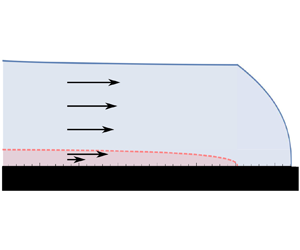
We consider the gravity-driven flow of two superposed thin films of viscous fluid of different physical properties, spreading over a horizontal substrate as illustrated in the schematic of figure 1. We assume that the two viscous fluids are immiscible, and that the effects of inertia and surface tension between the two layers are negligible. We use lubrication theory to develop a mathematical model of the flow by balancing viscous and buoyancy forces, assuming that vertical shear stresses provide the dominant resistance to the flow. The flow consists of a lubricated region, in which one layer of fluid intrudes beneath another, and a no-slip region, beyond the intrusion front of the underlying layer. The position of the intrusion front, or lubrication front, is denoted by  $\boldsymbol {x}=\boldsymbol {x_L}$, while the position of the leading edge of the no-slip current is denoted by $\boldsymbol {x}=\boldsymbol {x_N}$. The upper surface is denoted by $z=H(\boldsymbol {x},t)$ for the upper layer and $z=h(\boldsymbol {x},t)$ for the lower layer. The velocity field within the upper and lower layers are denoted by $\boldsymbol {u}$ and $\boldsymbol {u_l}$, respectively.

Figure 1. Schematic of the flow of two superposed thin films of power-law viscous fluids spreading under gravity over a horizontal substrate in a two-dimensional geometry. Schematic adapted from Kowal & Worster (Reference Kowal and Worster2015).
The two layers are of different viscosities  $\mu$ and $\mu _l$ and densities $\rho$ and $\rho _l$, where the subscript $_l$ denotes quantities related to the lower layer. We assume that both films of fluid follow a non-Newtonian, power-law rheology, also known as the Ostwald-de Waele power law, so that
 \begin{equation} \mu = \tilde \mu \left|\frac{\partial \boldsymbol u}{\partial z}\right|^{{1}/{n}-1},\quad \mu_l = \tilde \mu_l \left|\frac{\partial \boldsymbol u_l}{\partial z}\right|^{{1}/{n_l}-1}, \end{equation}
within the limits of lubrication theory, where  $\tilde \mu$ and $\tilde \mu _l$ are constant. We derive governing equations for equal power-law exponents ( $n= n_l$) and note that unequal exponents ( $n\neq n_l$) set an intrinsic length scale for the flow, which precludes self-similarity. This can be seen by considering the flow of a single-layer viscous gravity current of a power-law fluid, in two configurations, each of which involves a different viscous fluid of a different power-law exponent. The flows in each of these configurations are self-similar (Sayag & Worster Reference Sayag and Worster2013), and the leading edges of these flows propagate at a rate given by a time-dependent power law of different exponents. Balancing these (time-dependent) similarity length scales of these two flows gives rise to a characteristic length and time scale at which the spreading of the two fluids balances had they been superposed. Exact expressions for this length scale are presented in § 3 in two geometries. However, when $n=n_l$, no such length scale emerges (it can be seen that the said length scale diverges) and the systems tend towards a self-similar flow at late times starting from various initial conditions, similar to what has been demonstrated for single-layer viscous gravity currents (Ball & Huppert Reference Ball and Huppert2019). We focus on self-similar flows in the analysis of this paper and the companion paper. These correspond to the flows of Kowal & Worster (Reference Kowal and Worster2015) in the long-time limit for $n=1$.
We examine the flow in two geometrical settings: (i) a two-dimensional geometry, in which both layers of fluid spread unidirectionally with no cross-flow variations (so that the flow is uniform in the cross-flow variable  $y$); and (ii) an axisymmetric geometry, in which both layers of fluid spread radially outward from a specified origin, with no azimuthal variations (so that the flow is uniform in the azimuthal variable $\theta$). Both layers of fluid are supplied at constant line flux at $x=0$, denoted by $q_0$ for the upper layer and $q_{l0}$ for the lower layer in the two-dimensional setting, and at constant point flux at the origin, denoted by $Q_0$ for the upper layer and $Q_{l0}$ for the lower layer in the axisymmetric setting.
In terms of applications to the geophysical scenario of ice lubricated by meltwater-saturated till, we note that the source flux conditions are merely an idealisation for mathematical convenience. Realistically, the accumulation of both layers is actually distributed throughout the domain, with ice accumulation resulting from net snowfall minus melting over the whole domain, and till accumulation resulting from traction and bed failure over the whole domain, with locally distributed water sources from drainage of supraglacial meltwater down crevasses and other water outlets to the bottom of the ice, along with a distributed water source from basal melting throughout the domain. We have idealised both distributed processes as a point source, which is an idealisation necessary for the emergence of similarity solutions, rather than one that directly reflects actual geophysical settings.
For brevity, we derive the governing equations for both geometries simultaneously. To do so, we denote the partial derivates  $\partial h/\partial x$ and $\partial H/\partial x$, in the two-dimensional setting, and the partial derivatives $\partial h/\partial r$ and $\partial H/\partial r$, in the axisymmetric setting, collectively by $\delta h$ and $\delta H$, for compactness. We define the horizontal velocities, $\boldsymbol u$ and $\boldsymbol {u_l}$, and depth-integrated fluxes, $\boldsymbol q$ and $\boldsymbol {q_l}$, of the upper and lower layers, respectively, and the position of the lubrication front $\boldsymbol x=\boldsymbol {x_L}$ and leading edge $\boldsymbol x=\boldsymbol {x_N}$ as
 \begin{equation} \boldsymbol u = u \boldsymbol{e_x}, \quad \boldsymbol{u_l} = {u_l} \boldsymbol{e_x}, \quad \boldsymbol q = q \boldsymbol{e_x}, \quad \boldsymbol{q_l} = {q_l} \boldsymbol{e_x}, \quad \boldsymbol{x_L} = x_L \boldsymbol{e_x}, \quad \boldsymbol{x_N} = x_N \boldsymbol{e_x}, \end{equation}
in the two-dimensional setting, where  $\boldsymbol {e_x}$ is the unit basis vector defining the positive $x$ direction. Similarly, in the axisymmetric setting, we define these quantities as
 \begin{equation} \boldsymbol u = u \boldsymbol{e_r}, \quad \boldsymbol{u_l} = {u_l} \boldsymbol{e_r}, \quad \boldsymbol q = q \boldsymbol{e_r}, \quad \boldsymbol{q_l} = {q_l} \boldsymbol{e_r}, \quad \boldsymbol{x_L} = r_L \boldsymbol{e_r}, \quad \boldsymbol{x_N} = r_N \boldsymbol{e_r}, \end{equation}
where  $\boldsymbol {e_r}$ is the unit basis vector defining the radially outward direction.
2.1. Lubricated region
A horizontal force balance under the approximations of lubrication theory gives
 $$\begin{gather} \frac{\partial}{\partial z}\left(\mu \frac{\partial \boldsymbol u}{\partial z}\right) = \rho g\boldsymbol{\nabla} H, \quad h< z< H, \end{gather}$$
 $$\begin{gather}\frac{\partial}{\partial z}\left(\mu_l \frac{\partial \boldsymbol u_l}{\partial z}\right) = \rho g(\mathcal{D}\boldsymbol{\nabla} h+\boldsymbol{\nabla} H), \quad 0< z< h, \end{gather}$$
for the two thin films of fluid, where the pressure is hydrostatic to leading order,
 $$\begin{gather} p= p_0 +\rho g(H-z) \quad \text{for}\ h< z< H, \end{gather}$$
 $$\begin{gather}p_l = p_0 +\rho g(H-h)+\rho_lg(h-z) \quad \text{for}\ 0< z< h. \end{gather}$$
Apart from the power-law exponents  $n$ and $n_l$, which we assume to be equal, the governing equations depend on the dimensionless density difference $\mathcal {D}$ and consistency ratio $\mathcal {M}$, and flux ratio $\mathcal {Q}$ defined by
 \begin{equation} \mathcal{D} = \frac{\rho_l-\rho}{\rho}, \quad \mathcal{M} = \frac{\tilde \mu}{\tilde \mu_l}, \quad \mathcal{Q} = \frac{q_{l0}}{q_{0}}. \end{equation}
The above definition of  $\mathcal {Q}$ holds for the two-dimensional geometry. In the axisymmetric geometry, it is given by $\mathcal {Q} = {Q_{l0}}/{Q_{0}}$.
Integrating (2.4)–(2.5) describing the horizontal force balance, subject to the no-slip boundary condition at  $z=0$, continuity of velocity and shear stress at $z=h$, and the no-stress condition at the upper surface $z=H$, yields the following expressions for the horizontal velocities of the upper and lower layers,
 \begin{align} u &= \frac{1}{n+1}\left(\frac{\rho g}{\tilde \mu_l}\right)^{n} \frac{1}{\mathcal{D}\delta h+\delta H}[\left|(H-h)\delta H\right|^{n+1} -\left|h(\mathcal{D}\delta h+\delta H)+(H-h)\delta H\right|^{n+1}] \nonumber\\ &\quad +\frac{1}{n+1}\left(\frac{\rho g}{\tilde \mu}\right)^n [(H-z)^{n+1} - (H-h)^{n+1}] |\delta H|^{n-1} \delta H, \end{align}
and
 \begin{align} u_l&=\frac{1}{n+1}\left(\frac{\rho g}{\tilde \mu_l}\right)^{n} \frac{1}{\mathcal{D}\delta h+\delta H} [\left|(h-z)(\mathcal{D}\delta h+\delta H)+(H-h)\delta H\right|^{n+1}\nonumber\\ &\quad -\left|h(\mathcal{D}\delta h+\delta H)+(H-h)\delta H\right|^{n+1}], \end{align}
respectively.
Integrating across the depth of the upper layer of the lubricated region gives the following expression for the depth-integrated flux of fluid in the upper layer,
 \begin{align} q &= \frac{1}{n+1}\left(\frac{\rho g \mathcal{M}}{\tilde \mu}\right)^{n} \frac{H-h}{\mathcal{D}\delta h+\delta H} \left[\left|(H-h)\delta H\Big|^{n+1} - \Big|h(\mathcal{D}\delta h+\delta H) +(H-h)\delta H\right|^{n+1}\right] \nonumber\\ &\quad -\frac{1}{n+2} \left(\frac{\rho g}{\tilde \mu}\right)^n (H-h)^{n+2} |\delta H|^{n-1}\delta H, \end{align}
comprising Couette terms arising from viscous coupling with the lower layer and Poiseuille terms arising from gravitational spreading under its own weight. In the lower layer, the depth-integrated flux is given by
 \begin{align} q_l &= \frac{1}{n+1}\left(\frac{\rho g\mathcal{M}}{\tilde \mu}\right)^{n} \frac{1}{\mathcal{D}\delta h+\delta H}\left[-\frac{1}{n+2}\frac{1}{\mathcal{D}\delta h+\delta H} \left[\left|(H-h)\delta H\right|^{n+1} (H-h)\delta H \right.\right.\nonumber\\ &\quad \left.-\left|h(\mathcal{D}\delta h+\delta H)+(H-h)\delta H\right|^{n+1} (h(\mathcal{D}\delta h+\delta H)+(H-h)\delta H)\right] \nonumber\\ &\quad \left.\vphantom{\frac{1}{n+2}\frac{1}{\mathcal{D}\delta h+\delta H}} -h\left|h(\mathcal{D}\delta h+\delta H)+(H-h)\delta H\right|^{n+1}\right], \end{align}
comprising viscous coupling terms as well as terms arising from the spreading of the lower layer under its own weight and the weight of the overlying layer of fluid.
The evolution of the thickness of the two films of fluid is determined by the mass conservation equations
 \begin{equation} \frac{\partial (H-h)}{\partial t} ={-}\boldsymbol{\nabla}\boldsymbol{\cdot} \boldsymbol q, \quad \frac{\partial h}{\partial t} ={-}\boldsymbol{\nabla}\boldsymbol{\cdot}\boldsymbol{q_l}, \end{equation}
in the lubricated region.
2.2. No-slip region
In the no-slip region, the horizontal velocity and depth-integrated flux reduce to
 \begin{equation} u=\frac{1}{n+1}\left(\frac{\rho g}{\tilde \mu}\right)^n [(H-z)^{n+1} - (H)^{n+1}] |\delta H|^{n-1} \delta H, \end{equation}
and
 \begin{equation} q={-}\frac{1}{n+2} \left(\frac{\rho g}{\tilde \mu}\right)^n H^{n+2} |\delta H|^{n-1}\delta H. \end{equation}
The thickness of the thin film of fluid in the no-slip region is determined from the mass conservation equation
 \begin{equation} \frac{\partial H}{\partial t} ={-}\boldsymbol{\nabla}\boldsymbol{\cdot} \boldsymbol q. \end{equation}
These may be obtained by setting  $h=0$ in the expressions relevant to the lubricated region, serving as a way to double check the correctness of the equations derived for the lubricated region. These agree with the governing equations describing classical viscous gravity currents of power-law fluids, spreading axisymmetrically (Sayag & Worster Reference Sayag and Worster2013).
2.3. Boundary conditions
The governing equations are supplemented by the condition of continuity of flux
 \begin{equation} [\boldsymbol{q}\boldsymbol{\cdot} \boldsymbol{n}_{\boldsymbol{L}} + \boldsymbol{q}_{\boldsymbol{l}}\boldsymbol{\cdot} \boldsymbol{n}_{\boldsymbol{L}}]^- =[\boldsymbol{q}\boldsymbol{\cdot} \boldsymbol{n}_{\boldsymbol{L}}]^+ \quad \text{at}\ \boldsymbol x = \boldsymbol{x_L} \end{equation}
and thickness
 \begin{equation} [H]^- =[H]^+ \quad \text{at}\ \boldsymbol x = \boldsymbol{x_L} \end{equation}
across the lubrication front, where  $\boldsymbol x=\boldsymbol {x_L}$ is a vector describing the position of the lubrication front and $\boldsymbol {n_L}$ is the outward normal at the lubrication front.
Both fronts evolve kinematically,
 \begin{equation} \boldsymbol{n}_{\boldsymbol{L}} \boldsymbol{\cdot} \dot{\boldsymbol{x}}_{\boldsymbol{L}} = \lim_{\boldsymbol x\to \boldsymbol{x}_{\boldsymbol{L}}} \frac{\boldsymbol{n}_{\boldsymbol{L}} \boldsymbol{\cdot} \boldsymbol{q}_{\boldsymbol{l}}}{h}, \quad \boldsymbol{n}_{\boldsymbol{N}} \boldsymbol{\cdot} \dot{\boldsymbol{x}}_{\boldsymbol{N}} = \lim_{\boldsymbol x\to \boldsymbol{x}_{\boldsymbol{N}}} \frac{\boldsymbol{n}_{\boldsymbol{N}} \boldsymbol{\cdot} \boldsymbol{q}}{H}. \end{equation}
The normal component of the flux of the upper layer vanishes at the leading edge of the no-slip current, so that
 \begin{equation} \boldsymbol{q}\boldsymbol{\cdot} \boldsymbol{n}_{\boldsymbol{N}} = 0 \quad \text{at}\ \boldsymbol x = \boldsymbol{x_N}. \end{equation}
In contrast, the analogous condition
 \begin{equation} \boldsymbol{q}_{\boldsymbol{l}}\boldsymbol{\cdot} \boldsymbol{n}_{\boldsymbol{L}} = 0 \quad \text{at}\ \boldsymbol x = \boldsymbol{x_L}, \end{equation}
at the lubrication front holds if and only if  $\mathcal {D}\neq 0$. In the special case of the equal density limit ( $\mathcal {D}=0$), the stress singularity at the lubrication front reduces to a jump discontinuity, at which the lubrication front ends abruptly with a non-zero thickness (see Kowal & Worster Reference Kowal and Worster2015).
What remains to specify are the boundary conditions at the source, at which we assume a constant flux. This type of boundary condition depends on the geometry. In the two-dimensional setting, the two thin films of fluid are supplied at constant flux at the line source  $x=0$,
 \begin{equation} q=q_0, \quad q_l=q_{l0}, \quad\text{at}\ x=0, \end{equation}
while in the axisymmetric setting, the two fluids are supplied at constant flux at the point source  $r=0$,
 \begin{equation} \lim_{r\to0} 2{\rm \pi} r q=Q_0, \quad \lim_{r\to0} 2{\rm \pi} r q_l=Q_{l0}. \end{equation}
It is the dimensional differences in these boundary conditions that leads to different scaling laws for the flow in the two geometrical settings, determined in § 3.
The governing equations and boundary conditions specified here are sufficient to specify the flow completely. In the Newtonian limit ( $n=n_l=1$), these reduce to the governing equations and boundary conditions obtained by Kowal & Worster (Reference Kowal and Worster2015).
3. Similarity solutions
We lead the theoretical development by considering axisymmetric flows, and refer the reader to Appendix A for two-dimensional flows. We consider small perturbations to axisymmetric flows in Part 2.
3.1. Axisymmetric flows
At late times, a radially spreading lubricated viscous gravity current, for which  $n=n_l$, tends towards a self-similar flow, for which the thicknesses of the two layers scale as
 \begin{equation} \left(h(r,t), H(r,t)\right)=\left(\frac{\rho g}{\tilde \mu}\right)^at^bQ_0^c\cdot(f(\xi),F(\xi)) \end{equation}
in terms of the similarity variable  $\xi$, which we define in terms of the relationships
 $$\begin{gather} r = \left(\frac{\rho g}{\tilde \mu}\right)^\alpha t^\beta Q_0^\gamma \xi \xi_L \quad \text{for}\ 0< r< r_L, \end{gather}$$
 $$\begin{gather}r = \left(\frac{\rho g}{\tilde \mu}\right)^\alpha t^\beta Q_0^\gamma [\xi_L+(\xi-1)(\xi_N-\xi_L)] \quad \text{for}\ r_L< r< r_N, \end{gather}$$
where  $\xi _L$ and $\xi _N$ specify the lubrication front $r=r_L$ and leading edge $r=r_N$, respectively. That is,
 \begin{equation} r_L = \left(\frac{\rho g}{\tilde \mu}\right)^\alpha t^\beta Q_0^\gamma \xi_L \quad \text{and} \quad r_N = \left(\frac{\rho g}{\tilde \mu}\right)^\alpha t^\beta Q_0^\gamma \xi_N. \end{equation}
Such a rescaling maps the lubricated region to  $\xi \in (0,1)$ and the no-slip region to $\xi \in (1,2)$. Here,
 $$\begin{gather} a={-}\frac{2n}{5n+3},\quad b=\frac{n-1}{5n+3},\quad c=\frac{n+1}{5n+3}, \end{gather}$$
 $$\begin{gather}\alpha =\frac{n}{5n+3},\quad \beta = \frac{2n+2}{5n+3},\quad \gamma=\frac{2n+1}{5n+3}. \end{gather}$$
These scalings are identical to those of single-layer viscous gravity currents of power-law fluids in an axisymmetric geometry (Sayag & Worster Reference Sayag and Worster2013). Similar similarity solutions are obtainable in the glaciological context, of isothermal ice sheets with a net accumulation (Bueler et al. Reference Bueler, Lingle, Kallen-Brown, Covey and Bowman2005).
For unequal exponents,  $n\neq n_l$, the front of each viscous fluid propagates at a power law of different exponent, meaning that one of the viscous layers may overtake (or ‘outstrip’) the other. There is a characteristic length scale after which this may happen. This can be found by balancing the above scalings for viscous fluids of differing fluid properties and unequal power-law exponents, giving rise to a radial length scale given by
 \begin{equation} r\sim \left(L^{N}L_l^{{-}N_l}\right)^{1/(N-N_l)}, \end{equation}
where
 $$\begin{gather} L=\left(\frac{\rho g}{\tilde \mu}\right)^{n/(5n+3)} Q_0^{(2n+1)/(5n+3)},\quad L_l=\left(\frac{\rho_l g}{\tilde \mu_l}\right)^{n_l/(5n_l+3)} Q_{l0}^{(2n_l+1)/(5n_l+3)}, \end{gather}$$
 $$\begin{gather}N= \frac{3n+2}{5n+3}, \quad N_l= \frac{3n_l+2}{5n_l+3}. \end{gather}$$
The exponent  $1/(N-N_l)$ defining this length scale diverges in the limit of equal power-law exponents ( $n=n_l$). That is, no intrinsic length scale exists when $n=n_l$, enabling a self-similar flow regime to exist in this limit.
Under these scaling laws, the governing equations in the lubricated region,  $0<\xi <1$, reduce to
 \begin{gather} q={-}\frac{\left(F-f\right){}^{n+2} \left| F'\right|^{n-1}F' }{(n+2)\xi _{L}^{n}} +\frac{\mathcal{M}^n\left(F-f\right) \left(\left| \left(F-f\right) F'\right| {}^{n+1}- \left|\mathcal{D} f f'+F F'\right| {}^{n+1}\right)}{(n+1) \xi _{L}^{n}\left(\mathcal{D} f'+F'\right)}, \end{gather}
 \begin{gather} \hspace{-2.3pc} q_{l} ={-}\frac{\mathcal{M}^n}{(n+1) (n+2)} \frac{1}{\xi_{L}^n}\frac{1}{\left(\mathcal{D}f'+F'\right)^2} [\left(F-f\right)^{n+2} \left| F'\right|^{n+1}F' \nonumber\\ +\left|\mathcal{D} f f'+F F'\right|^{n+1} ((n+1)f(\mathcal{D} f'+F')-(F-f) F')], \end{gather}
 $$\begin{gather} \frac{(n-1)}{5 n+3}f - \frac{2 (n+1)}{5 n+3} \xi f'={-} \frac{\left(\xi q_{l}\right)'}{\xi \xi_{L}} \end{gather}$$
 $$\begin{gather}\frac{n-1}{5 n+3}(F-f) -\frac{2 (n+1) }{5 n+3}\xi (F' - f') ={-}\frac{\left(\xi q\right)'}{\xi \xi_{L}}. \end{gather}$$
The first term of the expression (3.10) for  $q$ is a Poiseuille-like contribution originating from the gravitational spreading of the upper layer under its own weight, while the second term comprises a Couette-like viscous coupling contribution, induced by the motion of the lower layer. Similarly, the last term of the expression (3.11) for $q_l$ reflects a Poiseuille-like flow driven by the spreading of the film under its own weight and the weight of the fluid above it. The pressure gradient, driving the flow of the lower layer, depends on both surface heights in the presence of a non-zero density difference between the two layers. The first term is a Couette-like contribution induced by motion at the interface between the two layers.
In the no-slip region,  $1<\xi <2$,
 \begin{equation} q={-}\frac{F^{n+2}}{(n+2)}\frac{F'}{\left(\xi_{N}-\xi_{L}\right)} \left|\frac{F'}{\xi_{N}-\xi_{L}}\right|^{n-1}, \end{equation}
and
 \begin{align} & \frac{(n-1)}{5 n+3} F -\frac{2 (n+1) }{5 n+3} \left(\xi-1+\frac{\xi_L}{\xi_N-\xi_L}\right) F' \nonumber\\ &\quad =\frac{q }{ (\xi -2) \xi_{L}-(\xi -1) \xi_{N} } + \frac{ q' }{\xi_{L}-\xi_{N} }. \end{align}
The boundary conditions in similarity coordinates reduce to
 $$\begin{gather} \lim_{\xi\rightarrow0}2{\rm \pi}\xi_{L}\xi q = 1 \quad \text{and} \quad \lim_{\xi\rightarrow0}2{\rm \pi}\xi_{L}\xi q_{l} = \mathcal{Q}, \end{gather}$$
 $$\begin{gather}\left[ F \right]^+_- = 0 \quad \text{and}\quad \left[ q \right]^+_- = 0 \quad \text{at}\ \xi=1, \end{gather}$$
 $$\begin{gather}q_{l} = 0 \quad \text{at}\ \xi=1 \quad\text{if}\ \mathcal{D}\neq0, \end{gather}$$
 $$\begin{gather}q = 0 \quad \text{at}\ \xi=2, \end{gather}$$
and the kinematic conditions become
 \begin{equation} \frac{2n+2}{5n+3}\xi_{L} = \lim_{\xi\rightarrow1}\frac{q_{l}}{f} \quad \text{and} \quad \frac{2n+2}{5n+3}\xi_{N} = \lim_{\xi\rightarrow2}\frac{q}{F}. \end{equation}
3.2. Asymptotic solutions
The solutions involve singularities at the boundaries of the lubricated and no-slip regions. The singularities at the two fronts occur as a consequence of diverging stress at the nose of each current. These singularities occur in both geometries. A secondary singularity at the origin occurs for radially spreading flows as a consequence of a finite amount of fluid being supplied at a single point.
The presence of these singularities prompt the need for asymptotic solutions at the end points in order to obtain robust numerical solutions within the whole domain.
We present asymptotic results in the axisymmetric configuration in this section, and refer the reader to Appendix A for asymptotic solutions in the two-dimensional configuration.
3.2.1. Asymptotic solution near the fronts
An asymptotic analysis near the lubrication front in the axisymmetric geometry reveals the asymptotic solution
 \begin{equation} f \sim\left[\frac{2(n+1) (n+2) \xi_{L}}{5 n+3} \left(\frac{(2 n+1) \xi_{L}}{\mathcal{M} \mathcal{D} n}\right)^n \right]^{{1}/{(2n+1})}(1-\xi )^{n/(2 n+1)} \quad \text{as}\ \xi\to1, \end{equation}
in the lubricated region near the intrusion front and the asymptotic solution
 \begin{align} F \sim \left[\frac{ 2\left(n+1\right)\left(n+2\right) \xi_{N} }{ 5 n+3 } \left(\frac{(2n+1)(\xi_{N}-\xi_{L})}{n}\right)^{n} \right]^{{1}/{(2 n+1)}}(2-\xi )^{{n}/{(2 n+1)}} \quad \text{as}\ \xi\to2, \end{align}
near the leading edge. These satisfy the kinematic conditions and the governing equations near the two fronts.
These asymptotic solutions are shown in figure 2 in both geometrical settings (see Appendix A for asymptotic solutions in the two-dimensional geometry). A lesser agreement between the asymptotic solution and the full similarity solution is seen near the lubrication front, as forces other than the buoyancy forces associated with the lower layer are driving the flow of the lower layer, away from the lubrication front. However, the agreement becomes better as the lubrication front is approached.
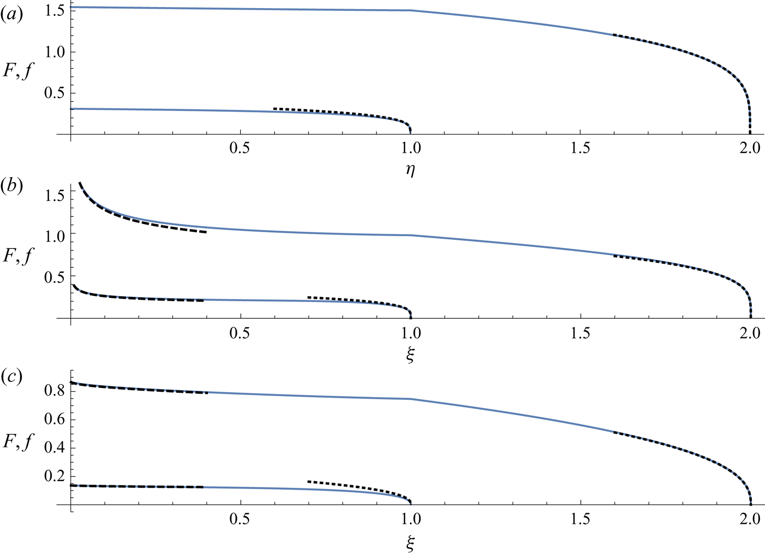
Figure 2. Asymptotic solutions (3.21)–(3.22) and (A21)–(A22) (dotted curves) near the two fronts in similarity coordinates in comparison to the full similarity solution (solid curves) for the profile thicknesses  $f$ and $F$ of the two layers in the two-dimensional (a) and axisymmetric (b,c) settings. Asymptotic solutions (3.24) for $n<1$ (dashed curves, b) and (3.23) for $n>1$ (dashed curves, c) depicting the singularity near the origin for the axisymmetric problem are shown near the origin. Parameters used: $\mathcal {M}=20$, $\mathcal {D}=2$, $\mathcal {Q}=0.1$ (a–c), $n=1/2$ (a,b) and $n=2$ (c).
The region of validity, in which the asymptotic solution remains valid, in  $\eta$, is largest for small values of $n$, indicating that buoyancy forces associated with the lower layer are most dominant for small values of $n$. As $n$ increases, other forces become increasingly dominant.
The asymptotic solution shows that the frontal singularities become more pronounced the more shear thickening the flow, as shown illustratively in figure 3 for the asymptotic solution near the lubrication front. Gradients near the lubrication front become increasingly steep the lower the value of  $n$, leading to a near-vertical front for low $n$.
$n$.

Figure 3. Asymptotic solution (A21) in similarity coordinates for the lower layer in the two-dimensional geometry for various values of  $n$. The frontal singularity becomes more pronounced for shear-thickening flows. Parameters used: $\mathcal {M}=20$, $\mathcal {D}=2$, $\mathcal {Q}=0.1$ and $n=1/10$, $1$, and $10$.
$10$.
3.2.2. Asymptotic solution near the origin
The solutions to the governing equations become asymptotically large near the origin for radially spreading flows and the character of the singularity depends on the value of  $n$. In the Newtonian case, the solutions involve a weak logarithmic singularity near the origin as seen in Huppert (Reference Huppert1982) and Kowal & Worster (Reference Kowal and Worster2015).
The singularity sharpens for shear-thinning flows ( $n>1$), for which the slopes of the two films of fluid diverge as
 \begin{equation} (F,f) \sim (\mathcal{A},\mathcal{a}) (1+v \xi ^{1-{1}/{n}})^{{n}/{(2 n+2)}}\quad \text{as}\ \xi\to0 \end{equation}
to leading order, where  $\mathcal {A}$, $\mathcal {a}$ and $v$ are constants.
For shear-thickening flows ( $n<1$), the thicknesses of the two layers diverge as
 \begin{equation} (F, f) \sim (\mathcal{B},\mathcal{b}) \xi^{-({(1-n)}/{2 (n+1)})} \quad \text{as}\ \xi\to0, \end{equation}
where  $\mathcal {B}$ and $\mathcal {b}$ are constants that diverge as $(1-n)^{-n/(2n+2)}$ as $n\to 1^-$. The coefficients describing these asymptotic solutions satisfy the system of equations outlined in Appendix B. There is no closed-form solution for this nonlinear system, in general.
The asymptotic solutions (3.23) for  $n>1$ and (3.24) for $n<1$ are plotted against the full numerical solution in figure 2.
3.3. Numerical solutions
We use the approach adopted by Kowal & Worster (Reference Kowal and Worster2015) to integrate the governing equations numerically. In particular, the governing equations have been solved over the interval  $(0,\ 1-\delta )$ for the lubricated region, and $(1,\ 2-\delta )$ for the no-slip region, where $\delta \ll 1$ is a small parameter, in the two-dimensional configuration. In the axisymmetric configuration, the equations modelling the lubricated region have instead been solved over the smaller interval $(\varDelta,\ 1-\delta )$, owing to the weak singularity at the origin, where $\varDelta \ll 1$.
The asymptotic solutions (3.21)–(3.22) and (A21)–(A22) have been used in the small intervals  $(1-\delta, 1]$ and $(2-\delta, 2]$, and as boundary conditions specifying the layer thickness and slope at $\xi =1-\delta$ and $\xi =2-\delta$ in the axisymmetric configuration and at $\eta =1-\delta$ and $\eta =2-\delta$ in the two-dimensional configuration. We do so by shooting backwards from the leading edge $\xi =2$ in the axisymmetric geometry and $\eta =2$ in the two-dimensional geometry, with $\xi _L$ and $\xi _N$ (respectively, $\eta _L$ and $\eta _N$) being shooting parameters. That is, $\xi _L$ and $\xi _N$ (respectively, $\eta _L$ and $\eta _N$) are found as part of the numerical solution. The numerical integration has been implemented in Mathematica and the numerical solutions have been validated by confirming agreement with those of Kowal & Worster (Reference Kowal and Worster2015) for $n=1$, and with the asymptotic solutions (3.21)–(3.22) and (A21)–(A22) for a range of values of $\delta$ and $\varDelta$.
Figure 2 displays both the full numerical solution over the interval  $[0,1-\delta ]$, and the frontal asymptotic solutions over the interval $[0.7,1]$, which extends beyond its region of validity, for completeness, in the two geometries.
4. Flow regimes
The similarity solutions derived in the prior sections depend upon four dimensionless parameters, namely: the consistency ratio  $\mathcal {M}$, the density difference $\mathcal {D}$, the flux ratio $\mathcal {Q}$ and the power-law exponent $n$. The behaviour of the flow, and the mechanisms driving the flow, are sensitive to the values of these parameters. In what follows, we assume that $\mathcal {D}$ is a fixed value bounded away from zero and we investigate the emerging flow regimes in $(\mathcal {Q}, \mathcal {M})$ parameter space.
Akin to the results of Kowal & Worster (Reference Kowal and Worster2015), the flow can be categorised into four distinct flow regimes, which we label using roman numerals as described in table 1. Regime diagrams depicting the four regimes in the two-dimensional and axisymmetric geometries are shown in figure 4 for various values of  $n$, which we refer to in the discussion, below. The curves depicting the boundaries between the regimes are obtained numerically based on the criteria summarised in table 1, as there are no explicit formulae for these in general. The results of this section reduce to those obtained by Kowal & Worster (Reference Kowal and Worster2015) in the limit of $n=1$, though the correspondence is less clear for the boundary between regimes II and III. It should be noted that the definitions of the regime boundaries in Kowal & Worster (Reference Kowal and Worster2015) are indicative order-of-magnitude estimates only, rather than quantitative as is the case here.

Figure 4. Regime diagram in  $(\mathcal {Q},\mathcal {M})$-space for $\mathcal {D}=1$ and $n=1/2,1,2$ in the two-dimensional (a) and axisymmetric (b) settings. The red curves are contours of $\zeta _L=\zeta _N-\zeta _L$ and the blue curves are contours of $\bar f=\bar F-\bar f$, separating regimes I–IV as outlined in table 1.
Table 1. Summary of parameter regimes.

We lead the discussion by example of axisymmetric flows and present abbreviated results for two-dimensional flows in Appendix A. In what follows, we summarise the leading-order equations for both geometries simultaneously. For brevity, we denote  $\eta _L$ and $\eta _N$, for two-dimensional flows, and $\xi _L$ and $\xi _N$, for axisymmetric flows, collectively by $\zeta _L$ and $\zeta _N$, respectively.
4.1. Regime I: classical spreading of the overlying layer
Regime I is one in which the upper layer spreads gravitationally under its own weight, largely unaffected by the underlying layer, and the motion generated at the interface induces a shear flow within the underlying layer. Such a balance of forces results in the following leading-order contributions
 $$\begin{gather} q_l={-}\frac{\mathcal{M}^n}{2\zeta_L^{n}} f^2 F^n \left| F'\right|^{n-1}F', \end{gather}$$
 $$\begin{gather}q={-}\frac{1}{(n+2) \zeta_L^n}F^{n+2} F' \left| F'\right| ^{n-1} \end{gather}$$
to the fluxes of the two layers of fluid. These can be deduced by reference to the physical description of the terms comprising the fluxes of the two layers, described in the paragraph following (3.11), and by noting that  $F\gg f$. In this case, the lubricated region is relatively thin with a short extent, and its effect on the upper layer is small. The flow of the upper layer is similar to that of a classical viscous gravity current of a single layer of fluid spreading over a rigid, no-slip surface.
For the purposes of the illustration of figure 4, we define this regime quantitatively as one in which
 \begin{equation} \bar f < \bar F-\bar f, \quad \zeta_L<\zeta_N-\zeta_L, \end{equation}
where  $\bar f$ and $\bar F$ are the average lower and upper layer thicknesses, respectively, over the lubricated region. These are defined by
 \begin{equation} \bar f = \int_0^{1} f(\eta)\,{\rm d}\eta \end{equation}
in the two-dimensional configuration and
 \begin{equation} \bar f = \int_0^{1} 2 f(\xi)\xi\,{\rm d}\xi \end{equation}
in the axisymmetric configuration, and similarly for  $\bar F$.
The remaining part of parameter space is covered by three further parameter regimes, defined in terms of similar inequalities discussed in the subsequent subsections. To compute the boundaries of these regions of parameter space, we replace the two inequalities of (4.3a,b) by corresponding equalities and search for the parameter  $\mathcal {M}$ for which the first equality is satisfied (as a function of the remaining parameters) to obtain one of the curves of figure 4 defining the boundary, and repeat for the second equality to obtain the other curve. Regions in between these curves correspond to the four parameter regimes discussed in this section.
Flows corresponding to this regime occur for low values of  $\mathcal {Q}$ and intermediate values of $\mathcal {M}$ as shown in the regime diagram of figure 4. It can be seen from the regime diagram that the region of parameter space corresponding to regime I reduces with increasing values of $n$ – both the upper and lower boundaries of this region contract.
Typical profile thicknesses of axisymmetric lubricated viscous gravity currents under regime I are depicted in figure 7. As the lubricating layer becomes very thin in this regime, we have taken  $\mathcal {M}=1$ for visibility. The lubricating layer thins and extends and the overlying layer flattens as $n$ increases. The shape of the overlying current is largely unchanged by the presence of the lower layer. The average thickness and frontal positions are displayed in figure 5, transitioning from regime I for small $\mathcal {Q}$ towards regimes III and II for large $\mathcal {Q}$, for various values of $n$, and in figure 6 as a function of $n$. Increasing $n$ promotes the thinning and elongating of both layers. This may be a consequence of shear-thinning currents being thinner and longer than shear-thickening currents, in general.

Figure 5. (a) The average surface heights of the upper and lower layers (solid and dashed curves, respectively) in similarity coordinates in the axisymmetric setting vs  $\mathcal {Q}$. (b) The frontal positions $\xi =\xi _N$ and $\xi _L$ (solid and dashed curves, respectively) in the axisymmetric setting vs $\mathcal {Q}$. Parameters used: $\mathcal {M} = 50$, $\mathcal {D} =1$ and $n=1/2,1,2$.

Figure 6. (a) The average upper surface height of the upper and lower layers (solid and dashed curves, respectively) in similarity coordinates in the axisymmetric setting vs  $n$. (b) The frontal positions $\xi =\xi _N$ and $\xi _L$ (solid and dashed curves, respectively) in the axisymmetric setting vs $n$. Parameters used: $\mathcal {M} = 5$, $\mathcal {D} = 1$, $\mathcal {Q}= 0.1$.

Figure 7. Profile thicknesses  $f$ and $F$ of axisymmetric lubricated viscous gravity currents falling under regime I for $\mathcal {M}=1$, $\mathcal {D}=1$, $\mathcal {Q}=0.05$ and $n=1/2$ (a), $n=1$ (b) and $n=2$ (c). The thicknesses of the overlying and underlying layers are given by the solid and dashed curves, respectively.
4.2. Regime II: flow driven by the underlying layer
Under regime II, the motion is driven by the lower layer, which is spreading gravitationally under its own weight and the weight of the fluid above it. The flow of the overlying layer is driven by interfacial stresses between the two layers. Effectively, the lower layer pulls the upper layer along with it, which behaves like a plug-like flow. Such a balance results in the leading-order contributions
 $$\begin{gather} q_l={-}\frac{\mathcal{M}^n(\mathcal{D}+1)^n }{(n+2) \zeta_L^n}f^{n+2} \left| f'\right| ^{n-1}f', \end{gather}$$
 $$\begin{gather}q={-}\frac{\mathcal{M}^n(\mathcal{D}+1)^n }{(n+1) \zeta_L^n}(F-f) f^{n+1} \left| f'\right| ^{n-1}f', \end{gather}$$
to the fluxes of fluid in the two layers. Both of these involve gradients in the lower layer thickness only. These can be deduced by reference to the physical description of the terms comprising the fluxes of the two layers, described in the paragraph following (3.11), and by noting that  $f\gg F-f$.
A consequence is that gradients in the upper layer surface height are not influential to leading order and slope reversals in the upper surface height can occur, as shown in figure 8. Figure 8 shows typical profile thicknesses for  $n<1$, $n=1$ and $n>1$. A slope reversal near the lubrication front occurs in all three cases, although in reduced form for $n>1$. Despite the reversed slope of the upper surface height near the lubrication front, which gives rise to a negative contribution to the flux of fluid in the upper layer, the dominant contribution to the flow of the upper layer originates from the motion of the lower layer, which is downstream.

Figure 8. Profile thicknesses  $f$ and $F$ of axisymmetric lubricated viscous gravity currents falling under regime II for $\mathcal {M}=100$, $\mathcal {D}=1$, $\mathcal {Q}=2$ and $n=1/2$ (a), $n=1$ (b) and $n=2$ (c). The thicknesses of the overlying and underlying layers are given by the solid and dashed curves, respectively.
These slope reversals are most prominent for  $n<1$. Increasing $n$ thins and elongates both layers, as seen for the other regimes, and as seen in the plots of the average thickness and frontal positions in figure 5. As mentioned earlier, this may be a consequence of shear-thinning currents being thinner and longer than shear-thickening currents, in general. A prominent feature that occurs for increasing values of $n$ is the increasing thinning of the overlying layer, which behaves like a viscous coating over the underlying layer of fluid, which is driving the flow.
We define this regime quantitatively as one in which
 \begin{equation} \bar f > \bar F-\bar f, \quad \zeta_L>\zeta_N-\zeta_L. \end{equation}
As seen in the regime diagrams of figure 4, the flows of regime II occur for large values of the flux ratio  $\mathcal {Q}$ and moderate values of the consistency ratio $\mathcal {M}$. This means that the overlying viscous coating may be either more or less viscous than the driving viscous gravity current. This regime occurs more frequently for small values of $n$. Increasing values of $n$ lead to a diminishing region of parameter space describing region II.
4.3. Regime III: thin lubricating layer
Regime III characterises itself by a thin lubricating layer, or a shear layer, to which most of the shear of the system is confined to. Despite its thinness, its presence significantly alters the dynamics of the overlying layer, which, in this regime, behaves like a plug flow. The thin lubricating shear layer deforms under hydrostatic pressure gradients associated with the upper layer. Even though these gradients are weak, the consistency ratio  $\mathcal {M}$ is large enough that the underlying, much less viscous layer is driven by these upper layer gradients.
This regime is unique in that the flow of neither layer is similar to that of a single-layer classical viscous gravity current consisting of a fluid with the properties of one or the other layer. The flow is significantly altered in both layers.
Such a balance results in the leading-order contributions
 $$\begin{gather} q_l={-}\frac{\mathcal{M}^n}{2 \zeta_L^n}f^2 F^n \left| F'\right| ^{n-1}F', \end{gather}$$
 $$\begin{gather}q={-}\frac{\mathcal{M}^n }{\zeta_L^n} f F^{n+1} \left| F'\right| ^{n-1}F', \end{gather}$$
to the fluxes of the two layers of fluid. Both of these involve gradients in the upper surface height of the overlying layer of fluid. These can be deduced by reference to the physical description of the terms comprising the fluxes of the two layers, described in the paragraph following (3.11), and by noting that  $f\ll F-f$.
We define this regime quantitatively as one in which
 \begin{equation} \bar f < \bar F-\bar f, \quad \zeta_L>\zeta_N-\zeta_L. \end{equation}
As seen in the regime diagrams of figure 4, the flows of regime III occur for large values of the consistency ratio  $\mathcal {M}$ and moderate values of the flux ratio $\mathcal {Q}$. Regime III becomes increasingly prominent for increasing values of $n$.
$n$.
Typical profile thicknesses of the two layers of fluid are shown in figure 9 for  $n<1$, $n=1$ and $n>1$. There is a visible flattening of the upper surface of the overlying layer of fluid, which becomes more apparent for $n>1$. There is a departure to this observation near the origin, at which there is a weak singularity. A similar observation can be made about the lubricating layer, apart from the vicinity of the lubrication front, at which the underlying layer spreads under its own weight owing to large thickness gradients of the underlying layer in this region.

Figure 9. Profile thicknesses  $f$ and $F$ of axisymmetric lubricated viscous gravity currents falling under regime III for $\mathcal {M}=100$, $\mathcal {D}=1$, $\mathcal {Q}=0.1$ and $n=1/2$ (a), $n=1$ (b) and $n=2$ (c). The thicknesses of the overlying and underlying layers are given by the solid and dashed curves, respectively.
Apart from this flattening, increasing values of  $n$ thin and elongate both layers of fluid, as seen in figure 9 and the plots of the average thickness and frontal positions in figure 5, corresponding to regime III. As mentioned earlier, this may follow from shear-thinning currents being thinner and longer than shear-thickening currents, in general.
4.4. Regime IV: low-viscosity thin film coating a more viscous current
Regime IV consists of flows driven mainly by the gravitational spreading of the underlying layer, which spreads mainly under its own weight with negligible influence of the overlying layer. The overlying layer behaves as a thin coating film of fluid, which exerts negligible shear stress on the underlying layer and provides little resistance to the flow. Such a balance results in the leading-order contributions
 $$\begin{gather} q_l={-}\frac{\mathcal{M}^n(\mathcal{D}+1)^n }{(n+2) \zeta_L^n}f^{n+2} \left| f'\right| ^{n-1}f', \end{gather}$$
 $$\begin{gather}q={-}\frac{1}{(n+2) \zeta_L^n} (F-f)^{n+2} \left| F'\right| ^{n-1}F', \end{gather}$$
to the fluxes of the two layers of fluid. These can be deduced by reference to the physical description of the terms comprising the fluxes of the two layers, described in the paragraph following (3.11), and by noting that  $f\gg F-f$.
In contrast to regime II, flows under regime IV do not involve upper surface slope reversals near the lubrication front, as the flow of the upper layer is driven by hydrostatic pressure gradients established within the overlying layer, rather than the underlying layer. The coupling between the two layers is purely a consequence of geometry, rather than dynamics.
Both this regime and regime III involve thin films of fluid – a thin coating layer, overlying the driving viscous gravity current in the case of regime IV, and a thin lubricating layer, underlying the driving viscous layer in the case of regime III. In contrast to regime III, the thin coating film exerts negligible shear stress on the driving layer as it is a coating covering the driving layer from above. A simple change in location of the film produces significant dynamical changes. That is, the flow changes significantly when the thin film is a lubricating film, underlying the driving layer from below as in regime III.
We define this regime quantitatively as one in which
 \begin{equation} \bar f > \bar F-\bar f, \quad \zeta_L<\zeta_N-\zeta_L. \end{equation}
Flows under regime IV occur for low consistency ratios and moderate flux ratios, as shown in figure 4. Such flows become increasingly common for increasing values of  $n$ – similarly to regime III.
Illustratively, such flows involve a low-viscosity thin film of fluid coating a more viscous layer. Plots of typical profile thicknesses of the two layers of fluid are shown in figure 10 for various values of  $n$. Slope reversals do not occur near the lubrication front and the overlying, less viscous layer freely runs out ahead of the front. The thin coating film becomes less noticeable, and runs ahead further, for increasing values of $n$.
$n$.

Figure 10. Profile thicknesses  $f$ and $F$ of axisymmetric lubricated viscous gravity currents falling under regime IV for $\mathcal {M}=0.005$, $\mathcal {D}=1$, $\mathcal {Q}=0.4$ and $n=1/2$ (a), $n=1$ (b) and $n=2$ (c). The thicknesses of the overlying and underlying layers are given by the solid and dashed curves, respectively.
5. Conclusions
We investigated the effect of shear-thinning and shear-thickening rheology on the flow of lubricated viscous gravity currents in self-similar form, both in a two-dimensional and in an axisymmetric geometry. Similarity solutions exist in both geometries as long as the power-law exponents, describing the rheology of the viscous fluids, are identical in both layers. Four distinct flow regimes emerge depending on the consistency ratio  $\mathcal {M}$, the density difference $\mathcal {D}$ and the flux ratio $\mathcal {Q}$. The flow regimes involve either (i) classical spreading of the overlying layer, largely unaffected by the underlying layer, in which the motion generated at the interface induces a shear flow within the underlying layer (regime I); (ii) a flow driven by the underlying layer, in which the interfacial stresses between the two layers drive a plug-like flow of the overlying layer (regime II); (iii) the flow of a thin lubricating layer, driven by hydrostatic pressure gradients associated with the upper layer, which, unlike its thinness, generates a plug flow within the overlying layer (regime III); and (iv) the flow of a low-viscosity thin film coating a more viscous current from above (regime IV).
Similar to purely Newtonian flows, a stress singularity is found at the nose of both layers of fluid for all power-law exponents. The frontal singularity becomes more pronounced the more shear thickening the rheology. Shear thickening leads to increasingly steep gradients near the two fronts, leading to the fronts becoming near vertical.
The flow dynamics is similar for shear thinning ( $n>1$), purely Newtonian ( $n=1$), and shear-thickening flows ( $n<1$) within each regime. However, the scalings, frontal positions, thicknesses, the structure of the singularity at the nose of both layers and the regime boundaries change intrinsically depending upon the rheology. Shear thinning, in general, promotes the elongating and thinning of both layers except when the overlying layer forms a low-viscosity thin film coating a more viscous current. This may be a consequence of shear-thinning currents being thinner and longer than shear-thickening currents, in general. As such, regimes III and IV become increasingly prominent for increasing values of the power-law exponent. The former regime, in which the main current is shear thinning and lubricated by a much less viscous thin layer of fluid from below, is most relevant to the flow of lubricated ice sheets and fast-flowing ice streams.

Figure 11. Profile thicknesses  $f$ and $F$ of two-dimensional lubricated viscous gravity currents falling under regime I for $\mathcal {M}=1$, $\mathcal {D}=1$, $\mathcal {Q}=0.05$ and $n=1/2$ (a), $n=1$ (b) and $n=2$ (c). The thicknesses of the overlying and underlying layers are given by the solid and dashed curves, respectively.

Figure 12. Profile thicknesses  $f$ and $F$ of two-dimensional lubricated viscous gravity currents falling under regime II for $\mathcal {M}=100$, $\mathcal {D}=1$, $\mathcal {Q}=2$ and $n=1/2$ (a), $n=1$ (b) and $n=2$ (c). The thicknesses of the overlying and underlying layers are given by the solid and dashed curves, respectively.

Figure 13. Profile thicknesses  $f$ and $F$ of two-dimensional lubricated viscous gravity currents falling under regime III for $\mathcal {M}=100$, $\mathcal {D}=1$, $\mathcal {Q}=0.1$ and $n=1/2$ (a), $n=1$ (b) and $n=2$ (c). The thicknesses of the overlying and underlying layers are given by the solid and dashed curves, respectively.

Figure 14. Profile thicknesses  $f$ and $F$ of two-dimensional lubricated viscous gravity currents falling under regime IV for $\mathcal {M}=0.005$, $\mathcal {D}=1$, $\mathcal {Q}=0.4$ and $n=1/2$ (a), $n=1$ (b) and $n=2$ (c). The thicknesses of the overlying and underlying layers are given by the solid and dashed curves, respectively.
Funding
L.T.L. acknowledges the support of a summer studentship through the Trinity College Summer Studentship Scheme. K.N.K. acknowledges funding through L'Oréal-UNESCO UK and Ireland, For Women In Science (FWIS).
Declaration of interests
The authors report no conflict of interest.
Data availability statement
The data that support the findings of this study are directly available within this publication.
Appendix A. Two-dimensional flows
At late times, a two-dimensional, lubricated viscous gravity current, for which  $n=n_l$, tends towards a similarity solution in which the thicknesses of the two layers scale as
 \begin{equation} \left(h(x,t), H(x,t)\right)=\left(\frac{\rho g}{\tilde \mu}\right)^at^bQ_0^c\cdot(f(\eta),F(\eta)) \end{equation}
in terms of the similarity variable  $\eta$, which we define in terms of the relationships
 $$\begin{gather} x = \left(\frac{\rho g}{\tilde \mu}\right)^\alpha t^\beta Q_0^\gamma \eta \eta_L \quad \text{for}\ 0< x< x_L, \end{gather}$$
 $$\begin{gather}x = \left(\frac{\rho g}{\tilde \mu}\right)^\alpha t^\beta Q_0^\gamma [\eta_L+(\eta-1)(\eta_N-\eta_L)] \quad \text{for}\ x_L< x< x_N, \end{gather}$$
where  $\eta _L$ and $\eta _N$ specify the lubrication front $x=x_L$ and leading edge $x=x_N$, respectively. That is,
 \begin{equation} x_L = \left(\frac{\rho g}{\tilde \mu}\right)^\alpha t^\beta Q_0^\gamma \eta_L \quad \text{and} \quad x_N = \left(\frac{\rho g}{\tilde \mu}\right)^\alpha t^\beta Q_0^\gamma \eta_N. \end{equation}
Such a rescaling maps the lubricated region to  $\eta \in (0,1)$ and the no-slip region to $\eta \in (1,2)$. Here,
 $$\begin{gather} a={-}\frac{n}{3n+2},\quad b=\frac{n}{3n+2}, \quad c=\frac{n+1}{3n+2}, \end{gather}$$
 $$\begin{gather}\alpha =\frac{n}{3n+2},\quad \beta = \frac{2n+2}{3n+2},\quad \gamma=\frac{2n+1}{3n+2}. \end{gather}$$
These scalings are identical to those of single-layer viscous gravity currents of power-law fluids in a two-dimensional geometry.
As for the axisymmetric problem, balancing these scalings for viscous fluids of differing fluid properties and unequal power-law exponents gives rise to a horizontal length scale given by
 \begin{equation} x\sim (L^{N}L_l^{{-}N_l})^{1/(N-N_l)}, \end{equation}
where
 $$\begin{gather} L=\left(\frac{\rho g}{\tilde \mu}\right)^{n/(3n+2)} Q_0^{(2n+2)/(3n+2)}, \quad L_l=\left(\frac{\rho_l g}{\tilde \mu_l}\right)^{n_l/(3n_l+2)} Q_{l0}^{(2n_l+2)/(3n_l+2)}, \end{gather}$$
 $$\begin{gather}N= \frac{3n+2}{2n+2}, \quad N_l= \frac{3n_l+2}{2n_l+2}. \end{gather}$$
Similarly as in the axisymmetric setting, the exponent  $1/(N-N_l)$ defining this length scale diverges in the limit of equal power-law exponents ( $n=n_l$), enabling a self-similar flow regime to exist in this limit.
Under these scaling laws, the governing equations for  $n=n_l$ in the lubricated region, $0<\eta <1$, reduce to
 \begin{gather} q={-}\frac{ \left(F-f\right){}^{n+2} \left| F'\right|^{n-1}F'}{(n+2)\eta _{L}^{n}} +\frac{ \mathcal{M}^n\left(F-f\right) \left(\left| \left(F-f\right) F'\right| {}^{n+1}- \left| \mathcal{D} f f'+F F'\right| {}^{n+1}\right)}{ (n+1) \eta _{L}^{n}\left(\mathcal{D} f'+F'\right)}, \end{gather}
 \begin{gather} \hspace{-2.2pc} q_{l}={-}\frac{\mathcal{M}^n}{(n+1) (n+2)}\frac{1}{\eta_{L}^n }\frac{1}{\left(\mathcal{D} f'+F'\right)^2}\left[ \left(F-f\right)^{n+2} \left| F'\right|^{n+1} F' \right. \nonumber\\ \left.+\left( (n+1)f \left(\mathcal{D} f'+F'\right)-\left(F-f\right) F' \right) \left|\mathcal{D} f f'+F F'\right|^{n+1} \right], \end{gather}
 $$\begin{gather} \frac{n}{3 n+2} f - \frac{2(n+1)}{3 n+2} \eta f'={-} \frac{ q_{l}'}{ \eta_{L}}, \end{gather}$$
 $$\begin{gather}\frac{ n}{3 n+2}(F-f) -\frac{2(n+1) }{3 n+2}\eta (F' - f') ={-}\frac{ q'}{ \eta_{L}}. \end{gather}$$
 In the no-slip region,  $1<\eta <2$,
 \begin{equation} q={-}\frac{ F^{n+2} }{ (n+2) }\frac{ F' }{\left(\eta_{N}-\eta_{L}\right) } \left|\frac{F'}{\eta_{N}-\eta_{L}}\right|^{n-1}, \end{equation}
and
 \begin{equation} \frac{n }{3n+2} F -\frac{2 (n+1) }{(3 n+2)} \left(\eta-1+\frac{\eta_L}{\eta_N-\eta_L}\right) F'={-}\frac{ q' }{ \eta_{N}-\eta_{L} }. \end{equation}
The boundary conditions in similarity coordinates reduce to
 $$\begin{gather} q = 1 \quad \text{and} \quad q_{l} = \mathcal{Q} \quad \text{at} \eta=0, \end{gather}$$
 $$\begin{gather}\left[ F \right]^+_- = 0 \quad \text{and} \quad \left[ q \right]^+_- = 0 \quad \text{at}\ \eta=1, \end{gather}$$
 $$\begin{gather}q_{l} = 0 \quad \text{at}\ \eta=1 \quad\text{if}\ \mathcal{D}\neq0, \end{gather}$$
 $$\begin{gather}q = 0 \quad \text{at}\ \eta=2, \end{gather}$$
and the kinematic conditions become
 \begin{equation} \frac{2n+2}{3n+2}\eta_{L} = \lim_{\eta\rightarrow1} \frac{q_{l}}{f} \quad \text{and} \quad \frac{2n+2}{3n+2}\eta_{N} = \lim_{\eta\rightarrow2}\frac{q}{F}. \end{equation}
A.1. Asymptotic solution near the fronts
An asymptotic analysis near the lubrication front in the two-dimensional geometry reveals the asymptotic solution
 \begin{equation} f \sim \left[\frac{2(n+1) (n+2) \eta_L}{3 n+2} \left(\frac{(2 n+1)\eta_L }{\mathcal{MD}n}\right)^n \right]^{{1}/{2 n+1}} (1-\eta )^{{n}/{(2 n+1)}} \quad \text{as}\ \eta\to1, \end{equation}
in the lubricated region. A similar analysis near the leading edge reveals the asymptotic solution
 \begin{align} F\sim \left(\frac{2(n+1) (n+2)\eta_N}{3 n+2} \left(\frac{(2 n+1) (\eta_N-\eta_L)}{n}\right)^n\right)^{{1}/{(2 n+1)}} (2-\eta )^{{n}/{(2 n+1)}}\quad \text{as}\ \eta\to2, \end{align}
near the nose of the current in the no-slip region. These satisfy the kinematic conditions and the governing equations near the two fronts.
A.2. Profiles of two-dimensional lubricated viscous gravity currents
Profile thicknesses of two-dimensional lubricated viscous gravity currents across the various regimes for shear thickening, Newtonian and shear-thinning rheologies are shown in figures 11–14. These exhibit similar qualitative behaviour to the axisymmetric counterparts shown in figures 7–10, apart from the absence of a weak singularity at the origin, which is present for radially spreading flows owing to a non-zero flux supplied at a point source. A quantitative difference between the profiles in the two geometries is the frontal positions. The position of the leading edge, in general, advances ahead in the two-dimensional geometry in comparison to that of the axisymmetric counterparts, owing purely to geometrical reasons.
Appendix B. Coefficients defining asymptotic solutions near origin for axisymmetric flows
Explicitly, the coefficients involved in describing the asymptotic solutions near the origin in the axisymmetric setting satisfy the nonlinear system of equations
 $$\begin{gather} \lambda_- \mathcal{M}^n\frac{ (\mathcal{B}-\mathcal{b})^{n+2} \mathcal{B}^{n+2}+ (\mathcal{b}^2\mathcal{D} (n+1)+\mathcal{b} \mathcal{B} (n+2)-\mathcal{B}^2) (\mathcal{b}^2 \mathcal{D}+\mathcal{B}^2)^{n+1}}{(n+1) (n+2) (\mathcal{b} \mathcal{D}+\mathcal{B})^2}=\mathcal{Q}, \end{gather}$$
 $$\begin{gather}\lambda_- (\mathcal{b}-\mathcal{B})\left(\frac{\mathcal{M}^n (\mathcal{B}^{n+1} ( \mathcal{B}-\mathcal{b}) ^{n+1}-(b^2 \mathcal{D}+B^2)^{n+1})}{(n+1) (\mathcal{b} \mathcal{D}+\mathcal{B})}-\frac{\mathcal{B}^n (\mathcal{B}-\mathcal{b})^{n+1}}{n+2}\right)=1, \end{gather}$$
for  $n<1$ and
 $$\begin{gather} \frac{\lambda_+\mathcal{M}^n | v| ^{n+1} ((\mathcal{a}^2 \mathcal{D})^{n+1} (\mathcal{A}^2-\mathcal{a}^2 \mathcal{D} (n+1)-\mathcal{a} \mathcal{A} (n+2))-\mathcal{A}^{n+2} (\mathcal{A}-\mathcal{a})^{n+2})}{(n+1) (n+2) v (\mathcal{\mathcal{a}} \mathcal{D}+\mathcal{A})^2}=Q, \end{gather}$$
 $$\begin{gather}\frac{\lambda_+| v| ^{n+1}}{v} \left(\frac{(\mathcal{A}-\mathcal{a}) \mathcal{M}^n (\mathcal{A}^{n+1} (\mathcal{A}-\mathcal{a})^{n+1}-(\mathcal{a}^2 \mathcal{D}+\mathcal{A}^2)^{n+1})}{(n+1) (\mathcal{a} \mathcal{D}+\mathcal{A})}-\frac{\mathcal{A}^n (\mathcal{A}-\mathcal{a})^{n+2}}{n+2}\right)=1, \end{gather}$$
for  $n>1$, where
 \begin{equation} \lambda_\pm = 2^{1-n} {\rm \pi}\xi_L^{1-n} \left({\pm}\frac{n-1}{n+1}\right)^n. \end{equation}
These are obtained by satisfying the source flux conditions.


 Open access