

1. Introduction
We perform a fluid dynamical study of lubricated viscous gravity currents, originally motivated by the flow of ice sheets and ice streams lubricated by a thin layer of deformable material of much smaller viscosity. Although they cover a relatively small fraction of present-day ice sheets, ice streams are a major source of discharge into the ocean. Accounting for only 10 % of its volume, ice streams drain as much as 90 % of the Antarctic ice sheet (Bamber, Vaughan & Joughin Reference Bamber, Vaughan and Joughin2000). Ice streams are typically a few tens of kilometres wide, a few hundred kilometres long and up to 2 km thick. They attain velocities of up to a thousand metres per year, about two orders of magnitude faster than the surrounding ice, and are generally lubricated by a layer of till (a mixture of water and clay) at their base. The presence of subglacial meltwater can be attributed to geothermal heating, frictional heating from glacier sliding and ice melting under pressure from the weight of the ice above it. In temperate glaciers, such as the Greenland ice sheet, there is an additional contribution from the downwards drainage of water from supraglacial and englacial systems. It is speculated that basal meltwater flows through large subglacial hydrological networks, composed of channels, cavities and a layer of permeable sediment. It is well known that glaciers slide at their base (McCall Reference McCall1952; Ward Reference Ward1955), with meltwater and water-saturated subglacial sediment, or till, acting as a lubricant that enhances glacial slip and affects large-scale ice sheet dynamics.
In order to explore some of the fundamental dynamics of subglacial lubrication and its effects on ice sheets, we have developed a fluid-mechanical model that can be tested in the laboratory with simple fluids. We model the ice and the lubricant as two layers of Newtonian fluid spreading under their own weight over a smooth rigid horizontal surface. Although ice and till both have non-Newtonian rheologies, the leading-order dynamics of viscous coupling between the layers can be explored using Newtonian rheology. We take into account viscous and buoyancy forces and assume that inertial effects and the effects of mixing and surface tension at the interface between the layers are negligible. Although we are primarily interested in the case in which the underlying fluid has a much smaller viscosity than that of the overlying fluid, the applicability of our model extends to two-layer gravity currents with general viscosity ratios. The only previous work on two-layer gravity currents (Woods & Mason Reference Woods and Mason2000) involved flow in a porous medium and so did not feature viscous coupling between the layers.
We have performed a series of laboratory experiments using golden syrup lubricated by dense potassium carbonate solution. We let the golden syrup spread axisymmetrically over a rigid surface while injecting potassium carbonate solution from beneath. Even though the viscosity of the lubricating layer is small in our experiments, it can be treated under the approximations of lubrication theory since its thickness is small enough that the corresponding reduced Reynolds number is small. If aligned concentrically, both fluids spread roughly axisymmetrically and it is this stage of our experiments that is compared against our theory. A novel fingering instability develops at late stages of our experiments, with lobes of highly lubricated, thin regions of high-viscosity fluid becoming separated from the less-lubricated and less-mobile regions of deep, high-viscosity fluid.
We present our theoretical development in a two-dimensional setting in § 2 and summarize results for an axisymmetric setting in § 3. Our experimental set-up and comparison with our theoretical predictions are presented in § 4. We explore various parameter regimes and study a singular limit of equal density layers in § 5. We finalize with conclusions in § 6.
2. Two-dimensional lubricated currents
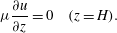
Consider a viscous fluid of dynamic viscosity
 ${\it\mu}$
and density
${\it\mu}$
and density
 ${\it\rho}$
, spreading horizontally under its own weight while another viscous fluid of dynamic viscosity
${\it\rho}$
, spreading horizontally under its own weight while another viscous fluid of dynamic viscosity
 ${\it\mu}_{l}$
and greater density
${\it\mu}_{l}$
and greater density
 ${\it\rho}_{l}$
intrudes beneath it as shown in figure 1. Although what follows applies for viscous fluids with general viscosity ratios, for the time being we will consider the underlying fluid to be less viscous, lubricating the overlying highly viscous current. There are two regions: a lubricated region involving both fluids; and a no-slip region involving the more viscous fluid only. The intruding current, of depth
${\it\rho}_{l}$
intrudes beneath it as shown in figure 1. Although what follows applies for viscous fluids with general viscosity ratios, for the time being we will consider the underlying fluid to be less viscous, lubricating the overlying highly viscous current. There are two regions: a lubricated region involving both fluids; and a no-slip region involving the more viscous fluid only. The intruding current, of depth
 $h(x,t)$
, extends to the lubrication, or intrusion, front
$h(x,t)$
, extends to the lubrication, or intrusion, front
 $x=x_{L}(t)$
. The upper fluid, with surface height
$x=x_{L}(t)$
. The upper fluid, with surface height
 $z=H(x,t)$
, extends to
$z=H(x,t)$
, extends to
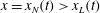 $x=x_{N}(t)>x_{L}(t)$
.
$x=x_{N}(t)>x_{L}(t)$
.
Beyond the intrusion front
 $x=x_{L}$
, the more viscous fluid propagates over a rigid horizontal surface and spreads analogously to a classical viscous gravity current (Huppert Reference Huppert1982), where stresses due to vertical shear provide the dominant resistance to flow. The lubricated region is more involved. Vertical shear stresses arising from traction along the rigid horizontal base dominate the dynamics of the underlying fluid. However, shear and extensional stress can both play a role within the overlying current. Extensional stress dominates if the lubricating layer exerts negligible shear stress on the overlying layer, in which case the flow in the upper layer is uniform to leading order. A further discussion is provided in § 6. We consider the alternative limit in which extensional stresses are negligible compared with either the viscous shear stress in the upper layer or to the stress exerted by the lower layer.
$x=x_{L}$
, the more viscous fluid propagates over a rigid horizontal surface and spreads analogously to a classical viscous gravity current (Huppert Reference Huppert1982), where stresses due to vertical shear provide the dominant resistance to flow. The lubricated region is more involved. Vertical shear stresses arising from traction along the rigid horizontal base dominate the dynamics of the underlying fluid. However, shear and extensional stress can both play a role within the overlying current. Extensional stress dominates if the lubricating layer exerts negligible shear stress on the overlying layer, in which case the flow in the upper layer is uniform to leading order. A further discussion is provided in § 6. We consider the alternative limit in which extensional stresses are negligible compared with either the viscous shear stress in the upper layer or to the stress exerted by the lower layer.
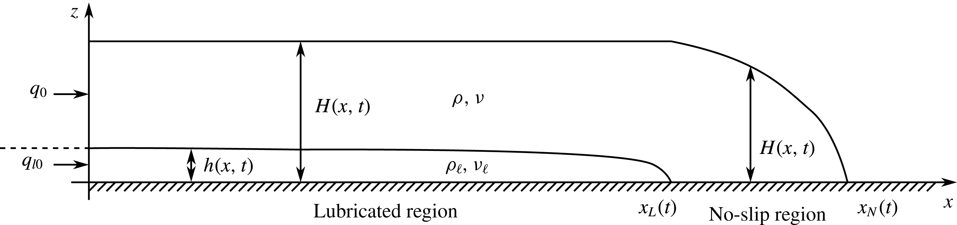
Figure 1. Schematic diagram illustrating the side profile of the flow of two superposed thin films of viscous fluid spreading under gravity on a rigid horizontal surface.
In developing a theoretical framework, we take into account viscous and buoyancy forces only and assume that inertial effects are negligible. We also neglect the effects of mixing and surface tension at the interface between the layers. We assume that the lengths of both currents are much greater than their thicknesses in both the lubricated and no-slip regions,
 $$\begin{eqnarray}h\ll x_{L}\quad \text{and}\quad H\ll \min (x_{L},x_{N}-x_{L}),\end{eqnarray}$$
and apply the approximations of lubrication theory.
2.1. No-slip region
The flow in the no-slip region forms a shear-dominated viscous gravity current with depth-integrated volume flux (Huppert Reference Huppert1982)
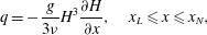 $$\begin{eqnarray}q=-\frac{g}{3{\it\nu}}H^{3}\frac{\partial H}{\partial x},\quad x_{L}\leqslant x\leqslant x_{N},\end{eqnarray}$$
which, together with a depth-integrated continuity equation, leads to the nonlinear diffusion equation
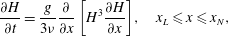 $$\begin{eqnarray}\frac{\partial H}{\partial t}=\frac{g}{3{\it\nu}}\frac{\partial }{\partial x}\left[H^{3}\frac{\partial H}{\partial x}\right]\!,\quad x_{L}\leqslant x\leqslant x_{N},\end{eqnarray}$$
satisfying
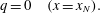 $$\begin{eqnarray}q=0\quad (x=x_{N}).\end{eqnarray}$$
Its rate of propagation is controlled by the global conservation equation
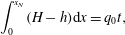 $$\begin{eqnarray}\int _{0}^{x_{N}}(H-h)\text{d}x=q_{0}t,\end{eqnarray}$$
or, equivalently, is controlled kinematically by the condition
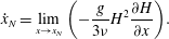 $$\begin{eqnarray}{\dot{x}}_{N}=\lim _{x\rightarrow x_{N}}\left(-\frac{g}{3{\it\nu}}H^{2}\frac{\partial H}{\partial x}\right)\!.\end{eqnarray}$$
2.2. Lubricated region
We restrict attention to the case in which both fluids in the lubricated region are resisted dominantly by viscous shear stresses. With the lubrication approximation, the pressures in the two films are given hydrostatically by
 $$\begin{eqnarray}\displaystyle & \displaystyle p=p_{0}+{\it\rho}g(H-z)\quad \text{for }h\leqslant z\leqslant H, & \displaystyle\end{eqnarray}$$
 $$\begin{eqnarray}\displaystyle & \displaystyle p_{l}=p_{0}+{\it\rho}g(H-h)+{\it\rho}_{l}g(h-z)\quad \text{for }0\leqslant z\leqslant h, & \displaystyle\end{eqnarray}$$
 $p_{0}$
is a constant ambient pressure. The governing equations for the fluid velocities are
$p_{0}$
is a constant ambient pressure. The governing equations for the fluid velocities are  $$\begin{eqnarray}{\it\mu}\frac{\partial ^{2}u}{\partial z^{2}}=\frac{\partial p}{\partial x}\quad \text{for }h\leqslant z\leqslant H,\quad {\it\mu}_{l}\frac{\partial ^{2}u_{l}}{\partial z^{2}}=\frac{\partial p_{l}}{\partial x}\quad \text{for }0\leqslant z\leqslant h,\end{eqnarray}$$
subject to
 $$\begin{eqnarray}u_{l}=0\quad (z=0),\end{eqnarray}$$
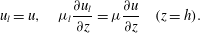 $$\begin{eqnarray}u_{l}=u,\quad {\it\mu}_{l}\frac{\partial u_{l}}{\partial z}={\it\mu}\frac{\partial u}{\partial z}\quad (z=h).\end{eqnarray}$$
 $$\begin{eqnarray}{\it\mu}\frac{\partial u}{\partial z}=0\quad (z=H).\end{eqnarray}$$
These boundary conditions represent no-slip at the base, continuity of velocity and shear stress between the layers, and no stress at the upper free surface. The solutions for the velocities of the two fluids in the lubricated region are
 $$\begin{eqnarray}\displaystyle u_{l}=-\frac{{\it\rho}g}{2{\it\mu}_{l}}\left[z(2h-z)\left(\mathscr{D}\frac{\partial h}{\partial x}+\frac{\partial H}{\partial x}\right)+2z(H-h)\frac{\partial H}{\partial x}\right]\!,\quad 0\leqslant z\leqslant h,\end{eqnarray}$$
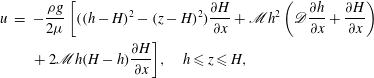 $$\begin{eqnarray}\displaystyle u & = & \displaystyle -\frac{{\it\rho}g}{2{\it\mu}}\left[((h-H)^{2}-(z-H)^{2})\frac{\partial H}{\partial x}+\mathscr{M}h^{2}\left(\mathscr{D}\frac{\partial h}{\partial x}+\frac{\partial H}{\partial x}\right)\right.\nonumber\\ \displaystyle & & \displaystyle \left.+\,2\mathscr{M}h(H-h)\frac{\partial H}{\partial x}\right]\!,\quad h\leqslant z\leqslant H,\end{eqnarray}$$
where
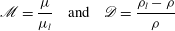 $$\begin{eqnarray}\mathscr{M}=\frac{{\it\mu}}{{\it\mu}_{l}}\quad \text{and}\quad \mathscr{D}=\frac{{\it\rho}_{l}-{\it\rho}}{{\it\rho}}\end{eqnarray}$$
are dimensionless parameters characterizing the dynamic viscosity ratio and density difference between the upper and lower layers. Integrating (2.13) vertically, we determine the volume flux of fluid, per unit width, in the lower film to be
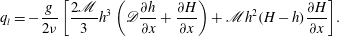 $$\begin{eqnarray}q_{l}=-\frac{g}{2{\it\nu}}\left[\frac{2\mathscr{M}}{3}h^{3}\left(\mathscr{D}\frac{\partial h}{\partial x}+\frac{\partial H}{\partial x}\right)+\mathscr{M}h^{2}(H-h)\frac{\partial H}{\partial x}\right]\!.\end{eqnarray}$$
The first group of terms on the right-hand side reflects a Poiseuille-like contribution to the flow of the lower layer resulting from the spreading of the film under its own weight and the weight of the fluid above it. The pressure gradient in the lower film depends on both surface heights if there is a density difference between the films. The second term is a Couette-like contribution induced by motion of the upper layer. Similarly, we determine the volume flux, per unit width, in the upper film to be
 $$\begin{eqnarray}\displaystyle q=-\frac{g}{2{\it\nu}}\left[\frac{2}{3}(H-h)^{3}\frac{\partial H}{\partial x}+\mathscr{M}\left(\mathscr{D}\frac{\partial h}{\partial x}+\frac{\partial H}{\partial x}\right)h^{2}(H-h)+2\mathscr{M}h(H-h)^{2}\frac{\partial H}{\partial x}\right]\!. & & \displaystyle \nonumber\\ \displaystyle & & \displaystyle\end{eqnarray}$$
The first term on the right-hand side reflects Poiseuille-like flow driven by gradients in the surface height. The second and third terms on the right-hand side, with prefactors proportional to
 $\mathscr{M}$
, are both Couette terms arising from boundary motion, resulting in uniform plug flow. With large values of
$\mathscr{M}$
, are both Couette terms arising from boundary motion, resulting in uniform plug flow. With large values of
 $\mathscr{M}$
, these terms can dominate the flow as discussed in later parts of this paper. This is important in the geophysical context as it indicates that subglacial lubrication can result in a flow that is appreciably plug-like within lubricated ice sheets.
$\mathscr{M}$
, these terms can dominate the flow as discussed in later parts of this paper. This is important in the geophysical context as it indicates that subglacial lubrication can result in a flow that is appreciably plug-like within lubricated ice sheets.
There is an interfacial velocity
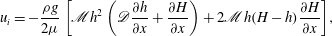 $$\begin{eqnarray}u_{i}=-\frac{{\it\rho}g}{2{\it\mu}}\left[\mathscr{M}h^{2}\left(\mathscr{D}\frac{\partial h}{\partial x}+\frac{\partial H}{\partial x}\right)+2\mathscr{M}h(H-h)\frac{\partial H}{\partial x}\right]\!,\end{eqnarray}$$
arising from boundary motion and interfacial shear stress
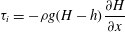 $$\begin{eqnarray}{\it\tau}_{i}=-{\it\rho}g(H-h)\frac{\partial H}{\partial x}\end{eqnarray}$$
arising from the spreading of the upper film under its weight. For
 $h\ll H$
, the interfacial shear stress and velocity are related linearly by
$h\ll H$
, the interfacial shear stress and velocity are related linearly by
 $$\begin{eqnarray}u_{i}\approx \frac{h}{{\it\mu}_{l}}{\it\tau}_{i}.\end{eqnarray}$$
This is a sliding law in which the sliding coefficient depends on the lower film thickness. It has a similar structure to the sliding law
 ${\it\tau}=Cu^{1/n}$
used in many glaciological studies (Weertman Reference Weertman1957, Reference Weertman1964; Nye Reference Nye1969; Kamb Reference Kamb1970; Fowler Reference Fowler1981) with
${\it\tau}=Cu^{1/n}$
used in many glaciological studies (Weertman Reference Weertman1957, Reference Weertman1964; Nye Reference Nye1969; Kamb Reference Kamb1970; Fowler Reference Fowler1981) with
 $n=1$
reflecting Newtonian rheology.
$n=1$
reflecting Newtonian rheology.
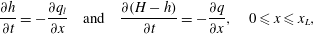
Conservation of mass in the two layers is described by
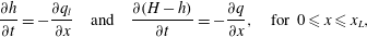 $$\begin{eqnarray}\frac{\partial h}{\partial t}=-\frac{\partial q_{l}}{\partial x}\quad \text{and}\quad \frac{\partial (H-h)}{\partial t}=-\frac{\partial q}{\partial x},\quad \text{for }0\leqslant x\leqslant x_{L},\end{eqnarray}$$
which are subject to
 $$\begin{eqnarray}q=q_{0},\quad q_{l}=q_{l0}\quad (x=0),\end{eqnarray}$$
 $$\begin{eqnarray}q_{l}=0,\quad q^{-}=q^{+}\quad (x=x_{L}).\end{eqnarray}$$
Flux continuity follows from continuity of height and local mass conservation. The free boundary
 $x=x_{L}$
is determined by
$x=x_{L}$
is determined by
 $$\begin{eqnarray}\int _{0}^{x_{L}}h\,\text{d}x=q_{l0}t\end{eqnarray}$$
or, equivalently, by
 $$\begin{eqnarray}{\dot{x}}_{L}=\lim _{x\rightarrow x_{L}}q_{l}/h.\end{eqnarray}$$
2.3. Initial transient after intrusion
We consider a general case in which there is a specified time difference
 $\mathscr{T}$
between the initiation of the flows of the two fluids. We found it practical that
$\mathscr{T}$
between the initiation of the flows of the two fluids. We found it practical that
 $\mathscr{T}\neq 0$
in laboratory experiments (see later), especially if the underlying fluid is of much lower viscosity than that of the overlying fluid. For times
$\mathscr{T}\neq 0$
in laboratory experiments (see later), especially if the underlying fluid is of much lower viscosity than that of the overlying fluid. For times
 $t<\mathscr{T}$
, we assume that the more viscous fluid spreads as a classical no-slip current and use the associated similarity solution (Huppert Reference Huppert1982) as an initial condition at
$t<\mathscr{T}$
, we assume that the more viscous fluid spreads as a classical no-slip current and use the associated similarity solution (Huppert Reference Huppert1982) as an initial condition at
 $t=\mathscr{T}$
for a numerical solution of our new mathematical model.
$t=\mathscr{T}$
for a numerical solution of our new mathematical model.
We first non-dimensionalize by writing
 $$\begin{eqnarray}(H,h)\equiv \mathscr{H}(\widehat{H},\widehat{h})\equiv (q_{0}^{2}{\it\nu}g^{-1}\mathscr{T})^{1/5}(\widehat{H},\widehat{h}),\quad x\equiv \mathscr{X}\widehat{x}\equiv (gq_{0}^{3}{\it\nu}^{-1}\mathscr{T}^{4})^{1/5}\widehat{x},\quad t\equiv \mathscr{T}\,\widehat{t}.\end{eqnarray}$$
The length scales
 $\mathscr{H}$
and
$\mathscr{H}$
and
 $\mathscr{X}$
characterize the thickness and extent of the classical single-fluid current at time
$\mathscr{X}$
characterize the thickness and extent of the classical single-fluid current at time
 $\mathscr{T}$
. Here,
$\mathscr{T}$
. Here,
 $\widehat{t}=1$
corresponds to the time of intrusion and the equations below apply for
$\widehat{t}=1$
corresponds to the time of intrusion and the equations below apply for
 $\widehat{t}\geqslant 1$
. After substitution and dropping hats, our model can be summarized as
$\widehat{t}\geqslant 1$
. After substitution and dropping hats, our model can be summarized as
 $$\begin{eqnarray}\displaystyle & \displaystyle q_{l}=-\frac{\mathscr{M}}{3}h^{3}\left(\mathscr{D}\frac{\partial h}{\partial x}+\frac{\partial H}{\partial x}\right)-\frac{\mathscr{M}}{2}h^{2}(H-h)\frac{\partial H}{\partial x},\quad 0\leqslant x\leqslant x_{L} & \displaystyle\end{eqnarray}$$
 $$\begin{eqnarray}\displaystyle & \displaystyle q=-\frac{1}{3}(H-h)^{3}\frac{\partial H}{\partial x}-\frac{\mathscr{M}}{2}h^{2}(H-h)\left(\mathscr{D}\frac{\partial h}{\partial x}+\frac{\partial H}{\partial x}\right)-\mathscr{M}h(H-h)^{2}\frac{\partial H}{\partial x},\quad 0\leqslant x\leqslant x_{L} & \displaystyle \nonumber\\ \displaystyle & & \displaystyle\end{eqnarray}$$
 $$\begin{eqnarray}\displaystyle & \displaystyle q=-\frac{1}{3}H^{3}\frac{\partial H}{\partial x},\quad x_{L}\leqslant x\leqslant x_{N} & \displaystyle\end{eqnarray}$$
 $$\begin{eqnarray}\frac{\partial h}{\partial t}=-\frac{\partial q_{l}}{\partial x}\quad \text{and}\quad \frac{\partial (H-h)}{\partial t}=-\frac{\partial q}{\partial x},\quad 0\leqslant x\leqslant x_{L},\end{eqnarray}$$
 $$\begin{eqnarray}\frac{\partial H}{\partial t}=-\frac{\partial q}{\partial x},\quad x_{L}\leqslant x\leqslant x_{N},\end{eqnarray}$$
 $$\begin{eqnarray}q_{l}=\mathscr{Q},\quad q=1\quad (x=0),\end{eqnarray}$$
 $$\begin{eqnarray}H^{-}=H^{+},\quad q^{-}=q^{+}\quad (x=x_{L}),\end{eqnarray}$$
 $$\begin{eqnarray}q_{l}=0\quad (x=x_{L}),\quad q=0\quad (x=x_{N}),\end{eqnarray}$$
 $$\begin{eqnarray}{\dot{x}}_{L}=\lim _{x\rightarrow x_{L}}q_{l}/h,\quad {\dot{x}}_{N}=\lim _{x\rightarrow x_{N}}q/H.\end{eqnarray}$$
The condition (2.33a,b
) is explained in § 2.4.1. Here, the dimensionless constant
 $\mathscr{Q}=q_{l0}/q_{0}$
is the ratio of the lower to upper fluid source fluxes. Three dimensionless parameters appear in the model equations, namely the dynamic viscosity ratio
$\mathscr{Q}=q_{l0}/q_{0}$
is the ratio of the lower to upper fluid source fluxes. Three dimensionless parameters appear in the model equations, namely the dynamic viscosity ratio
 $\mathscr{M}$
, density difference
$\mathscr{M}$
, density difference
 $\mathscr{D}$
and source flux ratio
$\mathscr{D}$
and source flux ratio
 $\mathscr{Q}$
.
$\mathscr{Q}$
.
The governing equations are a system in which both the lubricated and no-slip regions have moving boundaries. The equations were solved numerically using a second-order, finite-difference scheme after mapping the lubricated and no-slip regions to two fixed non-uniform grids on the interval
 $[0,1]$
, with grid points concentrated near the fronts. There are additional difficulties associated with the fact that the solutions at the fronts of the currents are singular. To remedy this, the transformed domains for the lubricated and no-slip regions were divided into equal intervals
$[0,1]$
, with grid points concentrated near the fronts. There are additional difficulties associated with the fact that the solutions at the fronts of the currents are singular. To remedy this, the transformed domains for the lubricated and no-slip regions were divided into equal intervals
 $\{[{\it\zeta}_{i-1/2},{\it\zeta}_{i+1/2}]:i=1,\dots ,n\}$
and the derivatives were evaluated at the midpoints
$\{[{\it\zeta}_{i-1/2},{\it\zeta}_{i+1/2}]:i=1,\dots ,n\}$
and the derivatives were evaluated at the midpoints
 ${\it\zeta}_{i}$
of these intervals using central differences. We applied the kinematic conditions (2.35a,b
) at
${\it\zeta}_{i}$
of these intervals using central differences. We applied the kinematic conditions (2.35a,b
) at
 ${\it\zeta}_{n}$
, where the solutions are not singular. The conditions that
${\it\zeta}_{n}$
, where the solutions are not singular. The conditions that
 $h=0$
at
$h=0$
at
 $x=x_{L}$
and
$x=x_{L}$
and
 $H=0$
at
$H=0$
at
 $x=x_{N}$
, which are a consequence of (2.34a,b
) and (2.35a,b
), were applied at
$x=x_{N}$
, which are a consequence of (2.34a,b
) and (2.35a,b
), were applied at
 ${\it\zeta}_{n+1/2}$
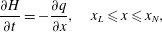
. A Matlab ODE solver was used for integration in time. An illustrative solution of the full system of partial differential equations (PDEs) (2.27)–(2.35) is presented in figure 2. The parameter values used,
${\it\zeta}_{n+1/2}$
. A Matlab ODE solver was used for integration in time. An illustrative solution of the full system of partial differential equations (PDEs) (2.27)–(2.35) is presented in figure 2. The parameter values used,
 $\mathscr{M}=10\,000$
,
$\mathscr{M}=10\,000$
,
 $\mathscr{D}=0.1$
, and
$\mathscr{D}=0.1$
, and
 $\mathscr{Q}=0.2$
, are typical of our experiments described in § 4.
$\mathscr{Q}=0.2$
, are typical of our experiments described in § 4.
Figure 2. Solutions of the full system of partial differential equations (PDEs) (2.27)–(2.35) for two-dimensional spreading with
 $\mathscr{M}=10\,000$
,
$\mathscr{M}=10\,000$
,
 $\mathscr{D}=0.1$
and
$\mathscr{D}=0.1$
and
 $\mathscr{Q}=0.2$
. (a) Profile thicknesses as functions of
$\mathscr{Q}=0.2$
. (a) Profile thicknesses as functions of
 $x$
at dimensionless times
$x$
at dimensionless times
 $t=1.1,2,3$
. Surface heights are solid curves and interfacial heights are dashed. (b) Frontal positions and (c) source thicknesses as functions of
$t=1.1,2,3$
. Surface heights are solid curves and interfacial heights are dashed. (b) Frontal positions and (c) source thicknesses as functions of
 $t$
for the upper (bold solid) and lower (bold dashed) films. The solutions of the PDEs (2.27)–(2.35) in (b,c) undergo an initial transient and converge to the self-similar solutions (2.38)–(2.47) marked by thin black horizontal lines as
$t$
for the upper (bold solid) and lower (bold dashed) films. The solutions of the PDEs (2.27)–(2.35) in (b,c) undergo an initial transient and converge to the self-similar solutions (2.38)–(2.47) marked by thin black horizontal lines as
 $t\rightarrow \infty$
. The
$t\rightarrow \infty$
. The
 $y$
-axes in (b,c) are scaled time-dependently with respect to the long-time similarity solution.
$y$
-axes in (b,c) are scaled time-dependently with respect to the long-time similarity solution.
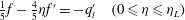
Representative profile thicknesses of both layers undergoing an initial transient after the intrusion of the low viscosity fluid are shown in figure 2(a) at various values of the dimensionless time
 $t$
. The upper surface noticeably flattens with the presence of the lubricant and its height initially decreases. The presence of the lubricant accelerates and thins the high-viscosity fluid. This can also be inferred from the other two subfigures. Figure 2(b) shows the frontal positions of both fluid films before and after introduction of the lubricant. The frontal position of the high-viscosity film undergoes an initial transient and advances more rapidly than it would have without the lubricant. Figure 2(c) shows the source thicknesses of both films before and after the intrusion of the lubricant. The upper film thins as a result of the intrusion. The frontal positions and source thicknesses of both films undergo an initial transient and converge towards a self-similar solution (thin curves in figure 2
b,c), which is the topic of the next section.
$t$
. The upper surface noticeably flattens with the presence of the lubricant and its height initially decreases. The presence of the lubricant accelerates and thins the high-viscosity fluid. This can also be inferred from the other two subfigures. Figure 2(b) shows the frontal positions of both fluid films before and after introduction of the lubricant. The frontal position of the high-viscosity film undergoes an initial transient and advances more rapidly than it would have without the lubricant. Figure 2(c) shows the source thicknesses of both films before and after the intrusion of the lubricant. The upper film thins as a result of the intrusion. The frontal positions and source thicknesses of both films undergo an initial transient and converge towards a self-similar solution (thin curves in figure 2
b,c), which is the topic of the next section.
2.4. Self-similar solution
At large times
 $t\gg \mathscr{T}$
, there is a lack of dimensional information to determine an intrinsic length scale and one can anticipate the system tending towards self-similarity. Motivated by this, we reformulate the problem in terms of the similarity variable
$t\gg \mathscr{T}$
, there is a lack of dimensional information to determine an intrinsic length scale and one can anticipate the system tending towards self-similarity. Motivated by this, we reformulate the problem in terms of the similarity variable
 $$\begin{eqnarray}{\it\eta}=x/(gq_{0}^{3}{\it\nu}^{-1}t^{4})^{1/5}\end{eqnarray}$$
and write the solutions in the form
 $$\begin{eqnarray}[H(x,t),h(x,t)]=(q_{0}^{2}{\it\nu}g^{-1}t)^{1/5}[F({\it\eta}),f({\it\eta})],\end{eqnarray}$$
using the same scaling as for an unlubricated gravity current.
Substitution of the self-similar forms of solutions (2.36)–(2.37) into the governing equations leads to the coupled system of ordinary differential equations (ODEs)
 $$\begin{eqnarray}\displaystyle & \displaystyle q_{l}=-\frac{\mathscr{M}}{3}f^{3}[\mathscr{D}f^{\prime }+F^{\prime }]-\frac{\mathscr{M}}{2}f^{2}(F-f)F^{\prime }\quad (0\leqslant {\it\eta}\leqslant {\it\eta}_{L}) & \displaystyle\end{eqnarray}$$
 $$\begin{eqnarray}\displaystyle & \displaystyle q=-\displaystyle \frac{1}{3}(F-f)^{3}F^{\prime }-\frac{\mathscr{M}}{2}f^{2}(F-f)[\mathscr{D}f^{\prime }+F^{\prime }]-\mathscr{M}f(F-f)^{2}F^{\prime }\quad (0\leqslant {\it\eta}\leqslant {\it\eta}_{L}) & \displaystyle\end{eqnarray}$$
 $$\begin{eqnarray}\displaystyle & q=-{\textstyle \frac{1}{3}}F^{3}F^{\prime }\quad ({\it\eta}_{L}\leqslant {\it\eta}\leqslant {\it\eta}_{N}) & \displaystyle\end{eqnarray}$$
 $$\begin{eqnarray}\displaystyle & {\textstyle \frac{1}{5}}f-{\textstyle \frac{4}{5}}{\it\eta}f^{\prime }=-q_{l}^{\prime }\quad (0\leqslant {\it\eta}\leqslant {\it\eta}_{L}) & \displaystyle\end{eqnarray}$$
 $$\begin{eqnarray}\displaystyle & {\textstyle \frac{1}{5}}(F-f)-{\textstyle \frac{4}{5}}{\it\eta}(F^{\prime }-f^{\prime })=-q^{\prime }\quad (0\leqslant {\it\eta}\leqslant {\it\eta}_{L}) & \displaystyle\end{eqnarray}$$
 $$\begin{eqnarray}\displaystyle & {\textstyle \frac{1}{5}}F-{\textstyle \frac{4}{5}}{\it\eta}F^{\prime }=-q^{\prime }\quad ({\it\eta}_{L}\leqslant {\it\eta}\leqslant {\it\eta}_{N}) & \displaystyle\end{eqnarray}$$
 $$\begin{eqnarray}q_{l}=\mathscr{Q},\quad q=1\quad ({\it\eta}=0)\end{eqnarray}$$
 $$\begin{eqnarray}F^{-}=F^{+},\quad q^{-}=q^{+}\quad ({\it\eta}={\it\eta}_{L})\end{eqnarray}$$
 $$\begin{eqnarray}f=0\quad ({\it\eta}={\it\eta}_{L}),\quad F=0\quad ({\it\eta}={\it\eta}_{N})\end{eqnarray}$$
 $$\begin{eqnarray}{\textstyle \frac{4}{5}}{\it\eta}_{L}=\lim _{{\it\eta}\rightarrow {\it\eta}_{L}}q_{l}/f,\quad {\textstyle \frac{4}{5}}{\it\eta}_{N}=\lim _{{\it\eta}\rightarrow {\it\eta}_{N}}q/F.\end{eqnarray}$$
Here, we denote by
 ${\it\eta}_{L}$
and
${\it\eta}_{L}$
and
 ${\it\eta}_{N}$
the values of
${\it\eta}_{N}$
the values of
 ${\it\eta}$
corresponding to the endpoints
${\it\eta}$
corresponding to the endpoints
 $x=x_{L}$
and
$x=x_{L}$
and
 $x=x_{N}$
, respectively.
$x=x_{N}$
, respectively.
This model encompasses a general class of two-layer gravity currents, which we explore in § 5, ranging from extremes such as thin lubricating layers underneath a more viscous fluid to the inverse situation of a thin surface film coating an underlying current.
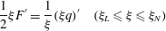
2.4.1. Asymptotic behaviour near the fronts
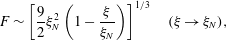
The thickness of the current near the front of the unlubricated region obeys
 $$\begin{eqnarray}F\sim \left[\frac{36}{5}{\it\eta}_{N}^{2}\left(1-\frac{{\it\eta}}{{\it\eta}_{N}}\right)\right]^{1/3}\quad \text{as }{\it\eta}\rightarrow {\it\eta}_{N}\end{eqnarray}$$
as found previously for a single-fluid current (Huppert Reference Huppert1982).
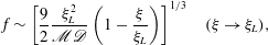
Provided the density difference is non-zero, we find a consistent asymptotic approximation in which the surface slope is finite while the thickness of the lubricating layer is singular at the lubrication front, given by
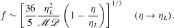 $$\begin{eqnarray}f\sim \left[\frac{36}{5}\frac{{\it\eta}_{L}^{2}}{\mathscr{M}\mathscr{D}}\left(1-\frac{{\it\eta}}{{\it\eta}_{L}}\right)\right]^{1/3}\quad ({\it\eta}\rightarrow {\it\eta}_{L}).\end{eqnarray}$$
This singular behaviour implies that the lubricating fluid spreads under the action of its own weight near its leading front. The viscosity ratio
 $\mathscr{M}$
appears because of our choice in scaling the similarity variables with respect to the upper fluid and the prefactor
$\mathscr{M}$
appears because of our choice in scaling the similarity variables with respect to the upper fluid and the prefactor
 $\mathscr{D}$
essentially derives from the fact that a viscous fluid intruding underneath a layer of less dense viscous fluid of much greater thickness spreads under the action of a reduced gravity
$\mathscr{D}$
essentially derives from the fact that a viscous fluid intruding underneath a layer of less dense viscous fluid of much greater thickness spreads under the action of a reduced gravity
 $g^{\prime }=\mathscr{D}g$
.
$g^{\prime }=\mathscr{D}g$
.
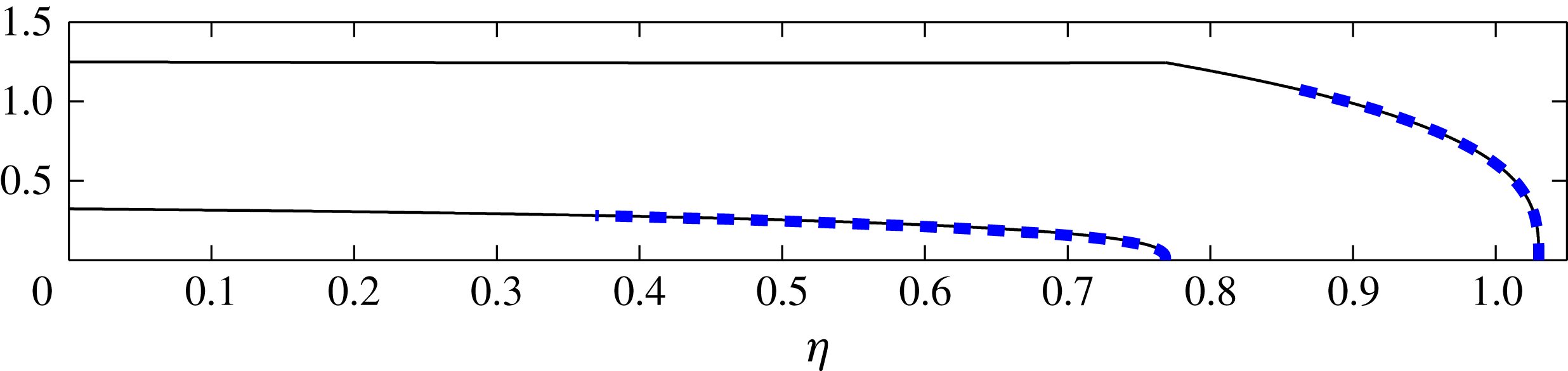
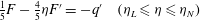
Figure 3. Similarity solutions and asymptotic results in two dimensions. Solutions of (2.38)–(2.47) for the thicknesses of both currents are presented as solid curves. Asymptotic solutions (2.48) and (2.49) near the two fronts are presented as dashed bold curves. Parameter values used are
 $\mathscr{M}=100$
,
$\mathscr{M}=100$
,
 $\mathscr{D}=1$
and
$\mathscr{D}=1$
and
 $\mathscr{Q}=0.2$
.
$\mathscr{Q}=0.2$
.
Continuity of flux (2.45a,b ) expressed in terms of layer thicknesses using (2.39) and (2.40) determines the discontinuity in surface slope
 $$\begin{eqnarray}[F^{\prime }]_{-}^{+}=-\frac{18}{5}\frac{{\it\eta}_{L}}{F^{2}}\quad ({\it\eta}={\it\eta}_{L}).\end{eqnarray}$$
The minus sign indicates that the upstream surface slope is smaller in magnitude than the downstream slope, allowing for gentler slopes, flatness or even a reversal in slope upstream of the lubricating front. This change in slope is consistent with the intuition that the presence of a lubricating layer of fluid tends to thin the more viscous fluid above it. The result above uses the condition (2.33a
) of thickness continuity at the lubrication front, which can be derived by integrating (2.30) in the vicinity of the lubrication front, using flux continuity and the fact that
 ${\dot{x}}_{L}\neq 0$
.
${\dot{x}}_{L}\neq 0$
.
The asymptotic solutions above were used as starting conditions in solving the ODEs (2.38)–(2.47) numerically using a shooting method, with
 ${\it\eta}_{L}$
and
${\it\eta}_{L}$
and
 ${\it\eta}_{N}$
as shooting parameters. The equations were integrated inwards with a Matlab ODE solver from
${\it\eta}_{N}$
as shooting parameters. The equations were integrated inwards with a Matlab ODE solver from
 ${\it\eta}={\it\eta}_{N}$
using (2.48) and matched at
${\it\eta}={\it\eta}_{N}$
using (2.48) and matched at
 ${\it\eta}={\it\eta}_{L}$
using (2.49) and (2.50). An illustrative solution of (2.38)–(2.47) is presented in figure 3 along with the asymptotic solutions (2.48) and (2.49). The solution of the full PDEs (2.27)–(2.35) is shown to converge to the similarity solution as
${\it\eta}={\it\eta}_{L}$
using (2.49) and (2.50). An illustrative solution of (2.38)–(2.47) is presented in figure 3 along with the asymptotic solutions (2.48) and (2.49). The solution of the full PDEs (2.27)–(2.35) is shown to converge to the similarity solution as
 $t\rightarrow \infty$
in figure 2. The dependences of
$t\rightarrow \infty$
in figure 2. The dependences of
 ${\it\eta}_{N}$
and
${\it\eta}_{N}$
and
 ${\it\eta}_{L}$
on
${\it\eta}_{L}$
on
 $\mathscr{Q},\mathscr{D}$
and
$\mathscr{Q},\mathscr{D}$
and
 $\mathscr{M}$
are shown graphically in § 5.
$\mathscr{M}$
are shown graphically in § 5.
3. Axisymmetric lubricated currents
The theoretical development for axisymmetric spreading is similar to the two-dimensional case. For brevity, we show only the major equations that are affected by the changed geometry.
3.1. No-slip region
The flow in the no-slip region behaves as a classical viscous gravity current governed by
 $$\begin{eqnarray}\frac{\partial H}{\partial t}=\frac{g}{3{\it\nu}}\frac{1}{r}\frac{\partial }{\partial r}\left(rH^{3}\frac{\partial H}{\partial r}\right)\end{eqnarray}$$
subject to the global continuity equation
 $$\begin{eqnarray}2{\rm\pi}\int _{0}^{r_{N}}(H-h)r\,\text{d}r=Q_{0}t,\end{eqnarray}$$
where
 $Q_{0}$
is a prescribed radial input flux of the high-viscosity fluid and
$Q_{0}$
is a prescribed radial input flux of the high-viscosity fluid and
 $h$
is defined to vanish outside the disc of radius
$h$
is defined to vanish outside the disc of radius
 $r_{L}$
.
$r_{L}$
.
3.2. Lubricated region
Following the analysis of the two-dimensional case, conservation of mass within a radial slice of both films gives
 $$\begin{eqnarray}\frac{\partial h}{\partial t}=-\frac{1}{r}\frac{\partial }{\partial r}(rq_{l})\quad \text{and}\quad \frac{\partial (H-h)}{\partial t}=-\frac{1}{r}\frac{\partial }{\partial r}(rq),\quad \text{for }0\leqslant r\leqslant r_{L},\end{eqnarray}$$
where
 $q_{l}$
and
$q_{l}$
and
 $q$
are as given in (2.16) and (2.17) with the variable
$q$
are as given in (2.16) and (2.17) with the variable
 $x$
replaced by
$x$
replaced by
 $r$
. We denote by
$r$
. We denote by
 $Q$
and
$Q$
and
 $Q_{l}$
the radial flux out of a circular region of radius
$Q_{l}$
the radial flux out of a circular region of radius
 $r$
, of the upper and lower layers. Explicitly,
$r$
, of the upper and lower layers. Explicitly,
 $$\begin{eqnarray}Q=2{\rm\pi}rq\quad \text{and}\quad Q_{l}=2{\rm\pi}rq_{l}.\end{eqnarray}$$
The evolution of
 $r=r_{L}$
is determined from the global continuity equation,
$r=r_{L}$
is determined from the global continuity equation,
 $$\begin{eqnarray}2{\rm\pi}\int _{0}^{r_{L}}hr\text{d}r=Q_{l0}t,\end{eqnarray}$$
where
 $Q_{l0}$
is a prescribed radial input flux of lubricant. The input flux conditions are given by
$Q_{l0}$
is a prescribed radial input flux of lubricant. The input flux conditions are given by
 $$\begin{eqnarray}Q=Q_{0}\quad \text{and}\quad Q_{l}=Q_{l0}\quad \text{at }r=0.\end{eqnarray}$$
The remaining boundary conditions are analogous to the two-dimensional case.
3.3. Initial transient after intrusion
With a time-delay
 $\mathscr{T}$
between the initiation of flow in the two layers, an initial transient develops and precludes self-similarity. A similar situation has been introduced in § 2.3, however there are differences in the governing equations due to the change in geometry. We non-dimensionalize by
$\mathscr{T}$
between the initiation of flow in the two layers, an initial transient develops and precludes self-similarity. A similar situation has been introduced in § 2.3, however there are differences in the governing equations due to the change in geometry. We non-dimensionalize by
 $$\begin{eqnarray}\displaystyle (H,h)\equiv \mathscr{H}(\widehat{H},\widehat{h})\equiv ({\it\nu}q_{0}g^{-1})^{1/4}(\widehat{H},\widehat{h}),\quad r\equiv \mathscr{R}\widehat{r}\equiv (gq_{0}^{3}{\it\nu}^{-1}\mathscr{T}^{4})^{1/8}\widehat{r},\quad t\equiv \mathscr{T}\widehat{t} & & \displaystyle \nonumber\\ \displaystyle & & \displaystyle\end{eqnarray}$$
where
 $\mathscr{H}$
and
$\mathscr{H}$
and
 $\mathscr{R}$
characterize the thickness and frontal position of a classical single-fluid current at time
$\mathscr{R}$
characterize the thickness and frontal position of a classical single-fluid current at time
 $\mathscr{T}$
. Here,
$\mathscr{T}$
. Here,
 $\widehat{t}=1$
corresponds to the time of intrusion and the equations below apply for
$\widehat{t}=1$
corresponds to the time of intrusion and the equations below apply for
 $\widehat{t}\geqslant 1$
. This gives, dropping hats,
$\widehat{t}\geqslant 1$
. This gives, dropping hats,
 $$\begin{eqnarray}\displaystyle & \displaystyle q_{l}=-\frac{\mathscr{M}}{3}h^{3}\left(\mathscr{D}\frac{\partial h}{\partial r}+\frac{\partial H}{\partial r}\right)-\frac{\mathscr{M}}{2}h^{2}(H-h)\frac{\partial H}{\partial r},\quad 0\leqslant r\leqslant r_{L} & \displaystyle\end{eqnarray}$$
 $$\begin{eqnarray}\displaystyle & \displaystyle q=-\frac{1}{3}(H-h)^{3}\frac{\partial H}{\partial r}-\frac{\mathscr{M}}{2}h^{2}(H-h)\left(\mathscr{D}\frac{\partial h}{\partial r}+\frac{\partial H}{\partial r}\right)-\mathscr{M}h(H-h)^{2}\frac{\partial H}{\partial r},\quad 0\leqslant r\leqslant r_{L} & \displaystyle \nonumber\\ \displaystyle & & \displaystyle\end{eqnarray}$$
 $$\begin{eqnarray}\displaystyle & \displaystyle q=-\frac{1}{3}H^{3}\frac{\partial H}{\partial r},\quad r_{L}\leqslant r\leqslant r_{N} & \displaystyle\end{eqnarray}$$
 $$\begin{eqnarray}\frac{\partial h}{\partial t}=-\frac{1}{r}\frac{\partial }{\partial r}(rq_{l})\quad \text{and}\quad \frac{\partial (H-h)}{\partial t}=-\frac{1}{r}\frac{\partial }{\partial r}(rq),\quad 0\leqslant r\leqslant r_{L},\end{eqnarray}$$
 $$\begin{eqnarray}\frac{\partial H}{\partial t}=-\frac{1}{r}\frac{\partial }{\partial r}(rq),\quad r_{L}\leqslant r\leqslant r_{N},\end{eqnarray}$$
 $$\begin{eqnarray}\lim _{r\rightarrow 0}(2{\rm\pi}rq_{l})=\mathscr{Q}\quad \text{and}\quad \lim _{r\rightarrow 0}(2{\rm\pi}rq)=1,\end{eqnarray}$$
 $$\begin{eqnarray}H^{-}=H^{+}\quad \text{and}\quad q^{-}=q^{+}\quad \text{at }r=r_{L},\end{eqnarray}$$
 $$\begin{eqnarray}q_{l}=0\quad \text{at}\quad r=r_{L}\quad \text{and}\quad q=0\quad \text{at }r=r_{N},\end{eqnarray}$$
 $$\begin{eqnarray}{\dot{r}}_{L}=\lim _{x\rightarrow x_{L}}q_{l}/h\quad \text{and}\quad {\dot{r}}_{N}=\lim _{x\rightarrow x_{N}}q/H.\end{eqnarray}$$
Here, the dimensionless constant
 $\mathscr{Q}=Q_{l0}/Q_{0}$
is the ratio of the lower to upper fluid source fluxes. The equations above depend on three dimensionless parameters: the viscosity ratio
$\mathscr{Q}=Q_{l0}/Q_{0}$
is the ratio of the lower to upper fluid source fluxes. The equations above depend on three dimensionless parameters: the viscosity ratio
 $\mathscr{M}$
; density difference
$\mathscr{M}$
; density difference
 $\mathscr{D}$
; and source flux ratio
$\mathscr{D}$
; and source flux ratio
 $\mathscr{Q}$
.
$\mathscr{Q}$
.
Figure 4. Solutions of the full system of PDEs (3.8)–(3.16) for axisymmetric spreading with
 $\mathscr{M}=10\,000$
,
$\mathscr{M}=10\,000$
,
 $\mathscr{D}=0.1$
and
$\mathscr{D}=0.1$
and
 $\mathscr{Q}=0.2$
. (a) Profile thicknesses as functions of
$\mathscr{Q}=0.2$
. (a) Profile thicknesses as functions of
 $x$
at dimensionless times
$x$
at dimensionless times
 $t=1.01,2,3$
. Surface heights are solid curves and interfacial heights are dashed. (b) Frontal positions as functions of
$t=1.01,2,3$
. Surface heights are solid curves and interfacial heights are dashed. (b) Frontal positions as functions of
 $t$
for the upper (bold solid) and lower (bold dashed) films. (c) Thickness of the upper film at
$t$
for the upper (bold solid) and lower (bold dashed) films. (c) Thickness of the upper film at
 $r=r_{L}$
(bold solid) as a function of
$r=r_{L}$
(bold solid) as a function of
 $t$
. The solutions of the PDEs (3.8)–(3.16) in (b,c) undergo an initial transient and converge to the self-similar solutions (3.19)–(3.28) marked by thin black horizontal lines as
$t$
. The solutions of the PDEs (3.8)–(3.16) in (b,c) undergo an initial transient and converge to the self-similar solutions (3.19)–(3.28) marked by thin black horizontal lines as
 $t\rightarrow \infty$
. The
$t\rightarrow \infty$
. The
 $y$
-axes in (b,c) are scaled time-dependently with respect to the long-time similarity solution.
$y$
-axes in (b,c) are scaled time-dependently with respect to the long-time similarity solution.
A typical solution of the full system of PDEs (3.8)–(3.16) is presented in figure 4 for parameter values (
 $\mathscr{M}=10\,000$
,
$\mathscr{M}=10\,000$
,
 $\mathscr{D}=0.1$
and
$\mathscr{D}=0.1$
and
 $\mathscr{Q}=0.2$
) that are close to our experiments. We used a numerical method similar to that of § 2.3, but with uniformly spaced grids. Figure 4(a) shows the thicknesses of the upper and lower layer against the radial coordinate undergoing an initial transient after intrusion at various dimensionless values of
$\mathscr{Q}=0.2$
) that are close to our experiments. We used a numerical method similar to that of § 2.3, but with uniformly spaced grids. Figure 4(a) shows the thicknesses of the upper and lower layer against the radial coordinate undergoing an initial transient after intrusion at various dimensionless values of
 $t$
. Figure 4(b) shows the frontal positions
$t$
. Figure 4(b) shows the frontal positions
 $r_{L}$
and
$r_{L}$
and
 $r_{N}$
before and after intrusion as functions of
$r_{N}$
before and after intrusion as functions of
 $t$
. There is a slight perturbation near
$t$
. There is a slight perturbation near
 $t=1$
of the curve for
$t=1$
of the curve for
 $r_{N}$
due to the choice of resolution and initialization of the computations. Figure 4(c) shows the upper surface height at
$r_{N}$
due to the choice of resolution and initialization of the computations. Figure 4(c) shows the upper surface height at
 $r_{L}$
, rather than at the source as there is a weak logarithmic singularity at the origin as a result of fluid being introduced from a single point. The singularity is less visible on the length scale of the currents for this choice of parameters. There is a similar behaviour at the origin in the extended two-dimensional problem, with two half spaces
$r_{L}$
, rather than at the source as there is a weak logarithmic singularity at the origin as a result of fluid being introduced from a single point. The singularity is less visible on the length scale of the currents for this choice of parameters. There is a similar behaviour at the origin in the extended two-dimensional problem, with two half spaces
 $(-\infty ,0]$
and
$(-\infty ,0]$
and
 $[0,\infty )$
, but this time in the form of a jump discontinuity in the surface slope. The qualitative effects of the lubricant in the axisymmetric setting are seen to be similar to those found in two dimensions.
$[0,\infty )$
, but this time in the form of a jump discontinuity in the surface slope. The qualitative effects of the lubricant in the axisymmetric setting are seen to be similar to those found in two dimensions.
3.4. Self-similarity
After the initial transient caused by a delay in initiation of flow in the lower film, the flow converges towards a similarity solution described in terms of the similarity variable
 $$\begin{eqnarray}{\it\xi}=r/(gq_{0}^{3}{\it\nu}^{-1}t^{4})^{1/8}\end{eqnarray}$$
which takes the values
 ${\it\xi}_{L}$
and
${\it\xi}_{L}$
and
 ${\it\xi}_{N}$
, at the fronts
${\it\xi}_{N}$
, at the fronts
 $r=r_{L}$
and
$r=r_{L}$
and
 $r_{N}$
of the two layers, respectively. The solutions have the form
$r_{N}$
of the two layers, respectively. The solutions have the form
 $$\begin{eqnarray}[H(r,t),h(r,t)]=({\it\nu}q_{0}g^{-1})^{1/4}[F({\it\xi}),f({\it\xi})].\end{eqnarray}$$
The scalings above correspond to the frontal position and thickness of the overlying fluid. Note that the difference of the scalings between the two-dimensional and axisymmetric geometries are analogous to those of classical currents. Substitution of this form of solution into the system of governing PDEs yields the ordinary differential system
 $$\begin{eqnarray}\displaystyle & \displaystyle q_{l}=-\frac{\mathscr{M}}{3}f^{3}[\mathscr{D}f^{\prime }+F^{\prime }]-\frac{\mathscr{M}}{2}f^{2}(F-f)F^{\prime }\quad (0\leqslant {\it\xi}\leqslant {\it\xi}_{L}) & \displaystyle\end{eqnarray}$$
 $$\begin{eqnarray}\displaystyle & \displaystyle q=-\frac{1}{3}(F-f)^{3}F^{\prime }-\frac{\mathscr{M}}{2}f^{2}(F-f)[\mathscr{D}f^{\prime }+F^{\prime }]-\mathscr{M}f(F-f)^{2}F^{\prime }\quad (0\leqslant {\it\xi}\leqslant {\it\xi}_{L}) & \displaystyle\end{eqnarray}$$
 $$\begin{eqnarray}\displaystyle & \displaystyle q=-{\textstyle \frac{1}{3}}F^{3}F^{\prime }\quad ({\it\xi}_{L}\leqslant {\it\xi}\leqslant {\it\xi}_{N}) & \displaystyle\end{eqnarray}$$
 $$\begin{eqnarray}\displaystyle & \displaystyle \frac{1}{2}{\it\xi}f^{\prime }=\frac{1}{{\it\xi}}({\it\xi}q_{l})^{\prime }\quad (0\leqslant {\it\xi}\leqslant {\it\xi}_{L}) & \displaystyle\end{eqnarray}$$
 $$\begin{eqnarray}\displaystyle & \displaystyle \frac{1}{2}{\it\xi}(F^{\prime }-f^{\prime })=\frac{1}{{\it\xi}}({\it\xi}q)^{\prime }\quad (0\leqslant {\it\xi}\leqslant {\it\xi}_{L}) & \displaystyle\end{eqnarray}$$
 $$\begin{eqnarray}\displaystyle & \displaystyle \frac{1}{2}{\it\xi}F^{\prime }=\frac{1}{{\it\xi}}({\it\xi}q)^{\prime }\quad ({\it\xi}_{L}\leqslant {\it\xi}\leqslant {\it\xi}_{N}) & \displaystyle\end{eqnarray}$$
 $$\begin{eqnarray}\lim _{{\it\xi}\rightarrow 0}(2{\rm\pi}{\it\xi}q_{l})=\mathscr{Q},\quad \lim _{{\it\xi}\rightarrow 0}(2{\rm\pi}{\it\xi}q)=1\end{eqnarray}$$
 $$\begin{eqnarray}F^{-}=F^{+},\quad q^{-}=q^{+}\quad ({\it\xi}={\it\xi}_{L})\end{eqnarray}$$
 $$\begin{eqnarray}f=0\quad ({\it\xi}={\it\xi}_{L}),\quad F=0\quad ({\it\xi}={\it\xi}_{N})\end{eqnarray}$$
 $$\begin{eqnarray}{\textstyle \frac{1}{2}}{\it\xi}_{L}=\lim _{{\it\xi}\rightarrow {\it\xi}_{L}}q_{l}/f,\quad {\textstyle \frac{1}{2}}{\it\xi}_{N}=\lim _{{\it\xi}\rightarrow {\it\xi}_{N}}q/F.\end{eqnarray}$$
The model equations above for the self-similar flow depend on the three dimensionless parameters
 $\mathscr{M}$
,
$\mathscr{M}$
,
 $\mathscr{D}$
and
$\mathscr{D}$
and
 $\mathscr{Q}$
and describe a general class of axisymmetric gravity currents inside gravity currents. The model is valid not only in the geophysical limit of large
$\mathscr{Q}$
and describe a general class of axisymmetric gravity currents inside gravity currents. The model is valid not only in the geophysical limit of large
 $\mathscr{M}$
and small
$\mathscr{M}$
and small
 $\mathscr{Q}$
, and we will see in § 5 different dynamics in a range of different scenarios. We will present our solutions to (3.19)–(2.28) there.
$\mathscr{Q}$
, and we will see in § 5 different dynamics in a range of different scenarios. We will present our solutions to (3.19)–(2.28) there.
3.4.1. Asymptotic behaviour near the fronts
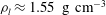
Near
 ${\it\xi}={\it\xi}_{N}$
, the thickness of the current obeys
${\it\xi}={\it\xi}_{N}$
, the thickness of the current obeys
 $$\begin{eqnarray}F\sim \left[\frac{9}{2}{\it\xi}_{N}^{2}\left(1-\frac{{\it\xi}}{{\it\xi}_{N}}\right)\right]^{1/3}\quad ({\it\xi}\rightarrow {\it\xi}_{N}),\end{eqnarray}$$
(Huppert Reference Huppert1982).
Assuming that the density difference
 $\mathscr{D}$
is bounded away from zero, the thickness of the lubricating layer obeys
$\mathscr{D}$
is bounded away from zero, the thickness of the lubricating layer obeys
 $$\begin{eqnarray}f\sim \left[\frac{9}{2}\frac{{\it\xi}_{L}^{2}}{\mathscr{M}\mathscr{D}}\left(1-\frac{{\it\xi}}{{\it\xi}_{L}}\right)\right]^{1/3}\quad ({\it\xi}\rightarrow {\it\xi}_{L}),\end{eqnarray}$$
and there is a discontinuity in upper surface slope, given by the jump condition
 $$\begin{eqnarray}[F^{\prime }]_{-}^{+}=-\frac{9}{4}\frac{{\it\xi}_{L}}{F^{2}}\quad ({\it\xi}={\it\xi}_{L}).\end{eqnarray}$$
Such a change of slope is seen in experiments, reported below.
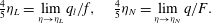
Figure 5. Similarity solutions and asymptotic results in axisymmetry. Solutions of (3.19)–(3.28) for the thicknesses of both currents are presented as solid curves. Asymptotic solutions (3.29) and (3.30) near the two fronts are presented as dashed bold curves. Parameter values used are
 $\mathscr{M}=100$
,
$\mathscr{M}=100$
,
 $\mathscr{D}=1$
and
$\mathscr{D}=1$
and
 $\mathscr{Q}=0.2$
.
$\mathscr{Q}=0.2$
.
The asymptotic solutions above were used as starting conditions in solving the ODEs (3.19)–(2.28) numerically using a similar shooting method as described in § 2.4. An illustrative solution of (3.19)–(2.28) is presented in figure 5 along with the asymptotic solutions (3.29) and (3.30). The solution of the full PDEs (3.8)–(3.16) is shown to converge to the similarity solution as
 $t\rightarrow \infty$
in figure 4.
$t\rightarrow \infty$
in figure 4.
4. Laboratory experiments
4.1. Experimental system
Experiments were carried out using simple Newtonian fluids. For the upper high-viscosity layer, we used golden syrup of density
 ${\it\rho}\approx 1.4~\text{g}~\text{cm}^{-3}$
and dynamic viscosity
${\it\rho}\approx 1.4~\text{g}~\text{cm}^{-3}$
and dynamic viscosity
 ${\it\mu}\approx 520{-}770~\text{g}~\text{cm}^{-1}~\text{s}^{-1}$
. For the lower, dense, low-viscosity layer, we used potassium carbonate solution, which can reach densities of up to around
${\it\mu}\approx 520{-}770~\text{g}~\text{cm}^{-1}~\text{s}^{-1}$
. For the lower, dense, low-viscosity layer, we used potassium carbonate solution, which can reach densities of up to around
 ${\it\rho}_{l}\approx 1.55~\text{g}~\text{cm}^{-3}$
and dynamic viscosity
${\it\rho}_{l}\approx 1.55~\text{g}~\text{cm}^{-3}$
and dynamic viscosity
 ${\it\mu}_{l}\approx 10^{-1}~\text{g}~\text{cm}^{-1}~\text{s}^{-1}$
. Even though
${\it\mu}_{l}\approx 10^{-1}~\text{g}~\text{cm}^{-1}~\text{s}^{-1}$
. Even though
 ${\it\mu}_{l}$
is small, the lubricating layer can be treated using the lubrication equations since its thickness is small enough that the corresponding reduced Reynolds number
${\it\mu}_{l}$
is small, the lubricating layer can be treated using the lubrication equations since its thickness is small enough that the corresponding reduced Reynolds number
 $$\begin{eqnarray}\mathit{Re}_{r}=\frac{Uh^{2}}{{\it\nu}_{l}L}\end{eqnarray}$$
is small. A typical value for our experiments after 1 s is
 $\mathit{Re}_{r}\sim 1$
, while after 100 s,
$\mathit{Re}_{r}\sim 1$
, while after 100 s,
 $\mathit{Re}_{r}\sim 10^{-2}$
. Here,
$\mathit{Re}_{r}\sim 10^{-2}$
. Here,
 $L\approx x_{L}$
is a characteristic horizontal length scale of the lubricating layer, and
$L\approx x_{L}$
is a characteristic horizontal length scale of the lubricating layer, and
 $U$
is its characteristic horizontal velocity scale.
$U$
is its characteristic horizontal velocity scale.
The experimental system is shown schematically in figure 6. The experiments began by releasing golden syrup at constant flux from the reservoir above a square glass sheet of
 $100~\text{cm}$
side length to form an axisymmetric viscous gravity current. The syrup was gravity-fed, and a constant head was maintained in the reservoir. To minimize the amount of air bubbles in the golden syrup as a result of entrainment, the reservoir head is maintained constant by immersing a solid body of known volume at a rate tuned by manual adjustment to keep the head maintained. The resulting flux of syrup is measured by comparing the immersed volume to the duration of the experiment. After a time
$100~\text{cm}$
side length to form an axisymmetric viscous gravity current. The syrup was gravity-fed, and a constant head was maintained in the reservoir. To minimize the amount of air bubbles in the golden syrup as a result of entrainment, the reservoir head is maintained constant by immersing a solid body of known volume at a rate tuned by manual adjustment to keep the head maintained. The resulting flux of syrup is measured by comparing the immersed volume to the duration of the experiment. After a time
 $\mathscr{T}$
, once the syrup had reached an appreciable radius, typically
$\mathscr{T}$
, once the syrup had reached an appreciable radius, typically
 $r_{N}\approx 20~\text{cm}$
, potassium carbonate solution was injected from below at constant volume flux by means of a syringe pump through a plastic tube to a 5 mm diameter nozzle fitted to a 6 mm diameter hole in the centre of the glass sheet. Before each experiment, care was taken to align the injection nozzle with the centre point of the golden syrup delivery tube to within 1 mm. This is needed in order to ensure that both currents spread axisymmetrically and concentrically.
$r_{N}\approx 20~\text{cm}$
, potassium carbonate solution was injected from below at constant volume flux by means of a syringe pump through a plastic tube to a 5 mm diameter nozzle fitted to a 6 mm diameter hole in the centre of the glass sheet. Before each experiment, care was taken to align the injection nozzle with the centre point of the golden syrup delivery tube to within 1 mm. This is needed in order to ensure that both currents spread axisymmetrically and concentrically.
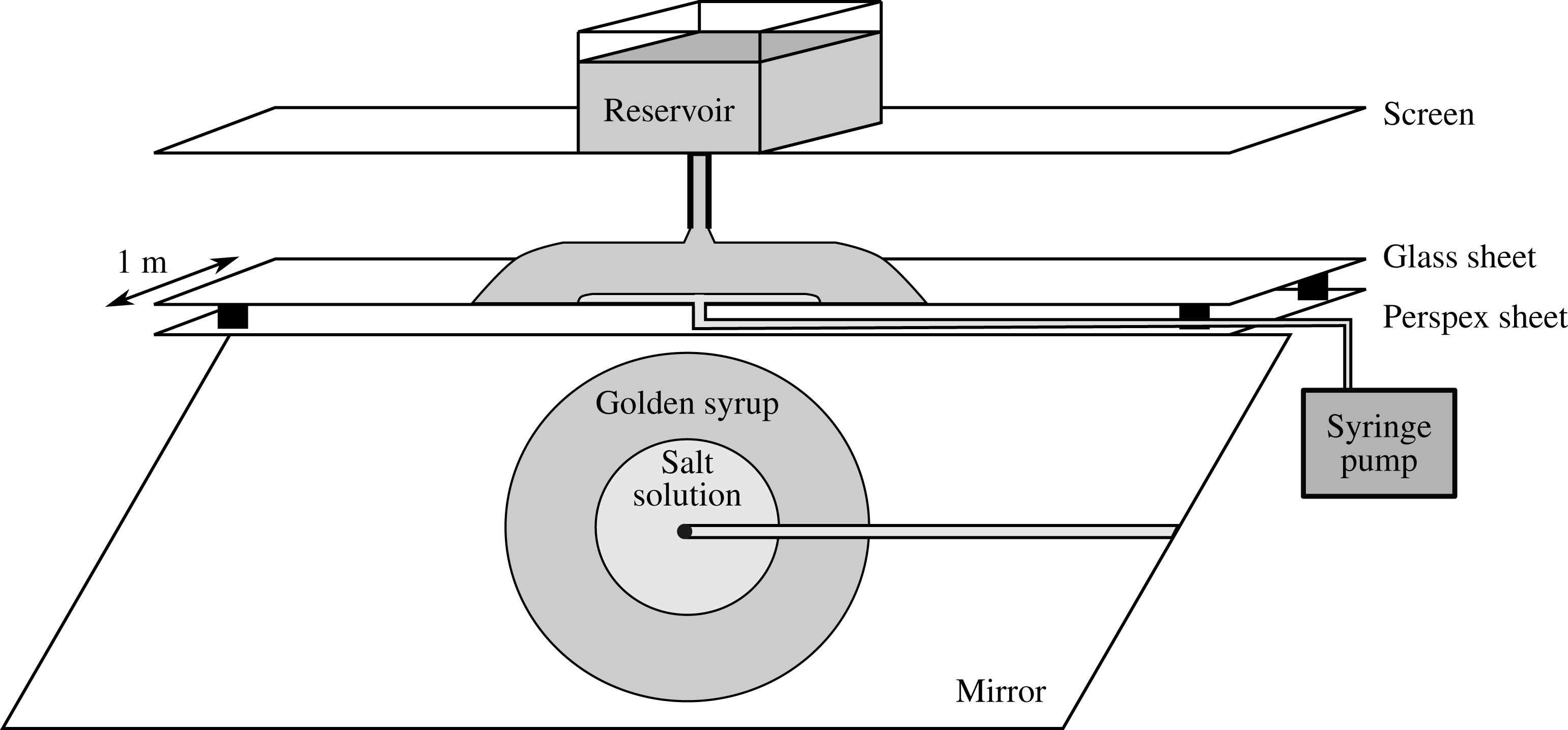
Figure 6. Schematic of our experimental set-up.
A major difficulty in our experiments that affected our measurements and the comparison with our theoretical predictions is the precise alignment of the injection nozzle and the golden syrup delivery tube. Other effects, such as the effect of surface tension between the two layers are negligible in our experiments. There may be contributions from diffusive mixing between the two layers and the possible existence of a thin film of syrup (
 $\ll 1~\text{mm}$
) between the lubricating layer and the glass sheet. However, these effects seem not to have been important in our experiments.
$\ll 1~\text{mm}$
) between the lubricating layer and the glass sheet. However, these effects seem not to have been important in our experiments.
The parameter values used in our experiments are recorded in table 1. The viscosity of golden syrup is strongly dependent on temperature. There were differences in viscosities caused by variations in temperature in different experiments and care was taken to measure the viscosity of golden syrup, using a falling-sphere method, before each experiment. We measured the viscosities of potassium carbonate solution using a U-tube viscometer, and its density by weight before each experiment. The density of the golden syrup was measured using a hydrometer.
Table 1. Parameter values used in our experiments.
We placed a mirror at 45° to the horizontal beneath the transparent perspex sheet to observe the evolution of the frontal positions of both currents, and used a digital camera to record the result in equal time increments. To visualize the underlying layer, the potassium carbonate solution was dyed green. When dissolved in water, potassium carbonate forms a strongly alkaline solution for which several traditional colorants that we tried are ineffective, as they form a suspension of solid particles that quickly separate from the solution. For better stability, a soap dye suitable for higher values of pH was used.
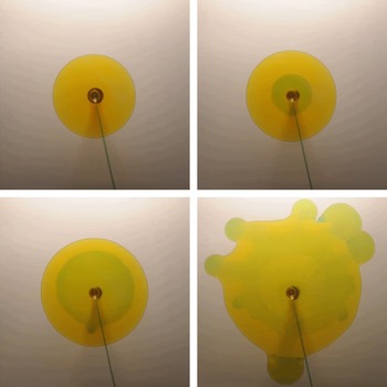
Figure 7. Bottom view of experiment D at
 $t=0,60,180,420$
s after injection of salt solution. The full experiment is shown in supplementary movie 1 (http://dx.doi.org/10.1017/jfm.2015.30).
$t=0,60,180,420$
s after injection of salt solution. The full experiment is shown in supplementary movie 1 (http://dx.doi.org/10.1017/jfm.2015.30).
4.2. Experimental results
A sequence of photographs showing one of our experiments from the bottom view mirror is presented in figure 7. The first photograph is taken before the injection of potassium carbonate solution, and consists of golden syrup only, spreading axisymmetrically. The next three photographs are taken after initiating the flow of the lower layer. Here, both the upper and lower currents spread more or less axisymmetrically until the edge of the less viscous fluid (dyed green) begins to undergo a fingering instability. The first appearance of a finger occurs after roughly 120 s after injection of the less viscous fluid. Note that there is a slight offset in the alignment of the currents, and the finger formed at the point on the outer edge of the less viscous fluid that is closest to the source. By analysing the bottom-view photographs of all our experiments, we deduce that the structure of the break in axisymmetry is sensitive to how precisely the bottom injection nozzle is aligned with the golden syrup delivery tube above. Our theory corresponds to the part of our experiments before the instability. We record frontal positions as an average along four radial lines from the injection nozzle.
Given the time delay between the initiation of flow of the two fluids at the start of our experiments, the similarity solution of § 3.4 does not apply. The measured frontal positions are compared with solutions of the full system of PDEs (3.8)–(3.16a,b
) in figure 9. There is mostly good agreement between our experiments and theoretical predictions for the whole range of parameter values used and recorded in table 1. Our experimental parameters were in a range of large
 $\mathscr{M}$
and small
$\mathscr{M}$
and small
 $\mathscr{Q}$
, similar to the geophysical setting. The experimental values of the viscosity ratios
$\mathscr{Q}$
, similar to the geophysical setting. The experimental values of the viscosity ratios
 $\mathscr{M}$
ranged from
$\mathscr{M}$
ranged from
 $5180$
to
$5180$
to
 $6680$
. We also altered fluxes of both layers, giving flux ratios
$6680$
. We also altered fluxes of both layers, giving flux ratios
 $\mathscr{Q}$
in the range 0.14–0.30, and kept our density difference
$\mathscr{Q}$
in the range 0.14–0.30, and kept our density difference
 $\mathscr{D}$
around 0.09, which is close to the ice–water density difference. Unlike the parameter
$\mathscr{D}$
around 0.09, which is close to the ice–water density difference. Unlike the parameter
 $\mathscr{D}$
and time delay
$\mathscr{D}$
and time delay
 $\mathscr{T}$
, which can be readily prescribed, the values of
$\mathscr{T}$
, which can be readily prescribed, the values of
 $\mathscr{M}$
and
$\mathscr{M}$
and
 $\mathscr{Q}$
vary between experiments owing to temperature and concentration differences, which affects the viscosity and the resultant gravity-fed flux of syrup.
$\mathscr{Q}$
vary between experiments owing to temperature and concentration differences, which affects the viscosity and the resultant gravity-fed flux of syrup.
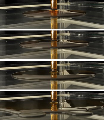
Figure 8. Side view of experiment D at
 $t=0,60,180,420$
s after injection of salt solution. The full experiment is shown in supplementary movie 2.
$t=0,60,180,420$
s after injection of salt solution. The full experiment is shown in supplementary movie 2.
Figure 9 shows a comparison of our experimental data to the solution of the full system of PDEs (3.8)–(3.16). The discrete symbols correspond to measured values of
 $r_{L}$
(unfilled circles) and
$r_{L}$
(unfilled circles) and
 $r_{N}$
(filled circles), while the dashed and solid lines are our solutions to (3.8)–(3.16). There is good agreement for each of our experiments, giving confidence in the assumptions of our theory.
$r_{N}$
(filled circles), while the dashed and solid lines are our solutions to (3.8)–(3.16). There is good agreement for each of our experiments, giving confidence in the assumptions of our theory.
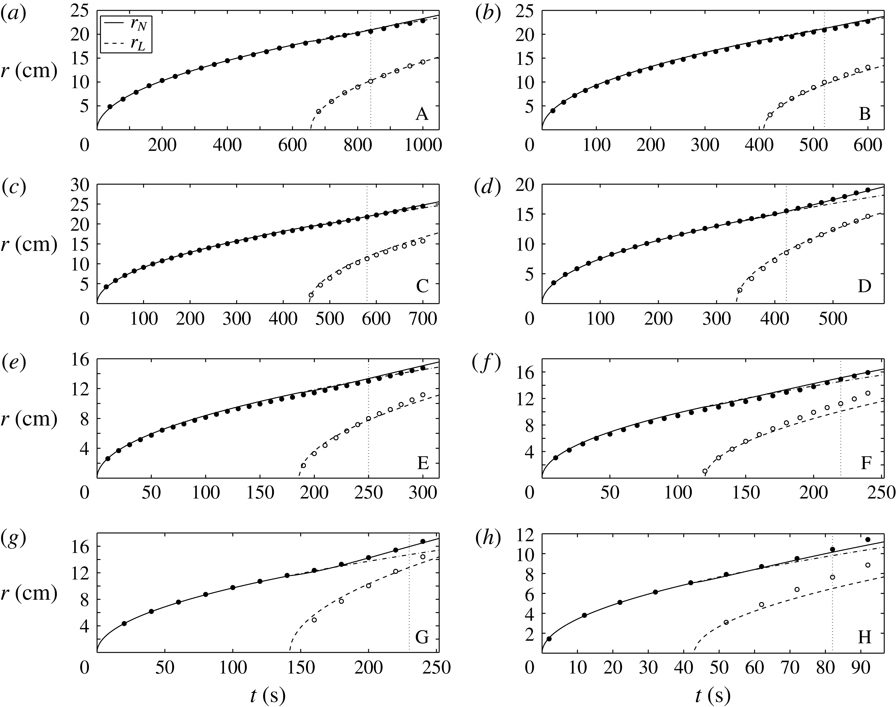
Figure 9. Comparison of our experimental data for experiments A–H for
 $r_{N}$
( filled symbols) and
$r_{N}$
( filled symbols) and
 $r_{L}$
(open symbols) to solutions for
$r_{L}$
(open symbols) to solutions for
 $r_{N}$
(solid) and
$r_{N}$
(solid) and
 $r_{L}$
(dashed) of the full system of PDEs (3.8)–(3.16) for axisymmetric spreading. The dash-dot curves show
$r_{L}$
(dashed) of the full system of PDEs (3.8)–(3.16) for axisymmetric spreading. The dash-dot curves show
 $r_{N}$
as a function of
$r_{N}$
as a function of
 $t$
in the unlubricated case. The vertical dotted lines indicate the time at which there is a first sign of a fingering instability in the experiments.
$t$
in the unlubricated case. The vertical dotted lines indicate the time at which there is a first sign of a fingering instability in the experiments.

Figure 10. Experimental values for
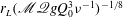 $r_{L}(\mathscr{M}\mathscr{Q}gQ_{0}^{3}{\it\nu}^{-1})^{-1/8}$
versus time. The solid line is a least-squares power-law fit.
$r_{L}(\mathscr{M}\mathscr{Q}gQ_{0}^{3}{\it\nu}^{-1})^{-1/8}$
versus time. The solid line is a least-squares power-law fit.
Figure 10 shows the radial position of the lubricant front for all experiments, normalized by
 $(\mathscr{M}\mathscr{Q}gq_{0}^{3}{\it\nu}^{-1})^{1/8}$
on logarithmically scaled axes. The data fall together on a single line, given by the least-squares fit
$(\mathscr{M}\mathscr{Q}gq_{0}^{3}{\it\nu}^{-1})^{1/8}$
on logarithmically scaled axes. The data fall together on a single line, given by the least-squares fit
 $$\begin{eqnarray}r_{L}=(0.27\pm 0.02)(\mathscr{M}\mathscr{Q}gQ_{0}^{3}{\it\nu}^{-1})^{1/8}t^{0.52\pm 0.02}.\end{eqnarray}$$
The line (4.2) scales like the radial extent of a self-similar underlying current of § 5.3. The deviations originate mainly from the fact that our experimental currents are not self similar because of the non-zero time delay
 $\mathscr{T}$
, while the scaling corresponds to self-similar currents.
$\mathscr{T}$
, while the scaling corresponds to self-similar currents.
A sequence of photographs of an angled side view of one of our experiments is shown in figure 8. There is a noticeable discontinuity in slope at
 $r_{L}$
and a flat horizontal surface height in the lubricated region, similar to our theoretical prediction shown in figure 4(a) with side-profile thicknesses with similar parameter values.
$r_{L}$
and a flat horizontal surface height in the lubricated region, similar to our theoretical prediction shown in figure 4(a) with side-profile thicknesses with similar parameter values.
5. Flow regimes
The mathematical models developed in the previous sections in two-dimensional and axisymmetric geometries describe a general class of gravity currents spreading inside of gravity currents of different fluid properties. The flow depends on three dimensionless parameters and its behaviour changes in different parameter regimes. In this section, we extract the relevant scalings and important physical balances in the different parameter regimes. We focus on large viscosity ratios
 $\mathscr{M}$
, as in the geophysical setting, but also compare with the case of small
$\mathscr{M}$
, as in the geophysical setting, but also compare with the case of small
 $\mathscr{M}$
.
$\mathscr{M}$
.
We lead the discussion by example of our two-dimensional, self-similar model. Results for the axisymmetric case are summarized in table 2. As can be seen from analysing the order of the terms in (2.38)–(2.44), the mechanisms driving the flow change depending on the choice of parameters. In what follows, we restrict attention to
 $\mathscr{D}$
fixed and bounded away from zero, unless otherwise stated. Unless otherwise stated, we also concentrate on the part of the lubricated region that is bounded away from its nose. Near its nose, the lower film always spreads as a result of its own weight (see §§ 2.4.1 and 3.4.1).
$\mathscr{D}$
fixed and bounded away from zero, unless otherwise stated. Unless otherwise stated, we also concentrate on the part of the lubricated region that is bounded away from its nose. Near its nose, the lower film always spreads as a result of its own weight (see §§ 2.4.1 and 3.4.1).
The
 $(\mathscr{Q},\mathscr{M})$
parameter space consists of four regimes, pictured in figure 11. Each regime is discussed in a separate subsection, below. We start by considering
$(\mathscr{Q},\mathscr{M})$
parameter space consists of four regimes, pictured in figure 11. Each regime is discussed in a separate subsection, below. We start by considering
 $\mathscr{M}\gg 1$
and the two extreme cases of small and large
$\mathscr{M}\gg 1$
and the two extreme cases of small and large
 $\mathscr{Q}$
.
$\mathscr{Q}$
.
Figure 11. Regimes (I)–(IV) in parameter space for two-dimensional currents. Here
 $\mathscr{D}$
is held fixed and bounded away from zero.
$\mathscr{D}$
is held fixed and bounded away from zero.
5.1. Regime (I): classical spreading of the more viscous fluid
In the limit
 $\mathscr{M}\mathscr{Q}\ll 1$
and
$\mathscr{M}\mathscr{Q}\ll 1$
and
 $\mathscr{Q}\ll \mathscr{M}^{3}$
and with the scalings
$\mathscr{Q}\ll \mathscr{M}^{3}$
and with the scalings
 $$\begin{eqnarray}{\it\eta}_{L}=O(\mathscr{M}\mathscr{Q})^{1/2},\quad {\it\eta}_{N}=O(1),\quad f=O\left(\frac{\mathscr{Q}}{\mathscr{M}}\right)^{1/2},\quad F,F^{\prime }=O(1),\end{eqnarray}$$
the governing equations for
 $0\leqslant {\it\eta}\leqslant {\it\eta}_{L}$
reduce to
$0\leqslant {\it\eta}\leqslant {\it\eta}_{L}$
reduce to
 $$\begin{eqnarray}\displaystyle & \displaystyle \frac{1}{5}f-\frac{4}{5}{\it\eta}f^{\prime }=\frac{\mathscr{M}}{2}(\,f^{2}FF^{\prime })^{\prime }, & \displaystyle\end{eqnarray}$$
 $$\begin{eqnarray}\displaystyle & \displaystyle 1=-{\textstyle \frac{1}{3}}F^{3}F^{\prime }. & \displaystyle\end{eqnarray}$$
In two-dimensional geometry, there is also a sub-regime with
 $\mathscr{M}^{3}\ll \mathscr{Q}\ll \mathscr{M}$
in which the gravitational spreading of the lower layer becomes important and (5.2) is replaced by
$\mathscr{M}^{3}\ll \mathscr{Q}\ll \mathscr{M}$
in which the gravitational spreading of the lower layer becomes important and (5.2) is replaced by
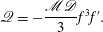 $$\begin{eqnarray}\mathscr{Q}=-\frac{\mathscr{M}\mathscr{D}}{3}f^{3}f^{\prime }.\end{eqnarray}$$
Table 2. Scalings in two-dimensional and axisymmetric settings.
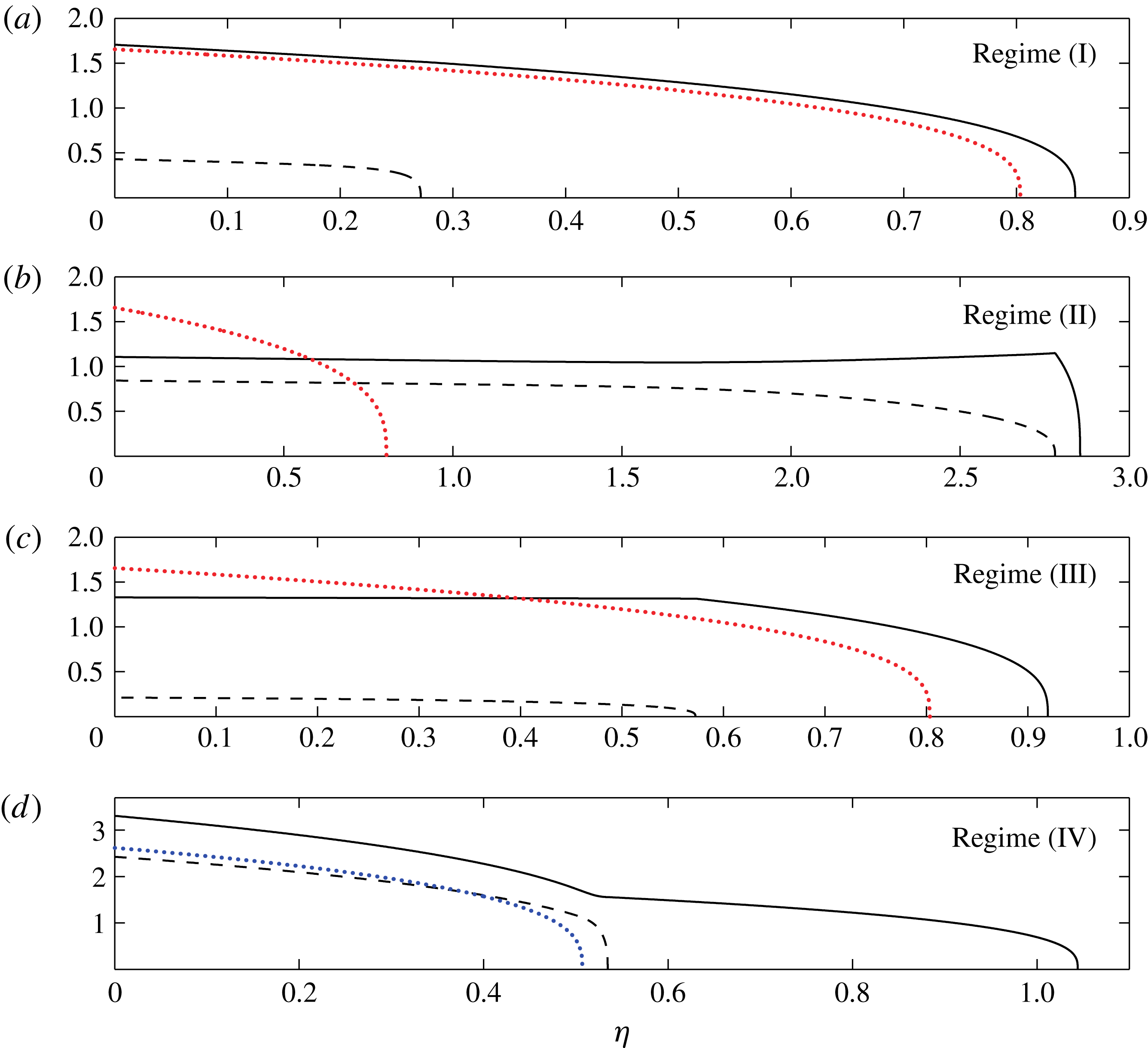
Figure 12. Profile thicknesses of two-dimensional two-layer gravity currents in similarity coordinates for a range of different parameters with
 $\mathscr{D}=1$
fixed. Upper surface heights are solid and interfacial heights are dashed. The dotted (red online) curves in (a–c) are the surface heights that the upper fluid would have if the lower fluid were not present. The dotted (blue online) curve in (d) is the surface height that the lower fluid would have if the upper fluid were not present. The parameter values used are
$\mathscr{D}=1$
fixed. Upper surface heights are solid and interfacial heights are dashed. The dotted (red online) curves in (a–c) are the surface heights that the upper fluid would have if the lower fluid were not present. The dotted (blue online) curve in (d) is the surface height that the lower fluid would have if the upper fluid were not present. The parameter values used are
 $\mathscr{M}=1$
,
$\mathscr{M}=1$
,
 $\mathscr{Q}=0.1$
in (a),
$\mathscr{Q}=0.1$
in (a),
 $\mathscr{M}=100$
,
$\mathscr{M}=100$
,
 $\mathscr{Q}=2$
in (b),
$\mathscr{Q}=2$
in (b),
 $\mathscr{M}=100$
,
$\mathscr{M}=100$
,
 $\mathscr{Q}=0.1$
in (c) and
$\mathscr{Q}=0.1$
in (c) and
 $\mathscr{M}=0.05$
and
$\mathscr{M}=0.05$
and
 $\mathscr{Q}=1$
in (d). (a–d) correspond to regimes (I)–(IV), respectively.
$\mathscr{Q}=1$
in (d). (a–d) correspond to regimes (I)–(IV), respectively.
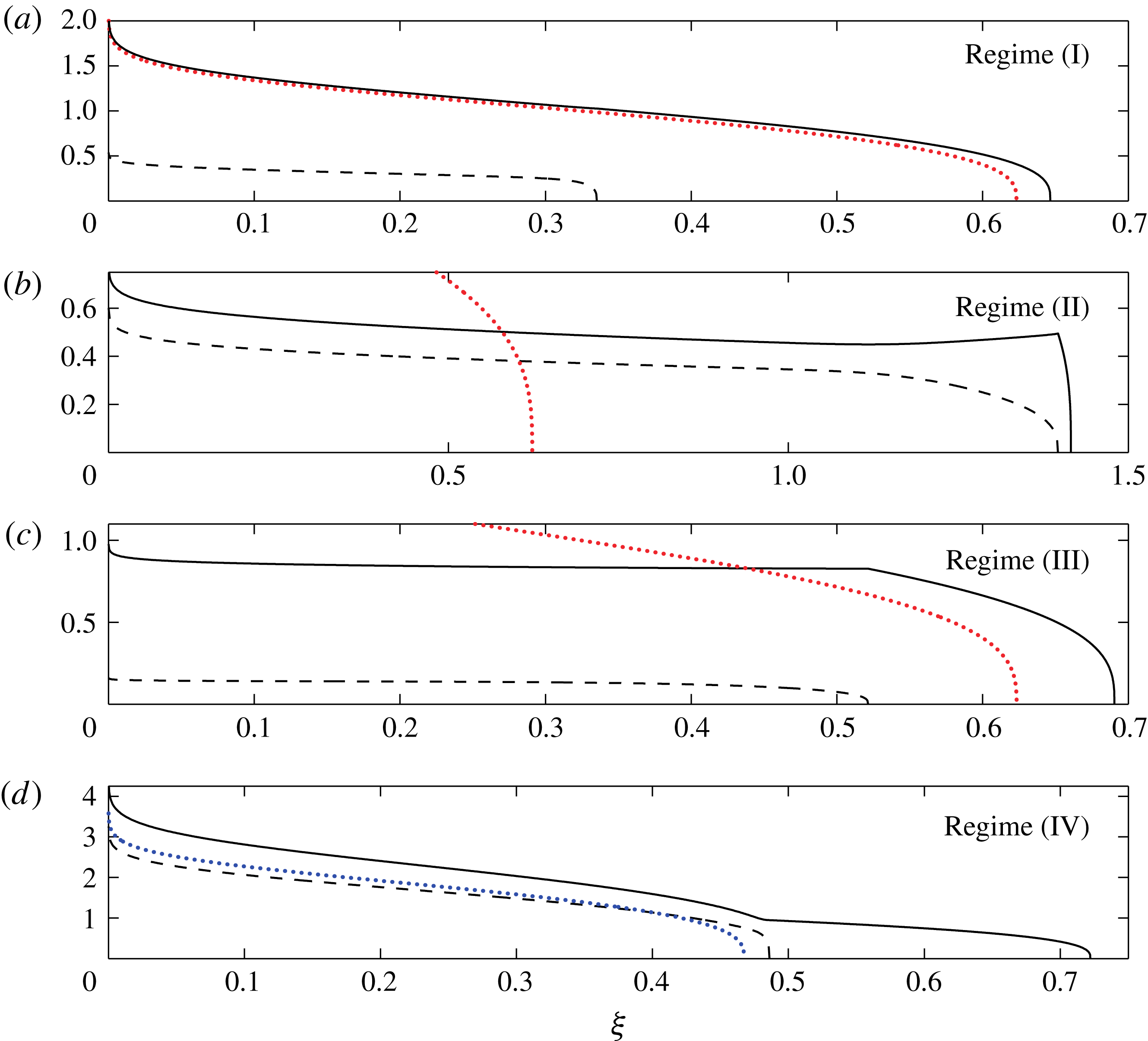
Figure 13. Profile thicknesses of axisymmetric two-layer gravity currents in similarity coordinates for a range of different parameters with
 $\mathscr{D}=1$
fixed. Upper surface heights are solid and interfacial heights are dashed. The dotted (red online) curves in (a–c) are the surface heights that the upper fluid would have if the lower fluid were not present. The dotted (blue online) curve in (d) is the surface height that the lower fluid would have if the upper fluid were not present. The parameter values used are
$\mathscr{D}=1$
fixed. Upper surface heights are solid and interfacial heights are dashed. The dotted (red online) curves in (a–c) are the surface heights that the upper fluid would have if the lower fluid were not present. The dotted (blue online) curve in (d) is the surface height that the lower fluid would have if the upper fluid were not present. The parameter values used are
 $\mathscr{M}=1$
,
$\mathscr{M}=1$
,
 $\mathscr{Q}=0.1$
in (a),
$\mathscr{Q}=0.1$
in (a),
 $\mathscr{M}=100$
,
$\mathscr{M}=100$
,
 $\mathscr{Q}=2$
in (b),
$\mathscr{Q}=2$
in (b),
 $\mathscr{M}=100$
,
$\mathscr{M}=100$
,
 $\mathscr{Q}=0.1$
in (c), and
$\mathscr{Q}=0.1$
in (c), and
 $\mathscr{M}=0.05$
and
$\mathscr{M}=0.05$
and
 $\mathscr{Q}=1$
in (d). (a–d) correspond to regimes (I)–(IV), respectively.
$\mathscr{Q}=1$
in (d). (a–d) correspond to regimes (I)–(IV), respectively.
Profiles of the lower and upper currents in the limit
 $\mathscr{M}\mathscr{Q}\ll 1$
and
$\mathscr{M}\mathscr{Q}\ll 1$
and
 $\mathscr{Q}\ll \mathscr{M}^{3}$
are shown in figure 12(a) for the two-dimensional case and in figure 13(a) for the axisymmetric case. Note that the lubricating layer is very thin when
$\mathscr{Q}\ll \mathscr{M}^{3}$
are shown in figure 12(a) for the two-dimensional case and in figure 13(a) for the axisymmetric case. Note that the lubricating layer is very thin when
 $\mathscr{M}$
is large, so we have taken
$\mathscr{M}$
is large, so we have taken
 $\mathscr{M}=1$
for better visibility. In both figures, the surface heights of the upper currents are shown as solid curves and the interfacial heights between the upper and lower currents are shown as dashed lines. The dotted (red online) curve for both geometries is the side profile thickness of a classical no-slip current, with fluid properties corresponding to the upper more viscous layer. The solid curves and dotted (red online) curves are indeed close to one another in both geometries, confirming that the presence of the underlying layer has a small effect on the upper fluid.
$\mathscr{M}=1$
for better visibility. In both figures, the surface heights of the upper currents are shown as solid curves and the interfacial heights between the upper and lower currents are shown as dashed lines. The dotted (red online) curve for both geometries is the side profile thickness of a classical no-slip current, with fluid properties corresponding to the upper more viscous layer. The solid curves and dotted (red online) curves are indeed close to one another in both geometries, confirming that the presence of the underlying layer has a small effect on the upper fluid.
5.2. Regime (II): spreading driven by the underlying fluid
Another scenario can be attained by taking
 $\mathscr{Q}\gg 1$
with
$\mathscr{Q}\gg 1$
with
 $\mathscr{M}\mathscr{Q}^{2}\gg 1$
. With the scalings
$\mathscr{M}\mathscr{Q}^{2}\gg 1$
. With the scalings
 $$\begin{eqnarray}{\it\eta}_{L},{\it\eta}_{N}=O(\mathscr{M}\mathscr{Q}^{3})^{1/5},\quad f,F=O\left(\frac{\mathscr{Q}^{2}}{\mathscr{M}}\right)^{1/5}\quad \text{and}\quad \frac{F-f}{f}=O\left(\frac{1}{\mathscr{Q}}\right)\!,\end{eqnarray}$$
the governing equations for
 $0\leqslant {\it\eta}\leqslant {\it\eta}_{L}$
reduce to
$0\leqslant {\it\eta}\leqslant {\it\eta}_{L}$
reduce to
 $$\begin{eqnarray}\displaystyle & \displaystyle \frac{1}{5}f-\frac{4}{5}{\it\eta}f^{\prime }=\frac{\mathscr{M}(\mathscr{D}+1)}{3}(\,f^{3}f^{\prime })^{\prime }, & \displaystyle\end{eqnarray}$$
 $$\begin{eqnarray}\displaystyle & \displaystyle \frac{1}{5}(F-f)-\frac{4}{5}{\it\eta}(F-f)^{\prime }=\frac{\mathscr{M}(\mathscr{D}+1)}{2}[f^{2}(F-f)f^{\prime }]^{\prime }. & \displaystyle\end{eqnarray}$$
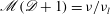 $\mathscr{M}(\mathscr{D}+1)={\it\nu}/{\it\nu}_{l}$
is the kinematic viscosity ratio between the two layers.
$\mathscr{M}(\mathscr{D}+1)={\it\nu}/{\it\nu}_{l}$
is the kinematic viscosity ratio between the two layers.
Figures 12(b) and 13(b) show side-profile thicknesses as functions of
 $x$
and
$x$
and
 $r$
of both the upper and lower currents in two dimensions and in axisymmetric geometry. The plug-like upper layer, lubricated by a large amount of fluid underneath it, behaves very differently from a classical no-slip current. This can be seen by the stark contrast between the surface height of the more viscous current (solid curve) and the thickness of a classical no-slip current of the same fluid properties, shown as a dotted red curve in figures 12(b) and 13(b) for both geometries. The upper fluid effectively forms a thin viscous skin on the lower layer, which otherwise behaves similarly to a classical gravity current.
$r$
of both the upper and lower currents in two dimensions and in axisymmetric geometry. The plug-like upper layer, lubricated by a large amount of fluid underneath it, behaves very differently from a classical no-slip current. This can be seen by the stark contrast between the surface height of the more viscous current (solid curve) and the thickness of a classical no-slip current of the same fluid properties, shown as a dotted red curve in figures 12(b) and 13(b) for both geometries. The upper fluid effectively forms a thin viscous skin on the lower layer, which otherwise behaves similarly to a classical gravity current.
As the interfacial slip velocity of the upper fluid exceeds the velocities of a no-slip current of the same fluid properties, excess high viscosity fluid may accumulate near the lubricating front. Near this front, the resulting surface height has a slope that is reversed with respect to the upstream end. This can be seen in figure 12(b) in two dimensions and in figure 13(b) in axisymmetric geometry. There is an evident reversal of surface height slope in both geometries. A surface slope reversal may be surprising at first, as it indicates that the gravitational spreading of the upper current counteracts its motion. Such a current is instead driven by the boundary motion generated at the interface between the two fluids, as a result of the gravitational spreading of the lower current. It is the lower current that generates motion, and the upper current gets viscously dragged along with it.
5.3. Regime (III): transitional thin lubricating layer
There is a transitional region
 $1/\mathscr{M}\ll \mathscr{Q}\ll 1$
between regimes (I) and (II), in which the lubricant deforms under hydrostatic pressure gradients established in the overlying, high-viscosity current. With the scalings
$1/\mathscr{M}\ll \mathscr{Q}\ll 1$
between regimes (I) and (II), in which the lubricant deforms under hydrostatic pressure gradients established in the overlying, high-viscosity current. With the scalings
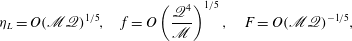 $$\begin{eqnarray}{\it\eta}_{L}=O(\mathscr{M}\mathscr{Q})^{1/5},\quad \displaystyle f=O\left(\frac{\mathscr{Q}^{4}}{\mathscr{M}}\right)^{1/5},\quad F=O(\mathscr{M}\mathscr{Q})^{-1/5},\end{eqnarray}$$
the governing equations for
 $0\leqslant {\it\eta}\leqslant {\it\eta}_{L}$
reduce to
$0\leqslant {\it\eta}\leqslant {\it\eta}_{L}$
reduce to
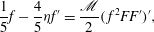 $$\begin{eqnarray}\displaystyle & \displaystyle \frac{1}{5}f-\frac{4}{5}{\it\eta}f^{\prime }=\frac{\mathscr{M}}{2}(\,f^{2}FF^{\prime })^{\prime }, & \displaystyle\end{eqnarray}$$
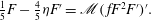 $$\begin{eqnarray}\displaystyle & {\textstyle \frac{1}{5}}F-{\textstyle \frac{4}{5}}{\it\eta}F^{\prime }=\mathscr{M}(\,fF^{2}F^{\prime })^{\prime }. & \displaystyle\end{eqnarray}$$
 $r=0$
. The height of the lower layer is also flat in most of the lubricated region away from the origin, the exception being at the nose of the lubricating front, where the lower layer is driven by its spreading under gravity. Apart from this vicinity, the thicknesses of both currents are largely flat in the lubricated region.
$r=0$
. The height of the lower layer is also flat in most of the lubricated region away from the origin, the exception being at the nose of the lubricating front, where the lower layer is driven by its spreading under gravity. Apart from this vicinity, the thicknesses of both currents are largely flat in the lubricated region.
Profiles of the upper and lower currents are compared against the thickness of a classical current in figures 12(c) and 13(c) for both geometries. As can be seen in these figures, the presence of the low-viscosity underlying layer influences the shape of the overlying viscous current in this limit as well. Note that our experiments fall generally within regime (III).
5.4. Regime (IV): low-viscosity thin film coating a more viscous current
Our theory can also be applied to low viscosity ratios. We consider the limit
 $\mathscr{M}\ll \mathscr{Q}$
and
$\mathscr{M}\ll \mathscr{Q}$
and
 $\mathscr{M}\mathscr{Q}^{2}\ll 1$
(which implies
$\mathscr{M}\mathscr{Q}^{2}\ll 1$
(which implies
 $\mathscr{M}\ll 1$
). With the scales
$\mathscr{M}\ll 1$
). With the scales
 $$\begin{eqnarray}{\it\eta}_{L}=O(\mathscr{M}\mathscr{Q}^{3})^{1/5},\quad {\it\eta}_{N}=O(1),\quad f=O\left(\frac{\mathscr{Q}^{2}}{\mathscr{M}}\right)^{1/5},\quad \frac{F-f}{f}=O\left(\frac{\mathscr{M}}{\mathscr{Q}}\right)^{1/3},\end{eqnarray}$$
the governing equations for
 $0\leqslant {\it\eta}\leqslant {\it\eta}_{L}$
reduce to
$0\leqslant {\it\eta}\leqslant {\it\eta}_{L}$
reduce to
 $$\begin{eqnarray}\displaystyle & \displaystyle \frac{1}{5}f-\frac{4}{5}{\it\eta}f^{\prime }=\frac{\mathscr{M}(\mathscr{D}+1)}{3}(\,f^{3}f^{\prime })^{\prime }, & \displaystyle\end{eqnarray}$$
 $$\begin{eqnarray}\displaystyle & -{\textstyle \frac{1}{3}}(F-f)^{3}F^{\prime }=1. & \displaystyle\end{eqnarray}$$
Figures 12(d) and 13(d) show the surface heights and interfacial heights between the two fluids in this limit, in a two-dimensional and an axisymmetric setting. The upper film is ten times less viscous than the main current in both of these figures, and runs off ahead of the main, lower current, to greater distance than it would if the more viscous lower fluid where not there. The dotted (blue online) curves in both figures show the shape of a classical current formed by the more viscous underlying fluid if it were not coated by a less viscous thin film above. It can be seen in these figures, unsurprisingly, that the shape of a viscous gravity current is not greatly affected by the presence of a less viscous thin surface film coating it from above.
Figure 14. (a,b) Front positions and (c,d) source thicknesses of two dimensional currents on regular and log–log axes, all versus flux ratio. Parameter values used are
 $\mathscr{M}=50$
and
$\mathscr{M}=50$
and
 $\mathscr{D}=1$
, corresponding to regimes (I)–(III). The solid (red online) line in (a,b) corresponds to the extent of the upper more viscous current, if the lower less viscous layer were not present. The solid (red online) line in (c) corresponds to the thickness of the upper more viscous current if the lower less viscous layer were not present. The power laws (5.1), (5.5), and (5.8) for
$\mathscr{D}=1$
, corresponding to regimes (I)–(III). The solid (red online) line in (a,b) corresponds to the extent of the upper more viscous current, if the lower less viscous layer were not present. The solid (red online) line in (c) corresponds to the thickness of the upper more viscous current if the lower less viscous layer were not present. The power laws (5.1), (5.5), and (5.8) for
 ${\it\eta}_{L}$
and
${\it\eta}_{L}$
and
 $f_{0}$
with respect to
$f_{0}$
with respect to
 $\mathscr{Q}$
are shown as triangles.
$\mathscr{Q}$
are shown as triangles.
Figure 15. (a) Front positions and (b) source thicknesses of two dimensional currents on log–log axes versus viscosity ratio, for
 $\mathscr{Q}=0.001$
and
$\mathscr{Q}=0.001$
and
 $\mathscr{D}=1$
, corresponding to regime (I). The power laws (5.1a−d
) for
$\mathscr{D}=1$
, corresponding to regime (I). The power laws (5.1a−d
) for
 ${\it\eta}_{L}$
and
${\it\eta}_{L}$
and
 $f_{0}$
with respect to
$f_{0}$
with respect to
 $\mathscr{M}$
are shown as triangles.
$\mathscr{M}$
are shown as triangles.
5.5. Variation across regimes
Figure 14(a) shows the frontal positions
 ${\it\eta}_{N}$
and
${\it\eta}_{N}$
and
 ${\it\eta}_{L}$
of two-dimensional currents as functions of
${\it\eta}_{L}$
of two-dimensional currents as functions of
 $\mathscr{Q}$
with
$\mathscr{Q}$
with
 $\mathscr{M}=50$
and
$\mathscr{M}=50$
and
 $\mathscr{D}=1$
fixed. We see that
$\mathscr{D}=1$
fixed. We see that
 ${\it\eta}_{L}\rightarrow 0$
(the extent of the lubricant decreases to 0) as
${\it\eta}_{L}\rightarrow 0$
(the extent of the lubricant decreases to 0) as
 $\mathscr{Q}\rightarrow 0$
. This is expected, as
$\mathscr{Q}\rightarrow 0$
. This is expected, as
 $\mathscr{Q}=0$
corresponds to a classical viscous no-slip current without any lubricant present. The convergence occurs in a small inner region near
$\mathscr{Q}=0$
corresponds to a classical viscous no-slip current without any lubricant present. The convergence occurs in a small inner region near
 $\mathscr{Q}=0$
. We subdivide the range of
$\mathscr{Q}=0$
. We subdivide the range of
 $\mathscr{Q}$
into three intervals, corresponding to the three parameter regimes described above, and show the resulting frontal positions on logarithmically scaled axes in figure 14(b). The inner region near
$\mathscr{Q}$
into three intervals, corresponding to the three parameter regimes described above, and show the resulting frontal positions on logarithmically scaled axes in figure 14(b). The inner region near
 $\mathscr{Q}=0$
corresponds to the limit in which the more viscous fluid spreads under its own weight and generates boundary motion which drives the lubricating layer. In each of the three parameter regimes, separated by vertical dotted lines, the extent
$\mathscr{Q}=0$
corresponds to the limit in which the more viscous fluid spreads under its own weight and generates boundary motion which drives the lubricating layer. In each of the three parameter regimes, separated by vertical dotted lines, the extent
 ${\it\eta}_{L}$
of the lubricated region follows a different power law indicated by the triangle side lengths corresponding to the slope of the lines. The lubricant extent in the large
${\it\eta}_{L}$
of the lubricated region follows a different power law indicated by the triangle side lengths corresponding to the slope of the lines. The lubricant extent in the large
 $\mathscr{Q}$
parameter regime varies the most when
$\mathscr{Q}$
parameter regime varies the most when
 $\mathscr{Q}$
is large, and increases towards
$\mathscr{Q}$
is large, and increases towards
 ${\it\eta}_{N}$
, making the lubricated region dominate the system as
${\it\eta}_{N}$
, making the lubricated region dominate the system as
 $\mathscr{Q}\rightarrow \infty$
.
$\mathscr{Q}\rightarrow \infty$
.
We now compare the extent and thickness of lubricated gravity currents to that of a classical current. The solid (red online) line in figures 14(a,b) shows the extent
 ${\it\eta}_{N}$
of the more viscous current if the low-viscosity underlying layer were not present. Unsurprisingly, the extent of the lubricated current reaches the extent of the no-slip classical current as
${\it\eta}_{N}$
of the more viscous current if the low-viscosity underlying layer were not present. Unsurprisingly, the extent of the lubricated current reaches the extent of the no-slip classical current as
 $\mathscr{Q}\rightarrow 0$
, as seen in figure 14(a,b). As
$\mathscr{Q}\rightarrow 0$
, as seen in figure 14(a,b). As
 $\mathscr{Q}$
increases, the extent
$\mathscr{Q}$
increases, the extent
 ${\it\eta}_{N}$
becomes much larger than it would have been without the lubricant.
${\it\eta}_{N}$
becomes much larger than it would have been without the lubricant.
Figure 14(c,d) show the surface height and interfacial height between the two fluids at the source. The solid (red online) line shows the thickness of the more viscous current if the less-viscous layer were not present. The surface height of the lubricated current reaches that of the no-slip classical current as
 $\mathscr{Q}\rightarrow 0$
, as expected. Also, as expected, the lubricant thickness decreases to
$\mathscr{Q}\rightarrow 0$
, as expected. Also, as expected, the lubricant thickness decreases to
 $0$
as
$0$
as
 $\mathscr{Q}\rightarrow 0$
, corresponding to there being no lubricant at all. It can be seen that as the flux of lubricant increases, the more viscous fluid thins, with its surface height decreasing as
$\mathscr{Q}\rightarrow 0$
, corresponding to there being no lubricant at all. It can be seen that as the flux of lubricant increases, the more viscous fluid thins, with its surface height decreasing as
 $\mathscr{Q}$
increases, until the surface height starts to increase because of its displacement caused by the large amount of low-viscosity fluid underneath. The range of
$\mathscr{Q}$
increases, until the surface height starts to increase because of its displacement caused by the large amount of low-viscosity fluid underneath. The range of
 $\mathscr{Q}$
where the increase in surface height becomes apparent corresponds to regime (II), in which the low-viscosity underlying current drives the flow, and the more viscous fluid acts as a viscous skin on the low-viscosity fluid below.
$\mathscr{Q}$
where the increase in surface height becomes apparent corresponds to regime (II), in which the low-viscosity underlying current drives the flow, and the more viscous fluid acts as a viscous skin on the low-viscosity fluid below.
The triangle side lengths in figure 14 confirm the power law scalings (5.1), (5.5) and (5.8) for
 ${\it\eta}_{L}$
and
${\it\eta}_{L}$
and
 $f_{0}$
with respect to
$f_{0}$
with respect to
 $\mathscr{Q}$
. Figure 15 shows the front positions and source thicknesses of both layers as functions of
$\mathscr{Q}$
. Figure 15 shows the front positions and source thicknesses of both layers as functions of
 $\mathscr{M}$
within regime (I), and confirms the power law scalings (5.1) for
$\mathscr{M}$
within regime (I), and confirms the power law scalings (5.1) for
 ${\it\eta}_{L}$
and
${\it\eta}_{L}$
and
 $f_{0}$
with respect to
$f_{0}$
with respect to
 $\mathscr{M}$
.
$\mathscr{M}$
.
5.6. Equal density limit:
 $\mathscr{D}\rightarrow 0$

The analysis above applies in the case that the density ratio
 $\mathscr{D}$
is bounded away from zero. This is a natural assumption. It was made by Huppert (Reference Huppert1982) when studying classical viscous gravity currents intruding beneath another stationary viscous fluid of much greater depth and smaller density. One would not expect the approximations of lubrication theory to apply if the overlying fluid was of the same density as the intruding fluid in the classical set-up. The intruding fluid would not be a gravitationally-driven thin film in this case. As we will see, it is possible, however, for the intruding fluid to behave within the limits of lubrication theory if the overlying fluid is not stationary, particularly if the overlying fluid is itself a gravity current, as in the setting of this paper.
$\mathscr{D}$
is bounded away from zero. This is a natural assumption. It was made by Huppert (Reference Huppert1982) when studying classical viscous gravity currents intruding beneath another stationary viscous fluid of much greater depth and smaller density. One would not expect the approximations of lubrication theory to apply if the overlying fluid was of the same density as the intruding fluid in the classical set-up. The intruding fluid would not be a gravitationally-driven thin film in this case. As we will see, it is possible, however, for the intruding fluid to behave within the limits of lubrication theory if the overlying fluid is not stationary, particularly if the overlying fluid is itself a gravity current, as in the setting of this paper.
If
 $\mathscr{D}\neq 0$
, then the contribution to the flow arising from gravitational spreading of the underlying layer is due to gradients in its thickness, and also gradients in the surface height. This is because the pressure in the lower layer depends not only on its own hydrostatic weight, but also on the weight of the layer above it, which is lighter if
$\mathscr{D}\neq 0$
, then the contribution to the flow arising from gravitational spreading of the underlying layer is due to gradients in its thickness, and also gradients in the surface height. This is because the pressure in the lower layer depends not only on its own hydrostatic weight, but also on the weight of the layer above it, which is lighter if
 $\mathscr{D}$
is bounded away from 0. This is especially relevant near the lubricating front, where the spreading of the lower layer under its own weight provides the dominant driving force of the flow if
$\mathscr{D}$
is bounded away from 0. This is especially relevant near the lubricating front, where the spreading of the lower layer under its own weight provides the dominant driving force of the flow if
 $\mathscr{D}\neq 0$
. This spreading ensures that the lower layer satisfies a zero-flux, and hence a zero-thickness, condition at its nose.
$\mathscr{D}\neq 0$
. This spreading ensures that the lower layer satisfies a zero-flux, and hence a zero-thickness, condition at its nose.
However, if
 $\mathscr{D}=0$
, then, because both layers are of the same density, the spreading of the lower layer is independent of gradients in its thickness and is due to gradients in the surface height only. The lower layer no longer spreads under its own weight in any part of the flow, even in the vicinity of its nose, and so ends abruptly with a non-zero thickness at its nose. Mathematically,
$\mathscr{D}=0$
, then, because both layers are of the same density, the spreading of the lower layer is independent of gradients in its thickness and is due to gradients in the surface height only. The lower layer no longer spreads under its own weight in any part of the flow, even in the vicinity of its nose, and so ends abruptly with a non-zero thickness at its nose. Mathematically,
 $\mathscr{D}\rightarrow 0$
is a singular limit, under which the order of the governing equations reduces by one, which prohibits the no flux boundary condition at the lubricating front from being satisfied.
$\mathscr{D}\rightarrow 0$
is a singular limit, under which the order of the governing equations reduces by one, which prohibits the no flux boundary condition at the lubricating front from being satisfied.
Figure 16. Two-dimensional thickness profiles in similarity coordinates for varying
 $\mathscr{D}\in \{0.05,0.25,0.5,1\}$
with
$\mathscr{D}\in \{0.05,0.25,0.5,1\}$
with
 $\mathscr{M}=10,\mathscr{Q}=0.5$
. Surface heights are solid curves and interfacial heights between the two fluids are dashed. The
$\mathscr{M}=10,\mathscr{Q}=0.5$
. Surface heights are solid curves and interfacial heights between the two fluids are dashed. The
 $\mathscr{D}=0$
singular limiting solution is shown as bold curves for the two layers.
$\mathscr{D}=0$
singular limiting solution is shown as bold curves for the two layers.
In the singular limit
 $\mathscr{D}=0$
, the mathematical model given by (2.27)–(2.35) in two dimensions applies, with (2.33) and (2.34) replaced by
$\mathscr{D}=0$
, the mathematical model given by (2.27)–(2.35) in two dimensions applies, with (2.33) and (2.34) replaced by
 $$\begin{eqnarray}H^{-}=H^{+}\quad \text{and}\quad q^{-}+q_{l}^{-}=q^{+}\quad \text{at }x=x_{L},\end{eqnarray}$$
 $$\begin{eqnarray}q=0\quad \text{at }x=x_{N}.\end{eqnarray}$$
The flux condition (5.14a,b
) arises from a local mass balance near the nose of the lower layer. An analogous set of equations describes the limit
 $\mathscr{D}=0$
in the axisymmetric case.
$\mathscr{D}=0$
in the axisymmetric case.
There is still a similarity solution, with the boundary conditions altered accordingly. The order of the model equations reduces by one in this limit and a separate numerical computation needs to be performed. Figure 16 shows the limiting
 $\mathscr{D}=0$
solution, together with a progression of profile thicknesses of both layers as
$\mathscr{D}=0$
solution, together with a progression of profile thicknesses of both layers as
 $\mathscr{D}$
varies from
$\mathscr{D}$
varies from
 $\mathscr{D}=1$
to
$\mathscr{D}=1$
to
 $\mathscr{D}=0.05$
. The gradient of the thickness of the lower current steepens as
$\mathscr{D}=0.05$
. The gradient of the thickness of the lower current steepens as
 $\mathscr{D}\rightarrow 0$
, confirming that indeed the lower current reaches a non-zero thickness at its nose as
$\mathscr{D}\rightarrow 0$
, confirming that indeed the lower current reaches a non-zero thickness at its nose as
 $\mathscr{D}\rightarrow 0$
. The position of the lubricating front, or the front of the upper current, does not change significantly as
$\mathscr{D}\rightarrow 0$
. The position of the lubricating front, or the front of the upper current, does not change significantly as
 $\mathscr{D}\rightarrow 0$
. A subtlety that can be noticed in figure 16 is the slope reversal near the lubricating front if
$\mathscr{D}\rightarrow 0$
. A subtlety that can be noticed in figure 16 is the slope reversal near the lubricating front if
 $\mathscr{D}$
is bounded away from 0, e.g. for
$\mathscr{D}$
is bounded away from 0, e.g. for
 $\mathscr{D}=1$
, which disappears as
$\mathscr{D}=1$
, which disappears as
 $\mathscr{D}$
approaches 0. This is because the lower layer no longer spreads under its own weight in the limit
$\mathscr{D}$
approaches 0. This is because the lower layer no longer spreads under its own weight in the limit
 $\mathscr{D}\rightarrow 0$
, and the only force that drives the upper current is its own gravitational spreading.
$\mathscr{D}\rightarrow 0$
, and the only force that drives the upper current is its own gravitational spreading.
6. Discussion and conclusions
Our study was motivated by the flow of ice streams lubricated by a thin layer of deformable, water-saturated till of much smaller viscosity than that of the overlying ice. Although subglacial till can have a complex structure, the physical coupling between it and the overlying ice is similar to the viscous coupling that we studied in this paper. We have explored, theoretically and experimentally, the fundamental dynamics relevant to the flow of lubricated ice streams and extended the study to a broader range of fluid mechanical situations.
We have developed and solved a fluid-mechanical model for lubricated gravity currents in two-dimensional and axisymmetric geometries and conducted a series of laboratory experiments to compare with our theory. We considered a Newtonian, viscous rheology for both fluids and modelled the two layers using lubrication theory. Although we are motivated by the flow of lubricated ice sheets, the model presented in this paper generalizes to a broader range of fluid mechanical scenarios. One of these scenarios is a regime, regime (III), in which the lubricant deforms under hydrostatic pressure gradients established in the overlying, high-viscosity current. This regime is most relevant to ice streams, in which the underlying layer of till can deform under pressure gradients established in the overlying ice. This situation contrasts with other glaciological problems such as the subglacial hydrology of the underside of ice streams and flow of water through networks of water channels and cavities (Röthlisberger Reference Röthlisberger1972; Shreve Reference Shreve1972), subglacial flooding (Tsai & Rice Reference Tsai and Rice2012) and the slip of glaciers over bed roughness (Weertman Reference Weertman1957; Fowler Reference Fowler1981).
We considered the limit in which vertical shear provides the dominant resistance to the flow. This limit certainly applies for the underlying current and for the part of the flow in the no-slip region, where vertical shear from basal traction dominates the dynamics. One may think about whether or not extensional stress can play a significant role within the overlying current, particularly if the viscosity ratio
 $\mathscr{M}$
is large enough. As in classical currents of Huppert (Reference Huppert1982), extensional stress in the overlying layer becomes large near the singular front of the current (
$\mathscr{M}$
is large enough. As in classical currents of Huppert (Reference Huppert1982), extensional stress in the overlying layer becomes large near the singular front of the current (
 $x=x_{L}$
in two dimensions), where the approximations of lubrication theory no longer hold. Other contact-line effects begin to influence the behaviour near the front. However, the front does not greatly influence the main current at low Reynolds numbers and high Bond numbers (Huppert Reference Huppert1982), which is certainly the case in our experiments. Away from the lubrication front, a posteriori estimates indicate that the main part of the overlying current in the lubricated region experiences little extensional stress compared with vertical shear. This is indeed expected, as there is a large back pressure from the outer no-slip ring of high-viscosity fluid, without which, extensional stress could become important.
$x=x_{L}$
in two dimensions), where the approximations of lubrication theory no longer hold. Other contact-line effects begin to influence the behaviour near the front. However, the front does not greatly influence the main current at low Reynolds numbers and high Bond numbers (Huppert Reference Huppert1982), which is certainly the case in our experiments. Away from the lubrication front, a posteriori estimates indicate that the main part of the overlying current in the lubricated region experiences little extensional stress compared with vertical shear. This is indeed expected, as there is a large back pressure from the outer no-slip ring of high-viscosity fluid, without which, extensional stress could become important.
We found a similarity solution for our shear-dominated model in the case that there is no time delay between the initiation of flows in the two layers. The presence of a non-zero time delay introduces initial transient behaviour. We solved the latter full model and showed convergence towards our similarity solutions as
 $t\rightarrow \infty$
. We found it practical to have such a time delay in our laboratory experiments and we compared our experimental data with this full model. Our experiments are shown to be consistent with the theory.
$t\rightarrow \infty$
. We found it practical to have such a time delay in our laboratory experiments and we compared our experimental data with this full model. Our experiments are shown to be consistent with the theory.
Our model depends on three dimensionless parameters, relating the relative dynamic viscosities, input fluxes and density difference between the two layers. Provided the density difference between the two layers is bounded away from zero, we find that the nose of the lubricant is driven by its own gravitational spreading and find an asymptotic solution near its vicinity. We also find that there is a discontinuity in surface slope near the nose of the lubricant and by characterizing it asymptotically, we infer that the upstream surface slope is smaller in magnitude than the downstream slope, allowing for gentler slopes, flatness or even a reversal in slope upstream of the front. We indeed observe a flatness in this region in our experiments. There is an interesting limit of equal densities in which the lubricant no longer spreads under its weight in the vicinity of its nose, and ends abruptly with a non-zero thickness there.
Although we focus on flows with a low viscosity fluid lubricating a high-viscosity overlying fluid, our model applies to two-layer gravity currents with general viscosity ratios. We explored various parameter regimes ranging from currents lubricated by a thin film of less-viscous fluid from below to currents coated by a low-viscosity surface films from above and found that while a thin low-viscosity film does not influence the more viscous current greatly if it coats it from above, it may cause interesting dynamics if it lubricates the more viscous current from below, like in the parameter regime most relevant to the geophysical setting.
Late stages of our experiments reveal an interesting fingering instability which breaks axisymmetry. This stage of our experiments is not yet modelled and will form part of our future work. This paper establishes the basic state. For the stage of our experiments before the instability, the focus of this paper, there is very good agreement between our experimental data and theoretical predictions, giving confidence in the assumptions of our model.
Acknowledgements
We are grateful to Dr M. Hallworth for his valuable help with our experiments and the technicians of the G. K. Batchelor Laboratory for assistance with the setup of our experiments. K.N.K. is supported by a NERC PhD studentship.
Supplementary movies
Supplementary movies are available at http://dx.doi.org/10.1017/jfm.2015.30.


