


1. Introduction
Drying-driven redistribution of dirt within filters and textiles is a common problem, with practical industrial importance. For instance, after the rinsing of filters used in vacuum cleaners or washing machines, the filter dries and any remaining dirt or cloth fibres are left in the filter (Ji & Sanaei Reference Ji and Sanaei2023), reducing its capacity for the next filtration cycle. Waterproof clothing such as coats and boots will dry after use, and impurities or dirt may similarly be left within the pores of the textile and waterproof membrane (Breward et al. Reference Breward2020; Sanaei et al. Reference Sanaei2022).
A key question in these filtration and waterproof-clothing applications is to determine where within the porous material the dirt is deposited once the liquid has all evaporated. We might also ask whether all of the liquid can indeed be evaporated, or whether it becomes trapped in regions of pore space clogged by the deposited dirt. In the applications of interest, it is important that the dirt does not clog the material, as this leads to reduced filter efficacy, or reduced breathability of the waterproof garment. Furthermore, trapped water in a washing machine filter may contribute to the growth of bacteria or mould, and should be avoided for hygiene reasons (Abney et al. Reference Abney, Ijaz, McKinney and Gerba2021). A paradigm situation encompassing these processes is that of a porous material containing a mixture of a liquid, such as water, and an impurity or dirt that is suspended in the liquid. As the liquid evaporates, an evaporation front moves into the porous material from its surface. The dirt is left behind in the liquid as the liquid evaporates, and may deposit into a layer on the walls of the pore space.
A related problem is the deposition of suspended particles when a droplet of liquid dries on an impermeable substrate. This is known to lead to a coffee-ring effect, in which the coffee particles are transported by evaporation-induced flow of liquid to the edge of the droplet. This coffee-ring effect is well studied, for instance, by Deegan et al. (Reference Deegan, Bakajin, Dupont, Huber, Nagel and Witten1997, Reference Deegan, Bakajin, Dupont, Huber, Nagel and Witten2000), Karapetsas, Sahu & Matar (Reference Karapetsas, Sahu and Matar2016), Kaplan & Mahadevan (Reference Kaplan and Mahadevan2015), Moore, Vella & Oliver (Reference Moore, Vella and Oliver2021), Murisic & Kondic (Reference Murisic and Kondic2011), Popov (Reference Popov2005), and recently reviewed by Wilson & D'Ambrosio (Reference Wilson and D'Ambrosio2023). The coffee-ring effect is of practical importance, for instance, in the drying of ink droplets in ink-jet printing (Mampallil & Eral Reference Mampallil and Eral2018; Soltman & Subramanian Reference Soltman and Subramanian2008) and in the manufacture of electronic devices (D'Ambrosio et al. Reference D'Ambrosio, Colosimo, Duffy, Wilson, Yang, Bain and Walker2021).
In a drying porous material, such as a filter membrane or textile, there are several additional complications not present in the coffee-ring set-up. Firstly, the problem is multiscale in nature, in that the fluid flow, evaporation and the transport and deposition of the dirt occur within the pore space, while the depth of porous material to be dried is likely to be significantly larger than an individual pore, even for fairly thin filter membranes. It is not immediately clear how to formulate a model that captures the pore-scale behaviour and yet remains tractable over the scale of the entire drying material. Additionally, dirt deposition may occur throughout the porous domain, not only at the base of the evaporating droplet. This means that there is additional coupling between the drying and the deposition: like in evaporating droplets, the accumulation of suspended dirt at the evaporating interface can reduce the evaporation rate (Karapetsas et al. Reference Karapetsas, Sahu and Matar2016), but additionally the build-up of deposited dirt in the pore space affects the porosity and reduces the rate of diffusive transport of (i) the suspended dirt through the liquid-saturated pore space, and (ii) vapour out through the dry porous material. In extreme cases, the deposited dirt might completely clog the pore space at the evaporation front, terminating the drying before all liquid is evaporated. This phenomenon is not possible in coffee-ring problems. Like the surface tension driven flows in coffee rings, a capillary flow may draw fluid through the porous material, which then evaporates near the surface of the porous material (Lehmann, Assouline & Or Reference Lehmann, Assouline and Or2008). This is typically the case early in the drying process (‘stage I’), while later (‘stage II’) the evaporating interface moves into the porous material, and the transport of vapour out of the porous material limits the evaporation rate (Or et al. Reference Or, Lehmann, Shahraeeni and Shokri2013; Fei et al. Reference Fei, Qin, Zhao, Derome and Carmeliet2022).
Drying porous media (without dirt) have been studied in a variety of settings and using various different modelling techniques. Depending on the porous material and fluids, various drying regimes are possible: liquid and gas may coexist within the pore space throughout the entire medium and for the majority of the drying time (so that the majority of the drying is in stage I), or a region in which capillary effects dominate, often referred to as a ‘film region’, may separate a region of porous material saturated with liquid from a multiphase region incorporating unconnected pockets of stationary liquid (Pel, Landman & Kaasschieter Reference Pel, Landman and Kaasschieter2002; Lehmann et al. Reference Lehmann, Assouline and Or2008). Multiphase flow models for drying are derived by, for instance, Whitaker (Reference Whitaker1977) while lumped models, consisting of nonlinear diffusion equations for the ‘moisture’ (combining liquid and vapour) are also often used (Vu & Tsotsas Reference Vu and Tsotsas2018; Pel et al. Reference Pel, Landman and Kaasschieter2002). Evaporation within the pore space may be simulated directly, although this is computationally expensive and limited to sufficiently small domain sizes (Fei et al. Reference Fei, Qin, Zhao, Derome and Carmeliet2022). Pore-network models are a more computationally tractable approximation, although the details of the fluid flow are neglected (Nowicki, Davis & Scriven Reference Nowicki, Davis and Scriven1992; Tsimpanogiannis et al. Reference Tsimpanogiannis, Yortsos, Poulou, Kanellopoulos and Stubos1999).
The transport and trapping of particles in a liquid-saturated porous material when the liquid is flowing is known as deep-bed filtration (Zamani & Maini Reference Zamani and Maini2009). When there is no flow of the liquid, the particles may still be transported by Brownian diffusion (Epstein Reference Epstein1988). Particles may build up in a deposited layer on the pore walls due to several mechanisms, including electrostatic forces in the bulk (Zamani & Maini Reference Zamani and Maini2009). Particles are generally repelled from air–water interfaces unless they are hydrophobic; in the hydrophobic case they might be held at the interface and, thus, transported more effectively with it (Flury & Aramrak Reference Flury and Aramrak2017). Particles may deposit or attach to the walls of the pore space due to adsorption, electrostatic forces or other chemical binding mechanisms (Epstein Reference Epstein1988; Zamani & Maini Reference Zamani and Maini2009; Dressaire & Sauret Reference Dressaire and Sauret2017). Experimental work such as that of Gudipaty et al. (Reference Gudipaty, Stamm, Cheung, Jiang and Zohar2011), Linkhorst et al. (Reference Linkhorst, Beckmann, Go, Kuehne and Wessling2016), Stamm et al. (Reference Stamm, Gudipaty, Rush, Jiang and Zohar2011) seeks to visualise the deposits and quantify their growth rates in terms of the system parameters.
For an evaporating droplet, an evaporative flux is generally prescribed at the droplet surface (Popov Reference Popov2005; Murisic & Kondic Reference Murisic and Kondic2011; Kaplan & Mahadevan Reference Kaplan and Mahadevan2015; Karapetsas et al. Reference Karapetsas, Sahu and Matar2016; Moore et al. Reference Moore, Vella and Oliver2021). This flux may be constant (Moore et al. Reference Moore, Vella and Oliver2021), but typically depends on the distance from the edge of the droplet, accounting for the quasi-steady transport of vapour away from the droplet (Popov Reference Popov2005; Karapetsas et al. Reference Karapetsas, Sahu and Matar2016). When drying from within porous media, a prescribed evaporation rate may be appropriate during stage I (when the evaporation occurs near the surface of the material) but, since the stage II drying of porous media is limited by the removal of vapour from the pore space (Lehmann et al. Reference Lehmann, Assouline and Or2008), like the majority of evaporating drops (Wilson & D'Ambrosio Reference Wilson and D'Ambrosio2023), we expect that the evaporation rate will depend on the position of the evaporating interface within the porous material during this stage.
The deposition of dirt during the drying of a filter has recently been studied by Ji & Sanaei (Reference Ji and Sanaei2023). Here, the suspended dirt is assumed to diffuse through a liquid-saturated region of porous material ahead of an evaporating interface, and deposit at a rate directly proportional to its concentration, causing the local porosity to decrease. The evaporating interface is assumed to move through the porous material at a prescribed speed, dependent only on the local porosity and suspended dirt concentration, and not the location of the front within the filter. Simulations of this model show that the porosity of the filter decreases during the drying, and that the deposited dirt is non-uniformly distributed in the pore space once the drying is complete.
In this paper we systematically derive a homogenised model for the coupled processes of evaporation, transport of liquid vapour, diffusion and deposition of dirt in a drying porous material, starting from a pore-scale model for these processes. This analysis is based on previous work (Luckins et al. Reference Luckins, Breward, Griffiths and Please2023) for evaporation of a pure liquid in a porous material, extended to incorporate dirt transport and deposition. One benefit of the homogenisation approach is that the pore-scale behaviour is included in the homogenised model through averaged terms. This ensures that the model conserves mass of all species, and also results in a different diffusive term in the homogenised equations compared with the model posed by Ji & Sanaei (Reference Ji and Sanaei2023). For simplicity, as in both Luckins et al. (Reference Luckins, Breward, Griffiths and Please2023) and Ji & Sanaei (Reference Ji and Sanaei2023), we assume that capillary flows are negligible and a sharp evaporating interface moves into the porous material. In practice, such systems would be valid when viscous or gravitational forces dominate over surface tension, for instance, if the solid is hydrophobic (Shokri, Lehmann & Or Reference Shokri, Lehmann and Or2008) or the pores are sufficiently large relative to the capillary length scale (Lehmann et al. Reference Lehmann, Assouline and Or2008). Our coupled model for the drying and dirt transport is a type of Stefan problem, with undercooling in certain parameter regimes. We derive our homogenised model in § 2. In § 3 we note that the vapour transport is quasi-steady for physically relevant parameter choices and reduce the vapour-transport problem to a single ordinary differential equation (ODE) for the position of the evaporation front, providing a comparison between this model and that of Ji & Sanaei (Reference Ji and Sanaei2023). In § 4 we study the early time behaviour of our model and describe our numerical solution method. In §§ 5–6 we study the asymptotic limits of slow and fast deposition rates, identifying a distinct mechanism in each case by which the system may clog before the drying is complete. We quantify the parameter regimes for which these clogging phenomena occur in § 7 before concluding in § 8.
2. Model derivation
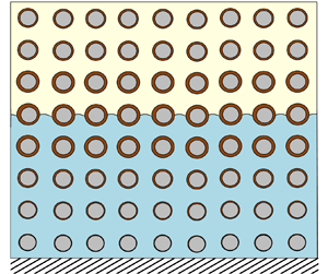
We consider a porous material of finite thickness  $l$, initially with uniform porosity and saturated with a uniform mixture of liquid and suspended dirt. We assume that the dirt particles are small relative to the pore-length scale, and neither interact with each other nor dissolve in the liquid. The dirt–liquid mixture is thus a suspension of these insoluble dirt particles. We suppose the porous material is bounded by an impermeable solid material on one side. The liquid begins to evaporate from the side open to the atmosphere, leaving the dirt behind, and an evaporation front moves into the porous material, with the suspended dirt and liquid ahead of the front, and a mixture of inert gas (drawn in from above the porous material) and liquid vapour behind it. We assume the system is isothermal, with no variation in temperature. A schematic of the situation under consideration is shown in figure 1. We consider a two-dimensional porous material for simplicity, with spatial variables $x$ and $y$, and with $y$ pointing into the porous material and $y=0$ at the surface of the porous material. Although the structure of our model and the homogenisation analysis does not depend on the pore-scale geometry, it is helpful to specify this for simplicity. We choose a square lattice of circular solid inclusions, of radius $r_0$. We account for deposition of the suspended dirt onto the solid structure by considering deposited dirt layers of thickness $R(x,y,t)$, on each solid inclusion, which have initial thickness zero. An important assumption is that the liquid–dirt mixture does not flow, and so our model excludes any capillary pressure or surface tension effects (since in order to attain a (quasi-)static meniscus shape, the liquid would need to flow). We first consider the drying behaviour on the microscale – within the pores of the material – before averaging to derive our effective model. We suppose that the evaporating front is located at $y=h(x,t)$, splitting the domain into a region of pore space containing vapour in $0\leq y\leq h(x,t)$, where the thickness of the layers of deposited dirt do not change with time, and a region of pore space in $h(x,t)\leq y\leq l$ containing the liquid–dirt mixture, where the dirt-layer thicknesses vary in time due to deposition or erosion.

Figure 1. Schematic showing the evaporation front at  $y=h(x,t)$ moving through the pore space (length scale $d$) of a porous material (of depth $l\gg d$), with dirt depositing in a layer of thickness $R(x,y,t)$ on the circular solid inclusions with radius $r_0$. The unit normal to the solid or dirt boundary of the pore space is $\boldsymbol {n}_s$, while the evaporating interface has unit normal $\boldsymbol {m}$.
2.1. Pore-scale model
In the pore space occupied by the vapour–gas mixture (behind the evaporating front, i.e.  $y< h(x,t)$), we expect the Reynolds number to be small (Luckins et al. Reference Luckins, Breward, Griffiths and Please2023) and so we assume that the mixture satisfies the Stokes equations
 \begin{equation} \boldsymbol{\nabla}\boldsymbol{\cdot}\boldsymbol{u}=0, \quad -\boldsymbol{\nabla} p+\mu\nabla^2\boldsymbol{u}=\boldsymbol{0}, \end{equation}
where  $\boldsymbol {u}$ is the mass-averaged velocity of the mixture, $p$ is the pressure and $\mu$ is the viscosity (assumed constant). The vapour contained within the mixture is advected with the flow, and also diffuses through the mixture with diffusivity $D_v$, and thus, the density of the vapour, $\rho _v$ [ ${\rm kg}\ {\rm m}^{-3}$], satisfies
 \begin{equation} (\rho_v)_t+\boldsymbol{u}\boldsymbol{\cdot}\boldsymbol{\nabla}\rho_v=D_v\nabla^2\rho_v, \end{equation}
where the subscript  $t$ denotes partial derivative. The overall density of the inert gas–vapour mixture, $\rho _G$, is given by
 \begin{equation} \rho_G=\rho_g+\rho_v. \end{equation}
Wherever the gas–vapour mixture meets the solid walls of the pore space we suppose there is no flux or slip of the gas–vapour mixture, and no flux vapour into the solid material, so that on the solid–liquid or dirt–liquid boundary, with normal  $\boldsymbol {n}_s$,
 \begin{equation} \boldsymbol{u}=\boldsymbol{0}, \quad \left(\rho_v\boldsymbol{u}-D_v\boldsymbol{\nabla}\rho_v\right)\boldsymbol{\cdot}\boldsymbol{n}_s=0. \end{equation}
 In the liquid–dirt mixture in  $y>h(x,t)$, we assume that there is no net flow of the mixture, and the suspended dirt and liquid diffuse against one another in an ideal mixture, due to Brownian motion. The suspended dirt volume fraction, $\theta$, therefore satisfies
 \begin{equation} \theta_t=D_d\nabla^2\theta, \end{equation}
where  $D_d$ is the diffusivity of suspended dirt in liquid. As discussed in Luckins et al. (Reference Luckins, Breward, Griffiths and Please2023), the assumption that the liquid does not flow means that capillary effects are neglected from the model.
At the solid walls of the pore space, we suppose that the suspended dirt can deposit onto the solid microstructure, forming a layer that may also then be eroded away. We suppose that the deposited layer has a dirt volume fraction  $\theta _*$ which is the packing volume fraction of the dirt particles. We expect this to be close to one, as only a small amount of liquid (volume fraction $1-\theta _*$) is trapped within the deposited dirt layer. Conservation of dirt across the interface is given by
 \begin{equation} \theta V_n +D_d\boldsymbol{\nabla}\theta\boldsymbol{\cdot}\boldsymbol{n}_s = \theta_*V_n, \end{equation}
where  $V_n$ is the normal velocity of the depositing/eroding interface. We note that, in order that there is no flow generated at the depositing interface, we assume that the dirt and liquid have the same mass density, so that the total mixture density is the same on either side of the depositing/eroding interface, while the dirt and liquid fractions can jump (see, for instance, Geng, Kamilova & Luckins Reference Geng, Kamilova and Luckins2023).
We suppose that the dirt is deposited at a rate dependent on the local suspended dirt volume fraction, while the erosion rate depends on the (constant) packing volume fraction  $\theta _*$. (If there was a flow of the fluid, we might extend this model and allow the erosion rate to depend on the local shear stress.) Thus, we prescribe
 \begin{equation} V_n=k_+\theta -k_-\theta_*, \end{equation}
where the constants  $k_\pm$ have units ${\rm m}\ {\rm s}^{-1}$. This type of law-of-mass-action deposition rate, in which the deposition rate is linear in the quantity of suspended dirt, is common in the phenomenological bed-filtration literature (Zamani & Maini Reference Zamani and Maini2009; Dressaire & Sauret Reference Dressaire and Sauret2017), and is also used by Ji & Sanaei (Reference Ji and Sanaei2023) as a model for adsorption of particles onto the deposit layer.
At the evaporating interface  $y=h(x,t)$, we suppose that the inert gas and the dirt do not pass through the interface, while liquid turns into vapour. We thus impose conservation of mass of each of the liquid/vapour, gas, and suspended dirt, namely
 $$\begin{gather} -\rho_l(1-\theta)V_m+\rho_dD_d\boldsymbol{\nabla}\theta\boldsymbol{\cdot}\boldsymbol{m}= \rho_v\left(\boldsymbol{u}\boldsymbol{\cdot}\boldsymbol{m}-V_m\right)-D_v\boldsymbol{\nabla}\rho_v\boldsymbol{\cdot}\boldsymbol{m}, \end{gather}$$
 $$\begin{gather}0=\rho_g\left(\boldsymbol{u}\boldsymbol{\cdot}\boldsymbol{m}-V_m\right)+D_v\boldsymbol{\nabla}\rho_v\boldsymbol{\cdot}\boldsymbol{m}, \end{gather}$$
 $$\begin{gather}-\rho_d\theta V_m-\rho_dD_d\boldsymbol{\nabla}\theta\boldsymbol{\cdot}\boldsymbol{m}=0, \end{gather}$$
where  $\rho _l$ and $\rho _d$ are the densities of pure liquid and dirt, respectively. Combining these, we derive the more helpful form
 $$\begin{gather} -\rho_LV_m=\rho_G\left(\boldsymbol{u}\boldsymbol{\cdot}\boldsymbol{m}-V_m\right), \end{gather}$$
 $$\begin{gather}-\rho_LV_m=\rho_v\left(\boldsymbol{u}\boldsymbol{\cdot}\boldsymbol{m}-V_m\right)-D_v \boldsymbol{\nabla}\rho_v\boldsymbol{\cdot}\boldsymbol{m}, \end{gather}$$
 $$\begin{gather}\theta V_m+D_d\boldsymbol{\nabla}\theta\boldsymbol{\cdot}\boldsymbol{m}=0, \end{gather}$$
interpretable as a condition on each of  $\boldsymbol {u}\boldsymbol {\cdot }\boldsymbol {m}$, $\rho _v$ and $\theta$, respectively, where $\rho _L=\rho _l(1-\theta )+\rho _d\theta$ is the (assumed constant) liquid–dirt mixture density. The normal velocity of the interface and unit normal to the interface are given by
 \begin{equation} V_m=\frac{h_t}{\sqrt{1+h_x^2}}, \quad \boldsymbol{m}=\frac{(h_x,-1)}{\sqrt{1+h_x^2}}, \end{equation}
where subscripts  $t$ and $x$ denote partial derivatives. In addition to (2.9), we also impose a no-slip condition for the gas-mixture velocity
 \begin{equation} u+vh_x=0 \quad \text{on }y=h(x,t). \end{equation}
 Finally, we must also incorporate a condition that describes the chemistry governing the evaporation. In Luckins et al. (Reference Luckins, Breward, Griffiths and Please2023) the effect of different chemistry conditions were considered, and these were shown to affect the form of macroscale boundary conditions derived through a homogenisation analysis. For simplicity, we assume that the liquid and vapour are in chemical equilibrium at the evaporating interface. The chemical potential on the liquid side of the interface is dependent on the amount of liquid ( $1-\theta$) at the interface, while the chemical potential on the gas-mixture side depends on the density of vapour, $\rho _v$, at the interface. In general, we may express this chemical equilibrium as
 \begin{equation} \rho_v=\rho^*f(\theta) \quad \text{on }y=h(x,t), \end{equation}
where  $\rho ^*$ is the (constant) saturation vapour density when $\theta =0$ and there is no suspended dirt, and the function $f(\theta )$ captures the dirt dependence of the saturation vapour density. (We note that therefore $f(0)=1$.) The presence of particles at the interface are expected to hinder the vaporisation; in both Ji & Sanaei (Reference Ji and Sanaei2023) and Karapetsas et al. (Reference Karapetsas, Sahu and Matar2016) the evaporative flux is modelled as decreasing with increased particles on the fluid surface. We keep $f(\theta )$ general as far as possible, and in § 5 we investigate the effect of different functional dependencies $f(\theta )$ on the drying rate. However, in our numerical simulations we use the simple linear form
 \begin{equation} f(\theta)=1-\theta \end{equation}
to capture the effect of the dirt inhibiting vaporisation. We choose this form so that the saturation vapour density scales with the amount of liquid at the interface.
At the surface of the porous material, we impose a constant atmospheric vapour density and atmospheric pressure
 \begin{equation} \rho_v=\rho_a, \quad p=p_a, \quad \text{on }y=0. \end{equation}
Dirt cannot diffuse through the impermeable boundary and thus so impose that
 \begin{equation} \theta_y=0\quad \text{at }y=l. \end{equation}
This depth  $l$ is assumed to be much greater than the typical pore-length scale, so that there is separation between the pore- and macro-length scales.
2.2. Non-dimensionalisation
We non-dimensionalise the vapour/gas problem in a similar way to Luckins et al. (Reference Luckins, Breward, Griffiths and Please2023), making the rescalings
 \begin{align} \boldsymbol{x}=d\hat{\boldsymbol{x}}, \quad h=d\hat{h}, \quad t=\frac{d^2}{\epsilon\delta D_v}\hat{t}, \quad \rho_v=\rho^*\hat{\rho}, \quad \boldsymbol{u}=\frac{D_v\nu\epsilon}{d}\hat{\boldsymbol{u}}, \quad p=p_a+\frac{\mu D_v\nu}{d^2}\hat{p}, \end{align}
where
 \begin{equation} \delta=\frac{\rho^*}{\rho_L}, \quad \epsilon=\frac{d}{l}, \quad \nu=\frac{\rho^*}{\rho_G}\end{equation}
are dimensionless parameters representing the ratio of vapour density to liquid density, the ratio of pore- to macro-length scales and the ratio of vapour to gas densities, respectively. In particular, we note that we have chosen the time scale associated with the speed of the motion of the evaporating interfaces on the microscale, i.e. the time scale over which sufficient vapour is removed by diffusion to empty the microscale pore space of liquid. Making these rescalings and dropping the hat notation, the dimensionless microscale model is, in  $y< h(x,t)$,
 \begin{equation} \epsilon\boldsymbol{\nabla}\boldsymbol{\cdot}\boldsymbol{u}=0, \quad \epsilon\nabla^2\boldsymbol{u}=\boldsymbol{\nabla} p,\quad \epsilon\left(\delta\rho_t+\nu\boldsymbol{u}\boldsymbol{\cdot}\boldsymbol{\nabla}\rho\right)=\nabla^2\rho,\end{equation}
while in  $y>h(x,t)$,
 \begin{equation} \epsilon\sigma\theta_t=\nabla^2\theta.\end{equation}
At gas–solid interfaces in  $y< h(x,t)$ (which are stationary),
 \begin{equation} \boldsymbol{u}=\boldsymbol{0}, \quad \boldsymbol{\nabla}\rho\boldsymbol{\cdot}\boldsymbol{n}_s=0,\end{equation}
and at liquid–solid interfaces in  $y>h(x,t)$ (which move with velocity $V_n$),
 \begin{equation} \boldsymbol{\nabla}\theta\boldsymbol{\cdot}\boldsymbol{n}_s=\epsilon\sigma\left(\theta_*-\theta\right) V_n, \quad V_n=\epsilon\kappa\left(\theta-\beta\right),\end{equation}
while at the evaporating interfaces  $y=h(x,t)$,
 $$\begin{gather} \boldsymbol{u}\boldsymbol{\cdot}\boldsymbol{m}-\delta\nu^{{-}1} \frac{h_t}{\sqrt{1+h_x^2}}={-}\frac{h_t}{\sqrt{1+h_x^2}}, \end{gather}$$
 $$\begin{gather}\epsilon
\rho\Big(\nu\boldsymbol{u}\boldsymbol{\cdot}\boldsymbol{m}-\delta
\frac{h_t}{\sqrt{1+h_x^2}}\Big)-\boldsymbol{\nabla}\rho\boldsymbol{\cdot}
\boldsymbol{m}={-}\epsilon\frac{h_t}{\sqrt{1+h_x^2}},
\end{gather}$$
$$\begin{gather}\epsilon
\rho\Big(\nu\boldsymbol{u}\boldsymbol{\cdot}\boldsymbol{m}-\delta
\frac{h_t}{\sqrt{1+h_x^2}}\Big)-\boldsymbol{\nabla}\rho\boldsymbol{\cdot}
\boldsymbol{m}={-}\epsilon\frac{h_t}{\sqrt{1+h_x^2}},
\end{gather}$$ $$\begin{gather}u+vh_x=0, \end{gather}$$
 $$\begin{gather}\epsilon\sigma\theta V_m+ \boldsymbol{\nabla}\theta\boldsymbol{\cdot}\boldsymbol{m}=0, \end{gather}$$
 $$\begin{gather}\rho=f(\theta). \end{gather}$$
At the surface of the porous material,
 \begin{equation} \rho=\alpha \quad \text{at }y=0,\end{equation}
while at the impermeable surface (or centre of a symmetric porous material),
 \begin{equation} \theta_y=0 \quad \text{at }y=\epsilon^{{-}1}.\end{equation}
Here we have introduced the additional dimensionless parameters
 \begin{equation} \sigma=\delta\frac{D_v}{D_d}, \quad \kappa=\frac{k_+d}{\epsilon^2\delta D_v}, \quad \beta=\frac{k_-\theta_*}{k_+}, \quad \alpha=\frac{\rho_a}{\rho^*} \end{equation}
that appear in the dirt problem, representing the ratio of the suspended dirt diffusion time scale to the time scale of the evaporation-front motion, the ratio of the dirt-deposition rate to the evaporation rate, the ratio of the dirt erosion rate to deposition rate and the ratio of the atmospheric vapour density to the maximum saturation vapour density, respectively.
The micro- to macro-length scale ratio  $\epsilon$ (defined in (2.17a–f)) is the small parameter we take advantage of in order to homogenise (2.18). As in Luckins et al. (Reference Luckins, Breward, Griffiths and Please2023), we take $\delta <1$ and $\nu <1$ to be order one parameters relative to $\epsilon$ for the homogenisation analysis. We note that $\delta \approx 10^{-3}$ for water, so will later consider the additional limit of $\delta \rightarrow 0$ (which is equivalent to taking this limit before performing the homogenisation analysis). We require $\alpha <1$ but expect $\alpha \ll 1$ to be reasonable. Although the diffusion of vapour in air is generally much faster than the diffusion of any kind of molecule through a liquid, so that $D_v\gg D_d$, we note that since $\delta \approx 10^{-3}\unicode{x2013}10^{-4}$ is small, $\sigma$ is likely to be order one. For instance, if we take $D_v\approx 2.5\times 10^{-5}\ {\rm m}^2\ {\rm s}^{-1}$ and $D_d\approx 10^{-9}\ {\rm m}^2\ {\rm s}^{-1}$ (Cussler Reference Cussler2009), then with $\delta =10^{-4}$ we find that $\sigma \approx 2.5$. We consider the distinguished limit of $\sigma =O(1)$ in this paper, but we note there is an alternative, slow-dirt-diffusion, distinguished limit with $\sigma =O(\epsilon ^{-1})$. We discuss this alternative case further in Appendix A.2, and briefly in § 2.3 below. In summary, all of $\sigma, \kappa, \beta$ and $\alpha$ are taken to be order one relative to $\epsilon$ to homogenise the model.
2.3. Summary of the homogenised drying model
The homogenisation analysis is described in Appendix A. The result of this analysis is a macroscale model for the vapour density  $\rho$, suspended dirt volume fraction $\theta$, deposited dirt-layer thickness, $R$, and position, $Y=H(T)$ of the evaporation front, namely
 \begin{equation} \delta\phi\rho_T-(\nu-\delta)\phi|_H H_T\rho_Y= \left(\mathcal{D}\rho_Y\right)_Y\end{equation}
for  $Y< H(T)$, and
 $$\begin{gather} \sigma\phi\theta_T=(\mathcal{D}\theta_Y)_Y-\sigma\kappa\mathcal{C}(\theta_*-\theta)(\theta-\beta\chi_R), \end{gather}$$
 $$\begin{gather}R_T=\kappa(\theta-\beta\chi_R) \end{gather}$$
for  $Y>H(T)$. At $Y=H(T)$,
 $$\begin{gather} \mathcal{D}\rho_Y=(1-\nu\rho)\phi H_T, \end{gather}$$
 $$\begin{gather}\rho=f(\theta), \end{gather}$$
 $$\begin{gather}\sigma\phi H_T\theta+\mathcal{D}\theta_Y=0, \end{gather}$$
while
 $$\begin{gather} \rho=\alpha \quad\text{on }Y=0, \end{gather}$$
 $$\begin{gather}\theta_Y=0 \quad\text{on }Y=1. \end{gather}$$
The porosity,  $\phi (R)=1-{\rm \pi} (r_0+R)^2$, surface area, $\mathcal {C}(R)=2{\rm \pi} (r_0+R)$, and effective diffusivity, $\mathcal {D}(R)$ (given by (A4)), all vary with the thickness of the deposited dirt layer.
We assume that, initially, the porous material is entirely saturated with a uniform liquid–dirt mixture, none of which has yet deposited (i.e. the time scale of deposition is assumed longer than the time scale over which the liquid–dirt mixture flooded the material). Thus, at  $T=0$,
 \begin{equation} R=0, \quad H=0, \quad \theta=\theta_{IC}.\end{equation}
 Our homogenised model (2.20) is similar in structure to those proposed in Breward et al. (Reference Breward2020), Sanaei et al. (Reference Sanaei2022) and Ji & Sanaei (Reference Ji and Sanaei2023), with the suspended dirt satisfying a reaction–diffusion equation ahead of a moving evaporation front. However, through the systematic homogenisation analysis, we have found the correct form for the diffusion term in (2.20b), which was erroneously given as  $(D(\phi \theta )_Y)_Y$ (in our notation) by Ji & Sanaei (Reference Ji and Sanaei2023). Additionally, we have quantified the effective parameters $\mathcal {D}$, $\mathcal {C}$ and $\phi$, which all vary with the deposited dirt-layer thickness $R$. We also impose different boundary conditions to Ji & Sanaei (Reference Ji and Sanaei2023), which will result in different drying behaviours, as discussed in § 3 below.
A key assumption of our homogenisation analysis was that  $\sigma =O(1)$, which ensured that $\theta$ (and therefore $R$) is uniform to leading order on the microscale. As discussed further in Appendix A.2, the extremely slow suspended dirt diffusion limit of $\sigma =O(\epsilon ^{-1})$ is not captured by this model: in this case we would expect non-periodic behaviour on the microscale at the evaporating interface, and the homogenisation analysis would break down. We do not consider this situation here.
3. An ODE for the motion of the evaporation front
The parameter  $\delta =\rho ^*/\rho _L$ is generally small; indeed for water evaporating we expect $\delta \approx 10^{-3}$. Before studying the full drying problem, we consider the limit of $\delta \rightarrow 0$ in the vapour–gas transport problem, which we show results in a single ODE describing the motion of the evaporation front $H(T)$. This gives insight into the drying dynamics and is interesting as a comparison with other models for the motion of evaporating interfaces in the literature, e.g. Ji & Sanaei (Reference Ji and Sanaei2023). Furthermore, the analysis in this section is helpful for all of the subsequent analysis of the model, including the early time asymptotic analysis in the following section (§ 4), which we use to initialise numerical simulations of the model.
For small  $\delta$, we see from (2.20a) that the vapour-density profile is quasi-steady, varying instantaneously with the motion of the evaporation front. Specifically, in the limit $\delta \rightarrow 0$, the vapour-transport equation (2.20a) becomes
 \begin{equation} -\nu\phi|_H H_T\rho_Y=( \mathcal{D}\rho_Y )_Y. \end{equation}
Integrating twice with respect to  $Y$ and applying the boundary conditions (2.20d) and (2.20g), we obtain
 \begin{equation} \rho=\frac{1}{\nu}\left(1-(1-\nu \alpha)\exp\left(-\nu \phi|_H H_T\int_0^Y \frac{1}{\mathcal{D}(R(\hat{Y}))}\,\mathrm{d}\hat{Y}\right)\right). \end{equation}
By additionally imposing the boundary condition (2.20e) we obtain an equation for the motion of the evaporation front,  $H$, in terms of the suspended dirt volume fraction there, $\theta |_{H}$, namely
 \begin{equation} H_T\int_0^H \frac{1}{\mathcal{D}(R(\hat{Y}))}\,\mathrm{d}\hat{Y}=\frac{1}{\nu \phi|_H}\log\left(\frac{1-\nu \alpha}{1-\nu f(\theta|_{H})}\right).\end{equation}
One particular case of interest is if  $\mathcal {D}$ is uniform (for instance, if little dirt has been deposited, so $R\approx 0$ is constant). In this case (3.3) reduces to
 \begin{equation} HH_T=\frac{\mathcal{D}}{\nu\phi|_H}\log\left(\frac{1-\nu \alpha}{1-\nu f(\theta|_H)}\right).\end{equation}
If  $\theta |_H$ were constant, we would see a $\sqrt {T}$ behaviour of the evaporation front, as expected for this type of Stefan problem. For $\mathcal {D}$ non-uniform in $Y$, the integral term in (3.3) behaves like an overall resistance to vapour transport. In particular, the integral is dominated by any localised regions of pore space in $Y< H$ for which $\mathcal {D}$ is very small.
We see that the ODE (3.4) for  $H$ (with $\mathcal {D}$ constant) takes the form
 \begin{equation} HH_T=E_1(\phi|_H,\theta|_H)\end{equation}
for an algebraic function  $E_1$, while the more general (3.3) takes the form
 \begin{equation} H_T=E_2(\phi|_H,\theta|_H,H,R|_{Y< H}).\end{equation}
By comparison, Ji & Sanaei (Reference Ji and Sanaei2023) prescribe an evaporative flux that does not explicitly depend on  $H$, of the form
 \begin{equation} H_T=E_3(\phi|_H,\theta|_H),\end{equation}
in our notation. Unlike (3.5) and (3.6), the model (3.7) does not explicitly depend on the position  $H$ of the evaporating interface. These different equations for $H$ result from different modelling assumptions: Ji & Sanaei (Reference Ji and Sanaei2023) assume that the vaporisation of the liquid molecules is the limiting process in the evaporation, whereas we have assumed that the vaporisation is instantaneous (the vapour is at its saturation point adjacent to $Y=H$) and that evaporation is instead limited by the transport of vapour out of the porous material. For sufficiently deep or hydrophobic porous media that there is a moving drying front, it is clear that the evaporation rate should depend on the location $H$ of the drying front (Lehmann et al. Reference Lehmann, Assouline and Or2008; Shokri et al. Reference Shokri, Lehmann and Or2008). Furthermore, we note that our drying model is given in terms of well-defined physical parameters such as the diffusivity and saturation vapour densities, and results in a reasonable drying time scale $l^2\rho _L/\rho _* D_v\approx 10^{2}$ s (using values for water: $\rho _L\approx 10^3\ {\rm kg}\ {\rm m}^{-3}$, $\rho _*\approx 1\ {\rm kg}\ {\rm m}^{-3}$, $D_v\approx 10^{-5}\ {\rm m}^2\ {\rm s}^{-1}$ and $l\sim 10^{-3}\ {\rm m}$), whereas the coefficients in a prescribed evaporation rate must be fitted in some way.
We note from (3.3) that evaporation only occurs when  $f(\theta |_H)>\alpha$, so that the vapour density at the liquid–gas interface is greater than the atmospheric vapour density; otherwise if $f(\theta |_H)=\alpha$, we see that $H_T=0$. We define $\hat {\theta }$ such that $f(\hat {\theta })=\alpha$, noting that since $f$ is monotonic in $\theta$, evaporation only occurs for $\theta <\hat {\theta }$.
Our analysis above (and in the remainder of this paper) is for the case that the atmospheric vapour density  $\rho =\alpha$ is prescribed at the surface $Y=0$. As an aside, we now briefly consider an alternative case, in which the flux, $J$, of vapour out of the material at $Y=0$ is prescribed by a Newton cooling law: $J=m(\rho |_0-a_\infty )$, for some constants $a_\infty$ (the far-field ambient vapour density) and $m$ (the mass-transfer coefficient). Since the vapour flux is spatially uniform throughout $Y< H$ in the limit $\delta \ll 1$, we find that $\phi |_H H_T=m(\rho |_0-a_\infty )$. Eliminating $\rho |_0$, we find that $H_T$ is given by the implicit ODE
 \begin{equation} H_T\int_{Y=0}^H\frac{1}{\mathcal{D}}\,\mathrm{d}Y=\frac{1}{\nu\phi|_H}\log\left(\frac{1-\nu a_\infty-\nu\phi|_HH_T/m}{1-\nu f(\theta|_H)}\right).\end{equation}
(We may rearrange (3.8) to give  $H_T$ explicitly in terms of a Lambert- $W$ function, but we consider the form (3.8) more useful as we may compare directly with (3.3).) Clearly in the limit as $m\rightarrow \infty$ (for which vapour is easily removed from the surface of the porous material), and with $a_\infty =\alpha$ we regain (3.3). In the case of a bounded mass-transfer coefficient $m$, the non-instantaneous removal of vapour from the surface results in a slower evaporation rate $H_T$, compared with that given by (3.3).
4. Early time behaviour and numerical method
In this section we first consider the early time behaviour of our model (2.20) in § 4.1, in the limit of  $\delta \ll 1$. This will be necessary in order to accurately initialise numerical simulations of the model, which is then discussed in § 4.2.
4.1. Early time analysis
To study the early time behaviour of the system (2.20), we suppose  $T=b\tau$ where $b\ll 1$ is the smallest parameter in the system, and $\tau =O(1)$. From (2.20c), on this time scale we see that $R_\tau =O(b\kappa )\ll 1$, and so $R$ is small, hence, all of $\mathcal {D},\phi$ and $\mathcal {C}$ are constant to leading order in $b$.
$b$.
We first consider the vapour problem in  $Y< H$. On the short time scale the interface only moves a short distance, and so we rescale
 \begin{equation} H=\sqrt{\frac{b\mathcal{D}}{\phi}}\bar{H}, \quad Y=\sqrt{\frac{b\mathcal{D}}{\phi}}\bar{Y} \end{equation}
in order to balance the mass-flux boundary condition (2.20d). The vapour problem is therefore self-similar in that we regain the same system at early time with these rescalings as the full system (2.20a), (2.20d)–(2.20e) and (2.20g), namely
 $$\begin{gather} \delta\rho_\tau-(\nu-\delta) \bar{H}_\tau\rho_{\bar{Y}}=\rho_{\bar{Y}\bar{Y}}, \quad\text{for } \bar{Y}\in(0,\bar{H}(\tau)), \end{gather}$$
 $$\begin{gather}\rho=\alpha \quad\text{on }\bar{Y}=0, \end{gather}$$
 $$\begin{gather}\rho_{\bar{Y}}=(1-\nu\rho) \bar{H}_\tau \quad\text{on }\bar{Y}=\bar{H}(\tau), \end{gather}$$
 $$\begin{gather}\rho=f(\theta) \quad\text{on }\bar{Y}=\bar{H}(\tau). \end{gather}$$
We have already noted that  $\delta \ll 1$ in general, and we take this limit now to make analytical progress. As in § 3, we find that
 \begin{equation} \rho=\frac{1}{\nu}\left(1-(1-\nu \alpha)\exp\left(-\nu \bar{H}_\tau \bar{Y}\right)\right),\end{equation}
where  $\bar {H}(\tau )$ is the solution of
 \begin{equation} \bar{H}\bar{H}_\tau=\frac{1}{\nu}\log\Big(\frac{1-\nu \alpha}{1-\nu f(\theta|_{\bar{Y}=\bar{H}(\tau)})}\Big).\end{equation}
 The value of  $\theta$ at $\bar {Y}=\bar {H}(\tau )$ depends on the solution of the suspended dirt problem in the domain $Y\in (H,1)=(\sqrt {b\mathcal {D}/\phi }\, \bar {H}(\tau ),1)$. On this short time scale, the full dirt problem (2.20b), (2.20f) and (2.20h), with the initial condition (2.21a–c), becomes
 $$\begin{gather} \sigma\phi\theta_\tau=b\left(\mathcal{D}\theta_{YY}-\sigma\kappa\mathcal{C}(\theta_*-\theta)(\theta-\beta\chi_R)\right) \quad\text{for }Y\in(\sqrt{b\mathcal{D}/\phi}\, \bar{H}(\tau),1), \end{gather}$$
 $$\begin{gather}\sigma \phi\theta \bar{H}_\tau+\sqrt{b}\mathcal{D}\theta_Y=0 \quad\text{on }Y=\sqrt{b\mathcal{D}/\phi}\, \bar{H}(\tau), \end{gather}$$
 $$\begin{gather}\theta_Y=0 \quad\text{on }Y=1, \end{gather}$$
 $$\begin{gather}\theta=\theta_{IC} \quad\text{at }\tau=0. \end{gather}$$
To leading order in  $b$, we see that $\theta _\tau =0$, so that $\theta =\theta _{IC}$ is independent of time over the domain. However, in a boundary layer at $Y=\sqrt {b\mathcal {D}/\phi } \bar {H}$, suspended dirt accumulates due to the motion of the evaporation front. To examine this region, we make the change of variables $Y=\sqrt {b\mathcal {D}/\phi }(\bar {H}(\tau )+z)$, so that, at leading order in $b$, the equations are
 $$\begin{gather} \sigma\left(\theta_\tau-\bar{H}_\tau\theta_z\right)=\theta_{zz} \quad\text{for }z>0, \end{gather}$$
 $$\begin{gather}\sigma\theta \bar{H}_\tau+\theta_z=0 \quad\text{on }z=0, \end{gather}$$
 $$\begin{gather}\theta\rightarrow\theta_{IC} \quad\text{as }z\rightarrow\infty, \end{gather}$$
 $$\begin{gather}\theta=\theta_{IC} \quad\text{at }\tau=0. \end{gather}$$
This system (4.6) must be solved with (4.4) to determine  $\theta$ and $\bar {H}$.
We look for a similarity solution of the form
 \begin{equation} \bar{H}=\frac{2\lambda}{\sqrt{\sigma}}{\sqrt{\tau}}, \quad \theta=\varTheta\left(\frac{\sqrt{\sigma}z}{\sqrt{ \tau}}\right),\end{equation}
for some constant  $\lambda$ to be determined. In particular, from (4.4) we see that the suspended dirt volume fraction at the evaporating interface, $\theta |_{\bar {H}}=\varTheta (0)$, must be constant in time for such a similarity solution to exist. Substituting into (4.6), we find the solution
 \begin{equation} \varTheta=\theta_{IC}+\left(\varTheta(0)-\theta_{IC}\right)\frac{\text{erfc}\left(\lambda+ \dfrac{\sqrt{\sigma}z}{2\sqrt{ \tau}}\right)}{\text{erfc}(\lambda)} ,\end{equation}
where  $\lambda$ and the constant $\varTheta (0)$ satisfy
 $$\begin{gather} \lambda^2=\frac{\sigma}{2\nu}\log\left(\frac{1-\nu \alpha}{1-\nu f(\varTheta(0))}\right), \end{gather}$$
 $$\begin{gather}\varTheta(0)=\theta_{IC}+\sqrt{\rm \pi}\lambda\varTheta(0){\rm e}^{\lambda^2}\,\text{erfc}(\lambda). \end{gather}$$
Solutions of (4.9)–(4.10) may be computed numerically, and are shown for various  $\sigma$ and $\theta _{IC}$ in figure 2.

Figure 2. Early time solution behaviour. Coloured lines show the variation of the solution of (4.9) and (4.10) with the suspended dirt diffusion time scale  $\sigma$. Green dashed lines are the small- $\sigma$ approximations (4.11), while black dashed lines are the large- $\sigma$ approximations (4.13). Here we use the form $f(\theta )=1-\theta$ and set $\alpha =0$, so that $\hat {\theta }=1$. We additionally set $\nu =0.5$.
To establish some intuitive understanding of this early time behaviour, we now consider the sublimits  $\sigma \ll 1$, $\theta _{IC}\ll 1$ and $\sigma \gg 1$ in turn. We show our early time analytic solutions for each case in figure 3 (alongside numerical solutions for comparison, computed using the method described in § 4.2 below), all with excellent agreement. In each, we see that the vapour density $\rho$ varies from $f(\theta |_H)=1-\theta |_H$ at $Y=H$ to $\alpha =0$ at the surface of the material, according to (4.3). The evaporation front moves with the expected $\sqrt {T}$ behaviour, faster if there is a steeper vapour-density gradient. Suspended dirt accumulates in the liquid ahead of the evaporation front, with a spatial maximum in $\theta$ at $Y=H$. The size of the boundary layer at $H$ over which $\theta$ varies is dependent on $\sigma$, which quantifies suspended dirt diffusion. At early times, we expect little dirt deposition, so that the dirt-layer thickness $R\approx 0$ throughout the porous material.

Figure 3. Early time solutions (4.3), (4.7a,b) and (4.8) (dotted lines) compared with numerical solutions (solid lines) of the full model (2.20), for  $\sigma =0.01$ (a,b) $\sigma =1$, (c,d) and $\sigma =10$ (e,f). The profiles of $\rho$, $\theta$ and $R$ in figures a, c, and e are at times for which $H=0.3$ (towards the end of what we would consider ‘early’ time, especially in the small- $\sigma$ case). Throughout the figure we take $f(\theta )=1-\theta$, $\kappa =1$, $\theta _{IC}=0.1$, $\nu =0.5$, $\delta =10^{-3}$, $r_0=0.2$, $\alpha =0$ and $\beta =0$.
If  $\sigma \ll 1$ so that suspended dirt diffusion is fast relative to the motion of the evaporation front, then we see from (4.9) that $\lambda =O(\sqrt {\sigma })$, and so from (4.10) that $\theta |_h\sim \theta _{IC}$. Specifically, we find that
 \begin{equation} \left.\begin{array}{c} \varTheta(0)=\theta_{IC}+O(\sqrt{\sigma}),\\[3pt] \lambda=\sqrt{\sigma}\left(\sqrt{\dfrac{1}{2\nu}\log\left(\dfrac{1-\nu \alpha}{1-\nu f(\theta_{IC})}\right)}+O (\sqrt{\sigma})\right)\end{array}\!\!\right\} \quad \text{as }\sigma\rightarrow 0.\end{equation}
Thus, reverting to our original variables, the early time evaporating interface is given by
 \begin{equation} H=\sqrt{T}\sqrt{\frac{\mathcal{D}}{2\nu\phi}\log\left(\frac{1-\nu \alpha}{1-\nu f(\theta_{IC})}\right)}+O(\sqrt{\sigma}) \quad \text{as }\sigma\rightarrow 0. \end{equation}
We also note from the form (4.8) of the solution that the spatial region over which  $\theta$ varies is wide, $O(1/\sqrt {\sigma })$. In this small- $\sigma$ limit, the diffusion of dirt is fast relative to the motion of the evaporation front, and so the suspended dirt volume fraction $\theta$ remains close to its initial value $\theta _{IC}$, only deviating by a small, $O(\sqrt {\sigma })$, amount. For conservation of overall dirt, the region over which the accumulating suspended dirt is spread is wide, of $O(1/\sqrt {\sigma })$ relative to the early time boundary layer. This may be seen in figure 3(a,b): since $\sigma \ll 1$, the $\theta$ profile is approximately uniform in $Y$, and so close to its initial value of $\theta _{IC}=0.1$ at early times. The suspended dirt is accumulating due to the evaporation, but spread almost evenly through the domain.
Next, we suppose that  $\sigma =O(1)$ but the initial suspended dirt volume fraction $\theta _{IC}\ll 1$ is small. In this case, for a balance in both of (4.9) and (4.10), we must have $\varTheta (0)=O(\theta _{IC})$ and $\lambda =O(1)$, as we might expect. The solution shown in figure 3(c,d) is for this case, with $\theta _{IC}=0.1$: we indeed observe that $\theta |_H=O(0.1)$ (and this effect becomes increasingly clear for smaller $\theta _{IC}$).
Finally, if  $\sigma \gg 1$, so that the diffusion of suspended dirt is slow relative to the motion of the evaporation front, then from (4.9) we see that we must have $f(\varTheta (0))=\alpha$ to leading order in $\sigma ^{-1}\ll 1$. At this value,
 \begin{equation} \varTheta(0)=\hat{\theta}, \end{equation}
there is no evaporation at leading order, as the vapour density at the atmospheric value is in equilibrium with the liquid–dirt interface, and there is no transport of vapour out of the porous material. Indeed, we see from (4.10) that when  $\theta =\hat {\theta }$, $\lambda$ is the solution of
 \begin{equation} \lambda {\rm e}^{\lambda^2}\,\text{erfc}(\lambda)=\frac{\hat{\theta}-\theta_{IC}}{\hat{\theta}\sqrt{\rm \pi}}, \end{equation}
which is independent of  $\sigma$ and of $O(1)$, so that the position of the evaporating interface, given by
 \begin{equation} H=\frac{2\lambda}{\sqrt{\sigma}}\sqrt{\frac{\mathcal{D}}{\phi}}\sqrt{T}, \end{equation}
is of order  $\sigma ^{-1/2}\ll 1$ away from its initial position. Thus, when the suspended dirt diffusion is slow, the diffusion of dirt away from $H$ limits the speed of the evaporation front, so that there is a slower, $O(\sigma )$, drying time scale. We also note from (4.8) that the region over which $\theta$ varies is narrow, with width $O(1/\sqrt {\sigma })$ relative to the early time boundary layer. The boundary layer is narrow for large $\sigma$, so that the early time solution actually remains valid for the majority of the drying process. Indeed, in figure 3(e,f) we see excellent agreement between the early time analytic solution and the numerical solution for $\rho, \theta$ and $H$ up to the time when the evaporating front is halfway through the domain. This is because the boundary layer at $H$ over which $\theta$ varies is narrow, and so the effect of the boundary at $Y=1$ is not felt until $H$ is close to 1. However, we notice in figure 3(e) that the early time approximation $R=0$ ceases to be accurate at these late times. The early time solution would remain valid so long as $R$ remains relatively small (e.g. if $\kappa$ and $\theta _{IC}$ are fairly small). We note that, since the boundary layer width scales with $\sqrt {T}$, it quickly becomes numerically impractical to resolve the solution at small times for large $\sigma$. The early time asymptotic solution is therefore very valuable in initialising the simulations accurately for large $\sigma$.
Finally, we note that our early time analysis in this section is equivalent to studying the original problem on a semi-infinite domain  $Y\in (0,\infty )$, in the combined limit $\kappa,\delta \rightarrow 0$.
4.2. Numerical method
We solve the model (2.20) numerically using the method of lines. Specifically, we first transform the model onto two separate fixed domains, setting  $\eta =Y/H(T)$ for the gas–vapour problem, which then holds in $\eta \in (0,1)$, and setting $\xi =(Y-H(T))/(1-H(T))$ for the liquid–dirt problem, which then also holds in $\xi \in (0,1)$. We discretise spatially on these transformed domains, with a uniform mesh, using central differences for diffusive terms and first-order upwinding for advective terms, so that the scheme is overall first order. (The advection for the vapour problem (2.20a), including the artificial advection terms due to the change of variables, is negative; the purely artificial advection in the liquid–dirt problem (2.20b)–(2.20c) is also negative. Upwinding these terms therefore requires forward differences in both cases.) We then use the inbuilt ODE solver ode15s in Matlab for the time stepping. We note that the model is stiff in certain parameter regimes of interest ( $\delta \ll 1$ and/or $\sigma \ll 1$), and that ode15s is specifically designed for stiff systems. Ode15s is a multistep solver, using numerical differentiation formulas of order 1–5 (Shampine & Reichelt Reference Shampine and Reichelt1997). We make use of our early time asymptotic solution of § 4.1 to initialise our numerical simulations. In particular, the spatial mesh must be sufficiently fine to resolve the boundary layer in the suspended dirt problem at $Y=H$ at early times. Our analysis in § 4.1 suggests we require the number of spatial mesh points $N$ to scale like
 \begin{equation} N=O\left(\sqrt{\frac{\mathcal{D}(0)\sigma}{\phi(0)T}}\right) \quad \text{for }T\ll1. \end{equation}
More efficient solvers might take further advantage of the asymptotic structure of the system and distribute mesh points unevenly through the domain in order to ensure good resolution of the boundary layer while maintaining computational efficiency. However, by making use of our early time asymptotic solution we do not require simulations at particularly small  $T$, and our uniform-mesh formulation suffices.
5. The slow deposition limit  $\kappa \ll 1$ and dry clogging

Having stated the model and our numerical solution method, we are now in a position to explore solutions of the model. In this section we focus on the limit  $\kappa \ll 1$, for which the dirt-deposition time scale is much longer than the evaporation time scale. We expect that the accumulation of suspended dirt due to evaporation and the effects of suspended dirt diffusion to be dominant.
We first consider the leading-order behaviour, taking  $\kappa =0$, and show that the evaporation becomes infinitely slow as suspended dirt accumulates. We then allow $\kappa$ to be small but non-zero, and explore our first clogging scenario, which we term ‘dry clogging’.
5.1. Infinitely slow evaporation when $\kappa =0$

Taking  $\kappa =0$, we see from (2.20c) that we have $R=0$ everywhere, and thus, $\mathcal {D}=\mathcal {D}_0$, $\mathcal {C}=\mathcal {C}_0$ and $\phi =\phi _0$ are all constant, equal to their values at $R=0$. Taking the $\delta \ll 1$ limit as in § 3, the motion of the evaporation front is therefore governed by (3.4), i.e.
 \begin{equation} HH_T={-}\frac{\mathcal{D}_0}{\nu\phi_0}\log\left(\frac{1-\nu f(\theta|_H)}{1-\nu \alpha}\right),\end{equation}
while  $\theta$ satisfies
 $$\begin{gather} \frac{\sigma\phi_0}{\mathcal{D}_0}\theta_T=\theta_{YY} \quad\text{for }Y\in(H(T),1), \end{gather}$$
 $$\begin{gather}\frac{\sigma\phi_0}{\mathcal{D}_0}\theta H_T+\theta_Y=0 \quad\text{on }Y=H(T), \end{gather}$$
 $$\begin{gather}\theta_Y=0 \quad\text{on }Y=1, \end{gather}$$
 $$\begin{gather}\theta=\theta_{IC} \quad\text{at }T=0. \end{gather}$$
 To investigate how the accumulation of suspended dirt affects the evaporation rate, we consider the additional limit of  $\sigma \ll 1$ so that the diffusion of suspended dirt is fast. In this case, we see from (5.2) that $\theta (T)$ is uniform, and so, for overall conservation of dirt, we must have
 \begin{equation} \theta(T)=\frac{\theta_{IC}}{1-H(T)}.\end{equation}
Substituting (5.3) into (5.1) we obtain the single equation for  $H(T)$,
 \begin{equation} HH_T={-}\frac{\mathcal{D}_0}{\nu\phi_0}\left[\log\left(1-\nu f\left(\frac{\theta_{IC}}{1-H}\right)\right)-\log(1-\nu \alpha)\right].\end{equation}
As discussed previously, the evaporation shuts down when  $\theta =\hat {\theta }$ so that $f(\hat {\theta })=\alpha$, since then $H_T=0$. At this point we see from (5.3) that $H=1-\theta _{IC}/\hat {\theta }$.
Numerical solutions of the model (2.20) (with  $\kappa =0$, $\delta =10^{-3}$) are shown in figures 4(a) and 4(b), and compared with the solution of (5.4) for the limit of $\sigma \rightarrow 0$, with good agreement for $\sigma =0.1$ and smaller. We take the functional form $f(\theta )=1-\theta$ for these simulations, and fix $\alpha =0$ (so that $\hat {\theta }=1$). In figure 4(c) we show solutions of (5.4) for various $\theta _{IC}$. We see that, for larger $\theta _{IC}$, the evaporation is slower, with the evaporating interface $H$ moving more slowly into the domain. In particular, we note that when $\theta _{IC}=0$, the evaporation is completed (with $H=1$) in finite time
 \begin{equation} T={-}\frac{\nu\phi_0}{2\mathcal{D}_0\log(1-\nu)}\approx 0.36, \end{equation}
(from (5.4) with  $\theta _{IC}=0$), whereas for $\theta _{IC}>0$, we see that $H$ appears to take infinite time to reach $1-\theta _{IC}/\hat {\theta }$.

Figure 4. The effect of suspended dirt accumulation on the evaporation, for  $\kappa =0$ and $\sigma \ll 1$. Numerical solutions of (2.20) shown with $\kappa =0$ (no dirt deposition), alongside the solution of (5.4) in the limit $\sigma \rightarrow 0$, (taking $f(\theta )=1-\theta$ and $\alpha =0$). Throughout the figure we take $\nu =0.5$ and $r_0=0.2$. (a) Motion of the evaporation front $H(T)$ for various $\sigma$, with $\theta _{IC}=0.3$. (b) Vapour density and suspended dirt volume fraction profiles at the same time $T=0.2$ for various $\sigma$, with $\theta _{IC}=0.3$. (c) Effect of $\theta _{IC}$ on the evaporating interface motion. Dashed lines are $1-\theta _{IC}$.
We investigate this late time behaviour (within the  $\sigma \ll 1$ limit) by considering the expansion
 \begin{equation} H=1-\frac{\theta_{IC}}{\hat{\theta}}(1+c\mathcal{H}) \quad \text{so that}\ \theta=\frac{\hat{\theta}}{1+c\mathcal{H}},\end{equation}
where  $c\ll 1$ is small and $\mathcal {H}=O(1)$ is positive. Assuming that $f$ is continuous at $\theta =\hat {\theta }$, on substitution of (5.6) into (5.4) we find that (retaining only leading-order terms on either side)
 \begin{align}
c\left(1-\frac{\theta_{IC}}{\hat{\theta}}\right)\frac{\theta_{IC}}{\hat{\theta}}\mathcal{H}_T&={-}
\frac{\mathcal{D}_0}{\phi_0(1-\nu
\alpha)}\biggl(f\biggl(\frac{\hat{\theta}}{1+c\mathcal{H}}\biggr)-\alpha\biggr)\nonumber\\
&={-}\frac{\mathcal{D}_0}{\phi_0(1-\nu \alpha)}(
f(\hat{\theta}(1-c\mathcal{H}+O(c^2)))-\alpha).
\end{align}
\begin{align}
c\left(1-\frac{\theta_{IC}}{\hat{\theta}}\right)\frac{\theta_{IC}}{\hat{\theta}}\mathcal{H}_T&={-}
\frac{\mathcal{D}_0}{\phi_0(1-\nu
\alpha)}\biggl(f\biggl(\frac{\hat{\theta}}{1+c\mathcal{H}}\biggr)-\alpha\biggr)\nonumber\\
&={-}\frac{\mathcal{D}_0}{\phi_0(1-\nu \alpha)}(
f(\hat{\theta}(1-c\mathcal{H}+O(c^2)))-\alpha).
\end{align}
So long as the gradient of the function  $f$ is bounded at $\hat {\theta }$, we may Taylor expand the right-hand side of (5.7) and, thus, find that, to leading order in $c$,
$c$,
 \begin{equation} \mathcal{H}_T=\frac{\mathcal{D}_0\hat{\theta}^3}{\phi_0(1-\nu \alpha)\theta_{IC}(\hat{\theta}-\theta_{IC})}f'(\hat{\theta})\mathcal{H}, \end{equation}
since  $f(\hat {\theta })=\alpha$ by definition. Thus, $\mathcal {H}$ decays exponentially to zero as $T\rightarrow \infty$ (since $f'(\hat {\theta })<0$) and the evaporation takes infinite time. (Similarly, if $f'(\hat {\theta })=0$ but higher derivatives are non-zero then $\mathcal {H}$ has polynomial, and still infinite-time, decay.)
We might ask if there are sensible choices for  $f(\theta )$ that result in finite-time completion of the evaporation. In order for the evaporation to complete in finite time, we see that the gradient of $f$ must be unbounded at $\hat {\theta }$. For instance, if $f(\hat {\theta }(1-c\mathcal {H}))=\alpha +A(c\mathcal {H})^{1/n}$, for $n> 1$ and some constant $A$, then by substituting this expansion for $f$ into (5.7) and integrating the resulting ODE for $\mathcal {H}$ in time $T$, we find that
 \begin{equation}
\mathcal{H}\sim\Big(\text{const.}-\frac{D_0\hat{\theta}^2A(n-1)}{\phi_0\theta_{IC}(\hat{\theta}-\theta_{IC})(1-\nu
\alpha) n}c^{-(n-1)/n}T\Big)^{n/(n-1)},
\end{equation}
\begin{equation}
\mathcal{H}\sim\Big(\text{const.}-\frac{D_0\hat{\theta}^2A(n-1)}{\phi_0\theta_{IC}(\hat{\theta}-\theta_{IC})(1-\nu
\alpha) n}c^{-(n-1)/n}T\Big)^{n/(n-1)},
\end{equation}
and so  $\mathcal {H}$ reaches zero in finite time. However, this finite-time drying requires that the gradient of $f$ is unbounded at $\hat {\theta }$, which is physically unreasonable, not least because $\hat {\theta }$ (defined as the value of $\theta$ for which $f=\alpha$) depends on the atmospheric vapour density $\rho _a$ via the value of $\alpha$. For physically reasonable functional forms $f(\theta )$, we therefore expect a bounded derivative at $\hat {\theta }$, and thus, that the evaporation becomes unboundedly slow as $\theta \rightarrow \hat {\theta }$.
This analysis is for the case  $\sigma \ll 1$. For larger $\sigma$, we see from figure 4(a) that the evaporation rate is slower. As we see in figure 4(b), this is because suspended dirt accumulates near the evaporating interface rather than quickly diffusing through the domain, and with higher values of $\theta |_H$, we see from (5.1) that the evaporation rate is reduced. Numerically, we see that, for non-negligible $\sigma$, we still have $H\rightarrow 1-\theta _{IC}/\hat {\theta }$ in infinite time. Indeed, although for larger $\sigma$ the evaporation is additionally slowed by the diffusion of the suspended dirt away from the evaporating interface, at late times when the evaporation becomes infinitely slow, the diffusion of dirt does not limit the drying process.
In summary, for  $\kappa =0$, the drying takes infinite time to complete and, as drying occurs, the suspended dirt concentrates in a layer at $y=1$. The drying never fully stops (although it becomes infinitely slow). By contrast, we see in § 5.2 that if $\kappa \ll 1$ is non-zero then the dirt begins to deposit at late time, and this causes the drying to completely stop in finite time (which we refer to as clogging).
5.2. Dry-clogging behaviour for small but non-zero $\kappa$

The analysis in § 5.1 assumed that  $\kappa =0$ so that there was no deposition of dirt at all, and we saw that, in this case, there is an infinitely long drying time as $\theta \rightarrow \hat {\theta }$. However, in reality we might instead have $\kappa \ll 1$ small but non-zero. In this case, we would expect the same behaviour as in § 5 initially (over an $O(1)$ time), but then during the slow evolution towards $\theta \rightarrow \hat {\theta }$, the deposition will begin to become important. Dirt is slowly deposited, and the deposited dirt layer, thickness $R$, grows. From the microscale geometry, we see that, when $R=R_{clog}:=0.5-r_0$, the dirt layers on neighbouring solid circles meet, and the pore-scale liquid region ceases to be connected. This means that the effective diffusivity $\mathcal {D}(R_{clog})=0$. In particular, if $R=R_{clog}$ then vapour cannot be transported through the porous material, and thus, evaporation ceases. We define ‘clogging’ to be this situation when $R=R_{clog}$ at $Y=H(T)$ at finite time $T$, and thus, the evaporation is stopped.
To investigate this, we look at the behaviour of the system on the long time  $T=\tilde {T}/\kappa$ over which $R$ varies. With this change of variables in (5.1), we see that $H$ satisfies
 \begin{equation} \kappa H_{\tilde{T}}\int_{0}^H\frac{1}{\mathcal{D}}\,\mathrm{d}Y={-}\frac{1}{\nu\phi}\log\left(\frac{1-\nu f(\theta|_H)}{1-\nu \alpha}\right),\end{equation}
while, for  $Y>H$,
 $$\begin{gather} R_{\tilde{T}}=\theta-\beta\chi_R, \end{gather}$$
 $$\begin{gather}\kappa\sigma\phi\theta_{\tilde{T}}=\left(\mathcal{D}\theta_Y\right)_Y-\sigma\kappa\mathcal{C}(\theta_*-\theta)(\theta-\beta\chi_R), \end{gather}$$
along with the boundary conditions (2.20f) and (2.20h),
 $$\begin{gather} \kappa\sigma\phi H_{\tilde{T}}\theta+\mathcal{D}\theta_Y=0 \quad\text{on }Y=H(\tilde{T}), \end{gather}$$
 $$\begin{gather}\theta_Y=0\quad\text{on }Y=1. \end{gather}$$
At leading order in  $\kappa$, we see from (5.12)–(5.14) that $\theta =\hat {\theta }$ is uniform, and thus, in $Y>H$, from (5.11) we find that
 \begin{equation} R=(\hat{\theta}-\beta){\tilde{T}} \end{equation}
is spatially uniform. Clearly  $R=R_{clog}$ after time ${\tilde {T}}=R_{clog}/(\hat {\theta }-\beta )$, or in the original time variable, at
 \begin{equation} T_{end}=\frac{R_{clog}}{\kappa(\hat{\theta}-\beta)}+O(1).\end{equation}
We note that, during this late,  $O(1/\kappa )$ time, the position of the evaporating interface, $H$, and the $O(\kappa )$ deviation of $\theta$ from $\hat {\theta }$ may be found by going to next order in $\kappa$ in (5.10) and (5.12), and matching to the early time behaviour in ${\tilde {T}}$ (or $O(1)$ time behaviour in $T$). Thus, $R$ reaches the clogging point $R_{clog}$ in finite time, and thus, the system clogs. We term this type of clogging ‘dry’ clogging because, to leading order, $\theta =\hat {\theta }$ everywhere ahead of the clogging front. Since we expect $\hat {\theta }\approx 1$ (indeed we take $\hat {\theta }=1$ in our numerical simulations), there is therefore a negligible amount of liquid left trapped in the porous material by the clogging. This dry-clogging behaviour is illustrated in figure 5(a).

Figure 5. The two clogging behaviours: dry clogging (a) for which  $\theta =\hat {\theta }$ for $Y>H$ when the system clogs, so that (almost) pure dirt remains with negligible liquid trapped; and wet clogging (b) for which a mixture of liquid and dirt is trapped in $Y>H$ by the clogging.
Results of a numerical simulation of (2.20) for  $\kappa =0.04$ are shown in figure 6. As expected, we see in figure 6(b) that $H$ varies from zero to around $1-\theta _{IC}/\hat {\theta }$ over an $O(1)$ time, while $R$ at the interface $Y=H$ (where $R$ is maximised in space at that time $T$) remains closer to zero during the time for which $H$ varies. Subsequently, there is a longer $O(1/\kappa )$ time over which $H$ remains nearly stationary, since $\theta \approx \hat {\theta }$ everywhere in $Y>H$, while $R$ (at $Y=H$) increases linearly to $R_{clog}=0.3$. The prediction (5.16) gives $T_{end}=7.5$ for the parameter values used in figure 6(b), which is seen to be fairly accurate, although a slight underestimate, as this does not take into account the early time (in ${\tilde {T}}$, or $O(1)$ in $T$) stage.

Figure 6. Numerical solution of (2.20) for small  $\kappa$ showing dry-clogging behaviour, using parameter values $\kappa =0.04$, $\sigma =1$, $\theta _{IC}=0.3$. (a) Profiles of $\rho$, $\theta$ and $R$ very close to the clogging time $T_{end}$. (b) The motion $H(T)$ of the evaporation front.
The dry clogging that we have described in this section always occurs for  $\kappa \ll 1$, but it may also occur for $\kappa =O(1)$, when the deposition rate is of the same order as the evaporation rate. Indeed, the model (2.20) must always dry clog for $\kappa >0$, even if $\beta =0$. This is because, if $\beta =0$, $\theta$ can never reach zero even for large $\kappa$, and can only decay exponentially towards it. However, if $\kappa \gg 1$ is sufficiently large that $\theta$ is very close to zero by the end stages of the drying, the dry clogging occurs at a negligible distance from the end of the domain, $H=1$, and is not physically meaningful. We discuss this more in § 7 below. Furthermore, if $\beta >0$ then we expect $\theta \geq \beta$ for all time (so long as this is true initially). In this case we would certainly anticipate much more prominent dry-clogging behaviour, for a wider range of parameters, although to investigate this thoroughly is beyond the scope of the present study.
6. The fast deposition limit ($\kappa \gg 1$) and wet clogging

We now consider the limit of  $\kappa \gg 1$, in which the deposition of dirt occurs much faster than the motion of the evaporation front. Since the deposited dirt layer grows quickly, it can become large enough to significantly affect the effective diffusivity $\mathcal {D}$ and porosity $\phi$, if $\theta _{IC}$ is sufficiently large, impacting on the drying dynamics. In particular, the deposited dirt-layer thickness $R$ may reach the maximum radius $R_{clog}=1/2-r_0$, at which the diffusivity $\mathcal {D}=0$, and the system is clogged early in the domain, when $\theta$ is not $\hat {\theta }$ in $Y>H(T)$, so that a non-negligible quantity of liquid is trapped by the clogging. We refer to this type of clogging as ‘wet clogging’ as, compared with the dry-clogging behaviour discussed in § 5.2, a non-negligible amount of liquid is trapped by the clogging. This wet-clogging mechanism is illustrated in figure 5(b).
6.1. Large-$\kappa$ behaviour

To understand the deposition (and potential clogging) behaviour when  $\kappa \gg 1$, we change to the fast time scale over which $R$ varies, by setting
 \begin{equation} T=\frac{1}{\kappa}\bar{t}, \end{equation}
where  $\bar {t}=O(1)$. At such early times the evaporating interface is close to the surface of the porous material, and we rescale
 \begin{equation} H=\frac{1}{\sqrt{\sigma\kappa}}\bar{h}, \quad Y=\frac{1}{\sqrt{\sigma\kappa}}\bar{y}, \end{equation}
for  $Y< H(T)$ (assuming that $\sigma \kappa \gg 1$), so that (3.3) becomes
 \begin{equation} \frac{1}{\sigma}\bar{h}_{\bar{t}}\int_0^{\bar{h}}\frac{1}{\mathcal{D}(R(\bar{y}))}\,\mathrm{d}\bar{y}={-}\frac{1}{\nu\phi|_{\bar{h}}} \log\left(\frac{1-\nu f(\theta|_h)}{1-\nu \alpha}\right).\end{equation}
For  $Y>H=(1/\sqrt {\sigma \kappa })\bar {h}$, we see that (2.20b)–(2.20c) become
 $$\begin{gather} \phi\theta_{\bar{t}}=\frac{1}{\sigma\kappa}\left(\mathcal{D}\theta_Y\right)_Y-\mathcal{C}(\theta_*-\theta) (\theta-\beta\chi_R), \end{gather}$$
 $$\begin{gather}R_{\bar{t}}=\theta-\beta\chi_R. \end{gather}$$
To leading order in  $(\kappa \sigma )^{-1}\ll 1$, we have a plane-autonomous deposition system:
 $$\begin{gather} \phi(R)\theta_{\bar{t}}={-}\mathcal{C}(R)(\theta_*-\theta)(\theta-\beta\chi_R), \end{gather}$$
 $$\begin{gather}R_{\bar{t}}=\theta-\beta\chi_R. \end{gather}$$
We refer to the system (6.6) as the outer problem, which holds away from the evaporation front in the majority of the domain. (At the evaporation front there must be a boundary layer, which we discuss later.) Specifically, the initial conditions  $\theta =\theta _{IC}>\beta$ and $R=0$ at $\bar {t}=0$, imply that both $\theta$ and $R$ are independent of $Y$ for all $\bar {t}$, and, recalling that $\phi (R)=1-{\rm \pi} (r_0+R)^2$ and $\mathcal {C}(R)=-\phi '(R)=2{\rm \pi} (r_0+R)$, a first integral from (6.6) is
 \begin{equation} \phi(R)(\theta_*-\theta)=\phi(0)(\theta_*-\theta_{IC}),\end{equation}
which is independent of time  $\bar {t}$. Equation (6.7) may be interpreted as an expression of overall conservation of dirt: since there is no transport of dirt on this time scale, the total suspended dirt in the liquid and deposited dirt in the layer, must remain constant in time. We could use (6.7) in (6.6) to find implicit expressions for the spatially uniform $R$ and $\theta$, although this is not particularly illustrative. Instead, we use (6.7) to plot the phase plane in the outer region in figure 7. The system begins at $R=0$, $\theta =\theta _{IC}$. If $\theta _{IC}>\beta$, we see from (6.6b) that $R$ increases in time and, from (6.7), that $\theta$ decreases towards $\theta =\beta$. If instead $\theta _{IC}\leq \beta$, then $R$ remains zero and $\theta$ remains at its initial value (as any deposited dirt immediately re-suspends, from (6.6b)). We note that the system clogs if $R$ reaches $R_{clog}$ before $\theta$ reaches $\beta$. We see that this occurs for sufficiently large initial suspended dirt concentrations, namely (from (6.7)) if
 \begin{equation} \theta_{IC}>\theta_{IC}^{crit}:=\theta_*-(\theta_*-\beta)\Big(\frac{1-{\rm \pi}/4}{1-{\rm \pi} r_0^2}\Big) .\end{equation}
Although this analysis shows that the system certainly clogs for  $\theta _{IC}>\theta _{IC}^{crit}$ (in this limit $\kappa \sigma \gg 1$), we expect that the system will in fact clog for lower values of $\theta _{IC}$ too, since we expect there will be higher $\theta$ and, therefore, faster deposition near to the evaporation front at $\bar {h}$.

Figure 7. Phase plane dynamics in the outer region when  $\kappa \gg 1$. Black curves show trajectories, with the system moving down these curves from $(0,\theta _{IC})$ to the attractor at $\theta =\beta$ (direction shown by arrows). For $\theta _{IC}>\theta _{IC}^{crit}$, the trajectory hits $R=R_{clog}$ before reaching $\theta =\beta$. Here we take $\theta _*=1$, $\beta =0.15$, $r_0=0.2$.
Indeed, in a boundary layer of width  $O(1/\sqrt {\sigma \kappa })$, dirt accumulates due to the motion of the evaporation front. By making the change of variables
 \begin{equation} Y=\frac{1}{\sqrt{\sigma\kappa}}\left(\bar{h}+z\right), \end{equation}
we find that, in the boundary layer  $z\in (0,\infty )$,
 $$\begin{gather} \phi\left(\theta_{\bar{t}}-\bar{h}_{\bar{t}}\theta_z\right)= \left(\mathcal{D}\theta_z\right)_z-\mathcal{C}(\theta_*-\theta)(\theta-\beta\chi_R), \end{gather}$$
 $$\begin{gather}R_{\bar{t}}-\bar{h}_{\bar{t}}R_z=\theta-\beta\chi_R, \end{gather}$$
while at the evaporation interface  $z=0$,
 \begin{equation} \phi\theta\bar{h}_{\bar{t}}+\mathcal{D}\theta_{z}=0, \end{equation}
and, as  $z\rightarrow \infty$,
 \begin{equation} R\rightarrow R^{out}(\bar{t}), \quad \theta\rightarrow\theta^{out}(\bar{t}), \end{equation}
where  $R^{out}$ and $\theta ^{out}$ are the values in the outer region, as described above. This boundary layer system (6.10), coupled with (6.3), describes the motion of the evaporation front, accumulation of suspended dirt ahead of it and the deposition of dirt. We note that dirt accumulation, transport and deposition all balance in the boundary layer.
We show a solution with  $\kappa =100$ in figure 8. Figures 8(a)–8(d) show the spatial profiles for $\rho$, $\theta$ and $R$ at four successive times, while the motion of the evaporation front $H(T)$ is shown in figure 8(e), with the time points of the plots (a–d) marked as red circles. At early times, in figures 8(a) and 8(b), we clearly see the boundary layer structure in the $\theta$ and $R$ plots in $Y>H$, with both $R$ and $\theta$ uniform in the rest of the domain. As time progresses, we see that $R$ increases while $\theta$ decreases, as suspended dirt becomes deposited onto the solid structure. By the time shown in figure 8(c), we see that $\theta$ is close to zero everywhere: the deposition has nearly finished. Since $\kappa \gg 1$, this occurs when the evaporation front is still only a short $O(\sqrt {\kappa })$ distance into the domain. After this time, $\theta ({\approx }0)$ and $R$ are both constant in $Y>H$, and the evaporation front travels to the bottom of the domain, resulting in a fully dry porous material with non-uniformly deposited dirt. Indeed, we note that the combination of dirt accumulation, diffusion and deposition in the boundary layer results in an internal spatial peak in the final thickness, $R$, of the deposited dirt layer (for $Y< H$) near the top of the domain. Since $R$ is higher here, the effective diffusivity of the vapour is correspondingly reduced. This can be seen in the non-monotone gradient of $\rho$ in figure 8(d), where the $\rho$ profile is steepest at the peak value of $R$. The reduced diffusivity here limits the drying rate for the remainder of the process.

Figure 8. Numerical solution of (2.20) for large deposition rate  $\kappa =100$. We also take $f(\theta )=1-\theta$, $\alpha =0$, $\beta =0$, $\nu =0.5$, $\sigma =1$, $\theta _{IC}=0.4$, $\delta =10^{-3}$ and $r_0=0.2$. The green dashed lines in figures (a–d) show the clogging point, $R_{clog}=0.5-r_0$, which is not attained in this simulation. Results are shown for (a) $T=0.0025$, (b) $T=0.005$, (c) $T=0.01$, (d) $T=0.1$, (e) Motion of the evaporation front.
The fact that we obtain this internal peak in  $R$ at early time due to the boundary layer accumulation, diffusion and deposition of dirt means that our estimate for the clogging criterion (6.8), which assumes that dirt deposits in a spatially uniform way, must be an upper bound on the true critical $\theta _{IC}$: we expect to have clogging at $\theta _{IC}$ lower than the critical value given by (6.8). Indeed, in figure 9 we show a simulation for the same parameter values as in figure 8, except that we take a larger initial suspended dirt volume fraction $\theta _{IC}=0.6$, which is still lower than the estimate of $\theta _{IC}^{crit}=0.755$ given by (6.8), for the chosen parameter values. Nevertheless, we see that the system indeed clogs early in the domain. Both liquid and suspended dirt are trapped ahead of the clogged point, since $\theta <1$ in $Y>H$. The clogging happens at an $O(1/\sqrt {\kappa })$ distance into the domain, at $H\approx 0.07$, and after an $O(1/\kappa )$ time, as predicted by our analysis above.

Figure 9. Wet clogging: numerical solution of (2.20) for large deposition rate  $\kappa =100$ and $\theta _{IC}=0.6$. We also take $f(\theta )=1-\theta$, $\alpha =0$, $\beta =0$, $\sigma =1$, $\nu =0.5$, $\delta =10^{-3}$ and $r_0=0.2$. The green dashed line shows the clogging point, $R_{clog}=0.5-r_0$, which is attained at $T\approx 5.1\times 10^{-3}$ in this simulation. The profiles in (a) are at the time when the system clogs with $R=R_{clog}$ at $Y=H$.
We note that the motion of the evaporation front shown in figure 9(b) no longer follows a  $\sqrt {T}$ behaviour. Instead, we see that the speed $H_T$ of the evaporation front is not smoothly decreasing. Evaporation is fast to start with as $R$ is small and the vapour has only a short way to travel to the surface of the porous material. Then the evaporation front begins to slow down, as both $\theta |_H$ increases due to accumulation and the effective diffusivity $\mathcal {D}$ decreases, as $R$ begins to increase. As the clogging point is approached, $H_T$ increases again, because the porosity $\phi$ is decreasing, so that there is less liquid in the pore space to be evaporated since so much of the pore space is occupied by the deposited and suspended dirt. Similar time-varying behaviour of $H_T$ is visible at early times in the case shown in figure 8(e) (inset), when the system did not clog.
Evidently, wet clogging can occur at initial suspended dirt volume fractions  $\theta _{IC}$ significantly below the estimate for the critical value given by (6.8). To better understand the clogging criterion, we must better understand the behaviour in the boundary layer at $Y=H$. However, the nonlinearity of the boundary layer equations (6.10) makes them intractable to further analytical progress. Instead, we study a paradigm problem in the next section, which is a simplified version of the large- $\kappa$ problem, but which still captures the essence of the wet-clogging behaviour.
6.2. The clogging criterion for a paradigm problem
In § 6.1 we saw numerically that, for large  $\kappa$, the deposited dirt-layer thickness $R$ is non-uniform near $Y=0$, increasing from zero to $R_{max}:=\max _T(R|_H)$ that is larger than the final value of $R$ attained in the outer region. This means that wet clogging occurs for lower values of $\theta _{IC}$ than predicted by the outer region estimate (6.8). Since the spatially uniform deposition dynamics in the outer region do not capture this non-uniformity in $R$ near to $Y=0$, we consider the behaviour in the boundary layer at $Y=0$, where there is a balance between all of the accumulation, diffusion and deposition of dirt processes, in order to derive an improved criterion for wet clogging.
However, the boundary layer equations (6.10) are intractable analytically, due to the coupling between variables and the nonlinear terms. In order to build intuition for what determines the size of the peak  $R_{max}$, in this section we investigate a paradigm problem, with a different functional form for $f(\theta )$, and unphysical simplifications of $\mathcal {D}$ and the bulk deposition term. With these (non-systematic) simplifications, we solve the boundary layer equations (6.10) explicitly, and hence, determine $R_{max}$ analytically. In this way, we determine a criterion for wet clogging (given by $R_{max}\geq R_{clog}$), and build intuition for the more general case.
We assume, for simplicity, that  $\beta =0$ and $\alpha =0$. Additionally, we suppose that $r_0$ is close to $1/2$, so that $R\ll r_0$ (since the circular inclusions are close together, and only thin deposited dirt layers are possible before clogging occurs). Then $\phi \approx \phi _0$ and $\mathcal {C}\approx \mathcal {C}_0$ are approximately constant, even for $R$ approaching $R_{clog}$. We make the additional approximations
 \begin{equation} \mathcal{D}=\begin{cases}\mathcal{D}_0 & \text{if }R< R_{clog},\\ 0 & \text{if }R=R_{clog},\end{cases} \quad f(\theta)=\begin{cases} 1 & \text{if }\theta<1,\\ 0 & \text{if }\theta=1.\end{cases}\end{equation}
Finally, we alter the deposition term in (6.10) by replacing the factor  $\theta _*-\theta$ with the constant value $\theta _*$. With these choices of functional forms (which we emphasise are not a true limit of the full problem), the paradigm boundary layer problem is, while $\theta <1$,
 \begin{equation} \frac{1}{\sigma \mathcal{D}_0}\bar{h}\bar{h}_{\bar{t}}={-}\frac{1}{\nu\phi_0} \log\left(1-\nu \right),\end{equation}
along with, in  $z\in (0,\infty )$ and while $R< R_{clog}$,
 $$\begin{gather} \phi_0\left(\theta_{\bar{t}}-\bar{h}_{\bar{t}}\theta_z\right)= \mathcal{D}_0\theta_{zz}-\mathcal{C}_0\theta_*\theta, \end{gather}$$
 $$\begin{gather}R_{\bar{t}}-\bar{h}_{\bar{t}}R_z=\theta, \end{gather}$$
while at the evaporation interface  $z=0$,
 \begin{equation} \phi_0\theta\bar{h}_{\bar{t}}+\mathcal{D}_0\theta_{z}=0, \end{equation}
and, as  $z\rightarrow \infty$,
 \begin{equation} R\rightarrow R^{out}(\bar{t}), \quad \theta\rightarrow\theta^{out}(\bar{t}),\end{equation}
where the outer solution  $R^{out}$, $\theta ^{out}$ satisfy
 $$\begin{gather} \phi_0\theta^{out}_{\bar{t}}={-}\mathcal{C}_0\theta_*\theta^{out}, \end{gather}$$
 $$\begin{gather}R^{out}_{\bar{t}}=\theta^{out}. \end{gather}$$
Initially, at  $\bar {t}=0$,
 \begin{equation} \theta=\theta_{IC}, \quad R=0, \quad \bar{h}=0. \end{equation}
Solving (6.12), we see from (6.12a) that the evaporation front is simply
 \begin{equation} \bar{h}=B\sqrt{D\bar{t}}, \end{equation}
where, for simplicity of notation, we define
 \begin{equation} B:=\sqrt{-\frac{2\sigma}{\nu}\log(1-\nu)}, \quad D:=\frac{\mathcal{D}_0}{\phi_0}.\end{equation}
Furthermore, the outer region phase plane equations (6.12f)–(6.12g) decouple, with the explicit solution
 \begin{equation} \theta^{out}=\theta_{IC}\exp\left({-}C\bar{t}\right), \quad R^{out}=\frac{\theta_{IC}}{C}\left(1-\exp\left({-}C\bar{t}\right)\right), \end{equation}
where, again for simplicity of notation, we define
 \begin{equation} C:=\frac{\mathcal{C}_0\theta_*}{\phi_0}.\end{equation}
The boundary layer equations (6.12b)–(6.12e) are therefore
 \begin{equation} \theta_{\bar{t}}-\frac{B\sqrt{D}}{\sqrt{\bar{t}}}\theta_z=D\theta_{zz}-C\theta, \quad R_{\bar{t}}-\frac{B\sqrt{D}}{\sqrt{{\bar{t}}}} R_z=\theta, \end{equation}
while, at the evaporation interface  $z=0$,
 \begin{equation} \frac{B\sqrt{D}}{\sqrt{{\bar{t}}}}\theta +D\theta_{z}=0,\end{equation}
and, as  $z\rightarrow \infty$,
 \begin{equation} \theta\rightarrow\theta_{IC}\exp\left({-}C\bar{t}\right),\quad R\rightarrow \frac{\theta_{IC}}{C}\left(1-\exp\left({-}C\bar{t}\right)\right). \end{equation}
Thus, under all of our simplifying assumptions, the equations for  $\theta$ and $R$ decouple: we may solve the linear system (6.17a) (left), (6.17b) and (6.17c) (left) for $\theta$, before then computing $R$.
$R$.
Specifically, we look for a solution for  $\theta$ of the form
 \begin{equation} \theta=\theta_{IC}{\rm e}^{{-}C\bar{t}}F(\eta), \quad \text{where } \eta=\frac{z}{\sqrt{D\bar{t}}} \end{equation}
is a similarity variable. Thus, in the boundary layer the far-field deposition solution  $\theta ^{out}=\theta _{IC}\textrm {e}^{-C\bar {t}}$ is modified by an ‘accumulation factor’ $F$, which describes how the evaporation causes suspended dirt to accumulate near the evaporating interface. Substituting this form of $\theta$ into (6.17a) (left equation), (6.17b) and (6.17c) (left equation), and solving the resulting ODE system for $F(\eta )$, we find that
 \begin{equation} \theta=\theta_{IC}{\rm
e}^{{-}C\bar{t}}\Bigg(1+\frac{\sqrt{\rm \pi}B{\rm
e}^{B^2}}{1-\sqrt{\rm \pi} B{\rm
e}^{B^2}\,\text{erfc}(B)}\,\text{erfc}\Bigg(B+\frac{z}{2\sqrt{D\bar{t}}}\Bigg)\Bigg).\end{equation}
\begin{equation} \theta=\theta_{IC}{\rm
e}^{{-}C\bar{t}}\Bigg(1+\frac{\sqrt{\rm \pi}B{\rm
e}^{B^2}}{1-\sqrt{\rm \pi} B{\rm
e}^{B^2}\,\text{erfc}(B)}\,\text{erfc}\Bigg(B+\frac{z}{2\sqrt{D\bar{t}}}\Bigg)\Bigg).\end{equation}
The factor  $1-\sqrt {{\rm \pi} }B\textrm {e}^{B^2}\,\textrm {erfc}(B)$ is always positive (although it approaches zero as $B$, or equivalently $\sigma$, approaches $\infty$), and so the accumulation factor $F>1$ (and $F\rightarrow 1$ as $\eta$ (or $z$)
$z$) $\rightarrow \infty$). Thus, as we would expect, the value of $\theta$ is higher in the boundary layer than in the far field.
The large  $\theta$ in the boundary layer results in greater deposition occurring there, and so $R$ increases compared with the solution as $z\rightarrow \infty$. The problem (6.17a) (right equation) for $R$ is first-order hyberbolic, and – given the form (6.19) – may be solved using the method of characteristics. Specifically, we find the characteristic curves take the form $z=z_0-2B\sqrt {D\bar {t}},$ where $z_0$ parameterises the initial data $R=0$ at $\bar {t}=0$. (The shape of the characteristic curves mean we do not require data for $R$ at $\bar {z}=0$.) The solution $R$, in terms of $z$ and $\bar {t}$, is given by
 \begin{align} R(z,\bar{t})&=\frac{\theta_{IC}}{C}\left(1-{\rm e}^{{-}C\bar{t}}\right) +\frac{\theta_{IC}\sqrt{\rm \pi}B{\rm e}^{B^2}}{2C(1-\sqrt{\rm \pi}B{\rm e}^{B^2}\,\text{erfc}(B))}\nonumber\\ &\quad \times\left[\exp({-(\sqrt{C/D}z+2B\sqrt{C\bar{t}})})\,\text{erfc}\left(\frac{z}{2\sqrt{D\bar{t}}}+B- \sqrt{C\bar{t}}\right)\right.\nonumber\\ &\quad +\exp({(\sqrt{C/D}z+2B\sqrt{C\bar{t}})})\,\text{erfc}\left(\frac{z}{2\sqrt{D\bar{t}}}+B+\sqrt{C\bar{t}}\right)\nonumber\\ &\quad \left.-\,2{\rm e}^{{-}C\bar{t}}\,\text{erfc}\left(\frac{z}{2\sqrt{D\bar{t}}}+B\right)\right]. \end{align}
The solutions (6.19) and (6.20) of the paradigm model (6.17) are shown in figure 10. Clearly the system bears qualitative resemblance to the full model. The deposited dirt-layer thickness is maximised (spatially in the liquid–dirt domain, at any given time) at the evaporation front. Evaluating (6.20) at  $z=0$, we have
 \begin{align} R|_{\bar{h}}&=\frac{\theta_{IC}}{C}\left(1-{\rm e}^{{-}C\bar{t}}\right) +\frac{\theta_{IC}\sqrt{\rm \pi}B{\rm e}^{B^2}}{2C(1-\sqrt{\rm \pi}B{\rm e}^{B^2}\,\text{erfc}(B))}\nonumber\\ &\quad \times\left[{\rm e}^{{-}2B\sqrt{C\bar{t}}}\,\text{erfc}\left(B-\sqrt{C\bar{t}}\right) -2{\rm e}^{{-}C\bar{t}}\,\text{erfc}\left(B\right) +{\rm e}^{2B\sqrt{C\bar{t}}}\,\text{erfc}\left(B+\sqrt{C\bar{t}}\right)\right]. \end{align}
In order to find the maximum value  $R$ attains, we simply maximise $R|_{\bar {h}}$ over $\bar {t}$. We find that there is a single maximum for positive $\bar {t}$, at the critical time $\bar {t}_*=\tau ^2_*/C$, where $\tau _*=\tau _*(B)$ satisfies
 \begin{equation} \frac{2\tau_*}{\sqrt{\rm \pi}B^2}={\rm e}^{(B-\tau_*)^2}\,\text{erfc}(B-\tau_*)-{\rm e}^{(B+\tau_*)^2}\,\text{erfc}(B+\tau_*).\end{equation}
The solution  $\tau _*$ of (6.22) is shown as a function of $B$ in figure 11(a). We see $O(1)$ variation of $\tau _*$ when $B$ varies over six orders of magnitude. Indeed, $\tau _*\rightarrow \sqrt {3/2}$ as $B\rightarrow \infty$ (or $\sigma \rightarrow \infty$, say, the limit of slow dirt diffusion), whilst $\tau _*$ grows very slowly as $B\rightarrow 0$, behaving like the growing root of $\tau _* \textrm {e}^{-\tau _*^2}=\sqrt {{\rm \pi} }B^2$ for $B\ll 1$, namely
 \begin{equation} \tau_*\sim\sqrt{\frac{-W_{{-}1}({-}2{\rm \pi} B^4)}{2}} \sim\sqrt{\log\left(\frac{1}{\sqrt{\rm \pi}B^2}\right)}+\frac{\log\left(\log\left(\dfrac{1} {\sqrt{\rm \pi}B^2}\right)\right)}{\sqrt{\log\left(\dfrac{1}{\sqrt{\rm \pi}B^2}\right)}}+\cdots, \end{equation}
where  $W_{-1}$ is the lower branch of the real Lambert $W$ function.

Figure 10. The black curves are the analytic solution (a)  $\theta$ given by (6.19) and (b) $R$ for $Y>H$ given by (6.20), of the paradigm problem (6.17), at various times through the drying, with arrows showing increasing time. The red curve in (b) shows the final deposited dirt layer after the drying is completed. We have taken parameter values $\kappa =100$, $\nu =0.5$, $\sigma =1$, $\theta _{IC}=0.1$ and $r_0=0.4$.

Figure 11. The maximum of  $R$ for the paradigm problem. (a) The solution $\tau _*$ of (6.22) as a function of $B$, with the large $B$ limit $\sqrt {3/2}$ (red dashed) and the small- $B$ limit, namely the (non-negligible) root of $\tau _* \textrm {e}^{-\tau _*^2}=\sqrt {{\rm \pi} }B^2$ (green dashed). (b) The (scaled) maximum value of $R_{max}$, given by (6.25), against $B$. For small $B$, we have $G\sim 1$ while, for large $B$, we have $G\sim \textrm {e}^{-3/2}(\sqrt {6}-1) B^2$ (red dashed).
From the critical time  $\bar {t}_*$, we can compute the value that $R$ attains at its maximum, namely
 \begin{equation} R_{max}=\frac{\theta_{IC}}{C}G(B),\end{equation}
where
 \begin{align} G(B)=1+\frac{1}{1-\sqrt{\rm \pi}B{\rm e}^{B^2}\,\text{erfc}(B)} \Big({\rm e}^{-\tau_*^2}(\tau_*-1)+\frac{\sqrt{\rm \pi}B{\rm e}^{B^2}}{2}{\rm e}^{2B\tau_*}\, \text{erfc}(B+\tau_*)\Big),\end{align}
with  $\tau _*$ the solution of (6.22). We show $G=R_{max}C/\theta _{IC}$ as a function of $B$ in figure 11(b). For $B\ll 1$, we see from (6.25) that $G\approx 1$, while for $B\gg 1$, we find, using the large- $B$ value $\tau _*\approx \sqrt {3/2}$, along with the facts that $1-\sqrt {{\rm \pi} }B\textrm {e}^{B^2}\,\textrm {erfc}(B)\sim 1/(2B^2)$ and $\sqrt {{\rm \pi} }B\textrm {e}^{B^2}\textrm {e}^{\sqrt {6}B}\,\textrm {erfc}(B+\sqrt {3/2})\rightarrow \textrm {e}^{-3/2}$ as $B\rightarrow \infty$, that
 \begin{equation} G\sim {\rm e}^{{-}3/2}(\sqrt{6}-1) B^2 \quad \text{as }B\rightarrow\infty. \end{equation}
We note from (6.14a,b) that  $B=O(\sqrt {\sigma })$, and so $R_{max}$ and $G$ increase linearly with $\sigma$ as $\sigma \rightarrow \infty$. Thus, we see that, no matter how small the initial suspended dirt level $\theta _{IC}$, for sufficiently slow dirt diffusion (sufficiently large $\sigma$), we will find that $R_{max}$ exceeds $R_{clog}$ and the system will clog.
Indeed, this expression (6.24) for  $R_{max}$ gives the clogging condition for this paradigm setting: the system clogs when $R_{max}\geq R_{clog}$. Using (6.16), this clogging criterion is
 \begin{equation} \theta_{IC}\geq \theta_{IC}^{crit}:=\frac{\mathcal{C}_0\theta_*R_{clog}}{\phi_0G(B(\sigma, \nu))}.\end{equation}
We show this critical initial suspended dirt volume fraction (6.27) as a function of the suspended dirt diffusion rate  $\sigma$ in figure 12, along with the small- and large- $\sigma$ limits (which follow directly from the small- and large- $B$ behaviour of $G$ discussed above), namely
 $$\begin{gather} \theta_{IC}^{crit}\rightarrow \frac{\mathcal{C}_0\theta_*R_{clog}}{\phi_0} \quad\text{as }\sigma\rightarrow 0, \end{gather}$$
 $$\begin{gather}\theta_{IC}^{crit}\rightarrow \frac{{\rm e}^{3/2}\nu\mathcal{C}_0\theta_*R_{clog}}{2\phi_0(\sqrt{6}-1) \log(1/(1-\nu))}\sigma^{{-}1} \quad\text{as }\sigma\rightarrow \infty. \end{gather}$$
We note that, since  $G\geq 1$ and $R_{clog}>0$, this $\theta _{IC}^{crit}$, given by (6.27), for the paradigm problem is strictly smaller than the upper bound (6.8) (that essentially assumes a uniform deposited dirt layer), since, in the case $\beta =0$ that we have assumed for the paradigm case, the upper bound (6.8) may be rearranged to be written in terms of $\phi _0=1-{\rm \pi} r_0^2$, $\mathcal {C}_0=2{\rm \pi} r_0$ and $R_{clog}=1/2-r_0$, becoming
 \begin{equation} \theta_{IC}^{crit}=\frac{\theta_*(\mathcal{C}_0R_{clog}+{\rm \pi} R_{clog}^2)}{\phi_0}. \end{equation}
Thus, as expected, the non-uniformity of the dirt deposit in the boundary layer at the evaporation front results in clogging for lower initial suspended dirt volume fractions than if the dirt were to deposit uniformly.


We note that our expression (6.27) for  $\theta _{IC}^{crit}$ in this paradigm case is independent of $\kappa$, since we have taken the leading-order behaviour as $\kappa \rightarrow \infty$. Since we require the boundary layer structure, our paradigm estimate for the clogging criterion is only valid when the width $1/\sqrt {\sigma \kappa }$ of the boundary layer is small, and so only for $\sigma$ sufficiently large that $\sigma \gg 1/\kappa$ (although since we assume $\kappa \gg 1$ this is not particularly restrictive).
Additionally, we see that the expression (6.27) is independent of  $D$, and hence, of $\mathcal {D}_0$. From this, we learn that it is the relative diffusivity of the suspended dirt and the liquid vapour, captured through $\sigma$ that is important, and not how both are equally affected by the presence of the porous material (recall that $\mathcal {D}_0$ is the effective diffusivity). Of course, the depth $y$ into the porous material at which the clogging occurs does depend on $D$. Specifically, the clogging depth when $\theta _{IC}=\theta _{IC}^{crit}$ takes its critical value is
 \begin{equation} H_{clog}^{crit}=\sqrt{\frac{2\mathcal{D}_0\log(1/(1-\nu))}{\nu\mathcal{C}_0\theta_*}}\frac{\tau_*}{\sqrt{\kappa}}. \end{equation}
Curiously, although this position given by (6.30) depends on  $\kappa$ and $\mathcal {D}_0$, it is only weakly dependent on $\sigma$, since $\tau _*$ (the solution of (6.22)) was seen to have very weak dependence on $B\propto \sqrt {\sigma }$.
We considered a simplified, paradigm version of the problem in this section, in order to make analytic progress. Although this analysis does not directly relate to the full drying model, we may extrapolate some general conclusions. Firstly, the qualitative wet-clogging behaviour seen in the full model, characterised by an internal peak in  $R$, does not rely on the variation of $\mathcal {D}$, $\phi$ and the evaporation-front speed $h_T$ with $R$ and $\theta$ (in the paradigm case we supposed all these were constant). Instead, the important mechanism, captured by the paradigm model, is the variation of the rate of dirt deposition with $\theta$, along with the fact that $\theta$ is spatially non-uniform in the boundary layer at the evaporation front, determined by a balance of all three mechanisms of diffusion, accumulation due to liquid evaporation and the deposition.
In the following section we generate bifurcation diagrams showing parameter regimes for which the system clogs. We compare these numerical results with the predictions of the paradigm model as appropriate.
7. Clogging parameter regimes
Having built understanding of the two mechanisms by which the porous material may clog, in this section we compute bifurcation diagrams numerically in order to quantify the parameter regimes for which clogging occurs.
Firstly, we consider the case  $\kappa \gg 1$ for which the dirt-deposition rate is high relative to the evaporation rate. As in § 6, we do not expect the system to dry clog, but instead to exhibit wet clogging for sufficiently large $\theta _{IC}$ and $\sigma$. In figures 13(a) and 13(b) we show the numerically computed regions of parameter space for which dry clogging occurs, for two different values of the microscale-geometry parameter $r_0$. For both, we observe that there is a well-defined critical suspended dirt volume fraction $\theta _{IC}^{crit}$ above which the system clogs, and below which there is no clogging and the evaporation front reaches $H=1$. We see that $\theta _{IC}^{crit}$ is a monotone decreasing function of $\sigma$. The estimate (6.8) is indeed seen to be an upper bound for the numerically computed $\theta _{IC}^{crit}$, and is most accurate for small $\sigma$, when the diffusion of dirt is fast and so dirt deposition is approximately uniform. For $r_0=0.45$ (figure 13a), where $R_{clog}=0.05$ is fairly small and $\phi$ and $\mathcal {C}$ do not vary much with $R$, we see that the prediction (6.27) of the paradigm model is, in fact, a reasonable approximation for the full system, despite the fact that the paradigm model is not a real limit of the full model. In particular, for large $\sigma$, we observe wet clogging for very small initial suspended dirt volume fractions. For $r_0=0.2$ (figure 13b), the paradigm model prediction of $\theta _{IC}^{crit}$ is a poor approximation of the full system.

Figure 13. The numerically computed critical initial suspended dirt volume fraction  $\theta _{IC}^{crit}$, in the case of large $\kappa =100$, and with (a) $r_0=0.45$ and (b) $r_0=0.2$. We also show the upper bound, (6.8), and the prediction of the paradigm model, (6.27), for $\theta _{IC}^{crit}$. Throughout the figure we take $f=1-\theta$, $\alpha =0$, $\beta =0$ and $\nu =0.5$, and use $\delta =10^{-3}$ for the numerical simulation.
In figure 14 we investigate the effect of the deposition rate  $\kappa$ and the initial condition $\theta _{IC}$ on the clogging behaviour. We simulate the model (2.20) for each set of parameter values $(\theta _{IC},\kappa )$, and in figure 14(a) the colour indicates the position $H_{end}$ of the evaporating interface at the time when the simulation terminated (so $H_{end}=1$ if there was no clogging and the evaporation completed, while $H_{end}<1$ if the system clogged). In figure 14(b), for the same set of model simulations, the colour indicates the volume of liquid remaining when the simulation terminates, namely
 \begin{equation} \text{liquid volume remaining}=\int_{Y=H_{end}}^1\phi(1-\theta)\,\mathrm{d}Y. \end{equation}
We note that the  $\kappa$ axis is on a log scale in figure 14. For large $\kappa$, we see that there is a critical $\theta _{IC}\approx 0.65$, which appears to be largely independent of $\kappa$, above which we have wet clogging and below which the system does not clog. A non-negligible amount of liquid remains trapped in the pore space when the evaporation terminates. This wet-clogging behaviour is as discussed in § 6. The upper bound on the critical initial suspended dirt volume fraction $\theta _{IC}^{crit}$, given by (6.8) and shown by the red dashed curve, is seen to be a significant overestimate, even for the relatively small value $\sigma =0.1$ (as in figure 13, we expect (6.8) to be most accurate for small $\sigma$). We see that, as $\kappa$ increases, the wet clogging occurs earlier ( $H_{end}$ is smaller) and correspondingly more liquid remains trapped in the pore space.

Figure 14. Clogging behaviour of (2.20) as  $\kappa$ is varied. (a) The end position $H_{end}$ when the evaporation terminates, so $H_{end}=1$ if the drying is complete without clogging, $H_{end}<1$ indicates clogging. (b) The total volume of liquid remaining in the pore space when the evaporation terminates. In both (a,b), the red dashed line indicates the upper estimate (6.8) for the wet-clogging criterion. Throughout the figure we take $\sigma =0.1$, $f=1-\theta$, $\alpha =0$, $\beta =0$, $\nu =0.5$, $r_0=0.2$ and $\delta =10^{-3}$.
For small  $\kappa$, we observe dry-clogging behaviour, as discussed in § 5, with $H_{end}<1$ but with a negligible amount of liquid trapped in the pore space, since $\theta \approx 1$ for $Y>H$ in this case. For $\kappa \ll 1$, we see that dry clogging occurs for all $\theta _{IC}>0$, to varying degrees, with $H_{end}$ close to one for small $\theta _{IC}$, but actually very small for larger values of $\theta _{IC}$. The transition from the no-clogging/wet-clogging regime for $\kappa \gg 1$ to the dry clogging for $\kappa \ll 1$ is gradual. Indeed, for $\kappa =O(1)$, for which we were unable to make analytic progress, it is not clear how to classify the system. For small $\theta _{IC}$, there is some dry clogging, with $H_{end}\approx 1$ and the remaining liquid volume very small. Moreover, for larger $\theta _{IC}$, the behaviour could be considered to be either dry or wet clogging, with $H_{end}$ around halfway through the domain, and a fairly small amount of liquid remaining trapped in the pore space.
8. Discussion and conclusions
We have derived and analysed a model for the drying of liquid from within a porous material and the associated deposition of impurities within the pore structure. By beginning with a pore-scale model and systematically homogenising, we incorporated delicate couplings between the dependent variables, including the effect of a growing layer of deposited dirt on the porosity, the diffusivity of both dirt and vapour, and on the deposition rate of the dirt. We explored the relevant limit where the vapour density is much smaller than the liquid density ( $\delta \ll 1$); in this case, the vapour-transport problem was reduced to a single equation for the motion of the evaporation front. Our resulting equation is valid in the physically relevant limit where the vapour transport through the porous material limits the evaporation. This is different to prescribing an evaporation rate, which is a common approach in the literature, and which is only valid when the vaporisation of the liquid molecules is the limiting mechanism.
The accumulation of suspended dirt at the evaporating interface during drying was shown to reduce the evaporation rate, since we imposed a dirt-dependent saturation vapour density at the evaporating interface. We also saw that, in the limit of slow suspended dirt diffusion, the transport of the dirt away from the evaporating interface limits the evaporation rate. The thickness,  $R$, of the deposited dirt layer was seen to vary spatially within the porous material. For slow deposition rates $\kappa$, $R$ increased monotonically into the porous material, with the majority of the dirt concentrated at the end of the porous material. Conversely, for large $\kappa$, we observed an internal peak in $R$ a short $O(1/\sqrt {\kappa })$ distance from the external surface of the material, and a uniform-thickness deposit through the majority of the remaining material. These spatial non-uniformities in $R$ were shown to result in two distinct clogging mechanisms, in distinct regions of parameter space. The first clogging mechanism was dry clogging, where deposition is slow, and suspended dirt is pushed further and further into the material as the evaporation front passes through the domain, until there is insufficient space for it all to deposit and the system clogs. A negligibly small amount of liquid is trapped in the system during dry clogging. By contrast, we found that wet clogging, defined as clogging when both liquid and suspended dirt are trapped in the porous material, occurs at sufficiently high dirt-deposition rates $\kappa$ and sufficiently slow suspended dirt diffusion rates $\sigma ^{-1}$, such that the internal peak in $R$ is too high, and the deposited dirt layer clogs the pore space. We constructed a simplified paradigm model in the large- $\kappa$ situation, which captured the key mechanisms of coupled accumulation, diffusion and deposition of dirt in a boundary layer at the evaporating interface, and derived a wet-clogging criterion.
For industrial drying scenarios, it may be important to control the dirt-deposition profile. In particular, it may be important to obtain as uniform a deposited layer through the material as possible, for instance, if it is a dye or ink pigment that is being deposited. In the drying of filters and textiles after cleaning, clogging of the system should be avoided as much as possible, since a clogged filter can no longer perform its function. The drying rate might more easily be controlled than the diffusivity or deposition rate of the dirt (perhaps by controlling the ambient temperature or humidity) in order to avoid clogging-prone parameter regimes. Specifically, so long as the total initial amount of dirt is sufficiently low that wet clogging will not occur, the drying rate should be kept slow (i.e.  $\kappa$ should be made large), in order to avoid dry clogging.
For our numerical simulations, we chose a simple linear dependence of the saturation vapour density on the suspended dirt volume fraction  $f(\theta )=1-\theta$, but this should be investigated further, since it is a key mechanism by which the accumulation of suspended dirt affects the evaporation rate. We also focused the majority of our analysis in the case of $\alpha =0$ so that the ambient humidity is very low, and the case $\beta =0$, so that the dirt cannot re-suspend into the liquid once deposited. The effect of non-zero $\alpha$ and $\beta$ should be further investigated. In particular, we would expect dry clogging to be more prominent in the case $\beta >0$, even for high deposition rates $\kappa$, since the suspended dirt volume fraction would not decay to zero ahead of the evaporation front in this case. We also used a two-dimensional microstructure, with circular solid inclusions. Three-dimensional microstructures should be investigated, such as an array of spheres, which would result in different functional forms for $\mathcal {C}$, $\phi$ and $\mathcal {D}$. In particular, the liquid region would remain connected when the dirt layers growing on neighbouring spheres met, although continuing growth of the dirt would eventually result in clogging in a similar way to our two-dimensional case. We expect qualitatively similar behaviour for alternative micro-geometries to our two-dimensional circles, including the possibility of both dry and wet clogging in the appropriate parameter regimes. The model and homogenisation analysis could be extended to other geometries, such as hexagonally packed cylinders or square solid inclusions, as well as more general pore-scale geometries by using a level-set description of the microscale dirt–liquid interface, as in, for instance, Richardson & Chapman (Reference Richardson and Chapman2011). We should additionally investigate our model in higher macroscale dimensions, so that the evaporating interface is at $Y=H(X,T)$. In particular, in the slow-dirt-diffusion case $\sigma \gg 1$, which is analogous to a Stefan problem with constitutional supercooling, it is possible that the evaporating interface may become unstable.
A key assumption of our modelling was that the liquid remained stationary and did not flow. This resulted in a sharp evaporating interface separating the liquid/dirt and gas/vapour occupied regions of the porous material. In reality, a capillary-driven flow of liquid towards the surface of the porous material could draw suspended dirt to the surface as well, and we might anticipate even higher peaks in the deposited dirt-layer thickness at or near the surface, increasing the likelihood of wet clogging. Incorporating such capillary flows will be an important area for our future work.
The drying model derived in this paper captures many subtle couplings between the evaporation, accumulation, transport and deposition of dirt, and the transport of vapour out of the porous material during drying. The model itself and our subsequent analysis constitutes an important step towards an accurate prediction of deposited dirt profiles and clogging behaviours, of particular relevance in filtration and the textile industry.
Acknowledgements
The authors thank U. Beuscher and V. Venkateshwaran (W.L. Gore & Associates, Inc.), L. Hetherington (Defra), G. Anderson (Beko) and S. Tarkuç (Arçelik) for useful discussions. For the purpose of open access, the author has applied a Creative Commons Attribution (CC BY) licence to any author accepted manuscript version arising from this submission.
Funding
E.K.L. is grateful for funding from the Industrial Fund of the Centre For Doctoral Training in Industrially Focused Mathematical Modelling. I.M.G. is grateful to the Royal Society for funding through a University Research Fellowship.
Declaration of interests
The authors report no conflict of interest.
Data availability
In compliance with both the University of Warwick and the University of Oxford's open access initiatives, the data in this paper is available from http://dx.doi.org/10.5281/zenodo.10932659.
Appendix A. Overview of homogenisation analysis
In this appendix we give an overview of the homogenisation analysis for the model (2.18), which holds within the pore space, by which we obtain the effective model (2.20), which holds over the much simpler macroscale domain. We introduce macroscale space and time variables
 \begin{equation} T=\epsilon t, \quad \boldsymbol{X}=\epsilon\boldsymbol{x}, \end{equation}
and denote the average position of the evaporating interface to be at  $Y=H(T)$, which we assume is independent of $X$, so that the evaporating interface is flat and parallel to the surface of the porous material. Homogenisation of the partial differential equations (PDEs) describing Stokes flow of the gas mixture and advection–diffusion of both the vapour and the suspended dirt is fairly standard, and will follow, for instance, Dalwadi, Griffiths & Bruna (Reference Dalwadi, Griffiths and Bruna2015). In order to derive effective boundary conditions for the motion of the evaporating interface on the macroscale, we follow the framework of Luckins et al. (Reference Luckins, Breward, Griffiths and Please2023), who study the motion of an evaporation front in porous media without dirt in the liquid. In terms of the macroscale spatial variables, we therefore consider a pore-scale ( $O(\epsilon )$) boundary layer on either side of the evaporating interface $Y=H(T)$ in which the evaporating interface $y=h(x,t)$ moves on the microscale, as illustrated in the schematic in figure 15 and denoted as ‘inner’ regions. The approach involves a coupled boundary layer analysis and homogenisation, alongside a more standard homogenisation to derive the effective PDEs in the ‘outer’ regions (far from the evaporating interface) and careful matching between the inner and outer regions in order to derive the effective boundary conditions.

Figure 15. Schematic illustrating the homogenisation and boundary layer analysis. The solid microstructure of the porous material is shown by the grey circles in the insets, the gas–vapour mixture is shown in yellow and the dirt–liquid mixture in blue. The brown regions denote the layer of deposited dirt that is built up on the solid microstructure.
Since the analysis closely follows that of Luckins et al. (Reference Luckins, Breward, Griffiths and Please2023), we do not give all the details here. Instead we give an overview, indicating where the analysis deviates from that in our previous work. We begin in § A.1 with the analysis of the gas and vapour in  $Y< H(T)$, before considering the liquid and dirt problem in $Y> H(T)$ in § A.2, and state the resulting effective model on the macroscale in § 2.3.
A.1. Homogenisation of the gas–vapour problem in $Y< H(T)$

The microscale problem for the flow of the gas–vapour mixture and advective–diffusive transport of vapour in  $y< h(x,t)$, namely (2.18a) with (2.18c), (2.18e)–(2.18g), (2.18i) and (2.18j), is almost identical to that considered by Luckins et al. (Reference Luckins, Breward, Griffiths and Please2023) in the case $\alpha \ll 1$ (in their notation) for the chemistry boundary condition (2.18i). The differences are as follows.
(i) The chemistry interface condition (2.18i) is a Dirichlet condition for
$\rho$ that now depends on $\theta$, and may vary in time and along the interface.(ii) The microstructure of the porous material is no longer periodic: there may be spatial variation in the microstructure due to the dirt that has been deposited on the pore walls at earlier times. This will affect the flow and transport of vapour.


As discussed in § A.2 below, taking  $\sigma =O(1)$ relative to $\epsilon$ means that $\theta$ is independent of the microscale space and time variables. This is important to our resolution of both points (i) and (ii) above. Specifically, since $\theta$ is independent of the microscale, the Dirichlet condition (2.18i) for $\rho$ at the evaporating interface is independent of the microscale, and so our analysis in Luckins et al. (Reference Luckins, Breward, Griffiths and Please2023) follows as before. Furthermore, since $\theta$ only varies over the macroscale, we see below that the thickness, $R$, of the deposited dirt layer on the pore microstructure only varies on the macroscale, and thus, the porosity $\phi$ and effective diffusivity $\mathcal {D}$ in the region $y< h(x,t)$, occupied by the gas mixture, may only vary over a macro-length scale. The effect of a spatially varying porosity on the flow and advection of a fluid through porous media has been studied in, for instance, Dalwadi et al. (Reference Dalwadi, Griffiths and Bruna2015). Following Dalwadi et al. (Reference Dalwadi, Griffiths and Bruna2015), we may incorporate a spatially varying microstructure into the governing macroscale PDE for $\rho$. We also note that the derivation of the effective boundary conditions for the gas–vapour problem are unchanged from that of Luckins et al. (Reference Luckins, Breward, Griffiths and Please2023) by the spatially varying microstructure. This is because the variation of $R$ on the macroscale only enters the equations at $O(\epsilon ^2)$, whereas we only need to consider terms up to $O(\epsilon )$ in the inner region for the derivation of the interface conditions.
Adapting the analysis of Luckins et al. (Reference Luckins, Breward, Griffiths and Please2023) to include the spatial variation in  $R$, we obtain at leading order the effective model, for $Y< H(T)$,
 \begin{equation} q_Y=0, \quad q={-}k P_Y, \quad \delta\phi\rho_T+\nu q\rho_Y=\left(\mathcal{D}\rho_Y\right)_Y, \end{equation}
with the (microscale-)time-averaged Darcy velocity,  $q$, and pressure $P$ given, respectively, by
 \begin{equation} q=H_T\int_{t=0}^{1/H_T}\iint_{\omega_f(R)}\boldsymbol{u}^{(0)}\,\mathrm{d}\kern 0.06em x\,\mathrm{d}y\,\mathrm{d}t, \quad P=H_T\int_{t=0}^{1/H_T}p^{(0)}\,\mathrm{d}t, \end{equation}
where  $\omega _f(R)$ is the pore-space domain (occupied by either the gas–vapour or liquid–dirt mixture). The micro-time averages are needed here since there may be fast oscillations in the pressure and flow as the evaporating interface moves through the microscale cell. The effective diffusivity is defined to be
 \begin{equation} \mathcal{D}=\mathcal{D}(R)=\iint_{\omega_f(R)}1+W_y\,\mathrm{d}\kern 0.06em x\,\mathrm{d} y, \end{equation}
where  $W$ is the solution of the cell problem given in Appendix B (which depends on the microscale geometry). We note that the permeability $k$, defined in Luckins et al. (Reference Luckins, Breward, Griffiths and Please2023), is also now a function of $R$ (although we will not need this: in our macroscale geometry, which we assume to be one-dimensional – with no variation in $X$ – we will not need to solve for the average pressure $P$).
$P$).
The interface conditions for  $q$ and $\rho$ at $Y=H(T)$ are
 \begin{equation} q={-}(1-\delta\nu^{{-}1})\mathcal{F}H_T, \quad \mathcal{D}\rho_Y=(1-\nu\rho)\mathcal{F}H_T, \quad \rho=f(\theta), \end{equation}
where  $\mathcal {F}$, arising because of the averaging, is the total flux of liquid/vapour through the microscale evaporating interface in one micro-time period. We specify the value of $\mathcal {F}$ in (A17) later. Finally, at the surface of the porous material, we have
 \begin{equation} \rho=\alpha, \quad P=0, \quad \text{at }Y=0.\end{equation}
 We note that (A2a,b), (A5a–c) and (A6) may be combined, reducing the effective gas–vapour problem simply to a problem for  $\rho$.
A.2. Homogenisation of the liquid–dirt problem in $Y> H(T)$

While the gas and vapour problem in § A.1 did not rely on any particular microscale geometry, for simplicity, it is helpful to specify the pore-scale geometry when considering the dirt–liquid problem. As illustrated in figure 15, we assume that the porous structure is made from circular solid inclusions of dimensionless radius  $r_0$, with a layer of dirt outside this, of dimensionless thickness $R\geq 0$. Thus, the deposited-dirt–liquid interface, $\partial \omega _s(R)$, is at $|\boldsymbol {x}|=r_0+R$, and the normal velocity of the interface is
 \begin{equation} V_n=R_t. \end{equation}
The microscale problem for  $\theta$, namely (2.18b), (2.18d) and (2.18h) is
 $$\begin{gather} \epsilon\sigma\theta_t=\nabla^2\theta \quad\text{for }y< h(x,t), \end{gather}$$
 $$\begin{gather}\epsilon\sigma\theta \frac{h_t}{\sqrt{1+h_x^2}}+\boldsymbol{\nabla}\theta\boldsymbol{\cdot} \boldsymbol{m}=0 \quad \text{on }y=h(x,t), \end{gather}$$
 $$\begin{gather}\boldsymbol{\nabla}\theta\boldsymbol{\cdot}\boldsymbol{n}_s= \epsilon\sigma(\theta_*-\theta)R_t \quad\text{ on } \partial\omega_s, \end{gather}$$
 $$\begin{gather}R_t=\epsilon\kappa(\theta-\beta\chi_R) \quad\text{on } \partial\omega_s, \end{gather}$$
where  $\chi _R$ is an indicator function, with $\chi _R=1$ if $R>0$ and $\chi _R=0$ if $R=0$.
We homogenise these equations in the outer region (away from  $Y=H(T)$ in a similar way to the filtration model of Dalwadi et al. (Reference Dalwadi, Griffiths and Bruna2015), or the reactive decontamination model of Luckins et al. (Reference Luckins, Breward, Griffiths and Wilmott2020). The one difference is handling the multiple time scales, $t$ and $T$, but this is dealt with straightforwardly as in Luckins et al. (Reference Luckins, Breward, Griffiths and Please2023). In particular, to leading order, we find that the suspended dirt volume fraction is independent of the microscale, so that diffusion is quasi-steady on the microscale, which is a direct result of our assumption that $\sigma =O(1)$. If, instead, $\sigma =O(\epsilon ^{-1})$, then further analysis would be needed, since the suspended dirt would accumulate in a spatially non-uniform manner within the periodic cell.
The resulting effective equations for the suspended dirt volume fraction,  $\theta$, and the deposited dirt-layer thickness, $R$, in $H(T)< Y<1$ are
 $$\begin{gather} \sigma\phi\theta_T=(\mathcal{D}\theta_Y)_Y-\sigma\kappa\mathcal{C}(\theta_*-\theta)(\theta-\beta\chi_R), \end{gather}$$
 $$\begin{gather}R_T=\kappa(\theta-\beta\chi_R), \end{gather}$$
where  $\phi (R)=1-{\rm \pi} (r_0+R)^2$ is the local porosity, $\mathcal {D}(R)$ is the local effective diffusivity (defined in (A4)) and $\mathcal {C}(R)=2{\rm \pi} (r_0+R)$ is the circumference (or surface area) of the deposited dirt layer. Although (A13) is an ODE for $R$ in time $T$,
$T$,  $R$ may vary spatially, since the dirt-deposition rate depends on the local suspended dirt volume fraction $\theta$.
At the edge of the macroscale domain,  $Y=1$, the macroscale version of (2.18k) holds and so we have
 \begin{equation} \theta_Y=0 \quad \text{on }Y=1.\end{equation}
 Following the same boundary layer analysis for the inner region as in the gas–vapour problem in Luckins et al. (Reference Luckins, Breward, Griffiths and Please2023), we obtain a macroscale boundary condition for  $\theta$ at $Y=H(T)$, namely
 \begin{equation} \sigma \mathcal{F} H_T \theta+\mathcal{D}\theta_Y=0 \quad \text{on }Y=H(T).\end{equation}
By considering the overall conservation of dirt, we now show that  $\mathcal {F}$ (the total flux of liquid through the microscale evaporating interface in one micro-time period) must be exactly the porosity, $\phi$, at $Y=H(T)$. Integrating the suspended dirt conservation equation (A12) over the macroscale domain $Y\in [H,1]$, and using Leibniz’ rule, the boundary conditions (A14)–(A15), (A13) for $R_T$ and using the fact that $\phi _T=-\mathcal {C}R_T$ by definition, we obtain
 \begin{equation} \frac{\mathrm{d}}{\mathrm{d}T}\Big(\int_{H(T)}^1\phi\theta \,\mathrm{d}Y\Big)=H_T\theta|_{Y=H}\left(\mathcal{F}-\phi|_{Y=H}\right)-\int_{H(T)}^1 R_T\mathcal{C}\theta_*\,\mathrm{d}Y. \end{equation}
We can interpret this as the overall conservation of suspended dirt: on the left is the rate of change of the total amount of dirt suspended in the liquid, and the final term on the right-hand side is the rate at which suspended dirt is ‘lost’ to the deposited layer on the solid. There is no other way that dirt should be lost or gained, and so the additional term (the first term on the left) must equal zero. Thus, we require
 \begin{equation} \mathcal{F}=\phi|_{Y=H}.\end{equation}
 In Luckins et al. (Reference Luckins, Breward, Griffiths and Please2023), for a pure evaporation problem with no dirt in the evaporating liquid, it was argued that  $\mathcal {F}=\phi |_{Y=H}$ by consideration of the microscale conservation of mass of liquid: all the liquid occupying the unit cell ( $\phi$) had to pass through the evaporating interface as vapour ( $\mathcal {F}$) in order for the interface to move down through the cell. It may therefore seem counterintuitive that $\mathcal {F}=\phi |_{Y=H}$ when there is suspended dirt in the liquid also. However, since we assume $\sigma =O(1)$ and so dirt diffusion is quasi-steady on the microscale, all the suspended dirt contained within the unit cell is forced out by diffusion in order that the evaporating interface can pass through the cell. Thus, the full volume $\phi$ of liquid passes through the interface in one time period, in keeping with $\mathcal {F}=\phi |_{Y=H}$.
Appendix B. The cell problem for the effective diffusivity $\mathcal {D}$

As shown by Luckins et al. (Reference Luckins, Breward, Griffiths and Please2023), the effective diffusivity  $\mathcal {D}(R)$ given by (A4) may be found by solving a cell problem for $W$, namely
 $$\begin{gather} \nabla^2 W=0 \quad \text{for }x,y\in\omega_f(R), \end{gather}$$
 $$\begin{gather}\left(\boldsymbol{\nabla} W+\boldsymbol{e}_1\right)\boldsymbol{\cdot}\boldsymbol{n}=0 \quad \text{on }|\boldsymbol{x}|=r_0+R, \end{gather}$$
 $$\begin{gather}W\text{ periodic in both }x\text{ and }y \quad \text{over }\omega(R), \end{gather}$$
where  $\boldsymbol {n}$ is the unit normal to the solid–liquid interface at $|\boldsymbol {x}|=r_0+R$. The definition of the effective diffusivity $\mathcal {D}$ presented in (A4) is common to many diffusion problems in multiscalegeometries. The solution $\mathcal {D}$ has been computed for our circular geometry by, for instance, Bruna & Chapman (Reference Bruna and Chapman2015) and Dalwadi et al. (Reference Dalwadi, Griffiths and Bruna2015). We use the numerically computed solution of Dalwadi et al. (Reference Dalwadi, Griffiths and Bruna2015) in the numerical simulations in this paper.


 Open access