


1. Introduction
The use of coated microbubbles as ultrasound contrast agents has been investigated for medical applications in both imaging and therapy (Unger et al. Reference Unger, Porter, Culp, Labell, Matsunaga and Zutshi2004). Clinically available contrast agents contain microbubbles with a size distribution typically ranging from  $1$ to
  $10\,\mathrm {\mu }{\rm m}$ in diameter (Frinking et al. Reference Frinking, Segers, Luan and Tranquart2020). Because of the size-dependent resonance frequency of microbubbles, only a fraction of the polydisperse size distribution will display resonance behaviour, i.e. strong ultrasound scattering (Versluis et al. Reference Versluis, Stride, Lajoinie, Dollet and Segers2020). It has been shown experimentally that the scattering of microbubble contrast agents can be greatly increased through the use of monodisperse microbubble suspensions (Streeter et al. Reference Streeter, Gessner, Miles and Dayton2010; Segers et al. Reference Segers, Kruizinga, Kok, Lajoinie, De Jong and Versluis2018b; Helbert et al. Reference Helbert, Gaud, Segers, Botteron, Frinking and Jeannot2020; Stride et al. Reference Stride, Segers, Lajoinie, Cherkaoui, Bettinger, Versluis and Borden2020).
Monodisperse contrast agents can be produced directly in microfluidic devices, e.g. by cross-flow, co-flow and flow focusing (Rodríguez-Rodríguez et al. Reference Rodríguez-Rodríguez, Sevilla, Martínez-Bazán and Gordillo2015). Flow-focusing chips are particularly promising for large-scale production as they allow for production rates exceeding 1 million bubbles per second (Segers et al. Reference Segers, De Rond, de Jong, Borden and Versluis2016; van Elburg et al. Reference van Elburg, Collado-Lara, Bruggert, Segers, Versluis and Lajoinie2021). Three different operating regimes of flow-focusing devices have been reported in the literature (Sullivan & Stone Reference Sullivan and Stone2008). (i) Lowest production rates are obtained in the squeezing regime, as bubbles fully block the outlet channel or orifice before they pinch off. This regime has the advantage of generally allowing high monodispersity and relatively large gas to liquid flow-rate ratios, thus creating little waste of the potentially expensive liquid phase. A disadvantage is that the microfluidic chips require a flow-focusing geometry smaller than the desired bubble size, thus being prone to clogging with dust particles when aiming to create micrometre-sized bubbles. Corresponding flow-focusing devices often have very shallow channels, creating two-dimensional (2-D) ‘pancake-like’ bubbles and typical production rates up to a few hundred bubbles per second (Garstecki et al. Reference Garstecki, Gitlin, DiLuzio, Whitesides, Kumacheva and Stone2004). (ii) The dripping regime is widely used for producing bubbles. In this regime, a gas jet is formed but its tip retracts from the outlet channel after the pinch-off of each bubble. (iii) Highest production rates are obtained in the jetting regime, where the gas jet usually stretches into the outlet channel and bubbles pinch off from its non-retracting tip. In the device used in the present work, bubbles can be produced in the dripping regime (however, only for a relatively small parameter range) and the jetting regime (with a relatively short jet). The transition is relatively smooth, with the gas jet extending further and further into the channel. Typical production rates are of the order of  $10^5$ bubbles per second in the dripping regime and up to the order of
  $10^6$ bubbles per second in the jetting regime. The transition from the dripping to the jetting regime is typically initiated when both the gas pressure and the liquid flow rate are increased.
Efforts to optimize these operation regimes together with chip manufacturing gave rise to various geometries for flow-focusing devices. The first proof of concept was achieved by Gañán-Calvo & Gordillo (Reference Gañán-Calvo and Gordillo2001) with a perfectly axisymmetric system consisting of an orifice through which liquid was focused. Experiments on the same set-up but within a larger parameter space were later published with a new theory by Gañán-Calvo (Reference Gañán-Calvo2004). To circumvent the difficulty of fabricating a perfectly axisymmetric geometry, Gordillo et al. (Reference Gordillo, Cheng, Gañán-Calvo, Marquez and Weitz2004) worked on a 2-D geometry, where liquid and gas were injected into a chamber and focused through an orifice to control pinch-off. Garstecki, Stone & Whitesides (Reference Garstecki, Stone and Whitesides2005) made the choice of using an even smaller channel height, leading to the production of 2-D bubbles in the squeezing regime. A new geometry with a long flow-focusing channel instead of an orifice was introduced by Castro-Hernández et al. (Reference Castro-Hernández, van Hoeve, Lohse and Gordillo2011). The channel geometry and wetting conditions of the materials used (hydrophobic polydimethylsiloxane (PDMS) bonded to a more hydrophilic glass slide), resulted in a gas thread that remained attached to the channel wall while extending far into the channel. Bubbles then pinch off from its tip. Inspired by these results obtained in the jetting regime, Segers et al. (Reference Segers, Gaud, Versluis and Frinking2018a) fabricated chips to produce phospholipid-coated contrast agents. There, the channels are etched in glass and shorter than the ones employed by Castro-Hernández et al. (Reference Castro-Hernández, van Hoeve, Lohse and Gordillo2011) to minimize the pressure drop over the device, allowing its operation with lower vapour pressure gasses (e.g. perfluorobutane). As a result of the revised geometry, the gas jet is shorter and remains centred in the channel instead of adhering to the channel wall. Other channel geometries have been employed, for example, by Hettiarachchi et al. (Reference Hettiarachchi, Talu, Longo, Dayton and Lee2007), with an immediately diverging outlet channel, by Evangelio, Campo-Cortes & Gordillo (Reference Evangelio, Campo-Cortes and Gordillo2015) where gas and liquid are focused into a capillary in an entirely axisymmetric set-up and by Zhang, Li & Thoroddsen (Reference Zhang, Li and Thoroddsen2014) who use a system combining flow focusing and co-flow with a thin capillary reaching into a converging–diverging nozzle.
The various studies on flow-focusing devices with different device geometries, bubble sizes and production rates have also led to a variety of theoretical descriptions primarily intended to predict the bubble size, although most of them also predict the production rate. The more detailed features of these models are discussed in § 2. The bubble diameter is commonly described by the relation
 \begin{equation} \frac{d_b}{L} = b \left(\frac{Q_g}{Q_l}\right)^a, \end{equation}
where  $Q_g$ and
  $Q_l$ are the gas and liquid flow rates respectively,
  $L$ is a reference length, usually the width of the orifice or flow-focusing channel, and
  $a$ and
  $b$ are constants defined in the different models. These constants vary between flow-focusing geometries and may thereby capture the effects of liquid and gas viscosities, channel wettability, aspect ratio and so on. Furthermore, most studies exploit the relation between the gas volume flow rate and the bubble size
 \begin{equation} Q_g \sim f_b d_b^3, \end{equation}
to express the production rate as a function of bubble size or vice versa. From (1.1) and (1.2) it is apparent that the main parameters that define bubble size and production rate are the liquid and gas flow rate. In most models, the value of the exponent  $a$ is the main result, while
  $b$ is a fitting parameter obtained empirically. The length scale
  $L$ is the expected scaling factor. With the exclusion of some exceptions, most models do not consider any other parameters or fluid properties (e.g. liquid and gas density and viscosity, or interfacial tension between the two). Two exceptions are the models by Castro-Hernández et al. (Reference Castro-Hernández, van Hoeve, Lohse and Gordillo2011) which predict a small effect (power
  $1/12$) of both gas and liquid viscosity, and by Evangelio et al. (Reference Evangelio, Campo-Cortes and Gordillo2015) who derive different semi-empirical relations depending on the range of liquid viscosities. Experimentally, studies using different liquid viscosities (Gañán-Calvo Reference Gañán-Calvo2004) and surfactants (Garstecki et al. Reference Garstecki, Gitlin, DiLuzio, Whitesides, Kumacheva and Stone2004; Hettiarachchi et al. Reference Hettiarachchi, Talu, Longo, Dayton and Lee2007) have been reported. Numerical studies are mainly available for the squeezing regime (mostly Taylor bubbles, i.e. bullet-shaped bubbles filling almost the entire channel cross-section) and besides liquid viscosity (Jia & Zhang Reference Jia and Zhang2020; Chekifi, Boukraa & Aissani Reference Chekifi, Boukraa and Aissani2021) and surface tension (Chekifi et al. Reference Chekifi, Boukraa and Aissani2021), they focus on the role and optimization of the channel geometry (Dietrich et al. Reference Dietrich, Poncin, Midoux and Li2008; Wang et al. Reference Wang, Ding, Fan, Wang, Chen and Wang2022).
In the present paper, we aim at quantifying the effect of, on the one hand, gas and liquid properties and, on the other hand, channel geometry on bubble size and production rate in a flow-focusing device. The paper is organized as follows. We first discuss in detail most existing models (§ 2) before presenting our experimental set-up (§ 3) and experimental results obtained with two different channel geometries, different gases, glycerol–water mixtures and a variety of surfactants, including phospholipids (§ 4). The results are supported by numerical simulations of the flow, which allow us to individually tune relevant parameters such as gas density and gas viscosity to understand their roles (§ 5). We then review the theoretical models in the light of our experimental and numerical findings (§ 5.4).
2. Theoretical background
This section reviews existing theoretical models predicting the bubble size and production rate in different flow-focusing configurations. The models including their predictive equations are summarized in table 1. This table gathers the general considerations and assumptions of each model and puts a specific emphasis on the role of parameters other than liquid and gas flow rate. This includes the rationale for explicitly or implicitly neglecting certain parameters. Table 1 further includes the type of regime used (squeezing, dripping, jetting), as introduced at the beginning of § 1.
Table 1 Publications discussing power laws in chronological order. Parameters used:  $d_b$ bubble diameter,
  $D$ orifice or channel diameter,
  $d_g$ diameter of the gas thread,
  $w$ channel width for a rectangular channel,
  $h$ channel height for a rectangular channel,
  $l$ channel length,
  $U$ average liquid velocity,
  $Q_g$ gas flow rate,
  $Q_l$ liquid flow rate,
  $f_b$ production rate of bubbles,
  $\mu _l$ liquid viscosity,
  $\mu _g$ gas viscosity,
  $\sigma$ surface tension,
  ${We}_l$ liquid Weber number,
  ${Re}_l$ liquid Reynolds number. For the parameters, ✔ signifies that the parameter is taken into account, (✔) that it is taken into account but cancels out naturally and ✘ that the parameter is neglected.

Despite their various origins, these models share some general features. (i) A common key question is the definition of the pressure drop at the position of bubble pinch-off. (ii) All these models assume a constant gas flow rate, an assumption which is experimentally challenged for pressure-controlled systems, where gas velocity and flow rate vary periodically at the inlet (Cleve et al. Reference Cleve, Diddens, Segers, Lajoinie and Versluis2021). The gas volume flow rate also varies along the channel axis: as bubbles flow downstream through the flow-focusing region, they experience a pressure drop of up to several bars (Cleve et al. Reference Cleve, Diddens, Segers, Lajoinie and Versluis2021).
The first theory on the bubble size in flow focusing was published by Gañán-Calvo & Gordillo (Reference Gañán-Calvo and Gordillo2001) for flow focusing through an orifice, meaning through a small and short opening behind which the device geometry abruptly widens again; see also schematics in table 1. The authors had considered an absolute instability analysis of the gas jet for the dripping regime, obtaining heuristically the parameters  $b=1$ and
  $a=0.370\pm 0.005$.
Gañán-Calvo (Reference Gañán-Calvo2004) later published a revised model for the same geometry. Their widely cited scaling law is based on dimensional analysis of a simplified Navier–Stokes equation assuming large liquid Reynolds numbers  ${Re}_l$, which indicates the dominance of inertial effects and justifies neglecting viscous terms. Consequently, the author only compares the components of the material derivative of the velocity with the pressure gradient
 \begin{equation} \frac{\partial\boldsymbol{v}_l}{\partial t} + \boldsymbol{v}_l \boldsymbol{\cdot} \boldsymbol{\nabla} \boldsymbol{v}_l= \frac{{\rm D}\boldsymbol{v_l}}{{\rm D} t} \approx \boldsymbol{\nabla} p_l. \end{equation}
The author further argues that bubble growth is made possible by a radial pressure gradient: the pressure in the forming bubble is the same as that in the gas supply line (and jet) while the pressure in the liquid close to the orifice is lower due to energy conversion from pressure to kinetic energy. Liquid density was considered constant and left out, gas inertia (and with it the gas properties in general) was neglected owing to the low gas Reynolds numbers. The power law is then derived from (2.1) with an analysis of the order of magnitude of the three terms (unsteady term, inertial term and pressure gradient). The resulting constants for (1.1) are  $a=0.4$ and heuristically obtained
  $b=1.1$. No relation for the production rate is derived. It is interesting to note that the experimental parameter range investigated in this paper includes different liquid viscosities and densities, as well as different surface tensions, all collapsing on the same power law curve.
Rodríguez-Rodríguez et al. (Reference Rodríguez-Rodríguez, Sevilla, Martínez-Bazán and Gordillo2015) have reviewed the power laws for flow focusing in a larger context of bubble pinch-off and have derived equations based on the Rayleigh–Plesset equation, an approach originally conducted by Oguz & Prosperetti (Reference Oguz and Prosperetti1993) for pinch-off in a quiescent or co-flowing liquid. Different to the hydrostatic case, the pressure gradient is induced through fluid motion and can be estimated from the momentum equation  $\rho _l\,\mathrm {D}\boldsymbol {v}_l/\mathrm {D}t = - \boldsymbol {\nabla } p$. Liquid density naturally cancels out in the final result. Similarly to the study of Gañán-Calvo (Reference Gañán-Calvo2004), the liquid viscosity term of the Rayleigh–Plesset equation is neglected. Gas properties are neglected as well and the authors state that gas pressure gradients are considered negligible for the derivation as they only play a role in the short moment of bubble pinch-off. However, whether the moment of pinch-off itself is negligible in the process remains open for debate. As for surface tension, even though it appears in the initial discussion, it is neglected in the final model. The solution leads to the same exponent
  $a=0.4$ as found by Gañán-Calvo (Reference Gañán-Calvo2004) and to an expression for the production rate
 \begin{equation} f_b = \frac{6 Q_g}{{\rm \pi} d_b^3} \propto \frac{U}{D} \left(\frac{Q_g}{Q_l}\right)^{-({1}/{5})}, \end{equation}
where  $U$ is the flow velocity and
  $D$ the orifice diameter.
A similar geometric configuration, albeit with a cylindrical channel rather than a circular orifice, has later been studied by Evangelio et al. (Reference Evangelio, Campo-Cortes and Gordillo2015). The authors derive a semi-empirical model, where the definition of the pressure gradient at the position of bubble pinch-off is the most critical ingredient, except for very large bubbles where, according to the authors, the pinch-off is triggered by the global pressure loss and not the local pressure gradient. These pressures are numerically simulated in a duct without bubbles and resulting conclusions are applied in the theoretical model (i.e. flat velocity profile at the duct entrance for the inertial case and parabolic profile and corresponding pressure gradient in the viscous case). An intermediate step leads to an expression for the jet diameter, assuming that the gas velocity in the gas thread equals the liquid velocity in the centre of the channel, and for the position until which the gas thread is stable. Based on the same reasoning as Rodríguez-Rodríguez et al. (Reference Rodríguez-Rodríguez, Sevilla, Martínez-Bazán and Gordillo2015), Evangelio et al. (Reference Evangelio, Campo-Cortes and Gordillo2015) then use the Rayleigh–Plesset equation, which is a common model for the radial bubble dynamics, where they retain either the inertial or the viscous part. This simplification, in conjunction with a relevant length scale per flow regime considered, leads to different expressions for the bubble size and production rate, see table 1. Consequently, the model by Evangelio et al. (Reference Evangelio, Campo-Cortes and Gordillo2015) contains several semi-heuristic parameters and either liquid inertia or viscosity is neglected. The surface tension (of the initial gas thread) is indirectly taken into account in the different expressions for the local pressure gradient. Gas properties are not discussed. Furthermore, the effects of confinement in the microchannel are not taken into account to describe the radial bubble dynamics. It is interesting to note that, unlike most other experimental studies, both liquid and gas are pressure controlled. For the latter, a very long supply tube is used, which is supposed to result in a constant gas flow rate. A drawback of such long supply channels is a longer response time when changing flow parameters, in particular when decreasing the gas driving pressure to decrease the gas flow rate (van Elburg et al. Reference van Elburg, Collado-Lara, Bruggert, Segers, Versluis and Lajoinie2021).
Bubble production in a planar device was studied by Garstecki et al. (Reference Garstecki, Gitlin, DiLuzio, Whitesides, Kumacheva and Stone2004). In their configuration, the bubble diameter is larger than the orifice width (squeezing regime). The bubbles are also larger than the channel height so that the bubbles can be considered as disk like or two-dimensional. The theoretical expression derived for this two-dimensional squeezing case is based on the assumption that the pressure loss is governed by Poiseuille flow  $\delta p \sim \mu l /h^4$ and on the empirical observation that the time to pinch-off is inversely proportional to the liquid flow rate. In the final expression reported in table 1, the channel geometry has been left out as being constant, but the whole expression could be written as
 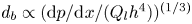 $d_b \propto ({\rm d} p/{{\rm d}\kern0.06em x} /(Q_l h^4))^{(1/3)}$ when assuming the pressure gradient to be homogeneous along the axial direction.
Another type of planar device has been studied by Castro-Hernández et al. (Reference Castro-Hernández, van Hoeve, Lohse and Gordillo2011). In their configuration the flow-focusing channel is rectangular, very long with respect to the channel width ( $l\sim 30w$) and considerably larger than the bubbles being produced. The stable gas thread remains attached to the upper PDMS wall. The model assumes the pressure gradient in the axial direction to be equal in the gas thread (with a constant gas flow rate) and the surrounding liquid. In the liquid, the pressure gradient is expected to decrease along the flow direction due to the development of the velocity profile from uniform at the entrance of the channel to parabolic downstream. Consequently, to match the pressure gradient in the liquid, the pressure gradient in the gas also decreases in the axial direction. This decrease is achieved by an increasing gas thread diameter
  $d_g$ which, according to the authors, triggers the bubble pinch-off. The assumptions of high Weber numbers and of constant gas flow rate allow the use of a relation between production rate, flow velocity and gas thread diameter,
  $f_b\propto U /d_g$, known from bubble pinch-off in a co-flow (Gordillo, Sevilla & Martínez-Bazán Reference Gordillo, Sevilla and Martínez-Bazán2007). Finally, exploiting (1.2), the resulting expression features a power law exponent
  $a=5/12$ and prefactor
 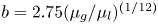 $b = 2.75 (\mu _g/\mu _l)^{(1/12)}$ that accounts for the gas and liquid viscosities, where
  $2.75$ is found empirically. The model disregards the fact that the gas ligament is attached to the wall and is thus embedded inside the liquid boundary layer, which leads to an overestimation of the liquid flow rate in particular for very thin gas threads.
While all these models assume the bubble production to be driven entirely by the pressure gradient, it is important to keep in mind that co-flow, or in other words, viscous entrainment, might play a role as well. For example, Quintero, Evangelio & Gordillo (Reference Quintero, Evangelio and Gordillo2018) summarize that (i) if the pressure gradient is dominant (also with respect to surface tension)
 \begin{equation} f_b \sim \sqrt{\frac{|\boldsymbol{\nabla} p|}{\rho d_b}} \quad \text{and} \quad d_b \sim \left( \frac{Q_g}{\sqrt{|\boldsymbol{\nabla} p|/\rho}} \right)^{2/5}, \end{equation}
while (ii) for co-flow, where the effect of the pressure gradient is negligible,
 \begin{equation} f_b \sim \frac{U}{d_g} \quad \text{and} \quad d_b \sim \left( \frac{Q_g d_g}{U} \right)^{1/3}. \end{equation}
In many real cases this also implies that much more complexity can be added in the presence of both effects.
Given the high level of complexity of the full problem, these models are bound to use simplifying assumptions that are more or less specific to a given geometry. Each of the studies presents models that agree well with the respective experimental measurements they aim to describe. Furthermore, and despite significant difference in the underlying physical principles that they are based upon, these models propose comparable power laws with an exponent near  $0.4$. Given limited experimental accuracy and operating range of the microfluidic chips, which typically do not exceed one order of magnitude, the subtle differences in power laws are insufficient to discriminate correct from potentially inaccurate conceptual approaches. This would require finer theoretical descriptions going beyond scaling law consideration and which account for the specific properties of the fluids used. Specifically, recent work (Cleve et al. Reference Cleve, Diddens, Segers, Lajoinie and Versluis2021) suggests that neglecting liquid viscosity and assuming a constant gas flow rate may not always be justified. Likewise, it was suggested that gas inertia has a role to play albeit during a short but meaningful fraction of the bubble formation process, i.e. close to the moment of pinch-off (Gordillo et al. Reference Gordillo, Sevilla, Rodríguez-Rodríguez and Martínez-Bazán2005; Dollet et al. Reference Dollet, Van Hoeve, Raven, Marmottant and Versluis2008), so that changes of the bubble size of approximately 10 % due to different gas densities between air and helium bubbles have been reported (Gordillo et al. Reference Gordillo, Sevilla and Martínez-Bazán2007). Once again, hindered by the complexity of the full problem, it is doubtful that a general analytical model with all experimentally relevant parameters can be conceived. Nevertheless, a broader experimental investigation of the parameter space may yet allow to narrow the relevant physical considerations without oversimplifying the problem.
3. Materials and methods
3.1. Experimental set-up
Experiments were conducted in flow-focusing devices, which were fabricated from two isotropically etched glass wafers, aligned and bonded together. The flow-focusing channel has a length  $l$ and its cross-section has a width
  $w$ and a height
  $h$ with rounded corners (radius of curvature
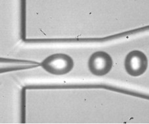
  $h/2$), see Cleve et al. (Reference Cleve, Diddens, Segers, Lajoinie and Versluis2021) and Segers et al. (Reference Segers, Gaud, Versluis and Frinking2018a) for more detail. Two different channel sizes were used, as shown in figure 1(a,b). The geometry and channel cross-section are depicted in figure 1(c).

Figure 1. (a) Snapshot of the short channel during bubble production with 42 % glycerol and 2 % Tween 80 in water and N $_2$ as the gas phase. (b) Snapshot of the long channel with DSPC/DPPE-PEG500 in saline and N
 $_2$ as the gas phase. (Saline is an isotonic solution of 0.9 % w/v NaCl in water, used for injection in the human body.) (c) Geometry of the flow-focusing channels with
  $w$ channel width,
  $h$ channel height,
  $S$ section area and
  $l$ channel length. Furthermore, the bubble diameter
  $d_b$ is indicated. (d) Schematic of the experimental set-up.
The chips were integrated in a stand-alone monodisperse bubble production system, as introduced by van Elburg et al. (Reference van Elburg, Collado-Lara, Bruggert, Segers, Versluis and Lajoinie2021). A schematic is presented in figure 1(d). The liquid was flow rate controlled (EL-FLOW series, Bronkhorst, NL) and the gas was pressure controlled (EL-PRESS series, Bronkhorst, NL). For the experiments reported here, the liquid flow rate ranged between 50 and  $250\,\mathrm {\mu }$l min
 $^{-1}$ and the gas pressure ranged between 1 and 3 bar overpressure. For the specific case of high liquid viscosity experiments, the gas pressure was increased up to 8 bar. The temperature of the whole production system could be increased up to
  $60\,^{\circ }{\rm C}$ to minimize the on-chip coalescence of phospholipid-coated bubbles (Segers et al. Reference Segers, Lassus, Bussat, Gaud and Frinking2019). In order to measure the production rate, the device is equipped with a low power (5 mW) laser module and a fast photodiode (FDS100, Thorlabs, Si detector, 350–1100 nm, 14 ns rise time and 13 mm
 $^2$ aperture), see van Elburg et al. (Reference van Elburg, Collado-Lara, Bruggert, Segers, Versluis and Lajoinie2021) for more details. Snapshots were recorded at 15 fps with a CCD camera (Lumenera LM165M,
  $1280\times 1024$ pixels with a pixel size of
  $6.45\,\mathrm {\mu }{\rm m}$ and equipped with a
  $15\times$ objective resulting in an image resolution of
  $0.44\,\mathrm {\mu }$m pixel
 $^{-1}$) illuminated using a LED flash light emitting a 100 ns light pulse for each frame.
The bubble volume was extracted from the images by volume integration assuming axisymmetry. From the volume the equivalent diameter of a spherical bubble was calculated. Bubbles positioned between 15 and  $30\,\mathrm {\mu }{\rm m}$ into the flow-focusing channel were evaluated, as this avoids increased motion blur due to very high velocities close to the inlet. Note that the final mean bubble diameter of lipid-coated bubbles is typically two to three times smaller once the bubbles have stabilized though diffusive dissolution, which mechanically compresses the initially loosely pact lipid shell (Segers et al. Reference Segers, Lohse, Versluis and Frinking2017). The bubbles produced in this study thus had relevant sizes for medical applications.
3.2. Experimental procedure
Bubble production using 10 different surfactant mixtures (phospholipid mixed with PEGylated phospholipid DSPC/DPPE-PEG5000, 9/1 molar ratio; DOPC/DPPE-PEG5000, 9/1; DMPC/DPPE-PEG5000, 9/1; pure DPPE-PEG5000; PEG40s; Tween 80; Tween 20; Sodium dodecyl sulphate; Zonyl FSO; Pluronic F68) and one without any surfactant were compared to investigate the effect of interfacial tension. Either Tween 80 or DSPC:DPPE-PEG5000, both showing a very similar effect on bubble production, were used by default when varying gas or liquid properties. Further experiments were conducted with glycerol concentrations of up to 50 % in water and with the surfactant Tween 80 to study bubble production under increased liquid viscosity. The gas used by default was N $_2$, however, measurements with three other gases (CO
 $_2$, SF
 $_6$ and C
 $_4$F
$_4$F $_{10}$) were also conducted to quantify the role of the gas properties on bubble production. Note, however, that the change of either surfactant, glycerol concentration or gas can simultaneously modify several physical fluid parameters. For instance, the addition of glycerol not only increases the liquid viscosity but also decreases the interfacial tension and increases the liquid density (Takamura, Fischer & Morrow Reference Takamura, Fischer and Morrow2012). Likewise, the addition of most surfactants can also increase liquid viscosity. Changing the gas leads to different gas densities, gas viscosities and interfacial tensions. Unless otherwise specified, all experiments with phospholipids were conducted at
  $60\,^{\circ }{\rm C}$ and all experiments without surfactants and with other types of surfactants at
  $40\,^{\circ }{\rm C}$.
For one measurement series (i.e. one specific combination of liquid, gas and temperature), we explored the full range of gas pressures and liquid flow rates for which stable bubble production with  $d_b< h$ in the jetting regime was possible. This operating regime was limited for low liquid flow rates by the possibility to stably create bubbles in the jetting regime itself, i.e. the regime where the gas jet remains inside the flow-focusing channel (and does not retract from the channel periodically such as in the dripping regime). Note, however, that the limiting conditions highly depended on the stability of the system, which could easily be affected by, e.g. dust particles. The minimum gas pressure required depends on the liquid flow rate but also on the liquid and gas properties, as it has to overcome the pressure drop inside the flow-focusing channel. For too low pressures, the gas flow would stop, and no bubbles would be produced. For high liquid flow rates, experiments were limited mostly by increased motion blur in the images. This also means that for some measurement points we can only present results for the production rate; production rate detection with the laser-photodiode system was reliable at any flow velocity. During the experiments the production rate was constantly monitored by which its stability was assured during each experiment consisting of a series of 90 images.
3.3. High-speed recording experiments
To enable a detailed discussion on bubble formation, we also recorded high-speed movies for a few experimental settings. The employed high-speed imaging set-up is described in detail in Cleve et al. (Reference Cleve, Diddens, Segers, Lajoinie and Versluis2021). This set-up does, however, not allow temperature regulation and real-time monitoring of the production rate. In short, the liquid was driven by a syringe pump (Harvard PhD) and the gas flow was pressure controlled (IMI Norgren). Imaging was achieved with an ultra-high-speed camera (Shimadzu HPV-X2) operated at a frame rate of 10 million frames per second with a resolution of  $400\times 250\,{\rm pixels}^{2}$ (imaging resolution
  $0.25\,\mathrm {\mu }$m pixel
 $^{-1}$). The total image magnification was
  $120\times$. Light was supplied by a Xenon strobe light (Vision Light Tech).
3.4. Numerical method
To support the experimental observations, we also conducted a series of numerical simulations. The numerical model used is explained in more detail in Cleve et al. (Reference Cleve, Diddens, Segers, Lajoinie and Versluis2021). In short, both the liquid and gas dynamics were modelled using the incompressible Navier–Stokes equation using sharp-interface arbitrary Lagrangian–Eulerian finite element scheme. The simulated domain is ‘two-dimensional’ assuming radial symmetry of the flow-focusing channel. This model was validated in terms of the bubble shape dynamics (formation and pinch-off), production rate, velocity of the bubbles and average and oscillatory velocity of the surrounding liquid (Cleve et al. Reference Cleve, Diddens, Segers, Lajoinie and Versluis2021). Note that, owing to the restriction of the axisymmetric geometry, the simulation cannot perfectly reproduce the non-axisymmetric experimental channel (see figure 1c), thereby displaying quantitative differences when compared with experimental results over a large parameter range. In the present study, this numerical model is used to qualitatively describe the influence of individually varied physical fluid properties on bubble production. To that end, all numerical results are discussed with respect to the reference case  $Q_l=100\,\mathrm {\mu }$l min
 $^{-1}$,
  $p_g=0.7$ bar
  $\rho _l=1000$ kg m
 $^{-3}$,
  $\rho _g=1$ kg m
 $^{-3}$,
  $\mu _l=1$ mPa s,
  $\mu _g=17.5\,\mathrm {\mu }$Pa s and
  $\sigma = 72$ mN m
 $^{-1}$. The numerical flow-focusing channel has a diameter of
  $18.4\,\mathrm {\mu }{\rm m}$ and a length of
  $30\,\mathrm {\mu }{\rm m}$, thus having similar dimensions as the experimental one (see short channel, figure 1c).
4. Experimental results
4.1. Channel geometry
Figure 2 shows the experimental results for the two channel geometries conducted both with water with the DSPC/DPPE-PEG5000 mixture and N $_2$. For both chips, the production rate depends strongly on the liquid flow rate, see figure 2(a). For a given liquid flow rate, several experiments with varying gas pressure were conducted, but all resulting production rates collapse on a single curve. Consequently, as long as the gas pressure was large enough to allow stable bubble production (typically of the order of 1 bar, but depending on the liquid flow rate and the liquid and gas properties), no significant influence of the gas pressure or gas flow rate was observed. For the same liquid flow rate, the production rate in the short channel is twice as high as in the long channel. This difference can partly, but not fully, be explained by the smaller channel sections of the short channel and correspondingly higher liquid flow velocities.

Figure 2. Experimental results for the two different channel sizes. All experiments are conducted with water containing the DSPC/DPPE-PEG5000 mixture and N $_2$ gas. Production rate and bubble size are shown as functions of the liquid flow rate in (a,b), respectively. Panel (c) shows the bubble size as a function of the gas to liquid flow rate ratio. The fitted power law features an exponent
  $a=0.38$ for both channels. The grey square corresponds to a numerical simulation (
 $\sigma =45$ mN m
 $^{-1}$ and otherwise the reference conditions given in § 3.4) and shows a good agreement.
As opposed to the production rate, the bubble size for a given liquid flow rate does not collapse on a single curve, i.e. it depends on the gas pressure, see figure 2(b). Note that with increasing flow rate smaller bubbles can be produced; the black line in figure 2(b) indicates this trend, it corresponds to the minimum bubble size as a function of the liquid flow rate and decreases linearly in the studied parameter range. Maximum bubble sizes were limited by the maximum set gas driving pressure and only bubbles smaller than the channel width were considered. In figure 2(c), the bubble size is furthermore plotted as a function of the gas to liquid flow-rate ratio  $Q_g/Q_l$. Following the general form used in the literature, a scaling law of the form
 \begin{equation} \frac{R_b}{w} = b \left(\frac{Q_g}{Q_l}\right)^a, \end{equation}
is fitted to the experimental results. For both geometries a factor  $a\approx 0.38$ and
  $b \approx 0.45\pm 0.05$ is found. For the normalization, the channel width
  $w$ yielded the best agreement for
  $b$ between the short and the long channel. However, other options such as the hydraulic diameter
  $d_{hyd} = 4 * S / P$ with
  $P={\rm \pi} *h + 2*(w-h)$ or an average diameter
  $d_{av} = (w+h)/2$ are still of the same order of magnitude and lie within approximately 10 % of each other.
4.2. Temperature
Experiments with Tween 80 in water and N $_2$ in the short channel were conducted for temperatures ranging from
  $40\,^{\circ }$C to
  $60\,^{\circ }$C. Even though most physical parameters vary slightly with temperature (see table 2), its effect on the bubble size or production rate was found to be small enough to be neglected in the following (see figure 3). Within the temperature range tested and with increasing temperature, the liquid viscosity decreases by approximately 25 %, the liquid density decreases by less than 1 % (based on Takamura et al. Reference Takamura, Fischer and Morrow2012), the gas density decreases by 7 % and the gas viscosity increases by approximately 5 % (Lemmon et al. Reference Lemmon, Bell, Huber and McLinden2022). Surface tension of pure water would decrease by approximately 5 %.

Figure 3. Experimental results in the short channel operated with water, Tween 80 and N $_2$ at different temperatures. Production rate and bubble size are shown as functions of the liquid flow rate in (a,b), respectively. (c) Bubble size as a function of the gas to liquid flow rate ratio.
Table 2. Effect of temperature on gas and liquid properties. All values are obtained from Lemmon et al. (Reference Lemmon, Bell, Huber and McLinden2022).

4.3. Gas composition
Changing the gas composition modifies primarily the gas density, but also the gas viscosity and surface tension. Surface tension has been shown to be affected by the presence of fluorocarbon gases (Krafft, Fainerman & Miller Reference Krafft, Fainerman and Miller2015). We have conducted a pendant-drop experiment and can confirm that using perfluorobutane (C $_4$F
$_4$F $_{10}$) instead of air decreases the surface tension of pure water by approximately 2 % and water with the DSPC/DPPEPEG5000 mixture by approximately 8 %.
The effect of changing the gas composition on bubble size and production rate is shown in figure 4. Gas properties are summarized in table 3. For the same liquid flow rate, smaller bubbles (approximately 30 %, figure 4b) and considerably larger production rates (approximately 60 %, figure 4a) are measured for C $_4$F
$_4$F $_{10}$ as compared with N
 $_2$. The combined effect (on bubble size and production rate) leads to a decrease in the prefactor of the power law (figure 4c). The same trend is observed for the short chip (see figure S1 in the supplementary material available at https://doi.org/10.1017/jfm.2023.704). It must be noted that a lower gas driving pressure was generally necessary for the higher gas densities. It is also noted that the minimum driving pressure required to start the production of bubbles typically decreased with increasing gas density (and gas viscosity). A possible explanation is that the higher density gases together with the extremely high gas velocities in the jet neck, see more details in § 5.3.1, provide a larger ‘inertial push’ capable of stabilizing the gas thread. Finally, it should be mentioned that the typical flow-rate ratio for bubble production decreases with increasing liquid flow rate, which can partly explain the convex shape for C
 $_4$F
$_4$F $_{10}$ in figure 4(a) due to the conservation of volume (1.2). This observation will be discussed in more detail in § 5.4 and figure 15.

Figure 4. Experimental results for four different gases. All experiments are conducted with the long channel and with the same liquid, water with the DSPC/DPPE-PEG5000 mixture. The production rate and bubble size as functions of the liquid flow rate are shown in (a,b), respectively. Panel (c) shows the bubble size with respect to the flow-rate ratio, including a fit with a power law. The exponent of the power law is  $a=0.38\pm 0.1$ for all cases, the pre-factors are
  $b=0.53$ for N
 $_2$,
$_2$,  $0.5$ for CO
 $_2$,
$_2$,  $0.48$ for SF
 $_4$ and
  $0.46$ for C
 $_4$F
$_4$F $_{10}$. While driving pressures associated with the experimental points for N
 $_2$ range between 2.75 and 3.75 bar, those for C
 $_4$F
$_4$F $_{10}$ range between 1.75 and 2.75 bar.
Table 3. Different gases used and their physical properties. All values are obtained from Lemmon et al. (Reference Lemmon, Bell, Huber and McLinden2022) for  $60\,^{\circ }$C and 1 bar. As will be discussed later, certain gases can further affect the surface tension between the gas and a given liquid.

4.4. Liquid: water–glycerol solutions
The viscosity of the continuous phase can be increased by adding glycerol, with a marginal increase in liquid density and decrease in surface tension, see also table 4. For example, a solution composed of water and 40 % glycerol is over three times more viscous than water, the density is increased by 10 % and surface tension decreased by 4 % (Takamura et al. Reference Takamura, Fischer and Morrow2012). Experiments have been conducted in both the short channel and the long channel, see figure 5. Interestingly, in the short channel, the production rate as a function of the liquid flow rate is not affected by the change in viscosity, as can be seen in the collapse of all data points in figure 5(a); the applied gas pressure has a minor influence. However, lower liquid flow rates are necessary to produce similar sized bubbles at higher viscosities, see figure 5(b). Together, these lead to a significant increase of the prefactor in the power law with an increase in liquid viscosity, see figure 5(c). For the long channel, despite difficulties to keep bubble production stable for high glycerol concentrations (the points are more scattered), one can observe that the production rate as a function of the liquid flow rate clearly increases with increasing liquid viscosity, see figure 5(d). As for the short channel, lower liquid flow rates are necessary to produce similar sized bubbles at higher viscosities, see figure 5(e). Different from the short channel, the prefactor of the power law for the long channel remains rather constant, see figure 5( f). In summary, an increase in liquid viscosity only significantly affects the size of the bubbles formed in the short channel and the production rate in the long channel.
Table 4. Physical properties of water–glycerol solutions used in the present study. Liquid viscosity is calculated based on Cheng (Reference Cheng2008), density and surface tension values are extrapolated from Takamura et al. (Reference Takamura, Fischer and Morrow2012). The values printed in grey are not used for figures 5 and 6.


Figure 5. Experimental results for different glycerol concentrations, with N $_2$ and Tween80 in the short channel at
  $40\,^{\circ }$C (a–c) and long channel at
  $60\,^{\circ }$C (d–f). The viscosity is shown in colour code, the values are also summarized in table 4. Theproduction rates are shown in (a,d), and the bubble sizes with respect to the liquid flow rate in (b,e). Panels (c, f) show the bubble size with respect to the flow-rate ratio including a fit with a power law.

Figure 6. Gas pressure vs liquid flow rate corresponding to the data in figure 5. (a,b) Correspond to the short channel at  $40\,^{\circ }$C, (c,d) to the long channel at
  $60\,^{\circ }$C. Panels (a,c) show the set experimental pressure, while in (b,d) the pressure is normalized by the liquid viscosity.
As expected, operating the chips with higher liquid viscosity requires a higher gas pressure for the same liquid flow rate, see figures 6(a) and 6(c). The pressure drop across the nozzle can be written as the contribution of 2 terms: the viscous (linear) pressure drop in the bubble production channel, that scales with  $\Delta p \propto \mu _l (Q_g+Q_l)$, and the geometric (entry) pressure drop, that scales with
  ${\rm \Delta} p \propto \rho Q_l^2$ (see Cleve et al. (Reference Cleve, Diddens, Segers, Lajoinie and Versluis2021) for more details). Thus, the linear pressure drop dominates for high viscosities. The cross-over between a dominant viscous pressure drop and a dominant geometric pressure drop can clearly be seen in figure 6(b), where the solid black lines depict the minimum pressures required to produce stable bubbles. No such transition is visible for the long channel, where the pressure drop is always dominated by viscous effects, figure 6(d).
4.5. Surfactants
The influence of the type of surfactant (see figure 7) is generally weaker than that of different gas and/or different glycerol concentrations. For the finer effect, the surfactants can be categorized in three groups (see summary in table 5). (i) When using mixtures of DSPC/DPPE-PEG5000, DOPC/DPPE-PEG5000, DMPC/DPPE-PEG5000 or Tween 80, (figure 7a–f) which all have a large molecular weight, no significant difference is observed with respect to pure water for the short channel. For the long channel, a slight shift of the bubble size is visible. (ii) For solutions with the low molecular weight surfactants DPPE-PEG5000, PEG40s and Zonyl FSO, (figure 7g–l) we observe a  $\sim$20 % increase in bubble production rate. For the DPPE-PEG5000 and PEG40s solutions this also results in a slight decrease in bubble size. For the long channel, this shift is less pronounced. (iii) In the presence of Tween 20, SDS and Pluronic F68 (figure 7m–r) we observe a range of production rates for a given liquid flow rate instead of one single value. Furthermore, in this group, the bubble sizes (figure 7n,q) are strongly shifted with respect to the case of pure water. The division into three groups is an aid for reading the figure and displays similar general features. A very strict separation is, however, not possible. In particular, the different behaviour in two channels alone already highlights the complexity of the entire process.

Figure 7. Experimental results for bubble production with different surfactant solutions in the short (a–c) and the long channel (d–f). All experiments have been conducted with N $_2$ and either at
  $60\,^{\circ }$C for phospholipids or
  $40\,^{\circ }$C for other surfactants. The surfactants presented in these panels are discussed as group (i) in the main text. Pure water is used as a reference.

Figure 7 The surfactants presented in these panels are discussed as group (ii) in the main text. Pure water is used as a reference.

Figure 7 The surfactants presented in these panels are discussed as group (iii) in the main text. Pure water is used as a reference.
Table 5. List of surfactants, their concentrations used in the experiments presented in figures 7 and 8 and surface tensions at room temperature obtained via a pendant-drop method.

 $^{\ast }$no visible difference for 10 and 20 mg ml
 $^{-1}$, no visible difference for water instead of saline
 $^{\ast \ast }$no visible difference for 0.5 % to 5 %
The main purpose of surfactants is to increase the lifetime of a bubble by reducing the interfacial tension between the gas and the liquid phases in order to stabilize the bubble against dissolution. Surfactants are also necessary to stabilize bubbles during their formation, i.e. without surfactants all bubbles would coalesce in the microfluidic chip. We have measured the surface tension with a pendant-drop experiment at room temperature a few seconds after the creation of the pendant drop. These measurements were performed for water and for the non-phospholipid surfactants and these agree with values found in the literature (Basu Ray et al. Reference Basu Ray, Chakraborty, Ghosh and Moulik2007; Bąk & Podgórska Reference Bk and Podgórska2016). In general, one can further expect that the surface tension is up to a few Nm m $^{-1}$ lower due to the increased temperature in the flow-focusing experiments with respect to the pendant-drop experiment (Phongikaroon et al. Reference Phongikaroon, Hoffmaster, Judd, Smith and Handler2005). We furthermore measured the surface tension of our DSPC/DPPE-PEG5000 solution at room temperature and a few seconds after drop formation and obtained approximately 53 mN m
 $^{-1}$. The temperature dependence of phospholipid solution on temperature is much higher (tens of mN m
 $^{-1}$) (Lee, Kim & Needham Reference Lee, Kim and Needham2001). On the other hand, it takes of the order of a minute to reach the final value. All in all, the value of 53 mN m
 $^{-1}$ should be taken with extreme care. During the very short time of bubble creation the surfactants are still mainly dissolved in the bulk and have little surface active effects. (Some surfactants are certainly already present on the gas cusp, but the gas–liquid interface is considerably increasing during bubble pinch-off, which makes it likely that the surfactants are far from tightly packed during bubble pinch-off.) Bubble production frequencies are plotted as a function of the steady-state surface tension for a fixed liquid flow rate
  $Q_l = 100\,\mathrm {\mu }$l min
 $^{-1}$, see figure 8. It is interesting to note that, in general, the production rate decreases with increasing surface tension. As the values for DSPC follow the general trend, we have included it in the representation. Yet, we should once more recall the above discussed limits and uncertainties involved in obtaining this value.

Figure 8. Range of bubble production rates (represented by the vertical lines) found for  $Q_l=100\,\mathrm {\mu }$l min
 $^{-1}$ in figure 7(a,g,m) as a function of the surface tension of the liquid and air interface, measured at room temperature in a pendant-drop experiment. The limits of these values due to different temperatures and time scales are discussed in the main text. The simulated data (see also figure 10b) will be discussed in § 5.3.
5. Discussion
5.1. Preliminary consideration
Before discussing in detail the influence of the different parameters on the bubble production, we first need to include short considerations on the power law and expression for the production rate. Solving (1.1) and (1.2) for the production rate, one obtains
 \begin{equation} f_b\sim Q_g^{1-3a} Q_l^{3a}. \end{equation}
If the  $a= 1/3$, then the influence of the gas flow rate on the production rate cancels out and
  $f_b\sim Q_l$.
For the experimentally obtained power law exponent, one should bear in mind that, first, the flow-rate ratio only varies by one order of magnitude within the stable operating range of the chip and, second, we deduce the gas flow rate from the bubble size and production rate. Furthermore, practical limitations (e.g. resolution, motion blur, uncertainties in the driving condition, etc.) do not allow for making a statistically relevant distinction between a  $1/3$ or
  $2/5$ power law. However, let us consider the case of
  $a\approx 0.38$ as was found in figure 2(c). On the one hand, this implies a weak dependence on the gas flow rate (
 $\,f_b \sim Q_g^{-0.14}$). On the other hand, the expected dependence on the liquid flow rate is a power function leading to a slightly convex curve (
 $\,f_b\sim Q_l^{1.14}$). While obviously these models are simplified, they can partly explain that (i) the production rate as a function of the liquid flow rate is close linear or slightly convex, and that (ii) the dependence on the gas flow rate seems to be mostly negligible.
5.2. Pressure drop due to channel geometry
As discussed in the introduction, the pressure gradient has been identified as an important ingredient for bubble pinch-off in many previous papers. Castro-Hernández et al. (Reference Castro-Hernández, van Hoeve, Lohse and Gordillo2011) base their model on the comparison between the viscous pressure loss in the gas and liquid. Rodríguez-Rodríguez et al. (Reference Rodríguez-Rodríguez, Sevilla, Martínez-Bazán and Gordillo2015) discuss the significance of the changing sign in pressure between bubble growth and detachment, Evangelio et al. (Reference Evangelio, Campo-Cortes and Gordillo2015) try to find an optimal description of the pressure gradient for each of their considered cases. From our previous paper (Cleve et al. Reference Cleve, Diddens, Segers, Lajoinie and Versluis2021), we know that the pressure variation in the inlet region scales as  ${\rm \Delta} p \sim \rho _l Q_l^2 / S^2$, with
  $S$ being the cross-sectional surface area, and the viscous pressure loss along the channel as
  ${\rm d} p/{{\rm d}\kern0.06em x} \sim \mu _l Q_l/S^2$ (see also more detailed explanation in the supplementary material). By plotting the bubble size and production rate as a function of
  $Q_l/S^2$ (instead the previously used
  $Q_l$), we can obtain a perfect match between the data for the short and long channel from figure 2, see figure S3 in the supplementary material. This correction factor of
  $1/S^2$ thus points towards a dominance of the viscous pressure loss. However, having only data for two different channels does not allow for a decisive conclusion.
5.3. Liquid and gas properties
The observations from § 4 highlight differences in the behaviour of the flow-focusing devices when changing the liquid and/or gas. The changes operated for this investigation were chosen to affect predominantly one physical quantity. They do, however, affect other parameters, albeit to a lower degree. For instance, using a different gas implies different gas densities, different gas viscosities and possibly different interfacial tensions. Therefore, in order to support the experimental hypotheses qualitatively, we have conducted a series of numerical simulations where it is possible to vary a single parameter at a time. Some typical snapshots are presented in figure 9, a summary of all numerical results showing the influence of different parameters on the production rate and bubble size is plotted in figure 10. As far as possible, all parameters except one are kept constant, however, for certain simulations the gas pressure had to be adapted in order to keep the system in the relevant bubbling regime (jetting). The different parameters will be discussed together with experimental and theoretical aspects in the following subsections.

Figure 9. Three characteristic bubble shapes and gas flow fields for the reference case (a) and for five cases (b–f) with exactly one liquid or gas parameter modified with respect to the reference case. The exact values are reported in figure 10. An enlarged version of the images of (c) to highlight the zones of recirculation is included in figure S4 in the supplementary material. Movies are included in the supplementary material (V1 to V6).

Figure 10. Dependence of the production rate and bubble size with respect to different parameters. For all simulations, the same liquid flow rate  $q_l=100\,\mathrm {\mu }$l min
 $^{-1}$ was used. The gas driving pressure
  $p_g$ was kept constant if possible, but had to be adjusted for some simulations in order to remain in the bubbling regime. (Note that the
  $y$-axis of
  $p_g$ is different for ( f).) The reference point indicated by the red square ‘ref’ is the same in all plots, the purple triangles indicate the cases plotted in figure 9.
5.3.1. Gas properties: density and viscosity
In our experiments, gas density and gas viscosity were varied by changing the gas, as reported in § 4.3. The largest variation of a physical parameter can be achieved for the gas density, with a factor ten between the lightest, N $_2$, and the heaviest gas, C
 $_4$F
$_4$F $_{10}$. With increasing gas density, the production rate increases significantly and the bubble size decreases slightly, see figure 4. The numerical simulations in figure 10(c) qualitatively confirm this trend. An increase of the production rate and a decrease of the bubble size has also been observed experimentally and numerically for bubble generation in a co-flow device under a constant gas pressure by Gordillo et al. (Reference Gordillo, Sevilla and Martínez-Bazán2007). By comparing boundary-integral method simulations (with a constant gas flow rate) with their experiments, the authors concluded that gas inertia plays an important role in the final moments before pinch-off, and simulations were only matching experiments when gas inertia (meaning gas convective terms) was taken into account. As shown in figure 9 and reported in Cleve et al. (Reference Cleve, Diddens, Segers, Lajoinie and Versluis2021), our numerical simulations show velocities up to hundreds of metres per second in the gas just before pinch-off, which implies that the kinetic energy of the gas exceeds that of the surrounding liquid. This can act as an impulse to bubble formation, accelerating the pinch-off and leading to zones of recirculation inside the bubble, see figure 9(c) and a more detailed representation in figure S4 in the supplementary material. Gekle et al. (Reference Gekle, Peters, Gordillo, van der Meer and Lohse2010) experimentally and numerically confirm the presence of such high gas velocities during bubble pinch-off, albeit in a quiescent liquid and a much larger system. By studying the dynamics of the jet neck during pinch-off, Gordillo et al. (Reference Gordillo, Sevilla, Rodríguez-Rodríguez and Martínez-Bazán2005) and Dollet et al. (Reference Dollet, Van Hoeve, Raven, Marmottant and Versluis2008) found that the collapse of the jet neck in the last moments before pinch-off is accelerated and they attribute this to the high gas velocities inducing ‘Bernoulli suction’, which accelerates the liquid inward (Gekle et al. Reference Gekle, Peters, Gordillo, van der Meer and Lohse2010). In conclusion, most previous studies and the work presented here suggest that gas inertia is not negligible and has a particularly large effect around the moment of pinch-off, leading to overall variations (up to doubling) of the production rate and bubble size.
The bubble size can also be partly influenced by the differences in driving pressure that are necessary for the different gases. As reported above, higher density gases require a lower driving pressure. Consequently, the pressure drop in the entrance region and along the channel will be lower and the corresponding dilatation of the gas volume will be lower as well.
Lastly, one shall mention for completeness that the solubility of the gases differs per gas type and with increasing pressure, leading potentially to different gas saturation in the gas–liquid boundary layer and thus influencing the surface tension. However, even for a system at equilibrium the decrease of surface tension induced by increased pressure is less than 1 % (Masterton, Bianchi & Slowinski Reference Masterton, Bianchi and Slowinski1963). Furthermore, diffusion time scales are expected to be large with respect to the residence time of the liquid and gas in the flow-focusing region.
Gas inertia (due to different gas densities) is a likely candidate to explain another observation arising in both the numerical (compare figures 9(c) and 9(a)) and experimental high-speed imaging data (compare figure 11a,b). A downstream shift of the position of pinch-off into the channel is evident for higher density gases. A close look at the gas flow field in figure 9(c) (see also zoom provided in the supplementary material S4) further highlights that, even though maximum velocities are slightly lower for the higher density gas, inertial effects lead to visible re-circulation zones within the bubble. The now significant ‘inertial push’ of the gas is therefore likely to induce an increase in production rate and a decrease in bubble size by accelerating bubble detachment from the gas thread.

Figure 11. High-speed recording with (a) Tween 80 in water and air (close to reference case as air consists mainly of N $_2$), (b) Tween 80 in water and C
 $_4$F
$_4$F $_{10}$ and (c) water with 47 % glycerol and air. All experiments were performed at room temperature.
Numerically, an increase in gas viscosity results in a slight increase in production rate and a decrease of the bubble size (figure 10d) as well as a few micrometre upstream displacement of the pinch-off location, figure 10(d). This trend is opposite to our experimental observations, where the highest viscosity gas N $_2$ leads to the lowest productions rates and largest bubble sizes, cf. figure 4. Consequently, we can conclude that the experimental observations are dominated by gas density, and not by gas viscosity.
The only model available in the literature that considers gas viscosity is the one by Castro-Hernández et al. (Reference Castro-Hernández, van Hoeve, Lohse and Gordillo2011). With a 50 % increase in viscosity their model would predict a 3 % increase in bubble size and a 9 % decrease in production rate, which is also opposite to our numerical simulations. Let us, however, recall that their model neglects gas inertia and is based upon a long and stable gas jet, which is different from our experimental observations.
5.3.2. Liquid properties: viscosity and density
Liquid viscosity is the parameter most frequently discussed in the context of flow focusing, albeit mainly in the squeezing regime. In flow configurations closer to ours, where the bubble is only filling a part of the channel, viscosity has been explicitly considered by Castro-Hernández et al. (Reference Castro-Hernández, van Hoeve, Lohse and Gordillo2011) and Evangelio et al. (Reference Evangelio, Campo-Cortes and Gordillo2015). Viscosity has two main effects: (i) increasing the pressure drop along the channel (and thus indirectly having an effect on the compressible gas phase) and (ii) influencing the balance between viscous and inertial forces as expressed through the Reynolds number. The model by Castro-Hernández et al. (Reference Castro-Hernández, van Hoeve, Lohse and Gordillo2011) only takes into account the pressure drop and predicts an impact on the bubble size that scales as  $d_b \propto 1/\mu _l^{1/12}$. The model by Evangelio et al. (Reference Evangelio, Campo-Cortes and Gordillo2015) takes into account both aspects. The expression used for the pressure gradients depends on the viscosity and on the position of bubble pinch-off. For high viscosities, the authors numerically find a pressure gradient
  $\mathrm {d}p/\mathrm{d}\,x=-32\mu _l U /L^2$. They furthermore consider either the viscous or the inertial term of the Rayleigh–Plesset equation for describing the bubble itself. They subsequently derive four semi-empirical models for different viscosity ranges. Differently from these studies, the experimental bubble sizes reported by Gañán-Calvo (Reference Gañán-Calvo2004) all collapse on a single curve independently of the liquid viscosities which vary by a factor 50. Numerical studies by Jia & Zhang (Reference Jia and Zhang2020) and Chekifi et al. (Reference Chekifi, Boukraa and Aissani2021) on the other hand report an increase of the production rate and decrease of the bubble size for increasing viscosity in the squeezing regime.
Our experimental results cover a small range of liquid viscosities: a factor 5 between the largest and smallest ones. Even for the highest viscosity and lowest flow rates the liquid Reynolds number is above 10. The above models therefore do not predict any significant influence of liquid viscosity on the bubble production within our experimental parameter space. Yet, our experimental results (see figure 5) show either an increase of the bubble size in the short channel (increase of the prefactor of the power law), or an increase of the production rate in the long channel. The simulations suggest an increase in production rate for increasing liquid viscosity and for a more or less constant bubble size, see figure 9( f). For practical applications it is interesting to note that, with increased liquid viscosity, one can make smaller bubbles at lower liquid flow rates (figure 5b).
A few more minor observations are worth mentioning. In particular, in figure 5(a), the production rate depends no longer on the liquid flow rate alone. A possible reason is the rather large and long bubbles (see also figure 11c), together with the increased viscosity, which lead to a large variation of the pressure gradient close to the wall. Furthermore, the frequency sometimes displays a hysteresis effect, which makes the different experimental runs (with each a fixed pressure while gradually increasing the liquid flow rate) easily distinguishable (see flattened out data points in figure 5a). A very similar behaviour can also be observed in other chip configurations (Dhanaliwala et al. Reference Dhanaliwala, Chen, Wang and Hossack2013).
Liquid density does not appear in any of the models cited above, despite the fact that it appears in the summarized (2.3a,b) by Quintero et al. (Reference Quintero, Evangelio and Gordillo2018). Indeed, Rodríguez-Rodríguez et al. (Reference Rodríguez-Rodríguez, Sevilla, Martínez-Bazán and Gordillo2015) and Evangelio et al. (Reference Evangelio, Campo-Cortes and Gordillo2015) (for the inertia dominated case) replace the pressure gradient by the momentum equation which makes the density cancel out naturally. In the dimensional analysis by Gañán-Calvo (Reference Gañán-Calvo2004), liquid density has been neglected. This was justified by (i) the density being of the order of one and (ii) by the fact that, within their analysis, modifying the liquid density slightly would have no effect on the final power law. As explained above, the models by Castro-Hernández et al. (Reference Castro-Hernández, van Hoeve, Lohse and Gordillo2011) and Garstecki et al. (Reference Garstecki, Gitlin, DiLuzio, Whitesides, Kumacheva and Stone2004) differ entirely from (2.3a,b): no liquid density is taken into account. In the most extreme cases in the literature, the addition of glycerol to the water leads to liquid density changes of up to 7 % (Evangelio et al. Reference Evangelio, Campo-Cortes and Gordillo2015), which is considerably smaller than the change in liquid viscosity. Our simulations, figure 10(e), suggest that an increased liquid density slightly decreases both the production rate and the bubble size.
5.3.3. Interfacial tension
Analytical models found in the literature usually argue that surface tension has to be overcome to produce the bubbles, but the parameter usually disappears in the final model. In an experimental study, Garstecki et al. (Reference Garstecki, Gitlin, DiLuzio, Whitesides, Kumacheva and Stone2004) reported explicitly that a twofold decrease of the surface tension (using Tween 20) had no effect on the bubble size in their squeezing regime experiments. Also Hettiarachchi et al. (Reference Hettiarachchi, Talu, Longo, Dayton and Lee2007), did not report on any differences when using various surfactants. Numerical simulations by Chekifi et al. (Reference Chekifi, Boukraa and Aissani2021), however, suggest a decrease of the bubble size with increasing surface tension, which is in line with our experimental and numerical trends, see figures 7 and 10(b), (the slight increase of bubble size in figure 10(b) is mainly due to the higher gas pressure). Gordillo et al. (Reference Gordillo, Sevilla and Martínez-Bazán2007) observed experimentally that, for bubble pinch-off in co-flow, a decrease of the Weber number (i.e. an increase of the surface tension) leads to an increased production rate. This trend is in contradiction with both our numerical simulations (figure 10b) and most of our experimental findings (figures 7(a,g,m) and 8) where a decrease in surface tension leads to an increase in production rate.
While in the numerical simulations the effect of surface tension on the production rate is pronounced, in the experiments the role of changing surface tension is much lower. A notable difference between the two is that, in the simulation, surface tension is constant and applies to all gas–liquid boundaries. In the experiments, the surface area is changing very rapidly as the surfactants adsorb on the newly created interface. It is questionable that surfactants can form a tightly packed monolayer at the time scale of the bubble production process. This aspect is far from trivial. The values generally reported are equilibrium values. The time needed to reach this equilibrium depends on the surfactant and is estimated based on diffusion alone, if at all a relevant factor for such short time scales. The present case of a flow-focusing device includes a strong convective component, which makes predicting the steady-state time for surfactant adsorption very challenging. It remains, however, probable that the time scales are too short to entirely reach this equilibrium before pinch-off. For phospholipids, stabilization of bubbles only after partial dissolution (Segers et al. Reference Segers, De Rond, de Jong, Borden and Versluis2016, Reference Segers, Lohse, Versluis and Frinking2017, Reference Segers, Lassus, Bussat, Gaud and Frinking2019; Zalloum et al. Reference Zalloum, Paknahad, Kolios, Karshafian and Tsai2022) demonstrates that the phospholipid layer is, indeed, far from fully packed.
The role of the gas–liquid interface is further complicated by considering surface elasticity, i.e. the response of the surface to stresses induced by its deformation (Cantat et al. Reference Cantat, Cohen-Addad, Elias, Graner, Höhler, Pitois, Rouyer and Saint-Jalmes2013). The classical definition of surface elasticity is  $\chi = A \,\mathrm {d}\sigma / \mathrm {d}A$, which has been shown to be a satisfactory description for oscillating bubbles with a phospholipid monolayer in the elastic regime between buckling (surface area gets too small) and break-up (surface area gets too large) (Marmottant et al. Reference Marmottant, Van Der Meer, Emmer, Versluis, De Jong, Hilgenfeldt and Lohse2005). However, the change of surface area during bubble formation is not uniform (particularly in the jet neck), which can induce counteracting restoring forces (Cantat et al. Reference Cantat, Cohen-Addad, Elias, Graner, Höhler, Pitois, Rouyer and Saint-Jalmes2013). On the other hand, phospholipid surfactant bubbles are known to considerably shrink after formation until reaching a stable size with full surfactant packing (Segers et al. Reference Segers, De Rond, de Jong, Borden and Versluis2016, Reference Segers, Lohse, Versluis and Frinking2017). At the moment of pinch-off they are thus far from fully packed, which therefore considerably reduces any effect of surface elasticity.
Amongst the surfactants considered, the most spectacular effects appear with Pluronic (see also figure S2 in the supplementary material). The production rate is much higher than for the other surfactants. Pluronic is known to be extremely shear thinning and to have strong viscoelastic properties, which may be the cause of this observation. This aspect is beyond the scope of our study but is interesting enough to warrant further investigation.
5.3.4. Discussion of the influence of the gas and liquid physical parameters
To summarize the above discussion, we have conducted a set of further numerical simulations where both the gas density and gas viscosity have been set to the values of N $_2$, CO
 $_2$, SF
 $_6$ and C
 $_4$F
$_4$F $_{10}$. In figure 12 we are comparing those with our experimental data. The same trend for the simulated and experimental results are found, but differences in the absolute values remain. As discussed in the different sections above, this can be linked to a number of different reasons. Among the most important factors are (i) the differences in channel geometry between the experimental and numerical channel, (ii) the difficulty of correctly assessing the surface tension in experiments and its possible variation over space and time (which are also visible in the different behaviours between the short and the long channel, see figure 7) and (iii) the fact that numerical simulations are conducted assuming incompressibility while at the moment of pinch-off the very high gas flow velocities will undoubtedly induce some compression in the experimental case. Nonetheless, the generally good agreement between the trends of both approaches allowed us to make a fair comparison. In that sense, the experimental and numerical data are complementary, as the first give an overview of the complex situation of the real system, while the second allow us to investigate otherwise inaccessible details but in a simplified system.

Figure 12. Comparison of the experimental production rate with different gases in the short channel (data from figure S1 in the supplementary material) with numerical simulations. Note that, for each simulation, both the gas density ( $x$-axis) and gas viscosity (not shown but corresponding to the respective gas) have been modified. Also note that the gas pressure has been slightly adjusted to remain in a stable regime of bubble production.
5.4. Comparison with the existing theoretical models
In the following, we compare our experimental results with four of the models from the literature discussed in § 2. As Gañán-Calvo (Reference Gañán-Calvo2004) and Rodríguez-Rodríguez et al. (Reference Rodríguez-Rodríguez, Sevilla, Martínez-Bazán and Gordillo2015) give the same results for the bubble size, we treat them together, taking the pre-factor  $b=1.1$ proposed by Gañán-Calvo (Reference Gañán-Calvo2004). For the production rate we take the expression derived by Rodríguez-Rodríguez et al. (Reference Rodríguez-Rodríguez, Sevilla, Martínez-Bazán and Gordillo2015), see table 1. Their expression for the production rate includes an unknown scaling factor, which leads to the best agreement with our experiments for both channel geometries when set to
  $c\approx 1.5$. The second model we consider is that by Castro-Hernández et al. (Reference Castro-Hernández, van Hoeve, Lohse and Gordillo2011), we, however, use an adapted expression for the bubble size: multiplying their expression with
  $0.5$ (thus using a pre-factor
  $0.5\times 2.75$) as this leads to a good agreement with our data (while the original expression does not give an agreement, most likely due to different liquid flow velocities around the gas jet, which is attached to the wall in the study by Castro-Hernández et al. (Reference Castro-Hernández, van Hoeve, Lohse and Gordillo2011) and in the channel centre in our work). For the production rate a pre-factor
  $c\approx 0.5$ gives the best agreement for both channel geometries. From the work by Evangelio et al. (Reference Evangelio, Campo-Cortes and Gordillo2015) we use the two versions corresponding to their low viscosity experiments, (ii) for
  $Q_g/Q_l<0.1$ and (iii) for
  $Q_g/Q_l>0.1$. As all pre-factors are defined in the model, no additional scaling parameter is needed.
Since the production rate is a function of several parameters, particularly of  $Q_g$ and
  $Q_l$, it is difficult to plot theoretical predictions without fixing one of these parameters. On the other hand, both parameters are varying in our experiments. Nonetheless, one can use the experimentally measured flow rates as input parameters and calculate the predicted bubble sizes
  $R_b$ and production rates
  $f_b$ for every model. In figure 13 we compare those predictions (
 $y$-axis) with the actually measured ones (
 $x$-axis). Points located on the black line correspond to a perfect correspondence between measurement and prediction (
 $R_{\textrm{calculated}}=R_{\textrm{measured}}$ or
  $f_{\textrm{calculated}}=f_{\textrm{measured}}$). The data sets chosen are those of figure 2 (N
 $_2$ and phospholipid solution), which have been taken as reference data throughout this document. The upper row (a–d) shows the bubble sizes, the lower row (e–h) the production rates. All models show a reasonable agreement, but there is a clear discrepancy between the short and long channels; all models predict that the short channel will produce larger bubbles (figure 13a–d) at lower production rates (figure 13e–h). A possible reason for this is that the channel geometry is not cylindrical in our experiments. We have used
  $D=2\sqrt {S/{\rm \pi} }$ as this yields the best results compared with the channel height or channel width alone. The plot can be slightly improved by using somewhat modified channel sizes (see figure S6 in the supplementary material) but this fine tuning appears very artificial. No model obviously stands out in figure 13. As discussed above, our specific channel geometry is a possible culprit.

Figure 13. Comparison of the experimentally obtained bubble size  $R_{\textrm{measured}}$ (a–d) and the experimentally obtained production rates
  $f_{\textrm{measured}}$ (e–h) from figure 2 (respective
  $x$-axes) with the predictions from different models (
 $R_{\textrm{calculated}}$ or
  $f_{\textrm{calculated}}$ on the respective
  $y$-axes). For the predicted values, we use our experimental flow rates and channel geometries as input parameters in the theoretical models from table 1. The distance to the identity line (
 $x$-value equal to
  $y$-value) thus directly shows the difference between the model and the experiments. Points above the line are overestimated by the model while points below the line are underestimated by the model. Thus, most predictions show the same trend, yet without perfectly matching the experimental results. Note that the bubble size predicted by Castro-Hernandez has been multiplied by a factor 0.5 (‘adjusted’) in order to fit to our results. The values of
  $c$ in (e, f) are pre-factors chosen to obtain a best fit.
A closer investigation of all available models reveals, however, some general discrepancies with respect to our experimental results. Figure 14(a) compares the production rate, figure 14(b) the bubble size as a function of the liquid flow rate and figure 14(c) the bubble size as a function of the flow-rate ratio. As all models define the bubble size in the form of (1.1), we would expect the bubble size to only depend on the gas to liquid flow-rate ratio. However, as highlighted in figure 14(b), the bubble size for  $Q_g/Q_l=0.3$ (red data points) is decreasing for increasing liquid flow rate. For the production rate, the inverse observation is true: while experiments show only a dependency on the liquid flow rate, all theories predict a dependency on the bubble size or gas flow rate (see expressions in table 1). For this reason, we chose for the comparison a fixed ratio
  $Q_g/Q_l=0.3$, figure 14(a), which gives a linear relation for all models. As discussed in § 5.1 and visible in figure 14(a), also the experimental relation is close to linear. We can see, however, that a fit does not go through the origin. Consequently, the order of magnitude between experiments and models is the same, the real situation is, however, more complex than in the simplified models. However, considering a fixed flow-rate ratio does not account for the effective operating range of the chips: a gas to liquid flow-rate ratio of 0.3 is not achievable for every liquid flow rate. figure 15(a) reveals that the typically acceptable flow-rate ratio decreases with increasing liquid flow rate (the same holds for the minimum flow-rate ratio necessary to produce bubbles). In figure 15(a), we therefore plot a trendline to represent this behaviour, which consists of a second-order polynomial. Plugging this trendline into the theoretical expressions for the production rate of the different models does result in a better agreement between experimental data and theoretical predictions. This is no surprise, as we indirectly apply (1.2). While, for a given channel geometry, low liquid flow rates allow for larger gas to liquid flow-rate ratios (and thus less waste of liquid) and lower operating pressures, higher liquid flow rates allow for production of more and smaller bubbles.

Figure 14. Comparison of our reference data (figure 4) for the short channel with models from the literature. Each panel shows experimental data (black data points), experimental data for the range  $0.27< Q_g/Q_l<0.33$ (red data points), a linear fit through these points and different theoretical predictions (with
  $Q_g/Q_l = 0.3$ fixed for (a,b)). (a) Production rate as a function of the liquid flow rate. For the adjusted Castro-Hernandez model we have multiplied the bubble size by a factor 0.5 in order to fit to our results. (b) Bubble size as a function of the liquid flow rate. As in figure 13 we have used a pre-factor
  $c=1.5$ for the Ganan-Calvo/Rodriguez-Rodriguez model and
  $c=0.5$ for the Castro-Hernandez model. (c) Bubble size as a function of the gas to liquid flow ratio. The same trends can be confirmed by data for the long channel (see figure S7 in the supplementary material).

Figure 15. (a) Gas to liquid flow-rate ratio as a function of the liquid flow rate. A trend line is fitted to the data. (b) Production rate as a function of the liquid flow rate. The experimental data are compared with the theoretical models, in which we applied the trend line from (a) for the ratio  $Q_g/Q_l(Q_l)$. The same trends can be confirmed by data for the long channel (see figure S8 in the supplementary material).
6. Conclusions
In the present study we have conducted a detailed analysis of the role of gas and liquid properties in the size and production rate of micrometre-sized gas bubbles produced in a flow-focusing device. For a fixed liquid flow rate, the gas density has a strong effect on the production rate while liquid viscosity influences most severely the bubble size. A decreased surface tension tends to increase the production rate, but strong conclusions in that regard are difficult as the equilibrium surface tension is probably not reached at or within the time scale of bubble formation.
In most cases, for our flow-focusing devices, the production rate only depends on the liquid flow rate and the dependency is close to linear. This relation leads to a power law of the order of  $1/3$, which is close to the values proposed in the literature. We have compared our experimental results in more detail with some of these models. While the general trends can be reproduced by any of them, the details are not captured by any of the models due to the experimental complexity. The large variety in applied flow-focusing devices further complicates the elaboration of a universal model. Nevertheless, our results can be taken as a guideline for predicting the impact of gas and liquid properties when designing new flow-focusing configurations.
Supplementary material and movies
Supplementary material and movies are available at https://doi.org/10.1017/jfm.2023.704.
Acknowledgements
The authors thank P. Bussat and R. Melich for insightful discussion.
Funding
This project is partly financed by Holland High Tech with a public–private partnership allowance in the top sector High Tech Systems and Materials (HTSM) and by Bracco Suisse S.A. The following co-authors further acknowledge funding: G.L. from the 4TU Precision Medicine program supported by High Tech for a Sustainable Future, a framework commissioned by the four universities; and T.S. from the Max Planck – University of Twente Center for Complex Fluid Dynamics.
Declaration of interests
The authors report no conflict of interest.
Data availability statement
The data that support the findings of this study are available from the authors upon reasonable request.
Author contributions
S.C., G.L., T.S., M.V. and S.C. designed the experiment. S.C., B.E. and E.G. set up the experiment. A.L. prepared the material. S.C. conducted the research. C.D. and S.C. performed numerical simulations. S.C., G.L., T.S. and M.V. wrote the manuscript.


 Open access