


1 Introduction
The exhaust of jet engines continues to be a significant contributor to aircraft noise. The problem is particularly acute for medium-bypass ratio, high-performance turbofan engines that are envisioned to power the next generation of supersonic transports. Even for large-bypass ratio engines on commercial subsonic aircraft, jet noise remains a problem and an active area of research. For fixed engine cycle, jet noise reduction is achieved through some sort of modification of the exhaust nozzle. Such modifications have included chevrons (Brown, Bridges & Henderson Reference Brown, Bridges and Henderson2011), fluidic injection (Henderson Reference Henderson2010; Powers, McLaughlin & Morris Reference Powers, McLaughlin and Morris2015), plasma excitation (Samimy et al. Reference Samimy, Kim, Kastner, Adamovich and Utkin2004) and offset-stream nozzles (Papamoschou & Debiasi Reference Papamoschou and Debiasi2001; Papamoschou Reference Papamoschou2004; Henderson Reference Henderson2012; Papamoschou, Xiong & Liu Reference Papamoschou, Xiong and Liu2014; Henderson, Leib & Wernet Reference Henderson, Leib and Wernet2015; Huff & Henderson Reference Huff and Henderson2016; Papamoschou et al. Reference Papamoschou, Phong, Xiong and Liu2016), the last having motivated the present study. These approaches have been subjected to numerous experimental and computational investigations. Computational tools like large eddy simulation (LES) have progressed to the point where they can provide high-fidelity, time-resolved solutions to the flow field (Bridges & Wernet Reference Bridges and Wernet2012). Combined with surface integral methods, these computations yield far-field noise spectra that are becoming increasingly reliable (Brès et al. Reference Brès, Ham, Nichols and Lele2017). However, the high computational cost, long turnaround times and enormity of data sets associated with LES-based approaches render them impractical for design purposes. There is need for low-order tools that can provide rapid guidance to the designer of exhaust systems regarding their potential to reduce noise. The robustness of such tools hinges on capturing the salient physics of noise generation and noise reduction. Identifying the salient physical processes of noise reduction is relevant not only to the development of rapid prediction tools but also to the interpretation of the vast data sets generated by experiments and time-resolved computations. It is therefore the goal of this effort to provide the framework of a physics-based methodology for the treatment of complex nozzle configurations considered for advanced flight vehicles.
The predominant low-order modelling tool used today consists of an acoustic analogy coupled with a Reynolds-averaged Navier–Stokes (RANS) solution of the flow field. The original acoustic analogy formulation by Lighthill (Reference Lighthill1952) uses the free-space Green’s function and can yield satisfactory results for round jets (Morris & Farassat Reference Morris and Farassat2002). Improvements have included the effect of refraction by the mean flow, which requires solving the linearized Euler equations (Morris & Boluriaan Reference Morris and Boluriaan2004; Goldstein & Leib Reference Goldstein and Leib2008). Simplification is often sought through the locally parallel-flow approximation, in which case the Green’s function can be reduced to analytical forms. This approach has yielded accurate predictions for jets from round nozzles as well as nozzles with chevrons and fluidic injection (Depuru Mohan & Dowling Reference Depuru Mohan and Dowling2016). For the chevron and fluidic-injection jets, azimuthal effects on propagation were not considered, which is a reasonable simplification given that the mean flow is mostly axisymmetric.
For asymmetric jets, inclusion of refraction effects becomes a much larger challenge. Yet, it is critical to account for them in some fashion in order to capture the azimuthal variation of noise emission and the noise suppression enabled by offset-stream concepts. Even under the simplification of the parallel-flow approximation, the construction of the Green’s functions involves complex numerical procedures (Leib Reference Leib2014). The parallel-flow approximation itself poses the risk of disregarding flow features that could play a critical role in the generation or suppression of noise. Application to three-stream jets with offset tertiary duct has shown initial promise (Henderson et al. Reference Henderson, Leib and Wernet2015), although the asymmetry in the modelled azimuthal directivity was weaker than the experimental one. There is no question that the rigorous acoustic analogy approach that involves numerical solutions for the Green’s functions is a direction that should be pursued and ultimately will yield accurate results. However, the computational complexity and cost motivate the search for a simpler option that will give the designer initial guidance in real time, once the RANS solution is available.
The present effort therefore seeks the development of a practical, physics-based methodology for predicting the changes in acoustics imparted by nozzle modifications, with emphasis on techniques that induce asymmetry in the nozzle plume. The focus is on predicting the change in peak noise, relative to a known reference jet, due to the redistribution of the time-averaged flow field as computed by a RANS solver. It is widely agreed that the peak noise is generated by coherent turbulent structures, so this will be a central element in the theoretical development. The approach is influenced by the large body of work on acoustic analogy, starting with Lighthill (Reference Lighthill1952) and including Harper-Bourne (Reference Harper-Bourne1999), Morris & Farassat (Reference Morris and Farassat2002) and many others cited in following sections. The model maintains the simplicity of the free-space Green’s function used in the original Lighthill acoustic analogy and induces azimuthal directivity through a novel formulation of the space–time correlation of the Lighthill stress tensor. Moreover, we avoid the complication of connecting the volumetric source to a surface source in an attempt to induce azimuthal directivity, as was done in a predecessor effort (Papamoschou & Rostamimonjezi Reference Papamoschou and Rostamimonjezi2012). The present model is based solely on a volumetric source.
2 Framework of the approach
This section provides context for the analysis that follows. The concepts presented here will have direct impacts on the development of the predictive model.
2.1 Representation of coherent structures
The focus of this work is on the peak jet noise, which is widely agreed to originate from ‘large-scale’ or ‘coherent’ turbulent structures in the jet (McLaughlin, Morrison & Troutt Reference McLaughlin, Morrison and Troutt1975; Tam & Burton Reference Tam and Burton1984). The RANS flow field, of course, is devoid of any time-resolved information that one could connect to coherent structures. To bridge this gap, we look at the main contributions of the large eddies: the transport of quantities such as momentum, heat, species, etc., across the jet. Focusing on the momentum transport, in a statistical sense the effect of turbulent eddies is captured by the velocity correlation
 $\overline{\boldsymbol{u}^{\prime }\boldsymbol{u}^{\prime }}$
, where
$\overline{\boldsymbol{u}^{\prime }\boldsymbol{u}^{\prime }}$
, where
 $\overline{(\text{ })}$
denotes the ensemble average, or the associated Reynolds stress tensor
$\overline{(\text{ })}$
denotes the ensemble average, or the associated Reynolds stress tensor
 $-\overline{\unicode[STIX]{x1D70C}}\overline{\boldsymbol{u}^{\prime }\boldsymbol{u}^{\prime }}$
. The coherent structures induce the largest contributions to the Reynolds stress. The Reynolds stress itself controls the production of turbulence, as expressed by the evolution equation for the turbulent kinetic energy (Mathieu & Scott Reference Mathieu and Scott2000)
$-\overline{\unicode[STIX]{x1D70C}}\overline{\boldsymbol{u}^{\prime }\boldsymbol{u}^{\prime }}$
. The coherent structures induce the largest contributions to the Reynolds stress. The Reynolds stress itself controls the production of turbulence, as expressed by the evolution equation for the turbulent kinetic energy (Mathieu & Scott Reference Mathieu and Scott2000)
 $$\begin{eqnarray}\frac{\text{D}k}{\text{D}t}=-\overline{\boldsymbol{u}^{\prime }\boldsymbol{u}^{\prime }}\boldsymbol{ : }\unicode[STIX]{x1D735}\overline{\boldsymbol{u}}-\unicode[STIX]{x1D716}.\end{eqnarray}$$
Here
 $\text{D}/\text{D}t$
means the total derivative associated with the mean flow,
$\text{D}/\text{D}t$
means the total derivative associated with the mean flow,
 $\unicode[STIX]{x1D735}\overline{\boldsymbol{u}}$
is the mean velocity gradient and
$\unicode[STIX]{x1D735}\overline{\boldsymbol{u}}$
is the mean velocity gradient and
 $\unicode[STIX]{x1D716}$
is the dissipation. Even though this equation is written in a simplified form for homogeneous turbulence, it nevertheless captures the essential premise of the current work: the action of the turbulent eddies is best represented by the Reynolds stress, not the turbulent kinetic energy. The turbulent kinetic energy
$\unicode[STIX]{x1D716}$
is the dissipation. Even though this equation is written in a simplified form for homogeneous turbulence, it nevertheless captures the essential premise of the current work: the action of the turbulent eddies is best represented by the Reynolds stress, not the turbulent kinetic energy. The turbulent kinetic energy
 $k$
is an integral effect of the production and dissipation terms in (2.1). It will be shown that there are significant differences in the distributions of the Reynolds stress and turbulent kinetic energy in the jet flow field, which have a direct impact on the modelling attempted here.
$k$
is an integral effect of the production and dissipation terms in (2.1). It will be shown that there are significant differences in the distributions of the Reynolds stress and turbulent kinetic energy in the jet flow field, which have a direct impact on the modelling attempted here.
In summary, the Reynolds stress will be a central element of the modelling effort. It will guide the appropriate definition of a convective Mach number, and will influence the amplitude of the space–time correlation.
2.2 Suppressed communication through the jet flow
A central assumption of the model is that the sound generated by coherent structures in the direction of peak emission (shallow polar angles to the jet axis) radiates mostly outward, with minimal radiation inward (through the jet flow). For a physical explanation, consider first a single-stream jet. The convective velocity of the shear layer eddies has been measured by a number of studies to be in the range of 60–70 % of the jet exit velocity (Doty & McLaughlin Reference Doty and McLaughlin2005; Morris & Zaman Reference Morris and Zaman2010b ). As a result, the convective Mach number of the eddies relative to the ambient is larger than the convective Mach number relative to the jet flow. For exhaust conditions typical for aeroengines, the outer convective Mach number is high subsonic or supersonic, while the inner convective Mach number is low subsonic. This means high radiation efficiency (a term that will be defined in § 3.7) for outward propagation and very low radiation efficiency for inward propagation. The sound that propagates inward and emerges from the opposite side of the jet is very weak compared to the outward-propagated sound. This concept will be generalized to a multistream jet in § 3.7.
The suppression of inward radiation is supported by measurements of the azimuthal coherence of the jet pressure field. For separation angle of 180
 $^{\circ }$
, and for frequencies of relevance to aircraft noise (Strouhal numbers of the order of one or higher), the azimuthal coherence is zero (Viswanathan, Underbrink & Brusniak Reference Viswanathan, Underbrink and Brusniak2011). If even a tiny fraction of the eddy-generated sound ‘leaked’ through the other side of the jet, a finite coherence would be expected. In fact, the azimuthal coherence is very weak for much smaller separation angles, indicating (i) the finite azimuthal scale of the eddies and (ii) the suppression of inward propagation. Finally, the suppression of inward propagation, and finiteness of the azimuthal scales, are evident by a wealth of data on the sound emission of jets with induced asymmetry (including data in this paper) which show azimuthal variations of up to 15 dB, a factor of 30 in pressure amplitude. Such large azimuthal changes would not be possible if inward propagation were appreciable. The experimental evidence is not limited to asymmetric jets. Jets from nozzle with inserts or lobes show distinct azimuthal variations in the far-field sound (Powers et al.
Reference Powers, McLaughlin and Morris2015).
$^{\circ }$
, and for frequencies of relevance to aircraft noise (Strouhal numbers of the order of one or higher), the azimuthal coherence is zero (Viswanathan, Underbrink & Brusniak Reference Viswanathan, Underbrink and Brusniak2011). If even a tiny fraction of the eddy-generated sound ‘leaked’ through the other side of the jet, a finite coherence would be expected. In fact, the azimuthal coherence is very weak for much smaller separation angles, indicating (i) the finite azimuthal scale of the eddies and (ii) the suppression of inward propagation. Finally, the suppression of inward propagation, and finiteness of the azimuthal scales, are evident by a wealth of data on the sound emission of jets with induced asymmetry (including data in this paper) which show azimuthal variations of up to 15 dB, a factor of 30 in pressure amplitude. Such large azimuthal changes would not be possible if inward propagation were appreciable. The experimental evidence is not limited to asymmetric jets. Jets from nozzle with inserts or lobes show distinct azimuthal variations in the far-field sound (Powers et al.
Reference Powers, McLaughlin and Morris2015).
The picture becomes murkier and more complex at large polar angle to the jet axis. There, the outward radiation efficiency can be very weak, even at high convective Mach number. So, the inner and outward propagation could be of competing strengths. Indeed, experiments show that, at large polar angles, loud events on one side of the jet can increase the sound emission on the opposite side. Until a better physical understanding of sound refraction at large polar angle is developed, the arguments presented in the previous two paragraphs can only be confidently applied in or near the direction of peak emission. Consequently, the scope of the analysis that follows is confined to the peak radiated sound.
2.3 Dominance of outer shear layer
As a corollary to the notion of suppressed communication through the jet flow, we argue that the sound generated by the coherent structures of the outermost shear layer of the jet is not significantly effected by refraction effects. In past works refraction has been approached from the standpoint of localized sources embedded in a mean flow (Mani Reference Mani1976; Tam & Auriault Reference Tam and Auriault1998). This concept is questionable as far as outward radiation from large-scale coherent structures is concerned. These coherent structures are in direct contact with the irrotational ambient medium, so the sound generation involves a direct coupling between the turbulent motion and the pressure field. Mean flow–acoustic interactions are deemed negligible, except in polar directions close to the angle of growth of the jet flow. We will further argue that, in multistream jets of relevance to aircraft propulsion, the outermost shear layer is the strongest contributor to peak noise. This is because, for velocity ratios typical of turbofan engines, the convective Mach numbers of the inner shear layers are expected to be much lower than the convective Mach number of the outer shear layer (Papamoschou Reference Papamoschou2004), and thus the inner shear layers are expected to radiate sound at a reduced efficiency compared to the outer shear layer. This point will be illustrated by the data of the present study and is further supported by recent investigation of the pressure in the very near field of single- and dual-stream jets (Papamoschou & Phong Reference Papamoschou and Phong2017).
3 Acoustic analogy model
3.1 Fundamental solution
We review briefly the Lighthill acoustic analogy (Lighthill Reference Lighthill1954), emphasizing features that are salient to the present modelling effort. Referring to figure 1, the noise source region occupies a volume
 ${\mathcal{V}}$
, locations
${\mathcal{V}}$
, locations
 $\boldsymbol{y}$
and
$\boldsymbol{y}$
and
 $\boldsymbol{y}^{\prime }$
refer to points inside the source region, and location
$\boldsymbol{y}^{\prime }$
refer to points inside the source region, and location
 $\boldsymbol{x}$
is a field point outside the source region. The distances between the field point and the source locations are
$\boldsymbol{x}$
is a field point outside the source region. The distances between the field point and the source locations are
 $r=|\boldsymbol{x}{-}\boldsymbol{y}|$
and
$r=|\boldsymbol{x}{-}\boldsymbol{y}|$
and
 $r^{\prime }=|\boldsymbol{x}{-}\boldsymbol{y}^{\prime }|$
. Through a rearrangement of the Navier–Stokes equations, the pressure fluctuation
$r^{\prime }=|\boldsymbol{x}{-}\boldsymbol{y}^{\prime }|$
. Through a rearrangement of the Navier–Stokes equations, the pressure fluctuation
 $p^{\prime }$
outside the source region can be shown to satisfy the linear inhomogeneous wave equation
$p^{\prime }$
outside the source region can be shown to satisfy the linear inhomogeneous wave equation
 $$\begin{eqnarray}\frac{1}{a_{\infty }^{2}}\frac{\unicode[STIX]{x2202}^{2}p^{\prime }}{\unicode[STIX]{x2202}t^{2}}-\frac{\unicode[STIX]{x2202}^{2}p^{\prime }}{\unicode[STIX]{x2202}x_{i}\unicode[STIX]{x2202}x_{i}}=\frac{\unicode[STIX]{x2202}^{2}\unicode[STIX]{x1D61B}_{ij}}{\unicode[STIX]{x2202}y_{i}\unicode[STIX]{x2202}y_{j}},\end{eqnarray}$$
where
 $a_{\infty }$
is the speed of sound of the uniform stationary medium surrounding the source and
$a_{\infty }$
is the speed of sound of the uniform stationary medium surrounding the source and
 $\unicode[STIX]{x1D61B}_{ij}$
is the Lighthill stress tensor
$\unicode[STIX]{x1D61B}_{ij}$
is the Lighthill stress tensor
 $$\begin{eqnarray}\unicode[STIX]{x1D61B}_{ij}=\unicode[STIX]{x1D70C}u_{i}u_{j}+(p-a_{\infty }^{2}\unicode[STIX]{x1D70C})\unicode[STIX]{x1D6FF}_{ij}-\unicode[STIX]{x1D70F}_{ij}.\end{eqnarray}$$
Here
 $\unicode[STIX]{x1D70C}$
is the density,
$\unicode[STIX]{x1D70C}$
is the density,
 $p$
is the pressure,
$p$
is the pressure,
 $u_{i}$
is the velocity vector and
$u_{i}$
is the velocity vector and
 $\unicode[STIX]{x1D70F}_{ij}$
denotes the viscous stress tensor. The exact solution of (3.1) in three-dimensional free space is
$\unicode[STIX]{x1D70F}_{ij}$
denotes the viscous stress tensor. The exact solution of (3.1) in three-dimensional free space is
 $$\begin{eqnarray}p^{\prime }(\boldsymbol{x},t)=\frac{\unicode[STIX]{x2202}^{2}}{\unicode[STIX]{x2202}x_{i}\unicode[STIX]{x2202}x_{j}}\int _{{\mathcal{V}}}\unicode[STIX]{x1D61B}_{ij}\left(\boldsymbol{y},t-\frac{r}{a_{\infty }}\right)\frac{1}{4\unicode[STIX]{x03C0}r}\,\text{d}^{3}\boldsymbol{y},\end{eqnarray}$$
where
 $1/(4\unicode[STIX]{x03C0}r)$
represents the spatial distribution of the free-space Green’s function. Applying the chain rule, and neglecting terms that decay faster than the inverse first power of the distance, the double divergence is converted to a second time derivative,
$1/(4\unicode[STIX]{x03C0}r)$
represents the spatial distribution of the free-space Green’s function. Applying the chain rule, and neglecting terms that decay faster than the inverse first power of the distance, the double divergence is converted to a second time derivative,
 $$\begin{eqnarray}p^{\prime }(\boldsymbol{x},t)=\frac{1}{a_{\infty }^{2}}\int _{{\mathcal{V}}}\unicode[STIX]{x1D717}_{i}\unicode[STIX]{x1D717}_{j}\frac{\unicode[STIX]{x2202}^{2}\unicode[STIX]{x1D61B}_{ij}}{\unicode[STIX]{x2202}t^{2}}\left(\boldsymbol{y},t-\frac{r}{a_{\infty }}\right)\frac{1}{4\unicode[STIX]{x03C0}r}\,\text{d}^{3}\boldsymbol{y},\end{eqnarray}$$
where
 $$\begin{eqnarray}\unicode[STIX]{x1D717}_{i}=\frac{x_{i}-y_{i}}{r}\end{eqnarray}$$
is the direction cosine between observer and source. Even though the derivative transformation in (3.4) is commonly associated with a far-field approximation, it is important to note that (3.4) gives the acoustic pressure everywhere, that is, in the near field and in the far field (Lighthill Reference Lighthill1954; Harper-Bourne Reference Harper-Bourne2002, Reference Harper-Bourne2003). This is because the neglected terms in the transformation decay faster than
 $r^{-1}$
and thus comprise the hydrodynamic pressure.
$r^{-1}$
and thus comprise the hydrodynamic pressure.
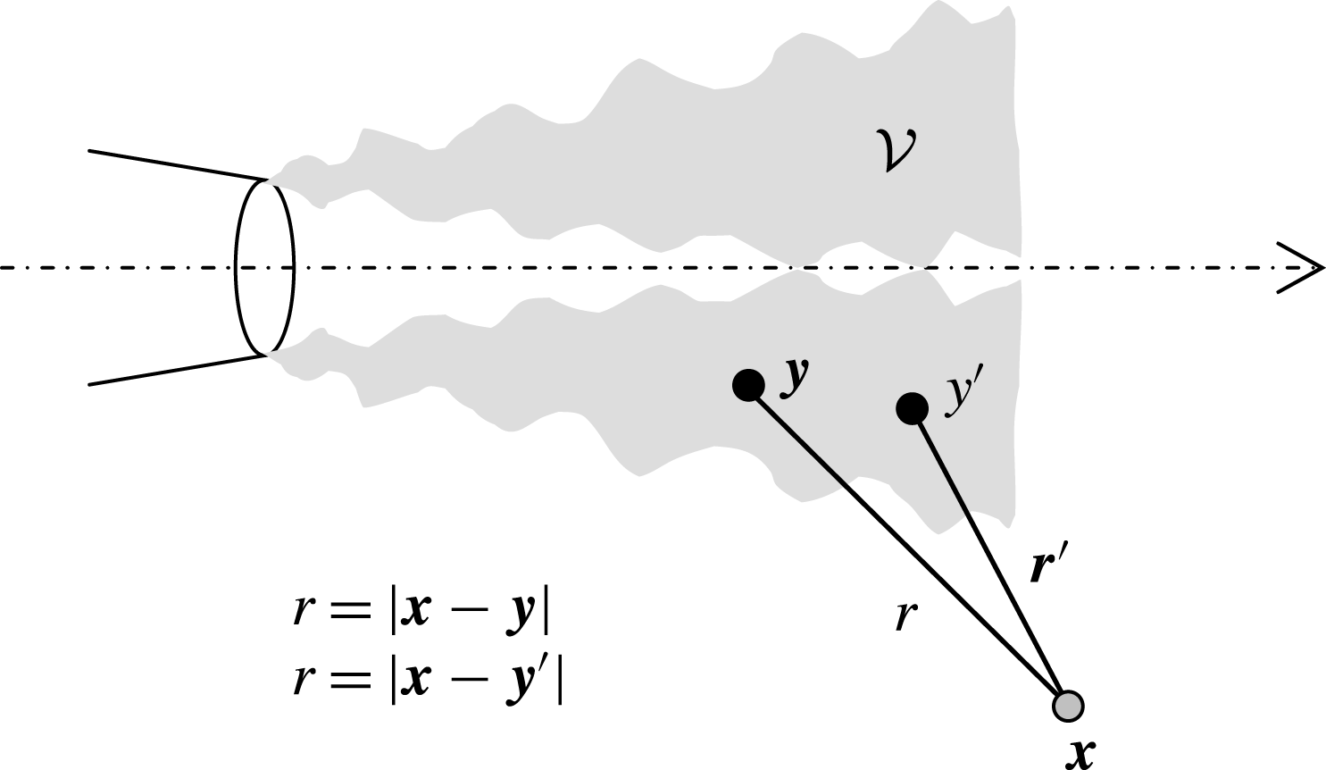
Figure 1. Set-up of the Lighthill acoustic analogy model.
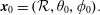
3.2 Spectral density
Using (3.4) the autocorrelation of the pressure at observer location
 $\boldsymbol{x}_{0}$
is
$\boldsymbol{x}_{0}$
is
 $$\begin{eqnarray}\displaystyle & & \displaystyle \overline{p^{\prime }(\boldsymbol{x}_{0},t)p^{\prime }(\boldsymbol{x}_{0},t+\unicode[STIX]{x1D70F})}=\frac{1}{16\unicode[STIX]{x03C0}^{2}a_{\infty }^{4}}\int _{{\mathcal{V}}}\int _{{\mathcal{V}}}[\unicode[STIX]{x1D717}_{i}\unicode[STIX]{x1D717}_{j}\unicode[STIX]{x1D717}_{k}^{\prime }\unicode[STIX]{x1D717}_{l}^{\prime }]_{0}\nonumber\\ \displaystyle & & \displaystyle \quad \times \,\overline{\frac{\unicode[STIX]{x2202}^{2}\unicode[STIX]{x1D61B}_{ij}(\boldsymbol{y},t-r_{0}/a_{\infty })}{\unicode[STIX]{x2202}t^{2}}\frac{\unicode[STIX]{x2202}^{2}\unicode[STIX]{x1D61B}_{kl}(\boldsymbol{y}^{\prime },t+\unicode[STIX]{x1D70F}-r_{0}^{\prime }/a_{\infty })}{\unicode[STIX]{x2202}t^{2}}}\frac{1}{r_{0}r_{0}^{\prime }}\,\text{d}^{3}\boldsymbol{y}^{\prime }\,\text{d}^{3}\boldsymbol{y}.\end{eqnarray}$$
Here
 $\overline{(\text{ })}$
denotes the expected value or ensemble average,
$\overline{(\text{ })}$
denotes the expected value or ensemble average,
 $r_{0}=|\boldsymbol{x}_{0}-\boldsymbol{y}|$
, and
$r_{0}=|\boldsymbol{x}_{0}-\boldsymbol{y}|$
, and
 $r_{0}^{\prime }=|\boldsymbol{x}_{0}-\boldsymbol{y}^{\prime }|$
. We assume stationarity in time and define accordingly the space–time correlation of the Lighthill stress tensor as
$r_{0}^{\prime }=|\boldsymbol{x}_{0}-\boldsymbol{y}^{\prime }|$
. We assume stationarity in time and define accordingly the space–time correlation of the Lighthill stress tensor as
 $$\begin{eqnarray}R_{ijkl}(\boldsymbol{y},\boldsymbol{y}^{\prime },\unicode[STIX]{x1D70F})=\overline{\unicode[STIX]{x1D61B}_{ij}(\boldsymbol{y},t)\unicode[STIX]{x1D61B}_{kl}(\boldsymbol{y}^{\prime },t+\unicode[STIX]{x1D70F})}.\end{eqnarray}$$
The stationarity allows us to take the time differentiation outside the correlation of (3.6), writing it as
 $\unicode[STIX]{x2202}^{4}/\unicode[STIX]{x2202}\unicode[STIX]{x1D70F}^{4}\overline{(\text{ })}$
(Papoulis Reference Papoulis1965). In addition, it enables the time shift
$\unicode[STIX]{x2202}^{4}/\unicode[STIX]{x2202}\unicode[STIX]{x1D70F}^{4}\overline{(\text{ })}$
(Papoulis Reference Papoulis1965). In addition, it enables the time shift
 $t-r_{0}/a_{\infty }\rightarrow t$
. These steps result in
$t-r_{0}/a_{\infty }\rightarrow t$
. These steps result in
 $$\begin{eqnarray}\displaystyle \overline{p^{\prime }(\boldsymbol{x}_{0},t)p^{\prime }(\boldsymbol{x}_{0},t+\unicode[STIX]{x1D70F})} & = & \displaystyle \frac{1}{16\unicode[STIX]{x03C0}^{2}a_{\infty }^{4}}\int _{{\mathcal{V}}}\int _{{\mathcal{V}}}[\unicode[STIX]{x1D717}_{i}\unicode[STIX]{x1D717}_{j}\unicode[STIX]{x1D717}_{k}^{\prime }\unicode[STIX]{x1D717}_{l}^{\prime }]_{0}\nonumber\\ \displaystyle & & \displaystyle \times \,\frac{\unicode[STIX]{x2202}^{4}}{\unicode[STIX]{x2202}\unicode[STIX]{x1D70F}^{4}}R_{ijkl}\left(\boldsymbol{y},\boldsymbol{y}^{\prime },\unicode[STIX]{x1D70F}+\frac{r_{0}-r_{0}^{\prime }}{a_{\infty }}\right)\frac{1}{r_{0}r_{0}^{\prime }}\,\text{d}^{3}\boldsymbol{y}^{\prime }\,\text{d}^{3}\boldsymbol{y}.\end{eqnarray}$$
The spectral density is the Fourier transform of the autocorrelation,
 $$\begin{eqnarray}S(\boldsymbol{x}_{0},\unicode[STIX]{x1D714})=\int _{-\infty }^{\infty }\overline{p^{\prime }(\boldsymbol{x}_{0},t)p^{\prime }(\boldsymbol{x}_{0},t+\unicode[STIX]{x1D70F})}\,\text{e}^{-\text{i}\unicode[STIX]{x1D714}\unicode[STIX]{x1D70F}}\,\text{d}\unicode[STIX]{x1D70F}.\end{eqnarray}$$
Inserting (3.8),
 $$\begin{eqnarray}S(\boldsymbol{x}_{0},\unicode[STIX]{x1D714})=\frac{\unicode[STIX]{x1D6FC}^{4}}{16\unicode[STIX]{x03C0}^{2}}\int _{{\mathcal{V}}}\int _{{\mathcal{V}}}\int _{-\infty }^{\infty }[\unicode[STIX]{x1D717}_{i}\unicode[STIX]{x1D717}_{j}\unicode[STIX]{x1D717}_{k}^{\prime }\unicode[STIX]{x1D717}_{l}^{\prime }]_{0}R_{ijkl}(\boldsymbol{y},\boldsymbol{y}^{\prime },\unicode[STIX]{x1D70F})\frac{\exp [\text{i}\unicode[STIX]{x1D6FC}(r_{0}-r_{0}^{\prime })-\text{i}\unicode[STIX]{x1D714}\unicode[STIX]{x1D70F}]}{r_{0}r_{0}^{\prime }}\,\text{d}\unicode[STIX]{x1D70F}\,\text{d}^{3}\boldsymbol{y}^{\prime }\,\text{d}^{3}\boldsymbol{y},\end{eqnarray}$$
where
 $\unicode[STIX]{x1D6FC}=\unicode[STIX]{x1D714}/a_{\infty }$
is the acoustic wavenumber. Equation (3.10) gives the acoustic component of the spectral density everywhere. At this point the only assumption is the stationarity in time of the flow statistics.
$\unicode[STIX]{x1D6FC}=\unicode[STIX]{x1D714}/a_{\infty }$
is the acoustic wavenumber. Equation (3.10) gives the acoustic component of the spectral density everywhere. At this point the only assumption is the stationarity in time of the flow statistics.
3.3 Coordinate system
The study of azimuthal effects necessitates the use of a cylindrical polar coordinate system in the implementation of (3.10). The complexity of the problem requires the inclusion of Cartesian and spherical coordinates. The three coordinate systems used here are illustrated in figure 2: Cartesian
 $(X,Y,Z)$
; cylindrical polar
$(X,Y,Z)$
; cylindrical polar
 $(X,y,\unicode[STIX]{x1D719})$
; and spherical
$(X,y,\unicode[STIX]{x1D719})$
; and spherical
 $({\mathcal{R}},\unicode[STIX]{x1D703},\unicode[STIX]{x1D719})$
. The Cartesian coordinate system will also be described by indices 1 (
$({\mathcal{R}},\unicode[STIX]{x1D703},\unicode[STIX]{x1D719})$
. The Cartesian coordinate system will also be described by indices 1 (
 $X$
), 2 (
$X$
), 2 (
 $Y$
) and 3 (
$Y$
) and 3 (
 $Z$
), with the index
$Z$
), with the index
 $23$
referring to combined properties on the cross-stream (
$23$
referring to combined properties on the cross-stream (
 $Y{-}Z$
) plane. Index 4 will refer to time.
$Y{-}Z$
) plane. Index 4 will refer to time.
Selection of an appropriate jet axis, on which the definitions of radial distance
 $y$
and azimuthal angle
$y$
and azimuthal angle
 $\unicode[STIX]{x1D719}$
are based, is critical for capturing the azimuthal effects on noise emission. In this regard, the nozzle axis is a poor choice because asymmetric jets have distorted mean velocity profiles and could be vectored in directions off the nozzle axis. In § 3.6 the Lighthill stress tensor will be connected to the Reynolds stress, whose dominant component scales with the magnitude of the mean velocity gradient
$\unicode[STIX]{x1D719}$
are based, is critical for capturing the azimuthal effects on noise emission. In this regard, the nozzle axis is a poor choice because asymmetric jets have distorted mean velocity profiles and could be vectored in directions off the nozzle axis. In § 3.6 the Lighthill stress tensor will be connected to the Reynolds stress, whose dominant component scales with the magnitude of the mean velocity gradient
 $$\begin{eqnarray}G=|\unicode[STIX]{x1D735}\overline{\boldsymbol{u}}|.\end{eqnarray}$$
The decision then is to define the centre of the jet as the point where the Reynolds stress vanishes, or
 $G=0$
, within the jet flow. This definition is straightforward for the region past the end of the primary potential core, where the profile of the mean flow is Gaussian-like. There, the location of
$G=0$
, within the jet flow. This definition is straightforward for the region past the end of the primary potential core, where the profile of the mean flow is Gaussian-like. There, the location of
 $G=0$
coincides with the location of the maximum mean velocity
$G=0$
coincides with the location of the maximum mean velocity
 $\overline{u}_{max}$
. For the region of the jet comprising the primary potential core, the locations of
$\overline{u}_{max}$
. For the region of the jet comprising the primary potential core, the locations of
 $G=0$
or
$G=0$
or
 $\overline{u}_{max}$
are ill defined. However, one can calculate fairly reliably the centroid of the high-speed region defined by a criterion like
$\overline{u}_{max}$
are ill defined. However, one can calculate fairly reliably the centroid of the high-speed region defined by a criterion like
 $\overline{u}>0.9\overline{u}_{max}$
. In fact, this criterion can be extended to the region past the end of the primary potential core where, for noisy experimental or numerical data, it provides a more reliable estimate of the location of
$\overline{u}>0.9\overline{u}_{max}$
. In fact, this criterion can be extended to the region past the end of the primary potential core where, for noisy experimental or numerical data, it provides a more reliable estimate of the location of
 $\overline{u}_{max}$
. Therefore, for a given axial station
$\overline{u}_{max}$
. Therefore, for a given axial station
 $X=X_{1}$
, we identify the region of high-speed flow using the criterion
$X=X_{1}$
, we identify the region of high-speed flow using the criterion
 $$\begin{eqnarray}\overline{u}(X_{1},Y,Z)>0.9\overline{u}_{max}(X_{1}).\end{eqnarray}$$
Considering a flow with symmetry about the
 $X{-}Y$
plane, we denote
$X{-}Y$
plane, we denote
 $Y_{i}$
,
$Y_{i}$
,
 $i=1,\ldots ,N$
, the
$i=1,\ldots ,N$
, the
 $Y$
locations at which this criterion is satisfied. Then, the jet centroid is computed according to
$Y$
locations at which this criterion is satisfied. Then, the jet centroid is computed according to
 $$\begin{eqnarray}Y_{c}(X_{1})=\frac{1}{N}\mathop{\sum }_{i=1}^{N}Y_{i}.\end{eqnarray}$$
Subsequently, the
 $Y$
-coordinates of all the data points at this axial station are decremented by
$Y$
-coordinates of all the data points at this axial station are decremented by
 $Y_{c}$
, so that
$Y_{c}$
, so that
 $Y=0$
becomes the centroid location. This process is applied to all the axial stations within the computational domain.
$Y=0$
becomes the centroid location. This process is applied to all the axial stations within the computational domain.
Figure 2. Coordinate systems.
3.4 Far-field approximation
The far-field version of (3.10) is now developed, using the coordinate systems depicted in figure 2. The source locations are described in cylindrical polar coordinates
 $$\begin{eqnarray}\boldsymbol{y}=(X,y,\unicode[STIX]{x1D719}),\quad \boldsymbol{y}^{\prime }=(X^{\prime },y^{\prime },\unicode[STIX]{x1D719}^{\prime }).\end{eqnarray}$$
In the spherical coordinate system, the observer is situated at
 $$\begin{eqnarray}\boldsymbol{x}_{0}=({\mathcal{R}},\unicode[STIX]{x1D703}_{0},\unicode[STIX]{x1D719}_{0}).\end{eqnarray}$$
For
 ${\mathcal{R}}\gg \ell$
, where
${\mathcal{R}}\gg \ell$
, where
 $\ell$
is a characteristic dimension of the source,
$\ell$
is a characteristic dimension of the source,
 $\unicode[STIX]{x1D717}_{i}\approx \unicode[STIX]{x1D717}_{i}^{\prime }\approx x_{i}/{\mathcal{R}}$
and
$\unicode[STIX]{x1D717}_{i}\approx \unicode[STIX]{x1D717}_{i}^{\prime }\approx x_{i}/{\mathcal{R}}$
and
 $1/(r_{0}r_{0}^{\prime })\approx 1/{\mathcal{R}}^{2}$
. Further,
$1/(r_{0}r_{0}^{\prime })\approx 1/{\mathcal{R}}^{2}$
. Further,
 $$\begin{eqnarray}r_{0}-r_{0}^{\prime }\approx (X^{\prime }{-}X)\cos \unicode[STIX]{x1D703}_{0}+\sin \unicode[STIX]{x1D703}_{0}[y^{\prime }\cos (\unicode[STIX]{x1D719}^{\prime }-\unicode[STIX]{x1D719}_{0})-y\cos (\unicode[STIX]{x1D719}-\unicode[STIX]{x1D719}_{0})].\end{eqnarray}$$
Although the axial source separation
 $X^{\prime }{-}X$
readily appears on the right-hand side, the radial and azimuthal separations are interconnected and cannot be separated cleanly into distinct terms. This is an important consequence of using the polar-cylindrical coordinate system to express the source location; it will prevent the formulation of the spectral density as a four-dimensional Fourier transform of the space–time correlation, a common procedure in past treatments of the acoustic analogy (Morris & Farassat Reference Morris and Farassat2002; Dowling & Hynes Reference Dowling and Hynes2004).
$X^{\prime }{-}X$
readily appears on the right-hand side, the radial and azimuthal separations are interconnected and cannot be separated cleanly into distinct terms. This is an important consequence of using the polar-cylindrical coordinate system to express the source location; it will prevent the formulation of the spectral density as a four-dimensional Fourier transform of the space–time correlation, a common procedure in past treatments of the acoustic analogy (Morris & Farassat Reference Morris and Farassat2002; Dowling & Hynes Reference Dowling and Hynes2004).
On defining the projection of
 $R_{ijkl}$
along the observer direction as
$R_{ijkl}$
along the observer direction as
 $$\begin{eqnarray}R_{0000}(\boldsymbol{y},\boldsymbol{y}^{\prime },\unicode[STIX]{x1D70F})=[\unicode[STIX]{x1D717}_{i}\unicode[STIX]{x1D717}_{j}~\unicode[STIX]{x1D717}_{k}\unicode[STIX]{x1D717}_{l}]_{0}~R_{ijkl}(\boldsymbol{y},\boldsymbol{y}^{\prime },\unicode[STIX]{x1D70F})\end{eqnarray}$$
the spectral density for the far-field observer becomes
 $$\begin{eqnarray}\displaystyle & & \displaystyle S(\boldsymbol{x}_{0},\unicode[STIX]{x1D714})=\frac{\unicode[STIX]{x1D6FC}^{4}}{16\unicode[STIX]{x03C0}^{2}{\mathcal{R}}^{2}}\int _{{\mathcal{V}}}\int _{-\unicode[STIX]{x03C0}}^{\unicode[STIX]{x03C0}}\int _{0}^{\infty }\int _{0}^{\infty }\int _{-\infty }^{\infty }R_{0000}(\boldsymbol{y},\boldsymbol{y}^{\prime },\unicode[STIX]{x1D70F})\nonumber\\ \displaystyle & & \displaystyle \quad \times \,\exp (\text{i}\unicode[STIX]{x1D6FC}\cos \unicode[STIX]{x1D703}_{0}(X^{\prime }{-}X)-\text{i}\unicode[STIX]{x1D714}\unicode[STIX]{x1D70F})\nonumber\\ \displaystyle & & \displaystyle \quad \times \,\exp \{\text{i}\unicode[STIX]{x1D6FC}\sin \unicode[STIX]{x1D703}_{0}[y^{\prime }\cos (\unicode[STIX]{x1D719}^{\prime }-\unicode[STIX]{x1D719}_{0})-y\cos (\unicode[STIX]{x1D719}-\unicode[STIX]{x1D719}_{0})]\}\,\text{d}\unicode[STIX]{x1D70F}\,\text{d}X^{\prime }y^{\prime }\,\text{d}y^{\prime }\,\text{d}\unicode[STIX]{x1D719}^{\prime }\,\text{d}^{3}\boldsymbol{y}.\qquad\end{eqnarray}$$
In (3.18) the integrals over the shifted space and time coordinates are shown explicitly, while the integration over the source volume
 ${\mathcal{V}}$
is displayed compactly. The spatial coordinates in the exponent arise from the free-space Green’s function in the frequency domain.
${\mathcal{V}}$
is displayed compactly. The spatial coordinates in the exponent arise from the free-space Green’s function in the frequency domain.
3.5 Model for the space–time correlation
The space–time correlation model used here is defined in a fixed frame of reference. It is guided by experimental measurements of space–time correlations in the flow or near acoustic field of turbulent jets (Harper-Bourne Reference Harper-Bourne2003; Doty & McLaughlin Reference Doty and McLaughlin2005; Morris & Zaman Reference Morris and Zaman2010b
; Viswanathan et al.
Reference Viswanathan, Underbrink and Brusniak2011), with important simplifications and modifications. Figure 3 sketches the typical shape of the axial space–time correlation of a fluctuating quantity (velocity, velocity squared, pressure, etc.). The evolution of the timewise correlation
 $R_{4}$
reflects the convection of turbulence with a velocity
$R_{4}$
reflects the convection of turbulence with a velocity
 $U_{c}$
and its decorrelation with increasing axial separation
$U_{c}$
and its decorrelation with increasing axial separation
 $|X^{\prime }{-}X|$
. At zero spatial separation,
$|X^{\prime }{-}X|$
. At zero spatial separation,
 $R_{4}$
is the autocorrelation and decays approximately exponentially with the time separation
$R_{4}$
is the autocorrelation and decays approximately exponentially with the time separation
 $\unicode[STIX]{x1D70F}$
. With increasing
$\unicode[STIX]{x1D70F}$
. With increasing
 $|X^{\prime }{-}X|$
, the timewise correlation peaks at
$|X^{\prime }{-}X|$
, the timewise correlation peaks at
 $\unicode[STIX]{x1D70F}=(X^{\prime }{-}X)/U_{c}$
and is modulated by the axial correlation
$\unicode[STIX]{x1D70F}=(X^{\prime }{-}X)/U_{c}$
and is modulated by the axial correlation
 $R_{1}(X^{\prime }{-}X)$
; in addition, the shape of
$R_{1}(X^{\prime }{-}X)$
; in addition, the shape of
 $R_{4}$
broadens and becomes more Gaussian-like. Negative loops are evident throughout the evolution of
$R_{4}$
broadens and becomes more Gaussian-like. Negative loops are evident throughout the evolution of
 $R_{4}$
. For finite axial separation, the space–time correlation is not symmetric around
$R_{4}$
. For finite axial separation, the space–time correlation is not symmetric around
 $\unicode[STIX]{x1D70F}=0$
, reflecting the non-stationarity of spatial statistics and the associated increase of length and time scales with downstream distance.
$\unicode[STIX]{x1D70F}=0$
, reflecting the non-stationarity of spatial statistics and the associated increase of length and time scales with downstream distance.

Figure 3. Illustration of the typical shape of the axial space–time correlation.
Having noted the principal features of the axial space–time correlation, we outline the simplifications and modifications implemented here. The timewise and axial correlations will be treated as symmetric functions, thus neglecting the effects of spatial non-stationarity on their distributions. The timewise correlation
 $R_{4}$
will have fixed shape with axial separation and will include a transverse propagation time, in addition to the axial propagation time noted above. In the transverse dimensions of the problem, we will employ a mixed correlation
$R_{4}$
will have fixed shape with axial separation and will include a transverse propagation time, in addition to the axial propagation time noted above. In the transverse dimensions of the problem, we will employ a mixed correlation
 $R_{23}$
whose precise form will be the subject of detailed analysis. The resulting correlation has the form
$R_{23}$
whose precise form will be the subject of detailed analysis. The resulting correlation has the form
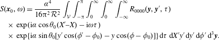
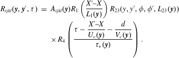 $$\begin{eqnarray}\displaystyle R_{ijkl}(\boldsymbol{y},\boldsymbol{y}^{\prime },\unicode[STIX]{x1D70F}) & = & \displaystyle A_{ijkl}(\boldsymbol{y})R_{1}\left(\frac{X^{\prime }{-}X}{L_{1}(\boldsymbol{y})}\right)R_{23}(y,y^{\prime },\unicode[STIX]{x1D719},\unicode[STIX]{x1D719}^{\prime },L_{23}(\boldsymbol{y}))\nonumber\\ \displaystyle & & \displaystyle \times \,R_{4}\left({\displaystyle \frac{\unicode[STIX]{x1D70F}-\displaystyle {\displaystyle \frac{X^{\prime }{-}X}{U_{c}(\boldsymbol{y})}}-{\displaystyle \frac{d}{V_{c}(\boldsymbol{y})}}}{\unicode[STIX]{x1D70F}_{\ast }(\boldsymbol{y})}}\right).\end{eqnarray}$$
Here
 $A_{ijkl}$
is the amplitude of the correlation;
$A_{ijkl}$
is the amplitude of the correlation;
 $R_{1}$
and
$R_{1}$
and
 $R_{4}$
are the axial and timewise correlations, respectively;
$R_{4}$
are the axial and timewise correlations, respectively;
 $R_{23}$
is a mixed radial/azimuthal correlation;
$R_{23}$
is a mixed radial/azimuthal correlation;
 $L_{1}$
and
$L_{1}$
and
 $L_{23}$
and are the correlation length scales in the axial and transverse directions, respectively; and
$L_{23}$
and are the correlation length scales in the axial and transverse directions, respectively; and
 $\unicode[STIX]{x1D70F}_{\ast }$
is the correlation time scale. The timewise correlation
$\unicode[STIX]{x1D70F}_{\ast }$
is the correlation time scale. The timewise correlation
 $R_{4}$
includes axial and transverse propagation times. The axial propagation time
$R_{4}$
includes axial and transverse propagation times. The axial propagation time
 $(X^{\prime }{-}X)/U_{c}$
is connected to the streamwise eddy convection at velocity
$(X^{\prime }{-}X)/U_{c}$
is connected to the streamwise eddy convection at velocity
 $U_{c}$
. The transverse propagation time
$U_{c}$
. The transverse propagation time
 $d/V_{c}$
is a special construct that will be shown to induce azimuthal directivity in the emission of the sound. It is based on a transverse distance
$d/V_{c}$
is a special construct that will be shown to induce azimuthal directivity in the emission of the sound. It is based on a transverse distance
 $d$
and a transverse propagation velocity
$d$
and a transverse propagation velocity
 $V_{c}$
. The axial and transverse convective Mach numbers are
$V_{c}$
. The axial and transverse convective Mach numbers are
 $M_{c}=U_{c}/a_{\infty }$
and
$M_{c}=U_{c}/a_{\infty }$
and
 $\unicode[STIX]{x1D707}_{c}=V_{c}/a_{\infty }$
, respectively. Equation (3.19) shows explicitly the dependence of the amplitude and correlation scales on the source location
$\unicode[STIX]{x1D707}_{c}=V_{c}/a_{\infty }$
, respectively. Equation (3.19) shows explicitly the dependence of the amplitude and correlation scales on the source location
 $\boldsymbol{y}$
. This notation will be henceforth dropped to reduce clutter.
$\boldsymbol{y}$
. This notation will be henceforth dropped to reduce clutter.
The notion of a transverse propagation time scale can be found in the works of Harper-Bourne (Reference Harper-Bourne2003), Raizada & Morris (Reference Raizada and Morris2006) and Miller (Reference Miller2014). In this study, the concept should not be seen as anything more than a mathematical construct to induce azimuthal influence, as will be demonstrated in the analysis of § 3.5.3. Nevertheless, it is helpful to have some insight as to the physical meaning of
 $V_{c}$
. Consider two points separated laterally at the same axial location. If the turbulence is highly uncorrelated spatially, so that the correlation scale is much smaller than the separation of the two points, the speed at which a disturbance propagates from the first point to the second point cannot exceed the local acoustic velocity. On the other hand, if the turbulence convects downstream in highly organized patterns whose correlation scale is much larger than the separation of the two points, then the lateral propagation speed depends on the axial convective velocity and the shape of the ‘wavefronts’. If a given wavefront arrives simultaneously at the two points, the lateral propagation speed is infinite. Experimental measurements of the second-order radial cross-correlation in subsonic jets by Morris & Zaman (Reference Morris and Zaman2010a
) suggest a very fast, yet finite, lateral convection velocity. In the uncorrelated case, a transverse convective Mach number of the order of 1 (
$V_{c}$
. Consider two points separated laterally at the same axial location. If the turbulence is highly uncorrelated spatially, so that the correlation scale is much smaller than the separation of the two points, the speed at which a disturbance propagates from the first point to the second point cannot exceed the local acoustic velocity. On the other hand, if the turbulence convects downstream in highly organized patterns whose correlation scale is much larger than the separation of the two points, then the lateral propagation speed depends on the axial convective velocity and the shape of the ‘wavefronts’. If a given wavefront arrives simultaneously at the two points, the lateral propagation speed is infinite. Experimental measurements of the second-order radial cross-correlation in subsonic jets by Morris & Zaman (Reference Morris and Zaman2010a
) suggest a very fast, yet finite, lateral convection velocity. In the uncorrelated case, a transverse convective Mach number of the order of 1 (
 $\unicode[STIX]{x1D707}_{c}\sim 1$
) represents an upper bound. In the strongly correlated case,
$\unicode[STIX]{x1D707}_{c}\sim 1$
) represents an upper bound. In the strongly correlated case,
 $\unicode[STIX]{x1D707}_{c}$
can be as high as
$\unicode[STIX]{x1D707}_{c}$
can be as high as
 $\infty$
in which case the transverse term drops out from the argument of
$\infty$
in which case the transverse term drops out from the argument of
 $R_{4}$
.
$R_{4}$
.
3.5.1 Generic shape for the correlations
The correlation shapes employed here fall under the class of the ‘stretched exponential’
 $$\begin{eqnarray}R_{j}(t)=\text{e}^{-|t|^{\unicode[STIX]{x1D6FD}_{j}}},\end{eqnarray}$$
also called the Kohlrausch function (Wuttke Reference Wuttke2012). The flexibility provided by this function will be used in the axial (
 $j=1$
) and timewise (
$j=1$
) and timewise (
 $j=4$
) dimensions, where the range
$j=4$
) dimensions, where the range
 $0.7\leqslant \unicode[STIX]{x1D6FD}_{j}\leqslant 2$
will be allowed. On the transverse plane (
$0.7\leqslant \unicode[STIX]{x1D6FD}_{j}\leqslant 2$
will be allowed. On the transverse plane (
 $j=23$
) only the integer value
$j=23$
) only the integer value
 $\unicode[STIX]{x1D6FD}_{23}=2$
will be considered for the sake of numerical efficiency.
$\unicode[STIX]{x1D6FD}_{23}=2$
will be considered for the sake of numerical efficiency.
Since
 $R_{j}$
is an even function, its Fourier transform is real and equal to twice the cosine transform:
$R_{j}$
is an even function, its Fourier transform is real and equal to twice the cosine transform:
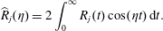 $$\begin{eqnarray}\widehat{R}_{j}(\unicode[STIX]{x1D702})=2\int _{0}^{\infty }R_{j}(t)\cos (\unicode[STIX]{x1D702}t)\,\text{d}t.\end{eqnarray}$$
Note that
 $\widehat{R}_{j}$
assumes the analytical forms
$\widehat{R}_{j}$
assumes the analytical forms
 $$\begin{eqnarray}\left.\begin{array}{@{}c@{}}\displaystyle \widehat{R}_{j}(\unicode[STIX]{x1D702})=\frac{2}{1+\unicode[STIX]{x1D702}^{2}},\quad \unicode[STIX]{x1D6FD}_{j}=1\\ \displaystyle \widehat{R}_{j}(\unicode[STIX]{x1D702})=\sqrt{\unicode[STIX]{x03C0}}\text{e}^{-(1/4)\unicode[STIX]{x1D702}^{2}},\quad \unicode[STIX]{x1D6FD}_{j}=2.\end{array}\right\}\end{eqnarray}$$
For powers
 $\unicode[STIX]{x1D6FD}_{j}$
other than 1 (exponential) or 2 (Gaussian) the Fourier transform does not have an analytical expression and needs to be calculated numerically. For computational efficiency, the transform
$\unicode[STIX]{x1D6FD}_{j}$
other than 1 (exponential) or 2 (Gaussian) the Fourier transform does not have an analytical expression and needs to be calculated numerically. For computational efficiency, the transform
 $\widehat{R}_{j}(\unicode[STIX]{x1D702})$
was computed once and was tabulated versus
$\widehat{R}_{j}(\unicode[STIX]{x1D702})$
was computed once and was tabulated versus
 $\unicode[STIX]{x1D702}$
and
$\unicode[STIX]{x1D702}$
and
 $\unicode[STIX]{x1D6FD}_{j}$
; subsequent operations used two-dimensional interpolation of the table. Great care is required in evaluating near
$\unicode[STIX]{x1D6FD}_{j}$
; subsequent operations used two-dimensional interpolation of the table. Great care is required in evaluating near
 $\unicode[STIX]{x1D6FD}_{j}=2$
where the shape of the Fourier transform is extremely sensitive on
$\unicode[STIX]{x1D6FD}_{j}=2$
where the shape of the Fourier transform is extremely sensitive on
 $2-\unicode[STIX]{x1D6FD}_{j}$
.
$2-\unicode[STIX]{x1D6FD}_{j}$
.
The stretched exponential will be used here with a reference scale, that is,
 $R_{j}(t)=\exp (-|t/\unicode[STIX]{x1D70F}|^{\unicode[STIX]{x1D6FD}_{j}})$
. Its Fourier transform is simply
$R_{j}(t)=\exp (-|t/\unicode[STIX]{x1D70F}|^{\unicode[STIX]{x1D6FD}_{j}})$
. Its Fourier transform is simply
 $\unicode[STIX]{x1D70F}\widehat{R}_{j}(\unicode[STIX]{x1D70F}\unicode[STIX]{x1D702})$
. Evaluated at
$\unicode[STIX]{x1D70F}\widehat{R}_{j}(\unicode[STIX]{x1D70F}\unicode[STIX]{x1D702})$
. Evaluated at
 $\unicode[STIX]{x1D702}=0$
, it gives the integral scale
$\unicode[STIX]{x1D702}=0$
, it gives the integral scale
 $\unicode[STIX]{x1D70F}\widehat{R}_{j}(0)$
. It can be shown that
$\unicode[STIX]{x1D70F}\widehat{R}_{j}(0)$
. It can be shown that
 $$\begin{eqnarray}\widehat{R}_{j}(0)=\frac{1}{\unicode[STIX]{x1D6FD}_{j}}\unicode[STIX]{x1D6E4}\left(\frac{1}{\unicode[STIX]{x1D6FD}_{j}}\right),\end{eqnarray}$$
where
 $\unicode[STIX]{x1D6E4}$
is the gamma function (Wuttke Reference Wuttke2012). For
$\unicode[STIX]{x1D6E4}$
is the gamma function (Wuttke Reference Wuttke2012). For
 $0.7\leqslant \unicode[STIX]{x1D6FD}_{j}\leqslant 2$
, the corresponding range for
$0.7\leqslant \unicode[STIX]{x1D6FD}_{j}\leqslant 2$
, the corresponding range for
 $\widehat{R}_{j}(0)$
is
$\widehat{R}_{j}(0)$
is
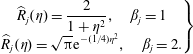
 $1.266\geqslant \widehat{R}_{j}(0)\geqslant 0.886$
. Thus, the integral scale is not too different from the reference scale.
$1.266\geqslant \widehat{R}_{j}(0)\geqslant 0.886$
. Thus, the integral scale is not too different from the reference scale.
Figure 4 illustrates the behaviour of the stretched exponential and its transform for
 $0.7\leqslant \unicode[STIX]{x1D6FD}_{j}\leqslant 2$
, the range allowed in this study. For clarity the transform is shown in decibels. The sensitivity of the transform on the power
$0.7\leqslant \unicode[STIX]{x1D6FD}_{j}\leqslant 2$
, the range allowed in this study. For clarity the transform is shown in decibels. The sensitivity of the transform on the power
 $\unicode[STIX]{x1D6FD}$
is apparent and represents a key ingredient of the optimization process employed here. For the selected range of
$\unicode[STIX]{x1D6FD}$
is apparent and represents a key ingredient of the optimization process employed here. For the selected range of
 $\unicode[STIX]{x1D6FD}_{j}$
, the Fourier transform is non-negative for all frequencies.
$\unicode[STIX]{x1D6FD}_{j}$
, the Fourier transform is non-negative for all frequencies.
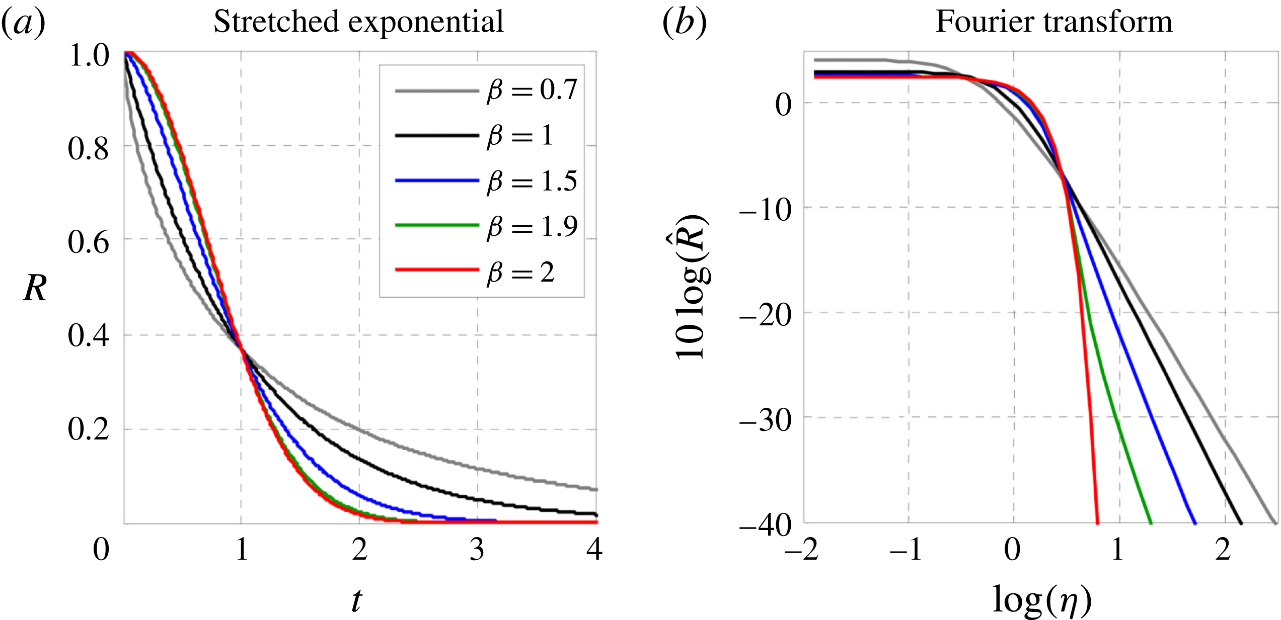
Figure 4. Correlation function (a) and its Fourier transformation (b) for various values of
 $\unicode[STIX]{x1D6FD}$
.
$\unicode[STIX]{x1D6FD}$
.
3.5.2 Axial and timewise Fourier transforms
The timewise integration in (3.18) amounts to a Fourier transform in the time separation
 $\unicode[STIX]{x1D70F}$
. Given the slow axial development of the flow, the
$\unicode[STIX]{x1D70F}$
. Given the slow axial development of the flow, the
 $X^{\prime }$
integral can be approximated as an integral over the axial separation
$X^{\prime }$
integral can be approximated as an integral over the axial separation
 $X^{\prime }{-}X$
ranging from
$X^{\prime }{-}X$
ranging from
 $-\infty$
to
$-\infty$
to
 $\infty$
, and thus can also be treated as a Fourier transform in
$\infty$
, and thus can also be treated as a Fourier transform in
 $X^{\prime }{-}X$
. This assumes that the scale of the axial correlation is much smaller than the distances
$X^{\prime }{-}X$
. This assumes that the scale of the axial correlation is much smaller than the distances
 $X$
or
$X$
or
 $X^{\prime }$
and neglects the fact that
$X^{\prime }$
and neglects the fact that
 $X$
and
$X$
and
 $X^{\prime }$
have a finite origin at zero. Fourier transforms in the transverse dimensions of the problem are not feasible or appropriate. As indicated in the discussion of (3.16), the radial and azimuthal components of the Green’s function cannot be expressed in terms of separations
$X^{\prime }$
have a finite origin at zero. Fourier transforms in the transverse dimensions of the problem are not feasible or appropriate. As indicated in the discussion of (3.16), the radial and azimuthal components of the Green’s function cannot be expressed in terms of separations
 $y^{\prime }-y$
and
$y^{\prime }-y$
and
 $\unicode[STIX]{x1D719}^{\prime }-\unicode[STIX]{x1D719}$
. Even if one were to overlook this fact, the concept of a Fourier transform in the radial separation
$\unicode[STIX]{x1D719}^{\prime }-\unicode[STIX]{x1D719}$
. Even if one were to overlook this fact, the concept of a Fourier transform in the radial separation
 $y^{\prime }-y$
breaks down because of the rapid evolution of the flow in the radial direction: the radial correlation scale cannot be considered small compared to either
$y^{\prime }-y$
breaks down because of the rapid evolution of the flow in the radial direction: the radial correlation scale cannot be considered small compared to either
 $y^{\prime }$
or
$y^{\prime }$
or
 $y$
. Similarly, the azimuthal correlation scale is not necessarily small compared to
$y$
. Similarly, the azimuthal correlation scale is not necessarily small compared to
 $2\unicode[STIX]{x03C0}$
to attempt a Fourier transform in
$2\unicode[STIX]{x03C0}$
to attempt a Fourier transform in
 $\unicode[STIX]{x1D719}^{\prime }$
.
$\unicode[STIX]{x1D719}^{\prime }$
.
We conclude that Fourier transformation is only possible in the timewise and axial directions; the procedure is rigorous in the timewise dimension and acceptable as an approximation in the axial dimension. Inserting the correlation form (3.19) in (3.18), and carrying out the Fourier transforms in
 $\unicode[STIX]{x1D70F}$
and
$\unicode[STIX]{x1D70F}$
and
 $X^{\prime }{-}X$
, we obtain
$X^{\prime }{-}X$
, we obtain
 $$\begin{eqnarray}\displaystyle & & \displaystyle S(\boldsymbol{x}_{0},\unicode[STIX]{x1D714})=\frac{\unicode[STIX]{x1D6FC}^{4}}{16\unicode[STIX]{x03C0}^{2}{\mathcal{R}}^{2}}\int _{{\mathcal{V}}}A_{0000}\unicode[STIX]{x1D70F}_{\ast }L_{1}\widehat{R}_{1}\left[\unicode[STIX]{x1D6FC}L_{1}\left(\frac{1}{M_{c}}-\cos \unicode[STIX]{x1D703}_{0}\right)\right]\widehat{R}_{4}[\unicode[STIX]{x1D714}\unicode[STIX]{x1D70F}_{\ast }]\exp \left(-\text{i}\frac{\unicode[STIX]{x1D6FC}d}{\unicode[STIX]{x1D707}_{c}}\right)\qquad \nonumber\\ \displaystyle & & \displaystyle \quad \times \,\int _{-\unicode[STIX]{x03C0}}^{\unicode[STIX]{x03C0}}\int _{0}^{\infty }R_{23}\exp \{\text{i}\unicode[STIX]{x1D6FC}\sin \unicode[STIX]{x1D703}_{0}[y^{\prime }\cos (\unicode[STIX]{x1D719}^{\prime }-\unicode[STIX]{x1D719}_{0})-y\cos (\unicode[STIX]{x1D719}-\unicode[STIX]{x1D719}_{0})]\}y^{\prime }\,\text{d}y^{\prime }\,\text{d}\unicode[STIX]{x1D719}^{\prime }\,\text{d}^{3}\boldsymbol{y}.\end{eqnarray}$$
Omitting the arguments, we write this compactly as
 $$\begin{eqnarray}S(\boldsymbol{x}_{0},\unicode[STIX]{x1D714})=\frac{\unicode[STIX]{x1D6FC}^{4}}{16\unicode[STIX]{x03C0}^{2}{\mathcal{R}}^{2}}\int _{{\mathcal{V}}}A_{0000}\unicode[STIX]{x1D70F}_{\ast }L_{1}\unicode[STIX]{x03C0}L_{23}^{2}\widehat{R}_{1}\widehat{R}_{4}\widetilde{R}_{23}\,\text{d}^{3}\boldsymbol{y},\end{eqnarray}$$
where
 $$\begin{eqnarray}\displaystyle \widetilde{R}_{23} & = & \displaystyle \frac{1}{\unicode[STIX]{x03C0}L_{23}^{2}}\int _{-\unicode[STIX]{x03C0}}^{\unicode[STIX]{x03C0}}\int _{0}^{\infty }R_{23}(y,y^{\prime },\unicode[STIX]{x1D719},\unicode[STIX]{x1D719}^{\prime })\nonumber\\ \displaystyle & & \displaystyle \times \,\exp \left\{\text{i}\unicode[STIX]{x1D6FC}\sin \unicode[STIX]{x1D703}_{0}[y^{\prime }\cos (\unicode[STIX]{x1D719}^{\prime }-\unicode[STIX]{x1D719}_{0})-y\cos (\unicode[STIX]{x1D719}-\unicode[STIX]{x1D719}_{0})]-\text{i}\unicode[STIX]{x1D6FC}\frac{d}{\unicode[STIX]{x1D707}_{c}}\right\}y^{\prime }\,\text{d}y^{\prime }\,\text{d}\unicode[STIX]{x1D719}^{\prime }.\qquad\end{eqnarray}$$
In (3.25) the term
 $\unicode[STIX]{x03C0}L_{23}^{2}$
represents a cross-stream correlation area, and the product
$\unicode[STIX]{x03C0}L_{23}^{2}$
represents a cross-stream correlation area, and the product
 $\unicode[STIX]{x1D70F}_{\ast }L_{1}\unicode[STIX]{x03C0}L_{23}^{2}$
can be viewed as a four-dimensional correlation ‘volume’. As discussed in § 3.5.1, the functions
$\unicode[STIX]{x1D70F}_{\ast }L_{1}\unicode[STIX]{x03C0}L_{23}^{2}$
can be viewed as a four-dimensional correlation ‘volume’. As discussed in § 3.5.1, the functions
 $\widehat{R}_{1}$
and
$\widehat{R}_{1}$
and
 $\widehat{R}_{4}$
are real and non-negative. The meaning and behaviour of
$\widehat{R}_{4}$
are real and non-negative. The meaning and behaviour of
 $\widetilde{R}_{23}$
will be the topic of the discussion that follows.
$\widetilde{R}_{23}$
will be the topic of the discussion that follows.
3.5.3 Cross-stream correlation
As noted in § 3.5.2, the transverse correlation
 $R_{23}$
is not amenable to Fourier transforms. Instead, the spectral transformation of
$R_{23}$
is not amenable to Fourier transforms. Instead, the spectral transformation of
 $R_{23}$
takes the form of the integral of (3.26). Evaluation of this integral, and determination of allowable forms for
$R_{23}$
takes the form of the integral of (3.26). Evaluation of this integral, and determination of allowable forms for
 $R_{23}$
and the separation distance
$R_{23}$
and the separation distance
 $d$
, are governed by the requirement that the power spectral density
$d$
, are governed by the requirement that the power spectral density
 $S(\boldsymbol{x}_{0},\unicode[STIX]{x1D714})$
, given by (3.25), be real and non-negative. To satisfy this requirement for an arbitrary source distribution,
$S(\boldsymbol{x}_{0},\unicode[STIX]{x1D714})$
, given by (3.25), be real and non-negative. To satisfy this requirement for an arbitrary source distribution,
 $\widetilde{R}_{23}$
must be real and non-negative (recall that
$\widetilde{R}_{23}$
must be real and non-negative (recall that
 $\widehat{R}_{1}$
and
$\widehat{R}_{1}$
and
 $\widehat{R}_{4}$
are real and non-negative for the class of correlation functions selected here). A further requirement is that
$\widehat{R}_{4}$
are real and non-negative for the class of correlation functions selected here). A further requirement is that
 $R_{23}$
be periodic in the azimuthal separation
$R_{23}$
be periodic in the azimuthal separation
 $\unicode[STIX]{x1D719}^{\prime }-\unicode[STIX]{x1D719}$
.
$\unicode[STIX]{x1D719}^{\prime }-\unicode[STIX]{x1D719}$
.

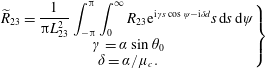
Figure 5. Geometric relations on the cross-stream plane.
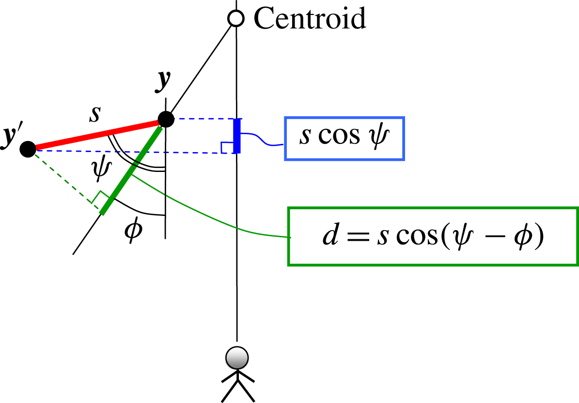
Figure 6. Geometric relations in shifted coordinate system on the cross-stream plane. Without loss of generality, the observer is placed at
 $\unicode[STIX]{x1D719}_{0}=0$
.
$\unicode[STIX]{x1D719}_{0}=0$
.
Equation (3.26) entails integration over the cross-stream plane. Its evaluation is facilitated by examining key geometric relations on this plane. Figure 5 depicts the projections of source elements
 $\boldsymbol{y}$
and
$\boldsymbol{y}$
and
 $\boldsymbol{y}^{\prime }$
and the resulting geometric relations on the cross-stream plane, with the observer located at azimuthal angle
$\boldsymbol{y}^{\prime }$
and the resulting geometric relations on the cross-stream plane, with the observer located at azimuthal angle
 $\unicode[STIX]{x1D719}_{0}$
. All the distances discussed here will be projected distances on the cross-stream plane. The distance between elements
$\unicode[STIX]{x1D719}_{0}$
. All the distances discussed here will be projected distances on the cross-stream plane. The distance between elements
 $\boldsymbol{y}$
and
$\boldsymbol{y}$
and
 $\boldsymbol{y}^{\prime }$
is
$\boldsymbol{y}^{\prime }$
is
 $$\begin{eqnarray}s=\sqrt{y^{\prime 2}+y^{2}-2yy^{\prime }\cos (\unicode[STIX]{x1D719}^{\prime }-\unicode[STIX]{x1D719})}\end{eqnarray}$$
and the projection of this distance on the observer radial line is
 $y^{\prime }\cos (\unicode[STIX]{x1D719}^{\prime }-\unicode[STIX]{x1D719}_{0})-y\cos (\unicode[STIX]{x1D719}-\unicode[STIX]{x1D719}_{0})$
. This is precisely the term that appears in the exponent of (3.26). It thus becomes evident that a coordinate system centred at the source location
$y^{\prime }\cos (\unicode[STIX]{x1D719}^{\prime }-\unicode[STIX]{x1D719}_{0})-y\cos (\unicode[STIX]{x1D719}-\unicode[STIX]{x1D719}_{0})$
. This is precisely the term that appears in the exponent of (3.26). It thus becomes evident that a coordinate system centred at the source location
 $\boldsymbol{y}$
, rather than at the centroid, is preferred for evaluating (3.26). Accordingly, the origin is shifted from the centroid to the location of source element
$\boldsymbol{y}$
, rather than at the centroid, is preferred for evaluating (3.26). Accordingly, the origin is shifted from the centroid to the location of source element
 $\boldsymbol{y}$
, as shown in figure 6. All the azimuthal angles are now defined with respect to the observer angle
$\boldsymbol{y}$
, as shown in figure 6. All the azimuthal angles are now defined with respect to the observer angle
 $\unicode[STIX]{x1D719}_{0}$
. The observer being in the far field, the coordinate shift does not change the angular relations. In the new coordinate system, the azimuthal angle of element
$\unicode[STIX]{x1D719}_{0}$
. The observer being in the far field, the coordinate shift does not change the angular relations. In the new coordinate system, the azimuthal angle of element
 $\boldsymbol{y}^{\prime }$
is
$\boldsymbol{y}^{\prime }$
is
 $\unicode[STIX]{x1D713}$
. The term
$\unicode[STIX]{x1D713}$
. The term
 $y^{\prime }\cos (\unicode[STIX]{x1D719}^{\prime }-\unicode[STIX]{x1D719}_{0})-y\cos (\unicode[STIX]{x1D719}-\unicode[STIX]{x1D719}_{0})$
reduces to
$y^{\prime }\cos (\unicode[STIX]{x1D719}^{\prime }-\unicode[STIX]{x1D719}_{0})-y\cos (\unicode[STIX]{x1D719}-\unicode[STIX]{x1D719}_{0})$
reduces to
 $s\cos \unicode[STIX]{x1D713}$
. Changing the integration variables from
$s\cos \unicode[STIX]{x1D713}$
. Changing the integration variables from
 $(y^{\prime },\unicode[STIX]{x1D719}^{\prime })$
to
$(y^{\prime },\unicode[STIX]{x1D719}^{\prime })$
to
 $(s,\unicode[STIX]{x1D713})$
we obtain
$(s,\unicode[STIX]{x1D713})$
we obtain
 $$\begin{eqnarray}\left.\begin{array}{@{}c@{}}\displaystyle \widetilde{R}_{23}=\frac{1}{\unicode[STIX]{x03C0}L_{23}^{2}}\int _{-\unicode[STIX]{x03C0}}^{\unicode[STIX]{x03C0}}\int _{0}^{\infty }R_{23}\text{e}^{\text{i}\unicode[STIX]{x1D6FE}s\cos \unicode[STIX]{x1D713}-\text{i}\unicode[STIX]{x1D6FF}d}s\,\text{d}s\,\text{d}\unicode[STIX]{x1D713}\\ \unicode[STIX]{x1D6FE}=\unicode[STIX]{x1D6FC}\sin \unicode[STIX]{x1D703}_{0}\\ \displaystyle \unicode[STIX]{x1D6FF}=\unicode[STIX]{x1D6FC}/\unicode[STIX]{x1D707}_{c}.\end{array}\right\}\end{eqnarray}$$
Although an exhaustive treatise of this integral is beyond the scope of the current work, a straightforward strategy for satisfying the requirement of real non-negativeness will be set forth by invoking the integral representation of the Bessel function of the first kind and of order zero:
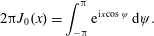 $$\begin{eqnarray}2\unicode[STIX]{x03C0}J_{0}(x)=\int _{-\unicode[STIX]{x03C0}}^{\unicode[STIX]{x03C0}}\text{e}^{\text{i}x\cos \unicode[STIX]{x1D713}}\,\text{d}\unicode[STIX]{x1D713}.\end{eqnarray}$$
First, if
 $d$
is related to
$d$
is related to
 $s$
through a projection of the type
$s$
through a projection of the type
 $d=s\cos (\unicode[STIX]{x1D713}-\unicode[STIX]{x1D712})$
, where
$d=s\cos (\unicode[STIX]{x1D713}-\unicode[STIX]{x1D712})$
, where
 $\unicode[STIX]{x1D712}$
is a reference angle, integration over
$\unicode[STIX]{x1D712}$
is a reference angle, integration over
 $\unicode[STIX]{x1D713}$
yields
$\unicode[STIX]{x1D713}$
yields
 $2\unicode[STIX]{x03C0}J_{0}(\unicode[STIX]{x1D701}s)$
, where
$2\unicode[STIX]{x03C0}J_{0}(\unicode[STIX]{x1D701}s)$
, where
 $\unicode[STIX]{x1D701}$
is a real positive number. Then, on selecting
$\unicode[STIX]{x1D701}$
is a real positive number. Then, on selecting
 $R_{23}=R_{23}(s)$
, the integral over
$R_{23}=R_{23}(s)$
, the integral over
 $s$
becomes the Hankel transform of
$s$
becomes the Hankel transform of
 $R_{23}$
. Here the natural choice for
$R_{23}$
. Here the natural choice for
 $d$
is
$d$
is
 $$\begin{eqnarray}d=s\cos (\unicode[STIX]{x1D713}-\unicode[STIX]{x1D719})=y^{\prime }\cos (\unicode[STIX]{x1D719}^{\prime }-\unicode[STIX]{x1D719})-y,\end{eqnarray}$$
that is,
 $d$
is the projection of
$d$
is the projection of
 $s$
on the radial
$s$
on the radial
 $\unicode[STIX]{x1D719}$
. Integration over
$\unicode[STIX]{x1D719}$
. Integration over
 $\unicode[STIX]{x1D713}$
results in a Bessel function, and (3.28) becomes
$\unicode[STIX]{x1D713}$
results in a Bessel function, and (3.28) becomes
 $$\begin{eqnarray}\widetilde{R}_{23}=\frac{2}{L_{23}^{2}}\int _{0}^{\infty }R_{23}(s)J_{0}\left(s\sqrt{\unicode[STIX]{x1D6FE}^{2}+\unicode[STIX]{x1D6FF}^{2}-2\unicode[STIX]{x1D6FE}\unicode[STIX]{x1D6FF}\cos (\unicode[STIX]{x1D719}-\unicode[STIX]{x1D719}_{0})}\right)s\,\text{d}s\end{eqnarray}$$
yielding the Hankel transform of
 $R_{23}(s)$
. For computational efficiency, we seek forms for
$R_{23}(s)$
. For computational efficiency, we seek forms for
 $R_{23}(s)$
that result in analytical, non-negative solutions (see appendix A for further discussion). Among several candidates, a Gaussian kernel satisfies these conditions and yields a simple analytical solution (Bateman Reference Bateman1954). Accordingly, we select
$R_{23}(s)$
that result in analytical, non-negative solutions (see appendix A for further discussion). Among several candidates, a Gaussian kernel satisfies these conditions and yields a simple analytical solution (Bateman Reference Bateman1954). Accordingly, we select
 $$\begin{eqnarray}R_{23}(s)=\exp \left[-\left(\frac{s}{L_{23}}\right)^{\unicode[STIX]{x1D6FD}_{23}}\right]\end{eqnarray}$$
and restrict
 $\unicode[STIX]{x1D6FD}_{23}=2$
. Evaluation of the Hankel transform gives
$\unicode[STIX]{x1D6FD}_{23}=2$
. Evaluation of the Hankel transform gives
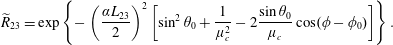 $$\begin{eqnarray}\widetilde{R}_{23}=\exp \left\{-\left(\frac{\unicode[STIX]{x1D6FC}L_{23}}{2}\right)^{2}\left[\sin ^{2}\unicode[STIX]{x1D703}_{0}+\frac{1}{\unicode[STIX]{x1D707}_{c}^{2}}-2\frac{\sin \unicode[STIX]{x1D703}_{0}}{\unicode[STIX]{x1D707}_{c}}\cos (\unicode[STIX]{x1D719}-\unicode[STIX]{x1D719}_{0})\right]\right\}.\end{eqnarray}$$
Therefore, we satisfy the requirement for a real non-negative spectral density. Note that
 $R_{23}$
is periodic with the azimuthal separation
$R_{23}$
is periodic with the azimuthal separation
 $\unicode[STIX]{x1D719}^{\prime }-\unicode[STIX]{x1D719}$
, as is readily observed by inserting (3.27) in (3.32). Importantly, the term
$\unicode[STIX]{x1D719}^{\prime }-\unicode[STIX]{x1D719}$
, as is readily observed by inserting (3.27) in (3.32). Importantly, the term
 $\cos (\unicode[STIX]{x1D719}-\unicode[STIX]{x1D719}_{0})$
in (3.33) induces an azimuthal influence that simulates the effect of suppressed communication through the jet flow discussed in § 2.2.
$\cos (\unicode[STIX]{x1D719}-\unicode[STIX]{x1D719}_{0})$
in (3.33) induces an azimuthal influence that simulates the effect of suppressed communication through the jet flow discussed in § 2.2.
3.5.4 Azimuthal influence
The azimuthal directivity of
 $\widetilde{R}_{23}$
arises from the term
$\widetilde{R}_{23}$
arises from the term
 $\cos (\unicode[STIX]{x1D719}-\unicode[STIX]{x1D719}_{0})$
in (3.33) and is directly controlled by the transverse convective Mach number
$\cos (\unicode[STIX]{x1D719}-\unicode[STIX]{x1D719}_{0})$
in (3.33) and is directly controlled by the transverse convective Mach number
 $\unicode[STIX]{x1D707}_{c}$
. For
$\unicode[STIX]{x1D707}_{c}$
. For
 $\unicode[STIX]{x1D707}_{c}=\infty$
,
$\unicode[STIX]{x1D707}_{c}=\infty$
,
 $\widetilde{R}_{23}$
does not have an azimuthal variation. For
$\widetilde{R}_{23}$
does not have an azimuthal variation. For
 $\unicode[STIX]{x1D707}_{c}$
finite and positive, the azimuthal influence has an extent that is controlled by
$\unicode[STIX]{x1D707}_{c}$
finite and positive, the azimuthal influence has an extent that is controlled by
 $\unicode[STIX]{x1D707}_{c}$
and by the transverse non-dimensional wavenumber
$\unicode[STIX]{x1D707}_{c}$
and by the transverse non-dimensional wavenumber
 $\unicode[STIX]{x1D6FC}L_{23}$
. Figure 7 illustrates these dependencies for observer polar angle
$\unicode[STIX]{x1D6FC}L_{23}$
. Figure 7 illustrates these dependencies for observer polar angle
 $\unicode[STIX]{x1D703}_{0}=30^{\circ }$
. At fixed
$\unicode[STIX]{x1D703}_{0}=30^{\circ }$
. At fixed
 $\unicode[STIX]{x1D6FC}L_{23}$
, the strongest azimuthal directivity is obtained for
$\unicode[STIX]{x1D6FC}L_{23}$
, the strongest azimuthal directivity is obtained for
 $\unicode[STIX]{x1D707}_{c}=1/\sin \unicode[STIX]{x1D703}_{0}$
(
$\unicode[STIX]{x1D707}_{c}=1/\sin \unicode[STIX]{x1D703}_{0}$
(
 $\unicode[STIX]{x1D707}_{c}=2$
in this example). At fixed
$\unicode[STIX]{x1D707}_{c}=2$
in this example). At fixed
 $\unicode[STIX]{x1D707}_{c}$
, the directivity sharpens with increasing
$\unicode[STIX]{x1D707}_{c}$
, the directivity sharpens with increasing
 $\unicode[STIX]{x1D6FC}L_{23}$
(increasing frequency). These observations would tempt one to set
$\unicode[STIX]{x1D6FC}L_{23}$
(increasing frequency). These observations would tempt one to set
 $\unicode[STIX]{x1D707}_{c}=1/\sin \unicode[STIX]{x1D703}_{0}$
to maximize the azimuthal influence. Of course, this is not a legitimate step because the correlation parameters should be independent of observer location. The approach in this study is to set
$\unicode[STIX]{x1D707}_{c}=1/\sin \unicode[STIX]{x1D703}_{0}$
to maximize the azimuthal influence. Of course, this is not a legitimate step because the correlation parameters should be independent of observer location. The approach in this study is to set
 $$\begin{eqnarray}\unicode[STIX]{x1D707}_{c}=\frac{1}{\sin \unicode[STIX]{x1D703}_{peak}},\end{eqnarray}$$
where
 $\unicode[STIX]{x1D703}_{peak}$
is the angle of peak emission, in terms of the overall sound pressure level, for the baseline axisymmetric jet. The combined influence of
$\unicode[STIX]{x1D703}_{peak}$
is the angle of peak emission, in terms of the overall sound pressure level, for the baseline axisymmetric jet. The combined influence of
 $\unicode[STIX]{x1D707}_{c}$
and
$\unicode[STIX]{x1D707}_{c}$
and
 $L_{23}$
on the azimuthal influence places some constraints on the transverse correlation scale
$L_{23}$
on the azimuthal influence places some constraints on the transverse correlation scale
 $L_{23}$
. Specifically, a lower constraint should be placed on the coefficient that controls
$L_{23}$
. Specifically, a lower constraint should be placed on the coefficient that controls
 $L_{23}$
such that, at given frequency,
$L_{23}$
such that, at given frequency,
 $\unicode[STIX]{x1D6FC}L_{23}$
is not too small. The present model for
$\unicode[STIX]{x1D6FC}L_{23}$
is not too small. The present model for
 $\unicode[STIX]{x1D707}_{c}$
is selected for its simplicity. More sophisticated models, where
$\unicode[STIX]{x1D707}_{c}$
is selected for its simplicity. More sophisticated models, where
 $\unicode[STIX]{x1D707}_{c}$
depends on flow conditions and frequency, may provide higher levels of fidelity.
$\unicode[STIX]{x1D707}_{c}$
depends on flow conditions and frequency, may provide higher levels of fidelity.
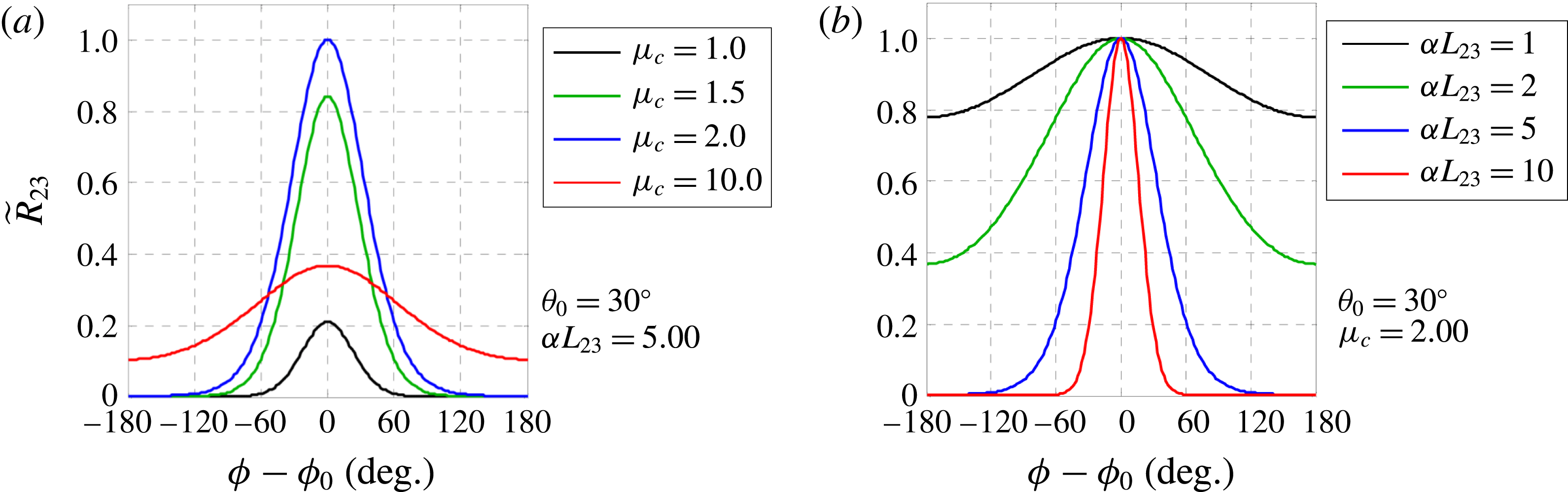
Figure 7. Azimuthal distribution of
 $\widetilde{R}_{23}$
for observer polar angle
$\widetilde{R}_{23}$
for observer polar angle
 $\unicode[STIX]{x1D703}_{0}=30^{\circ }$
. (a) Fixed
$\unicode[STIX]{x1D703}_{0}=30^{\circ }$
. (a) Fixed
 $\unicode[STIX]{x1D6FC}L_{23}$
and varying
$\unicode[STIX]{x1D6FC}L_{23}$
and varying
 $\unicode[STIX]{x1D707}_{c}$
; (b) fixed
$\unicode[STIX]{x1D707}_{c}$
; (b) fixed
 $\unicode[STIX]{x1D707}_{c}$
and varying
$\unicode[STIX]{x1D707}_{c}$
and varying
 $\unicode[STIX]{x1D6FC}L_{23}$
.
$\unicode[STIX]{x1D6FC}L_{23}$
.
3.6 Amplitude of the correlation
The amplitude
 $A_{ijkl}$
in (3.19) represents the correlation
$A_{ijkl}$
in (3.19) represents the correlation
 $$\begin{eqnarray}R_{ijkl}(\boldsymbol{y},\boldsymbol{y},0)=\overline{\unicode[STIX]{x1D61B}_{ij}(\boldsymbol{y},t)\unicode[STIX]{x1D61B}_{kl}(\boldsymbol{y},t)}.\end{eqnarray}$$
It is important to recall, however, that the source term in (3.8) is not
 $R_{ijkl}$
itself but
$R_{ijkl}$
itself but
 $\unicode[STIX]{x2202}^{4}R_{ijkl}/\unicode[STIX]{x2202}\unicode[STIX]{x1D70F}^{4}$
. This means that only terms that depend on
$\unicode[STIX]{x2202}^{4}R_{ijkl}/\unicode[STIX]{x2202}\unicode[STIX]{x1D70F}^{4}$
. This means that only terms that depend on
 $\unicode[STIX]{x1D70F}$
can contribute to
$\unicode[STIX]{x1D70F}$
can contribute to
 $A_{ijkl}$
. It is thus convenient to express
$A_{ijkl}$
. It is thus convenient to express
 $A_{ijkl}$
as
$A_{ijkl}$
as
 $$\begin{eqnarray}A_{ijkl}(\boldsymbol{y})=\overline{[\unicode[STIX]{x1D61B}_{ij}]_{a}[\unicode[STIX]{x1D61B}_{kl}]_{b}},\quad a\rightarrow b,\end{eqnarray}$$
where
 $a$
and
$a$
and
 $b$
represent different times. Only correlations that involve both
$b$
represent different times. Only correlations that involve both
 $a$
and
$a$
and
 $b$
are to be retained.
$b$
are to be retained.
We assume that the principal component of the Lighthill stress tensor is
 $\unicode[STIX]{x1D61B}_{ij}=\overline{\unicode[STIX]{x1D70C}}u_{i}u_{j}$
and write the velocity components as
$\unicode[STIX]{x1D61B}_{ij}=\overline{\unicode[STIX]{x1D70C}}u_{i}u_{j}$
and write the velocity components as
 $$\begin{eqnarray}\left.\begin{array}{@{}c@{}}\displaystyle u_{1}=\overline{u}+u^{\prime }\\ \displaystyle u_{2}=v^{\prime }\\ u_{3}=w^{\prime },\end{array}\right\}\end{eqnarray}$$
where
 $u^{\prime },v^{\prime },w^{\prime }$
are the fluctuating velocity components in Cartesian coordinates. The distinct Lighthill tensor components are
$u^{\prime },v^{\prime },w^{\prime }$
are the fluctuating velocity components in Cartesian coordinates. The distinct Lighthill tensor components are
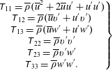 $$\begin{eqnarray}\left.\begin{array}{@{}c@{}}\displaystyle \unicode[STIX]{x1D61B}_{11}=\overline{\unicode[STIX]{x1D70C}}(\overline{u}^{2}+2\overline{u}u^{\prime }+u^{\prime }u^{\prime })\\ \displaystyle \unicode[STIX]{x1D61B}_{12}=\overline{\unicode[STIX]{x1D70C}}(\overline{u}v^{\prime }+u^{\prime }v^{\prime })\\ \displaystyle \unicode[STIX]{x1D61B}_{13}=\overline{\unicode[STIX]{x1D70C}}(\overline{u}w^{\prime }+u^{\prime }w^{\prime })\\ \displaystyle \unicode[STIX]{x1D61B}_{22}=\overline{\unicode[STIX]{x1D70C}}v^{\prime }v^{\prime }\\ \displaystyle \unicode[STIX]{x1D61B}_{23}=\overline{\unicode[STIX]{x1D70C}}v^{\prime }w^{\prime }\\ \displaystyle \unicode[STIX]{x1D61B}_{33}=\overline{\unicode[STIX]{x1D70C}}w^{\prime }w^{\prime }.\end{array}\right\}\end{eqnarray}$$
Following the rule accompanying (3.36), only cross-terms like
 $\overline{u_{a}^{\prime }v_{b}^{\prime }}$
will be retained; terms like
$\overline{u_{a}^{\prime }v_{b}^{\prime }}$
will be retained; terms like
 $\overline{u_{a}^{\prime }v_{a}^{\prime }}$
do not contribute to the source. Under the assumption of isotropic turbulence, the volume integral of the third-order correlations vanishes (Ribner Reference Ribner1969). Although the validity of this assumption needs to be evaluated thoroughly, here we will neglect third-order correlations like
$\overline{u_{a}^{\prime }v_{a}^{\prime }}$
do not contribute to the source. Under the assumption of isotropic turbulence, the volume integral of the third-order correlations vanishes (Ribner Reference Ribner1969). Although the validity of this assumption needs to be evaluated thoroughly, here we will neglect third-order correlations like
 $\overline{u_{a}^{\prime }v_{b}^{\prime 2}}$
. The resulting evaluation of
$\overline{u_{a}^{\prime }v_{b}^{\prime 2}}$
. The resulting evaluation of
 $A_{ijkl}$
leads to terms containing second-order correlations
$A_{ijkl}$
leads to terms containing second-order correlations
 $\overline{u_{i}^{\prime }u_{j}^{\prime }}$
, usually referred to as ‘shear noise’; and terms containing fourth-order correlations
$\overline{u_{i}^{\prime }u_{j}^{\prime }}$
, usually referred to as ‘shear noise’; and terms containing fourth-order correlations
 $\overline{u_{i}^{\prime }u_{j}^{\prime }u_{k}^{\prime }u_{l}^{\prime }}$
, typically described as ‘self-noise’. A preliminary evaluation of the self-noise terms, using the quasi-normal hypothesis (Morris & Zaman Reference Morris and Zaman2010b
) and the approximations that follow, indicates that their contribution to peak noise is at least 10 dB below the contribution of the shear-noise terms. Therefore, the fourth-order correlations are deemed irrelevant to the prediction of peak noise.
$\overline{u_{i}^{\prime }u_{j}^{\prime }u_{k}^{\prime }u_{l}^{\prime }}$
, typically described as ‘self-noise’. A preliminary evaluation of the self-noise terms, using the quasi-normal hypothesis (Morris & Zaman Reference Morris and Zaman2010b
) and the approximations that follow, indicates that their contribution to peak noise is at least 10 dB below the contribution of the shear-noise terms. Therefore, the fourth-order correlations are deemed irrelevant to the prediction of peak noise.
Figure 8. Azimuthal relationships of source and observer.
Thus, the problem boils down to modelling the second-order correlations, that is, the components of the Reynolds stress tensor. To this end, we use the constitutive relation that forms the foundation of turbulence modelling (Mathieu & Scott Reference Mathieu and Scott2000)
 $$\begin{eqnarray}\overline{u_{i}^{\prime }u_{j}^{\prime }}={\textstyle \frac{2}{3}}k\unicode[STIX]{x1D6FF}_{ij}-\unicode[STIX]{x1D708}_{T}S_{ij},\end{eqnarray}$$
where
 $\unicode[STIX]{x1D708}_{T}$
is the turbulent viscosity,
$\unicode[STIX]{x1D708}_{T}$
is the turbulent viscosity,
 $\unicode[STIX]{x1D6FF}_{ij}$
is the Kronecker delta and
$\unicode[STIX]{x1D6FF}_{ij}$
is the Kronecker delta and
 $$\begin{eqnarray}S_{ij}=\frac{\unicode[STIX]{x2202}\overline{u}_{i}}{\unicode[STIX]{x2202}x_{j}}+\frac{\unicode[STIX]{x2202}\overline{u}_{j}}{\unicode[STIX]{x2202}x_{i}}.\end{eqnarray}$$
Given that the jet flow is slowly diverging, the dominant component of
 $S_{ij}$
is the transverse gradient of the mean axial velocity. The approximate magnitude of this gradient is
$S_{ij}$
is the transverse gradient of the mean axial velocity. The approximate magnitude of this gradient is
 $$\begin{eqnarray}G=\sqrt{\left[\frac{\unicode[STIX]{x2202}\overline{u}}{\unicode[STIX]{x2202}Y}\right]^{2}+\left[\frac{\unicode[STIX]{x2202}\overline{u}}{\unicode[STIX]{x2202}Z}\right]^{2}}\end{eqnarray}$$
and its azimuthal direction is
 $\unicode[STIX]{x1D719}_{g}$
. Figure 8 describes the azimuthal relations between source and observer. The convention here is to assign an outward azimuthal direction for an inward gradient, and vice versa. For an axisymmetric jet with monotonically declining radial velocity profile (that is, without a wake component),
$\unicode[STIX]{x1D719}_{g}$
. Figure 8 describes the azimuthal relations between source and observer. The convention here is to assign an outward azimuthal direction for an inward gradient, and vice versa. For an axisymmetric jet with monotonically declining radial velocity profile (that is, without a wake component),
 $\unicode[STIX]{x1D719}_{g}$
coincides with the geometric azimuthal angle
$\unicode[STIX]{x1D719}_{g}$
coincides with the geometric azimuthal angle
 $\unicode[STIX]{x1D719}$
. For a jet whose velocity isocontours are not circular, or that has a wake defect,
$\unicode[STIX]{x1D719}$
. For a jet whose velocity isocontours are not circular, or that has a wake defect,
 $\unicode[STIX]{x1D719}_{g}$
and
$\unicode[STIX]{x1D719}_{g}$
and
 $\unicode[STIX]{x1D719}$
will generally be different.
$\unicode[STIX]{x1D719}$
will generally be different.
It is now argued that the principal turbulent transport is in the direction of the mean flow gradient with an associated turbulent velocity fluctuation
 $q^{\prime }$
. The corresponding velocity correlation
$q^{\prime }$
. The corresponding velocity correlation
 $$\begin{eqnarray}g=\langle u^{\prime }q^{\prime }\rangle =\unicode[STIX]{x1D708}_{T}G\end{eqnarray}$$
is deemed the dominant contributor to the momentum transport and hence to the Reynolds stress. The transport normal to the direction of the mean flow gradient is considered negligible. The correlation
 $g$
will henceforth be loosely referred to as the ‘Reynolds stress’ and will be treated as non-negative. The direction of the mean flow gradient, and its impact on the individual terms of the Reynolds stress tensor, will be accounted for by the angle
$g$
will henceforth be loosely referred to as the ‘Reynolds stress’ and will be treated as non-negative. The direction of the mean flow gradient, and its impact on the individual terms of the Reynolds stress tensor, will be accounted for by the angle
 $\unicode[STIX]{x1D719}_{g}$
. Returning to the constitutive relation (3.39), using
$\unicode[STIX]{x1D719}_{g}$
. Returning to the constitutive relation (3.39), using
 $v^{\prime }=-q^{\prime }\cos \unicode[STIX]{x1D719}_{g}$
and
$v^{\prime }=-q^{\prime }\cos \unicode[STIX]{x1D719}_{g}$
and
 $w^{\prime }=q^{\prime }\sin \unicode[STIX]{x1D719}_{g}$
, we are now able to make the following approximations:
$w^{\prime }=q^{\prime }\sin \unicode[STIX]{x1D719}_{g}$
, we are now able to make the following approximations:
 $$\begin{eqnarray}\left.\begin{array}{@{}c@{}}\displaystyle \overline{u^{\prime }u^{\prime }}\approx {\textstyle \frac{2}{3}}k\\ \displaystyle \overline{v^{\prime }v^{\prime }}\approx {\textstyle \frac{2}{3}}k\\ \displaystyle \overline{w^{\prime }w^{\prime }}\approx {\textstyle \frac{2}{3}}k\\ \overline{u^{\prime }v^{\prime }}=-\langle u^{\prime }q^{\prime }\rangle \displaystyle \cos \unicode[STIX]{x1D719}_{g}\approx -g\cos \unicode[STIX]{x1D719}_{g}\\ \overline{u^{\prime }w^{\prime }}=\langle u^{\prime }q^{\prime }\rangle \displaystyle \sin \unicode[STIX]{x1D719}_{g}\approx g\sin \unicode[STIX]{x1D719}_{g}\\ \overline{v^{\prime }w^{\prime }}\approx 0.\end{array}\right\}\end{eqnarray}$$
It is recognized that in the actual jet the axial velocity fluctuations are stronger than the transverse fluctuations, as measured by a variety of experiments (for example, Morris & Zaman Reference Morris and Zaman2010b ). However, here it is preferred to stay faithful to the constitutive relation (3.39).
Based on the convention of figure 2, the direction cosines for the far-field observer are
 $$\begin{eqnarray}\left.\begin{array}{@{}c@{}}\displaystyle \unicode[STIX]{x1D717}_{1}=\cos \unicode[STIX]{x1D703}_{0}\\ \displaystyle \unicode[STIX]{x1D717}_{2}=-\!\sin \unicode[STIX]{x1D703}_{0}\cos \unicode[STIX]{x1D719}_{0}\\ \displaystyle \unicode[STIX]{x1D717}_{3}=\sin \unicode[STIX]{x1D703}_{0}\sin \unicode[STIX]{x1D719}_{0}.\end{array}\right\}\end{eqnarray}$$
Due to the symmetry of
 $\unicode[STIX]{x1D61B}_{ij}$
and the resulting pairwise symmetry of
$\unicode[STIX]{x1D61B}_{ij}$
and the resulting pairwise symmetry of
 $A_{ijkl}$
(that is,
$A_{ijkl}$
(that is,
 $A_{ijkl}=A_{klij}$
), the 81 elements of
$A_{ijkl}=A_{klij}$
), the 81 elements of
 $A_{ijkl}$
comprise single or multiple occurrences of 21 distinct terms. Of those, only 6 terms have the potential to contribute to shear noise; these are the terms where the index
$A_{ijkl}$
comprise single or multiple occurrences of 21 distinct terms. Of those, only 6 terms have the potential to contribute to shear noise; these are the terms where the index
 $1$
appears at least once in
$1$
appears at least once in
 $ij$
and at least once in
$ij$
and at least once in
 $kl$
. Table 1 lists the shear-noise terms, their multipliers (frequencies), their expressions according to (3.38), their approximations according to (3.43) and their directivities according to (3.44).
$kl$
. Table 1 lists the shear-noise terms, their multipliers (frequencies), their expressions according to (3.38), their approximations according to (3.43) and their directivities according to (3.44).
Table 1. Distinct shear-noise terms of
 $A_{ijkl}$
and associated directivities.
$A_{ijkl}$
and associated directivities.
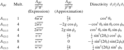
The total contribution in the direction of the far-field observer is
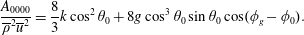 $$\begin{eqnarray}\frac{A_{0000}}{\overline{\unicode[STIX]{x1D70C}}^{2}\overline{u}^{2}}=\frac{8}{3}k\cos ^{2}\unicode[STIX]{x1D703}_{0}+8g\cos ^{3}\unicode[STIX]{x1D703}_{0}\sin \unicode[STIX]{x1D703}_{0}\cos (\unicode[STIX]{x1D719}_{g}-\unicode[STIX]{x1D719}_{0}).\end{eqnarray}$$
The second term on the right-hand side arises from the 1112 and 1113 components of the Lighthill stress tensor. In past works on axisymmetric jets, these components were neglected because they were thought to integrate to zero when inserted in the formula for the spectral density (Ribner Reference Ribner1969). This is not the case if we accept that the space–time correlation induces an azimuthal directivity along the lines of (3.33). Then, the second term of (3.45) does not integrate to zero and makes a finite, positive contribution to the spectral density. Of course, the components
 $A_{1112}$
and
$A_{1112}$
and
 $A_{1113}$
must be retained for asymmetric jets regardless of the chosen form of the space–time correlation.
$A_{1113}$
must be retained for asymmetric jets regardless of the chosen form of the space–time correlation.
The azimuthal dependencies contained in the cosine terms of (3.33) and (3.45) complicate the evaluation of the spectral density (3.25) when the computational domain is restricted to one of the symmetric halves of the jet flow. In addition, for axisymmetric jets, it is desirable to cut down the expense of computing the spectral density by considering only an azimuthal slice of the domain, a task also complicated by the cosine terms. These issues are addressed in appendix A.
3.7 Outer surface of peak stress (OSPS)
In the expression for the spectral density (3.25), the effect of the axial convection of the turbulent eddies is captured by the term
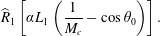 $$\begin{eqnarray}\widehat{R}_{1}\left[\unicode[STIX]{x1D6FC}L_{1}\left(\frac{1}{M_{c}}-\cos \unicode[STIX]{x1D703}_{0}\right)\right].\end{eqnarray}$$
We will call this term ‘radiation efficiency’, realizing that this term has been used in the past under varying contexts. Here it means the efficiency with which a four-dimensional correlation volume
 $\unicode[STIX]{x1D70F}_{\ast }L_{1}\unicode[STIX]{x03C0}L_{23}^{2}$
radiates sound to the far field at fixed amplitude, frequency and correlation functions. The radiation efficiency is controlled by the convective Mach number
$\unicode[STIX]{x1D70F}_{\ast }L_{1}\unicode[STIX]{x03C0}L_{23}^{2}$
radiates sound to the far field at fixed amplitude, frequency and correlation functions. The radiation efficiency is controlled by the convective Mach number
 $M_{c}=U_{c}/a_{\infty }$
. We gain insight into the underlying physics by considering special values of
$M_{c}=U_{c}/a_{\infty }$
. We gain insight into the underlying physics by considering special values of
 $M_{c}$
. For a very low-speed jet where
$M_{c}$
. For a very low-speed jet where
 $M_{c}\rightarrow 0$
, the argument of
$M_{c}\rightarrow 0$
, the argument of
 $\widehat{R}_{1}$
becomes very large and thus
$\widehat{R}_{1}$
becomes very large and thus
 $\widehat{R}_{1}\rightarrow 0$
. This is the limit of zero radiation efficiency. The limit
$\widehat{R}_{1}\rightarrow 0$
. This is the limit of zero radiation efficiency. The limit
 $M_{c}=\infty$
signifies disturbances being transmitted instantaneously throughout the length of the object, like in the case of an oscillating solid cylinder. Then the radiation efficiency becomes
$M_{c}=\infty$
signifies disturbances being transmitted instantaneously throughout the length of the object, like in the case of an oscillating solid cylinder. Then the radiation efficiency becomes
 $\widehat{R}_{1}(-\unicode[STIX]{x1D6FC}L_{1}\cos \unicode[STIX]{x1D703}_{0})$
and the peak radiation occurs at
$\widehat{R}_{1}(-\unicode[STIX]{x1D6FC}L_{1}\cos \unicode[STIX]{x1D703}_{0})$
and the peak radiation occurs at
 $\unicode[STIX]{x1D703}_{0}=90^{\circ }$
. In general, the radiation efficiency peaks at
$\unicode[STIX]{x1D703}_{0}=90^{\circ }$
. In general, the radiation efficiency peaks at
 $\cos \unicode[STIX]{x1D703}_{0}=1/M_{c}$
, where the argument of
$\cos \unicode[STIX]{x1D703}_{0}=1/M_{c}$
, where the argument of
 $R_{1}$
is zero. For
$R_{1}$
is zero. For
 $M_{c}\geqslant 1$
, this represents the well-known Mach wave emission in high-speed jets that occurs near
$M_{c}\geqslant 1$
, this represents the well-known Mach wave emission in high-speed jets that occurs near
 $\unicode[STIX]{x1D703}_{0}=\arccos (1/M_{c})$
. For
$\unicode[STIX]{x1D703}_{0}=\arccos (1/M_{c})$
. For
 $M_{c}<1$
the radiation efficiency does not reach its peak value and increases monotonically towards
$M_{c}<1$
the radiation efficiency does not reach its peak value and increases monotonically towards
 $\unicode[STIX]{x1D703}_{0}=0$
. A physical constraint in applying the above arguments is the spreading rate of the jet flow, which is around 10
$\unicode[STIX]{x1D703}_{0}=0$
. A physical constraint in applying the above arguments is the spreading rate of the jet flow, which is around 10
 $^{\circ }$
. Sound emission at observer angles close to the spreading angle is bound to be influenced by flow–acoustic interactions.
$^{\circ }$
. Sound emission at observer angles close to the spreading angle is bound to be influenced by flow–acoustic interactions.
The importance of the radiation efficiency term, coupled with the need to connect it to sound generated by coherent structures, make the selection of
 $M_{c}$
one of the most critical decisions in the modelling. Here we argue that radiation efficiency is governed by the eddies of the outermost shear layer of the jet. This follows the observation that just outside the jet, in the near pressure field, the pressure distribution reflects the ‘footprint’ of the most energetic eddies, as confirmed by several studies of single-stream jets (Ho Reference Ho1985; Zaman Reference Zaman1986). For multistream jets, we pose an additional condition that these eddies be in direct contact with the ambient fluid, a position supported by recent measurements of the convective velocity in the near field of dual-stream jets (Papamoschou & Phong Reference Papamoschou and Phong2017). The noise radiated by the outer eddies involves a direct coupling between the turbulent motion and the sound field; this does not involve mean flow/acoustic interaction or propagation effects as long as the observer polar angle is not too close to the jet spreading angle. In terms of the mean flow, and following the arguments presented in § 2.1, the action of these eddies is represented by the peak Reynolds stress of the outermost shear layer. Accordingly, we define the outer surface of peak stress (OSPS) as the locus of the first peak of the Reynolds stress as one approaches the jet from the ambient towards the jet axis. Denoting the radial location of the OSPS as
$M_{c}$
one of the most critical decisions in the modelling. Here we argue that radiation efficiency is governed by the eddies of the outermost shear layer of the jet. This follows the observation that just outside the jet, in the near pressure field, the pressure distribution reflects the ‘footprint’ of the most energetic eddies, as confirmed by several studies of single-stream jets (Ho Reference Ho1985; Zaman Reference Zaman1986). For multistream jets, we pose an additional condition that these eddies be in direct contact with the ambient fluid, a position supported by recent measurements of the convective velocity in the near field of dual-stream jets (Papamoschou & Phong Reference Papamoschou and Phong2017). The noise radiated by the outer eddies involves a direct coupling between the turbulent motion and the sound field; this does not involve mean flow/acoustic interaction or propagation effects as long as the observer polar angle is not too close to the jet spreading angle. In terms of the mean flow, and following the arguments presented in § 2.1, the action of these eddies is represented by the peak Reynolds stress of the outermost shear layer. Accordingly, we define the outer surface of peak stress (OSPS) as the locus of the first peak of the Reynolds stress as one approaches the jet from the ambient towards the jet axis. Denoting the radial location of the OSPS as
 $y_{OSPS}(X,\unicode[STIX]{x1D719})$
, and letting
$y_{OSPS}(X,\unicode[STIX]{x1D719})$
, and letting
 $\boldsymbol{y}=(X,y,\unicode[STIX]{x1D719})$
represent the location of a volume element in polar coordinates (figure 2), the convective Mach number of that element is defined as
$\boldsymbol{y}=(X,y,\unicode[STIX]{x1D719})$
represent the location of a volume element in polar coordinates (figure 2), the convective Mach number of that element is defined as
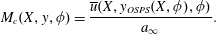 $$\begin{eqnarray}M_{c}(X,y,\unicode[STIX]{x1D719})=\frac{\overline{u}(X,y_{OSPS}(X,\unicode[STIX]{x1D719}),\unicode[STIX]{x1D719})}{a_{\infty }}.\end{eqnarray}$$
This means that all the volume elements at a particular
 $X$
and
$X$
and
 $\unicode[STIX]{x1D719}$
are assigned the same value of
$\unicode[STIX]{x1D719}$
are assigned the same value of
 $M_{c}$
as determined by (3.47).
$M_{c}$
as determined by (3.47).
Accurate detection of the OSPS requires very good resolution of the thin layers near the nozzle exit. The near-field region affects the mid to high frequencies and is thus of paramount importance to aircraft noise. The detection scheme is illustrated in figure 9. The RANS flow field is divided into axial slices of very fine spacing near the nozzle exit and coarser spacing downstream. Each axial slice is divided into fine azimuthal segments, typically in
 $2.5^{\circ }$
increments. Within each azimuthal segment, the data (velocity, Reynolds stress) are sorted in order of the decreasing radius
$2.5^{\circ }$
increments. Within each azimuthal segment, the data (velocity, Reynolds stress) are sorted in order of the decreasing radius
 $y$
. The search process for the first (outermost) peak of the Reynolds stress starts at the radial location where the mean axial velocity is one third of the tertiary exit velocity, a position that is well outside the dividing streamline of the outermost shear layer but still within the jet flow. Starting the search within the jet flow prevents spurious detection of peaks that may occur if one started the search further out where the velocity is very low and the data can be noisy. Denoting
$y$
. The search process for the first (outermost) peak of the Reynolds stress starts at the radial location where the mean axial velocity is one third of the tertiary exit velocity, a position that is well outside the dividing streamline of the outermost shear layer but still within the jet flow. Starting the search within the jet flow prevents spurious detection of peaks that may occur if one started the search further out where the velocity is very low and the data can be noisy. Denoting
 $g_{j}$
the discrete values of the Reynolds stress, the operation
$g_{j}$
the discrete values of the Reynolds stress, the operation
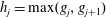 $h_{j}=\max (g_{j},g_{j+1})$
is carried out as we move inward towards the jet axis. We seek the first occurrence where
$h_{j}=\max (g_{j},g_{j+1})$
is carried out as we move inward towards the jet axis. We seek the first occurrence where
 $h_{j}$
remains invariant for
$h_{j}$
remains invariant for
 $J$
consecutive points. This indicates that the first peak of the Reynolds stress occurred at point
$J$
consecutive points. This indicates that the first peak of the Reynolds stress occurred at point
 $j-J$
. The proper value of
$j-J$
. The proper value of
 $J$
will depend on the resolution of the RANS data (population of each axial/azimuthal segment) and needs to be determined carefully by the user. Examples of the OSPS will be shown figures 16–18.
$J$
will depend on the resolution of the RANS data (population of each axial/azimuthal segment) and needs to be determined carefully by the user. Examples of the OSPS will be shown figures 16–18.

Figure 9. Detection scheme for the location of the outer peak of the Reynolds stress (triangular marker).
3.8 RANS-based scales
The correlation length and time scales follow the traditional definitions, based on the RANS flow field, used in past acoustic analogy models (Morris & Farassat Reference Morris and Farassat2002). They are constructed from the turbulent kinetic energy
 $k$
and the dissipation
$k$
and the dissipation
 $\unicode[STIX]{x1D716}$
. The specific dissipation is defined as
$\unicode[STIX]{x1D716}$
. The specific dissipation is defined as
 $\unicode[STIX]{x1D6FA}=\unicode[STIX]{x1D716}/k$
. The equation that follows describes the axial and transverse length scales, and the time scale.
$\unicode[STIX]{x1D6FA}=\unicode[STIX]{x1D716}/k$
. The equation that follows describes the axial and transverse length scales, and the time scale.
 $$\begin{eqnarray}\left.\begin{array}{@{}c@{}}\displaystyle L_{1}=C_{1}\frac{k^{3/2}}{\unicode[STIX]{x1D716}}=C_{1}\frac{k^{1/2}}{\unicode[STIX]{x1D6FA}}\\ \displaystyle L_{23}=C_{23}\frac{k^{3/2}}{\unicode[STIX]{x1D716}}=C_{23}\frac{k^{1/2}}{\unicode[STIX]{x1D6FA}}\\ \displaystyle \unicode[STIX]{x1D70F}_{\ast }=C_{4}\frac{k}{\unicode[STIX]{x1D716}}=C_{4}\frac{1}{\unicode[STIX]{x1D6FA}}.\end{array}\right\}\end{eqnarray}$$
The turbulent viscosity
 $\unicode[STIX]{x1D708}_{T}$
in (3.39) is obtained from the usual dimensional construct
$\unicode[STIX]{x1D708}_{T}$
in (3.39) is obtained from the usual dimensional construct
 $$\begin{eqnarray}\unicode[STIX]{x1D708}_{T}=c_{\unicode[STIX]{x1D707}}\frac{k}{\unicode[STIX]{x1D6FA}}.\end{eqnarray}$$
The value
 $c_{\unicode[STIX]{x1D707}}=0.09$
was used here.
$c_{\unicode[STIX]{x1D707}}=0.09$
was used here.
4 Parameterization of the space–time correlation
The preceding sections described the theoretical framework for calculating the far-field spectral density as summarized in (3.25). The specific implementation of (3.25) requires selection of the parameters that control the shapes of the correlation functions
 $R_{1}$
,
$R_{1}$
,
 $R_{23}$
and
$R_{23}$
and
 $R_{4}$
that comprise the space–time correlation of the Lighthill stress tensor given by (3.19). Here we discuss the process by which these parameters are selected.
$R_{4}$
that comprise the space–time correlation of the Lighthill stress tensor given by (3.19). Here we discuss the process by which these parameters are selected.
4.1 Source parameters
The prediction of the far-field spectral density is dependent on a parameter vector
 $\boldsymbol{V}=(V_{1},\ldots ,V_{K})$
that defines the correlation functions used in formulating the space–time correlation in (3.19). Here the parameter vector comprises the scale coefficients
$\boldsymbol{V}=(V_{1},\ldots ,V_{K})$
that defines the correlation functions used in formulating the space–time correlation in (3.19). Here the parameter vector comprises the scale coefficients
 $C_{1},C_{23},C_{4}$
in (3.48) and the exponent powers
$C_{1},C_{23},C_{4}$
in (3.48) and the exponent powers
 $\unicode[STIX]{x1D6FD}_{1},\unicode[STIX]{x1D6FD}_{4}$
in (3.20). Recall that the exponent power for the cross-stream correlation is fixed at
$\unicode[STIX]{x1D6FD}_{1},\unicode[STIX]{x1D6FD}_{4}$
in (3.20). Recall that the exponent power for the cross-stream correlation is fixed at
 $\unicode[STIX]{x1D6FD}_{23}=2$
.
$\unicode[STIX]{x1D6FD}_{23}=2$
.
We denote the parameter vector
 $$\begin{eqnarray}\boldsymbol{V}=[C_{1},C_{23},C_{4},\unicode[STIX]{x1D6FD}_{1},\unicode[STIX]{x1D6FD}_{4}].\end{eqnarray}$$
The far-field power spectral density can then be expressed as
 $$\begin{eqnarray}S(\boldsymbol{V},{\mathcal{R}},\unicode[STIX]{x1D703}_{0},\unicode[STIX]{x1D719}_{0},\unicode[STIX]{x1D714}).\end{eqnarray}$$
It is convenient to work with the sound pressure level (SPL) spectrum, in units of decibels. The modelled SPL spectrum is
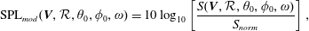 $$\begin{eqnarray}\text{SPL}_{mod}(\boldsymbol{V},{\mathcal{R}},\unicode[STIX]{x1D703}_{0},\unicode[STIX]{x1D719}_{0},\unicode[STIX]{x1D714})=10\log _{10}\left[\frac{S(\boldsymbol{V},{\mathcal{R}},\unicode[STIX]{x1D703}_{0},\unicode[STIX]{x1D719}_{0},\unicode[STIX]{x1D714})}{S_{norm}}\right],\end{eqnarray}$$
where
 $S_{norm}=4\times 10^{-10}~\text{Pa}^{2}$
is the commonly used normalization value. The experimental SPL spectrum is
$S_{norm}=4\times 10^{-10}~\text{Pa}^{2}$
is the commonly used normalization value. The experimental SPL spectrum is
 $\text{SPL}_{exp}({\mathcal{R}}_{exp},\unicode[STIX]{x1D703}_{0},\unicode[STIX]{x1D719}_{0},\unicode[STIX]{x1D714})$
where
$\text{SPL}_{exp}({\mathcal{R}}_{exp},\unicode[STIX]{x1D703}_{0},\unicode[STIX]{x1D719}_{0},\unicode[STIX]{x1D714})$
where
 ${\mathcal{R}}_{exp}$
is the microphone distance or the distance to which the experimental spectrum is referenced.
${\mathcal{R}}_{exp}$
is the microphone distance or the distance to which the experimental spectrum is referenced.
4.2 Determination of parameter vector
Determination of the parameter vector is based on knowledge of the spectral density of the axisymmetric reference jet. Specifically, we seek a parameter vector that minimizes the difference between the modelled and experimental SPL spectra for the reference jet:
 $\text{SPL}_{mod}^{ref}(\boldsymbol{V},R,\unicode[STIX]{x1D703}_{0},\unicode[STIX]{x1D714})$
and
$\text{SPL}_{mod}^{ref}(\boldsymbol{V},R,\unicode[STIX]{x1D703}_{0},\unicode[STIX]{x1D714})$
and
 $\text{SPL}_{exp}^{ref}({\mathcal{R}}_{exp},\unicode[STIX]{x1D703}_{0},\unicode[STIX]{x1D714})$
, respectively. We facilitate the optimization by normalizing the experimental and modelled spectral densities by their respective maximum values versus frequency. Equivalently, in units of decibels we subtract the maximum values. The normalization removes the effect of the distances
$\text{SPL}_{exp}^{ref}({\mathcal{R}}_{exp},\unicode[STIX]{x1D703}_{0},\unicode[STIX]{x1D714})$
, respectively. We facilitate the optimization by normalizing the experimental and modelled spectral densities by their respective maximum values versus frequency. Equivalently, in units of decibels we subtract the maximum values. The normalization removes the effect of the distances
 ${\mathcal{R}}$
and
${\mathcal{R}}$
and
 ${\mathcal{R}}_{exp}$
, so the normalized spectra depend only on the parameter vector (for the modelled spectrum), the observer polar angle and the frequency. The normalized modelled and experimental SPL spectra for the reference jet are:
${\mathcal{R}}_{exp}$
, so the normalized spectra depend only on the parameter vector (for the modelled spectrum), the observer polar angle and the frequency. The normalized modelled and experimental SPL spectra for the reference jet are:
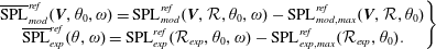 $$\begin{eqnarray}\left.\begin{array}{@{}c@{}}\displaystyle \overline{\text{SPL}}_{mod}^{ref}(\boldsymbol{V},\unicode[STIX]{x1D703}_{0},\unicode[STIX]{x1D714})=\text{SPL}_{mod}^{ref}(\boldsymbol{V},{\mathcal{R}},\unicode[STIX]{x1D703}_{0},\unicode[STIX]{x1D714})-\text{SPL}_{mod,max}^{ref}(\boldsymbol{V},{\mathcal{R}},\unicode[STIX]{x1D703}_{0})\\ \displaystyle \overline{\text{SPL}}_{exp}^{ref}(\unicode[STIX]{x1D703},\unicode[STIX]{x1D714})=\text{SPL}_{exp}^{ref}({\mathcal{R}}_{exp},\unicode[STIX]{x1D703}_{0},\unicode[STIX]{x1D714})-\text{SPL}_{exp,max}^{ref}({\mathcal{R}}_{exp},\unicode[STIX]{x1D703}_{0}).\end{array}\right\}\end{eqnarray}$$
This normalization removes the amplitude as a variable, so we are concerned only with matching the shape of the spectra.
We seek to minimize the difference between the modelled and experimental spectra at observer polar angle
 $\unicode[STIX]{x1D703}_{0}$
and at a set of frequencies
$\unicode[STIX]{x1D703}_{0}$
and at a set of frequencies
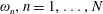 $\unicode[STIX]{x1D714}_{n},n=1,\ldots ,N$
. We construct the cost function
$\unicode[STIX]{x1D714}_{n},n=1,\ldots ,N$
. We construct the cost function
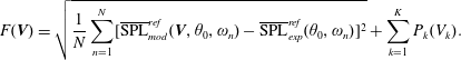 $$\begin{eqnarray}F(\boldsymbol{V})=\sqrt{\frac{1}{N}\mathop{\sum }_{n=1}^{N}[\overline{\text{SPL}}_{mod}^{ref}(\boldsymbol{V},\unicode[STIX]{x1D703}_{0},\unicode[STIX]{x1D714}_{n})-\overline{\text{SPL}}_{exp}^{ref}(\unicode[STIX]{x1D703}_{0},\unicode[STIX]{x1D714}_{n})]^{2}}+\mathop{\sum }_{k=1}^{K}P_{k}(V_{k}).\end{eqnarray}$$
The square root term represents the ‘error’ between model and experiment in units of decibels;
 $P_{k}$
are appropriately defined penalty functions that constrain the parameters within reasonable ranges. The parameter vector
$P_{k}$
are appropriately defined penalty functions that constrain the parameters within reasonable ranges. The parameter vector
 $\boldsymbol{V}$
is determined by minimizing the cost function. The minimization process of (4.5) utilized the restarted conjugate-gradient method of Shanno & Phua (Reference Shanno and Phua1976) (ACM TOM Algorithm 500). The minimization typically used
$\boldsymbol{V}$
is determined by minimizing the cost function. The minimization process of (4.5) utilized the restarted conjugate-gradient method of Shanno & Phua (Reference Shanno and Phua1976) (ACM TOM Algorithm 500). The minimization typically used
 $N=10$
frequencies spaced at equal logarithmic intervals, covering the entire relevant part of the spectrum. The scheme converged after approximately 30 function calls to an error around 1.0 dB and zero penalty function.
$N=10$
frequencies spaced at equal logarithmic intervals, covering the entire relevant part of the spectrum. The scheme converged after approximately 30 function calls to an error around 1.0 dB and zero penalty function.
4.3 Application to non-reference jets
Upon a satisfactory match of the reference modelled and experimental spectra, the parameter vector
 $\boldsymbol{V}$
becomes determined. This parameter vector is now applied to the non-reference (typically asymmetric) jet, yielding
$\boldsymbol{V}$
becomes determined. This parameter vector is now applied to the non-reference (typically asymmetric) jet, yielding
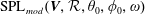 $\text{SPL}_{mod}(\boldsymbol{V},{\mathcal{R}},\unicode[STIX]{x1D703}_{0},\unicode[STIX]{x1D719}_{0},\unicode[STIX]{x1D714})$
. Direct comparison with the SPL spectrum of the experimental non-reference jet is enabled by the amplitude adjustment
$\text{SPL}_{mod}(\boldsymbol{V},{\mathcal{R}},\unicode[STIX]{x1D703}_{0},\unicode[STIX]{x1D719}_{0},\unicode[STIX]{x1D714})$
. Direct comparison with the SPL spectrum of the experimental non-reference jet is enabled by the amplitude adjustment
 $$\begin{eqnarray}\text{SPL}_{mod}(\boldsymbol{V},{\mathcal{R}}_{exp},\unicode[STIX]{x1D703}_{0},\unicode[STIX]{x1D719}_{0},\unicode[STIX]{x1D714})=\text{SPL}_{mod}(\boldsymbol{V},{\mathcal{R}},\unicode[STIX]{x1D703}_{0},\unicode[STIX]{x1D719}_{0},\unicode[STIX]{x1D714})+\text{SPL}_{exp,max}^{ref}-\text{SPL}_{mod,max}^{ref}.\end{eqnarray}$$
5 Application fields
So far we have described a methodology for the acoustic prediction of multistream symmetric and asymmetric jets, and the parameterization of the problem based the far-field sound of the baseline (symmetric) jet. Again, we are interested in predicting the noise change from a known baseline. In this section we describe briefly the experimental and computational data for the jets to which this methodology will be applied. An extensive review of the experimental results is available in Papamoschou et al. (Reference Papamoschou, Phong, Xiong and Liu2016) and Phong & Papamoschou (Reference Phong and Papamoschou2017).
5.1 Experimental
5.1.1 Experimental set-up
The experiments utilized three-stream nozzles as part of UCI’s recent effort in characterizing and suppressing noise from three-stream jets representative of the exhausts of future supersonic aircraft. The nozzles comprised axisymmetric (reference) configurations as well as asymmetric configurations that involved reshaping of the secondary and tertiary ducts that surround the primary duct. The intent of the asymmetric nozzles was to reduce noise directed downward, that is, towards airport communities. This report covers two sets of nozzles, nominal plug and enlarged plug. The enlarged-plug nozzles were motivated by sonic-boom compatibility, as explained in Phong & Papamoschou (Reference Phong and Papamoschou2017). Nozzle naming is consistent with that used in past reports for ease of reference. The subscripts
 $p$
,
$p$
,
 $s$
and
$s$
and
 $t$
are used to denote the primary, secondary and tertiary streams, respectively. Key features of the nozzles are presented in figures 10 and 11 for the nominal- and enlarged-plug sets, respectively, including the azimuthal distributions of the widths of the annuli at the terminations of the secondary and tertiary ducts. All the nozzles share the same exit areas. The effective (area-based) primary exit diameter is
$t$
are used to denote the primary, secondary and tertiary streams, respectively. Key features of the nozzles are presented in figures 10 and 11 for the nominal- and enlarged-plug sets, respectively, including the azimuthal distributions of the widths of the annuli at the terminations of the secondary and tertiary ducts. All the nozzles share the same exit areas. The effective (area-based) primary exit diameter is
 $D_{p,eff}=13.33~\text{mm}$
and the area ratios are
$D_{p,eff}=13.33~\text{mm}$
and the area ratios are
 $A_{s}/A_{p}=1.44$
and
$A_{s}/A_{p}=1.44$
and
 $A_{t}/A_{p}=1.06$
. The plug diameter and length (the latter measured from the exit plane of the primary duct) are 6.08 and 18.26 mm, respectively, for the nominal-plug set; and 11.90 and 38.40 mm, respectively, for the enlarged-plug set. Denoting the width of the tertiary annulus
$A_{t}/A_{p}=1.06$
. The plug diameter and length (the latter measured from the exit plane of the primary duct) are 6.08 and 18.26 mm, respectively, for the nominal-plug set; and 11.90 and 38.40 mm, respectively, for the enlarged-plug set. Denoting the width of the tertiary annulus
 $W_{t}$
, and noting that
$W_{t}$
, and noting that
 $D_{p,eff}$
provides a scale for the lateral extent of the strongest noise sources, we use the ratio
$D_{p,eff}$
provides a scale for the lateral extent of the strongest noise sources, we use the ratio
 $W_{t}/D_{p,eff}$
to describe the relative size of the tertiary stream. Similarly, for the secondary stream we use the ratio
$W_{t}/D_{p,eff}$
to describe the relative size of the tertiary stream. Similarly, for the secondary stream we use the ratio
 $W_{s}/D_{p,eff}$
, where
$W_{s}/D_{p,eff}$
, where
 $W_{s}$
is the width of the secondary annulus. The azimuthal angle
$W_{s}$
is the width of the secondary annulus. The azimuthal angle
 $\unicode[STIX]{x1D719}$
is defined relative to the downward vertical direction.
$\unicode[STIX]{x1D719}$
is defined relative to the downward vertical direction.
Considering first the set of nominal-plug designs (figure 10), variation of the nozzle shape involved changing the exit shape of the tertiary duct only. Nozzle AXI03U is a coaxial design, and is used as the reference nozzle for this set. The tertiary annulus thickness is uniform with
 $W_{t}/D_{p,eff}=0.119$
. Nozzle ECC06U features a shaped offset tertiary duct wherein the tertiary annulus becomes thicker over the azimuthal range
$W_{t}/D_{p,eff}=0.119$
. Nozzle ECC06U features a shaped offset tertiary duct wherein the tertiary annulus becomes thicker over the azimuthal range
 $-110^{\circ }\leqslant \unicode[STIX]{x1D719}\leqslant 110^{\circ }$
and thinner outside this range. The ratio
$-110^{\circ }\leqslant \unicode[STIX]{x1D719}\leqslant 110^{\circ }$
and thinner outside this range. The ratio
 $W_{t}/D_{p,eff}$
is constant at 0.155 over
$W_{t}/D_{p,eff}$
is constant at 0.155 over
 $-60^{\circ }\leqslant \unicode[STIX]{x1D719}\leqslant 60^{\circ }$
and thins gradually to 0.05 near the top of the nozzle. The tertiary outer wall is recessed at the top of the nozzle to prevent formation of a long thin duct. Nozzle ECC08U retains the same features of ECC06U but adds a wedge deflector at the top of the tertiary duct. The deflector dimensions are
$-60^{\circ }\leqslant \unicode[STIX]{x1D719}\leqslant 60^{\circ }$
and thins gradually to 0.05 near the top of the nozzle. The tertiary outer wall is recessed at the top of the nozzle to prevent formation of a long thin duct. Nozzle ECC08U retains the same features of ECC06U but adds a wedge deflector at the top of the tertiary duct. The deflector dimensions are
 $\ell /D_{p,eff}=1.50$
and
$\ell /D_{p,eff}=1.50$
and
 $\unicode[STIX]{x1D6FF}=25^{\circ }$
, where
$\unicode[STIX]{x1D6FF}=25^{\circ }$
, where
 $\ell$
is the deflector length and
$\ell$
is the deflector length and
 $\unicode[STIX]{x1D6FF}$
is the wedge half-angle. The deflector blocks an azimuthal extent of 40
$\unicode[STIX]{x1D6FF}$
is the wedge half-angle. The deflector blocks an azimuthal extent of 40
 $^{\circ }$
at the top of the nozzle, which allows thickening of the tertiary annulus on the underside of the nozzle while preserving the cross-sectional area. The ratio
$^{\circ }$
at the top of the nozzle, which allows thickening of the tertiary annulus on the underside of the nozzle while preserving the cross-sectional area. The ratio
 $W_{t}/D_{p,eff}$
increases to 0.165 over
$W_{t}/D_{p,eff}$
increases to 0.165 over
 $-60^{\circ }\leqslant \unicode[STIX]{x1D719}\leqslant 60^{\circ }$
. The tertiary exit diameters are
$-60^{\circ }\leqslant \unicode[STIX]{x1D719}\leqslant 60^{\circ }$
. The tertiary exit diameters are
 $D_{t}=31.15$
, 32.09 and 32.19 mm for AXI03U, ECC06U and ECC08U, respectively. The slight variation in outer diameter is due to the reshaping of the tertiary duct while maintaining constant area.
$D_{t}=31.15$
, 32.09 and 32.19 mm for AXI03U, ECC06U and ECC08U, respectively. The slight variation in outer diameter is due to the reshaping of the tertiary duct while maintaining constant area.
The investigation of the enlarged-plug nozzles (figure 11) included variations of the shapes of the secondary and tertiary ducts. Nozzle AXI04U is a coaxial reference design, with uniform distributions of the secondary and tertiary annuli at
 $W_{s}/D_{p,eff}=0.219$
and
$W_{s}/D_{p,eff}=0.219$
and
 $W_{t}/D_{p,eff}=0.127$
, respectively. Nozzle ECC12U features asymmetric distributions of both the secondary and tertiary annuli. The overall design of the tertiary duct is similar to that of ECC08U, with a wedge deflector having
$W_{t}/D_{p,eff}=0.127$
, respectively. Nozzle ECC12U features asymmetric distributions of both the secondary and tertiary annuli. The overall design of the tertiary duct is similar to that of ECC08U, with a wedge deflector having
 $\ell /D_{p,eff}=1.20$
and
$\ell /D_{p,eff}=1.20$
and
 $\unicode[STIX]{x1D6FF}=18^{\circ }$
. The tertiary exit diameters are
$\unicode[STIX]{x1D6FF}=18^{\circ }$
. The tertiary exit diameters are
 $D_{t}=38.10$
and 40.60 mm for AXI04U and ECC12U, respectively.
$D_{t}=38.10$
and 40.60 mm for AXI04U and ECC12U, respectively.
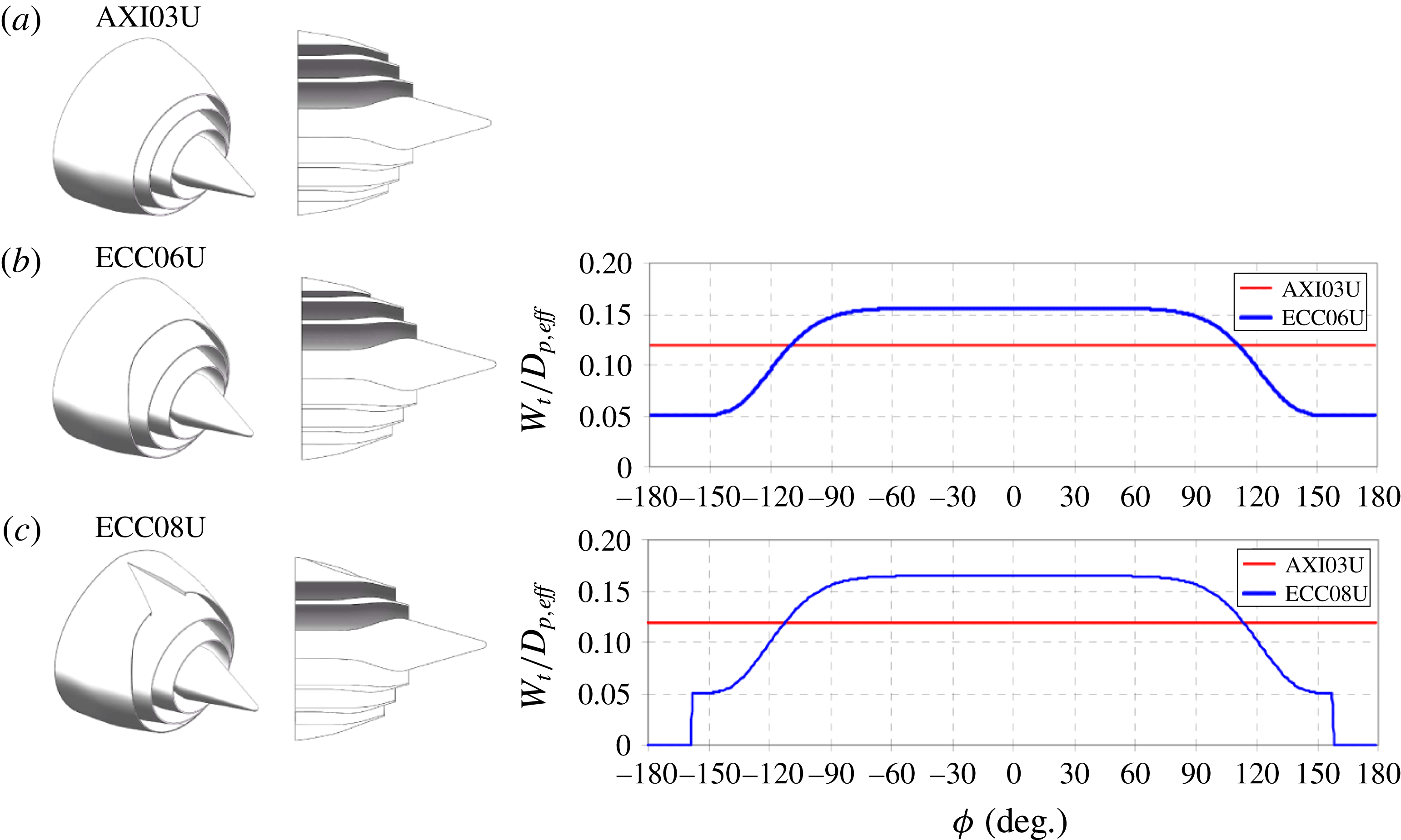
Figure 10. Three-stream nozzles with nominal plug. Left to right: perspective view, cross-sectional view and azimuthal distribution of the tertiary annulus width. Azimuthal angle
 $\unicode[STIX]{x1D719}$
is defined relative to the downward vertical direction.
$\unicode[STIX]{x1D719}$
is defined relative to the downward vertical direction.
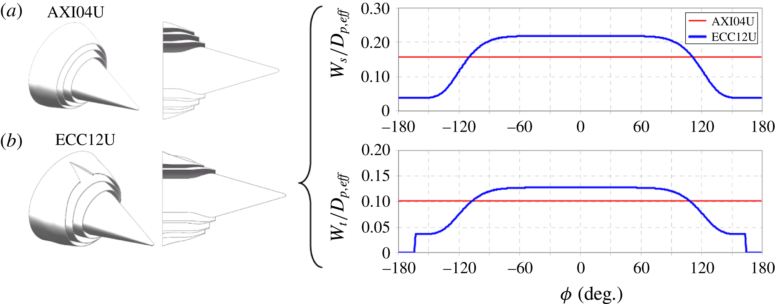
Figure 11. Three-stream nozzles with enlarged plug. Left to right: perspective view, cross-sectional view and azimuthal distributions of the widths of the secondary and tertiary annuli. Azimuthal angle
 $\unicode[STIX]{x1D719}$
is defined relative to the downward vertical direction.
$\unicode[STIX]{x1D719}$
is defined relative to the downward vertical direction.
The nozzles were tested at cycle conditions that were representative of three-stream turbofan engines operating at take-off power. Table 2 lists the main flow conditions at the nozzle exit. The Reynolds number of the primary stream, based on
 $D_{p,eff}$
, was 280 000. The exit velocities (
$D_{p,eff}$
, was 280 000. The exit velocities (
 $U$
) and Mach numbers (
$U$
) and Mach numbers (
 $M$
) were matched exactly using helium–air mixture jets (Papamoschou Reference Papamoschou2006).
$M$
) were matched exactly using helium–air mixture jets (Papamoschou Reference Papamoschou2006).
Table 2. Cycle point for three-stream jets.
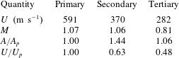
Noise measurements were conducted inside an anechoic chamber equipped with twenty-four 1/8-in. condenser microphones (Bruel & Kjaer, Model 4138) with frequency response up to 120 kHz. Twelve microphones were mounted on a downward arm (azimuth angle
 $\unicode[STIX]{x1D719}=0^{\circ }$
) and twelve were installed on a sideline arm (
$\unicode[STIX]{x1D719}=0^{\circ }$
) and twelve were installed on a sideline arm (
 $\unicode[STIX]{x1D719}=60^{\circ }$
). On each arm, the polar angle
$\unicode[STIX]{x1D719}=60^{\circ }$
). On each arm, the polar angle
 $\unicode[STIX]{x1D703}$
ranged approximately from
$\unicode[STIX]{x1D703}$
ranged approximately from
 $20$
to
$20$
to
 $120^{\circ }$
relative to the downstream jet axis, and the distance to the nozzle exit
$120^{\circ }$
relative to the downstream jet axis, and the distance to the nozzle exit
 ${\mathcal{R}}_{exp}$
ranges from 0.92 to 1.23 m. This arrangement enabled simultaneous measurement of the downward and sideline noise at all the polar angles of interest. In selected cases, rotation of the nozzle enabled a richer coverage of azimuthal angles. The microphones were connected, in groups of four, to six conditioning amplifiers (Bruel & Kjaer, Model 2690-A-0S4). The 24 outputs of the amplifiers were sampled simultaneously, at 250 kHz per channel, by three 8-channel multi-function data acquisition boards (National Instruments PCI-6143) installed in a Dell Precision T7400 computer with a Xeon quad-core processor. National Instruments LabView software is used to acquire the signals. The temperature and humidity inside the anechoic chamber are recorded to enable computation of the atmospheric absorption. The microphone signals were conditioned with a high-pass filter set at 300 Hz. Narrowband spectra were computed using a 4096-point fast Fourier transform, yielding a frequency resolution of 61 Hz. The spectra were corrected for microphone actuator response, microphone free field response and atmospheric absorption, thus resulting in lossless spectra.
${\mathcal{R}}_{exp}$
ranges from 0.92 to 1.23 m. This arrangement enabled simultaneous measurement of the downward and sideline noise at all the polar angles of interest. In selected cases, rotation of the nozzle enabled a richer coverage of azimuthal angles. The microphones were connected, in groups of four, to six conditioning amplifiers (Bruel & Kjaer, Model 2690-A-0S4). The 24 outputs of the amplifiers were sampled simultaneously, at 250 kHz per channel, by three 8-channel multi-function data acquisition boards (National Instruments PCI-6143) installed in a Dell Precision T7400 computer with a Xeon quad-core processor. National Instruments LabView software is used to acquire the signals. The temperature and humidity inside the anechoic chamber are recorded to enable computation of the atmospheric absorption. The microphone signals were conditioned with a high-pass filter set at 300 Hz. Narrowband spectra were computed using a 4096-point fast Fourier transform, yielding a frequency resolution of 61 Hz. The spectra were corrected for microphone actuator response, microphone free field response and atmospheric absorption, thus resulting in lossless spectra.
5.1.2 Acoustic results
Figure 12 plots narrowband SPL spectra in the downward direction (
 $\unicode[STIX]{x1D719}_{0}=0^{\circ }$
) for jets ECC06U and ECC08U, with comparison to AXI03U; and for jet ECC12U, with comparison to AXI04U. The spectra of the two reference coaxial jets, AXI03U (nominal plug) and AXI04U (enlarged plug), are very similar, with AXI04U having a 1–2 dB benefit at medium to high frequencies. This is partly attributed to source–observer shielding by the enlarged plug (Bauer, Kibens & Wlezien Reference Bauer, Kibens and Wlezien1982; Chase, Garzón & Papamoschou Reference Chase, Garzón and Papamoschou2013). Considering the nominal-plug asymmetric jets, ECC06U offers reductions of the order of 10 dB at polar angles near the angle of peak emission and in the medium to high frequency range. Addition of the wedge deflector in nozzle ECC08U increases these reductions to
$\unicode[STIX]{x1D719}_{0}=0^{\circ }$
) for jets ECC06U and ECC08U, with comparison to AXI03U; and for jet ECC12U, with comparison to AXI04U. The spectra of the two reference coaxial jets, AXI03U (nominal plug) and AXI04U (enlarged plug), are very similar, with AXI04U having a 1–2 dB benefit at medium to high frequencies. This is partly attributed to source–observer shielding by the enlarged plug (Bauer, Kibens & Wlezien Reference Bauer, Kibens and Wlezien1982; Chase, Garzón & Papamoschou Reference Chase, Garzón and Papamoschou2013). Considering the nominal-plug asymmetric jets, ECC06U offers reductions of the order of 10 dB at polar angles near the angle of peak emission and in the medium to high frequency range. Addition of the wedge deflector in nozzle ECC08U increases these reductions to
 ${\sim}$
15 dB. For the enlarged-plug asymmetric jet ECC12U, the combined asymmetry of the secondary and tertiary streams increases the noise reduction to
${\sim}$
15 dB. For the enlarged-plug asymmetric jet ECC12U, the combined asymmetry of the secondary and tertiary streams increases the noise reduction to
 ${\sim}17~\text{dB}$
. Change in noise emission in the broadside direction (
${\sim}17~\text{dB}$
. Change in noise emission in the broadside direction (
 $\unicode[STIX]{x1D703}\approx 90^{\circ }$
) is dependent on the aggressiveness of the asymmetry, with jets ECC06U and ECC08U showing a slight increase, and jet ECC12U causing a moderate increase. Spectra at different azimuthal angles will be presented later in the discussion of the model predictions. Considering the sideline direction
$\unicode[STIX]{x1D703}\approx 90^{\circ }$
) is dependent on the aggressiveness of the asymmetry, with jets ECC06U and ECC08U showing a slight increase, and jet ECC12U causing a moderate increase. Spectra at different azimuthal angles will be presented later in the discussion of the model predictions. Considering the sideline direction
 $\unicode[STIX]{x1D719}_{0}=60^{\circ }$
, jets ECC06U and ECC08U do not produce a significant benefit, while jet ECC12U provides a distinct reduction at low frequency.
$\unicode[STIX]{x1D719}_{0}=60^{\circ }$
, jets ECC06U and ECC08U do not produce a significant benefit, while jet ECC12U provides a distinct reduction at low frequency.
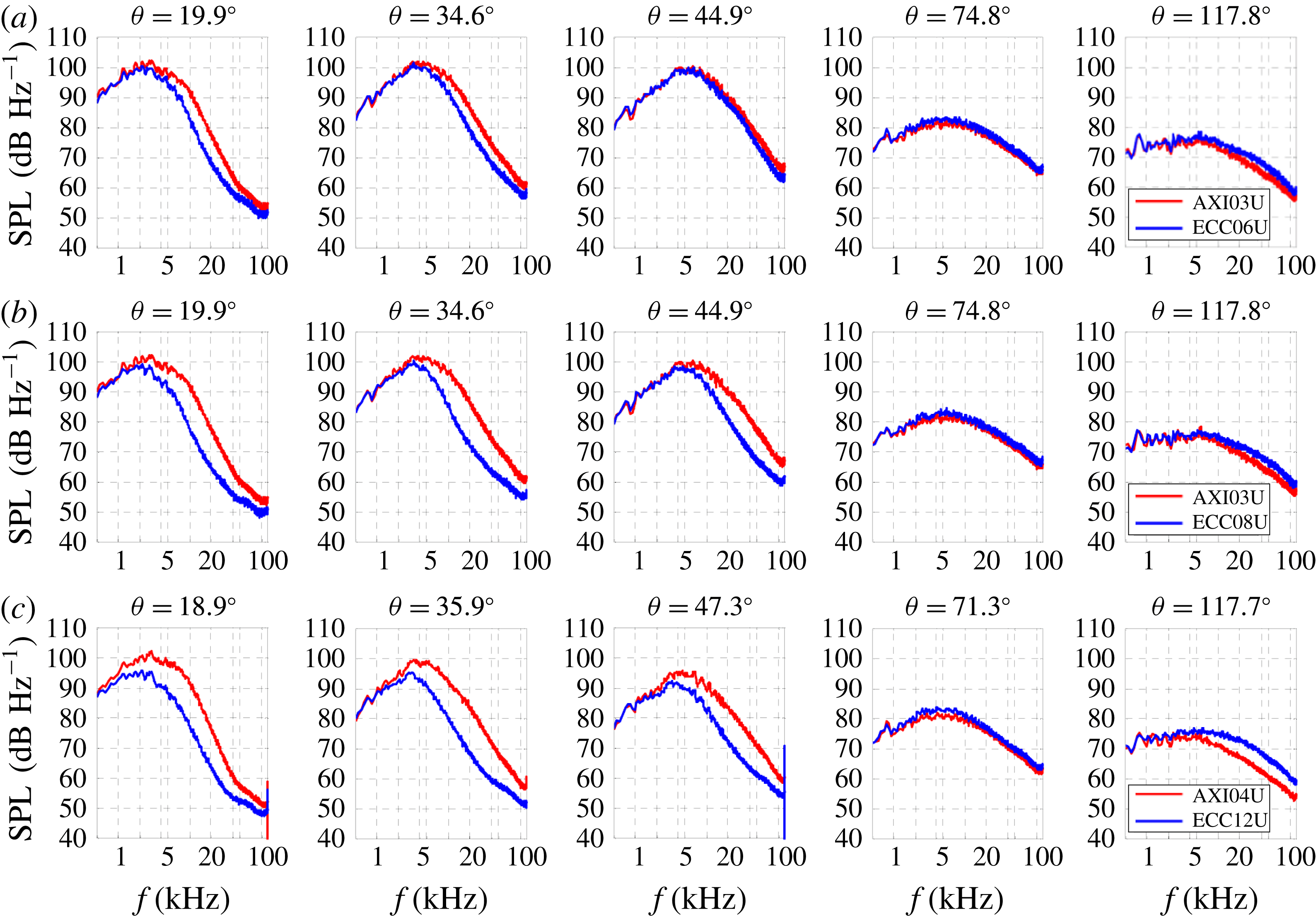
Figure 12. Narrowband far-field spectra at various polar angles
 $\unicode[STIX]{x1D703}$
for jets (a) ECC06U and (b) ECC08U, with comparison to reference jet AXI03U (red); and (c) jet ECC12U with comparison to reference jet AXI04U (red). Azimuthal direction
$\unicode[STIX]{x1D703}$
for jets (a) ECC06U and (b) ECC08U, with comparison to reference jet AXI03U (red); and (c) jet ECC12U with comparison to reference jet AXI04U (red). Azimuthal direction
 $\unicode[STIX]{x1D719}=0^{\circ }$
(downward).
$\unicode[STIX]{x1D719}=0^{\circ }$
(downward).
5.2 Computational
5.2.1 Code and grid
The computational fluid dynamics code used here is known as PARCAE (Papamoschou, Xiong & Liu Reference Papamoschou, Xiong and Liu2008) and solves the unsteady three-dimensional Navier–Stokes equations on structured multiblock grids using a cell-centred finite-volume method. Information exchange for flow computation on multiblock grids using multiple CPUs is implemented through the MPI (message passing interface) protocol. In its time-averaged implementation, the code solves the RANS equations using the Jameson–Schmidt–Turkel dissipation scheme (Jameson, Schmidt & Turkel Reference Jameson, Schmidt and Turkel1981) and the shear stress transport (SST) turbulence model (Menter Reference Menter1994). The SST model combines the advantages of the
 $k-\unicode[STIX]{x1D6FA}$
and
$k-\unicode[STIX]{x1D6FA}$
and
 $k-\unicode[STIX]{x1D716}$
turbulence models for both wall-bounded and free-stream flows.
$k-\unicode[STIX]{x1D716}$
turbulence models for both wall-bounded and free-stream flows.
The governing equations were solved explicitly in a coupled manner using five-stage Runge–Kutta scheme towards steady state with local time stepping, residual smoothing and multigrid techniques for convergence acceleration. Only the steady-state solution was considered because we are interested in the time-averaged features of the flow. The computation encompassed both the internal nozzle flow as well as the external plume. The computational domain extended to 38 tertiary nozzle diameters
 $D_{t}$
downstream and 8
$D_{t}$
downstream and 8
 $D_{t}$
radially. As all the configurations were symmetric about the meridian plane, only one half of the domain was modelled to save computational cost. The typical grid contained 8 million points. The grid was divided into multiblocks to implement parallelization on multiprocessor computers to reduce the convergence time. For the primary, secondary and tertiary duct flows, uniform total pressure was specified at the inlet surface corresponding to the perfectly expanded exit Mach number. For the ambient region surrounding the nozzle flow, a characteristic boundary condition was defined and the downstream static pressure was set equal to the ambient pressure. Adiabatic no-slip boundary condition was specified on all nozzle walls.
$D_{t}$
radially. As all the configurations were symmetric about the meridian plane, only one half of the domain was modelled to save computational cost. The typical grid contained 8 million points. The grid was divided into multiblocks to implement parallelization on multiprocessor computers to reduce the convergence time. For the primary, secondary and tertiary duct flows, uniform total pressure was specified at the inlet surface corresponding to the perfectly expanded exit Mach number. For the ambient region surrounding the nozzle flow, a characteristic boundary condition was defined and the downstream static pressure was set equal to the ambient pressure. Adiabatic no-slip boundary condition was specified on all nozzle walls.
The code has been used in past research on dual-stream symmetric and asymmetric jets, and its predictions have been validated against mean velocity measurements under cold conditions (Xiong et al. Reference Xiong, Nielsen, Liu and Papamoschou2010). Cold-flow comparisons for three-stream jets similar to those discussed here have shown similar level of agreement. In addition to providing information on the plume flow field, the code also predicts the aerodynamic performance of the nozzles. Here the code was applied at the conditions shown in table 1 and the experimental Reynolds numbers.
Using a filter based on the amplitude of the space–time correlation (3.45), computational elements with negligible impact on the spectral prediction were removed from the domain prior to running the acoustic analogy algorithms. This cut down the total number of elements to about two million, thus reducing significantly the computational cost. Additional cost-saving measures are discussed in appendix A.
5.2.2 Relevant statistics
For conciseness, the presentation of the RANS solutions will focus on the nominal-plug jets AXI03U, ECC06U and ECC08U. The trends delineated will apply broadly to the enlarged-plug jets AXI04U and ECC12U, and distinctions will be pointed out in § 5.2.3. The discussion starts with contour maps of the mean axial velocity on the symmetry (
 $X{-}Y$
) plane, shown in figure 13.
$X{-}Y$
) plane, shown in figure 13.
 $X=0$
signifies the location of the plug tip. For the axisymmetric jet AXI03U, the high-speed region extends to approximately seven tertiary diameters. The asymmetric delivery of the tertiary stream shortens moderately the high-speed region to
$X=0$
signifies the location of the plug tip. For the axisymmetric jet AXI03U, the high-speed region extends to approximately seven tertiary diameters. The asymmetric delivery of the tertiary stream shortens moderately the high-speed region to
 $x/D_{t}\approx 6.5$
for jet ECC06U and
$x/D_{t}\approx 6.5$
for jet ECC06U and
 $x/D_{t}\approx 6.0$
for jet ECC08U. For the asymmetric jets, the thickening of the low-speed flow on the underside of the jet is evident. Some distortion of the high-speed region is also noticeable. The plug wake is evident for all the jets.
$x/D_{t}\approx 6.0$
for jet ECC08U. For the asymmetric jets, the thickening of the low-speed flow on the underside of the jet is evident. Some distortion of the high-speed region is also noticeable. The plug wake is evident for all the jets.
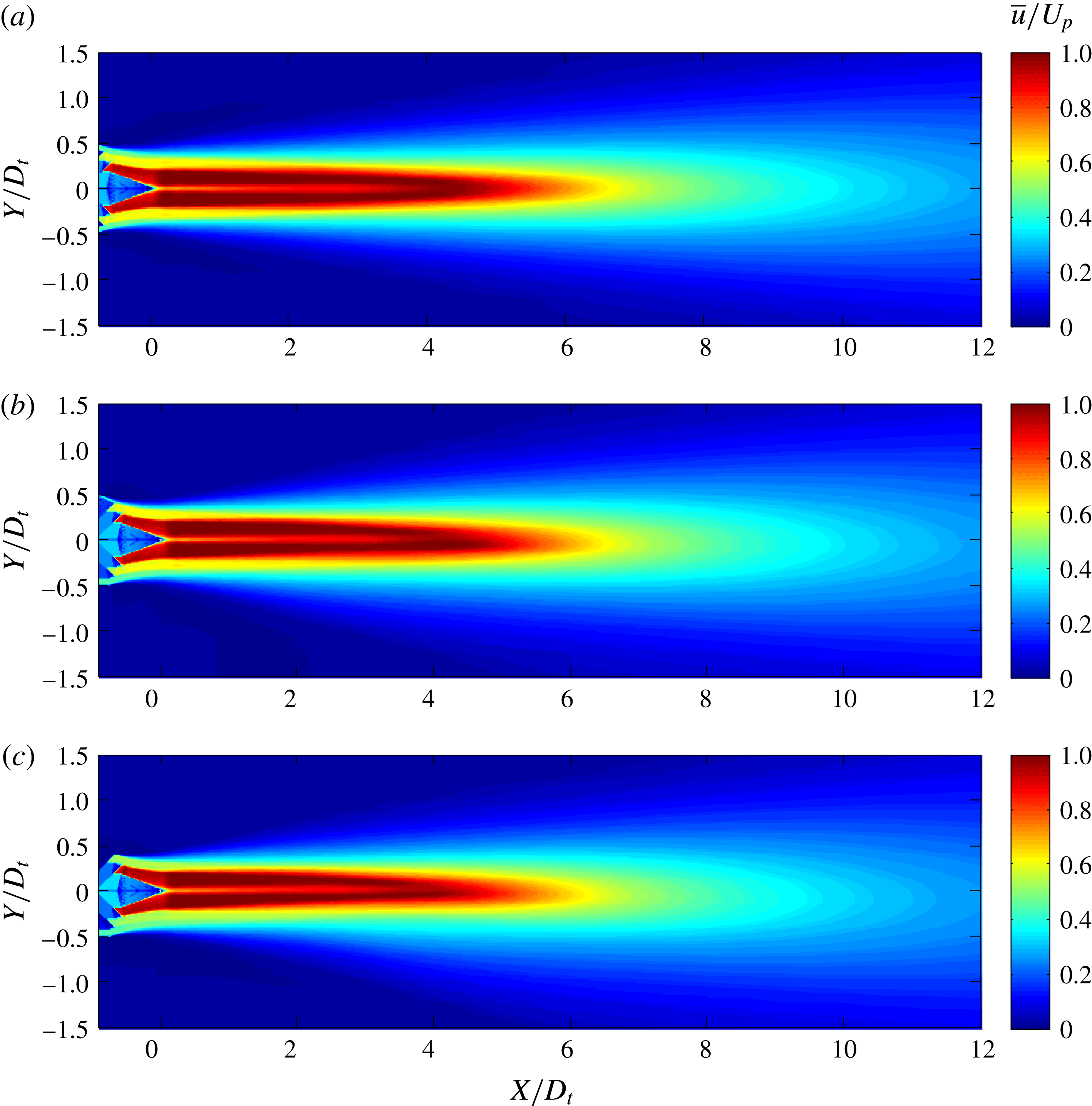
Figure 13. Distribution of normalized mean axial velocity
 $\overline{u}/U_{p}$
on the symmetry plane of jets: (a) AXI03U; (b) ECC06U; and (c) ECC08U.
$\overline{u}/U_{p}$
on the symmetry plane of jets: (a) AXI03U; (b) ECC06U; and (c) ECC08U.
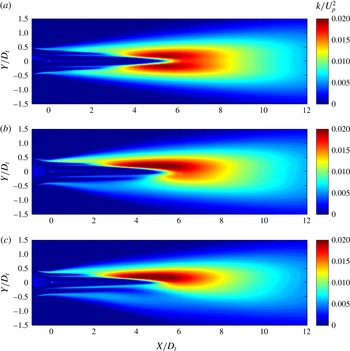
Figure 14. Distribution of normalized turbulent kinetic energy
 $k/U_{p}^{2}$
on the symmetry plane of jets: (a) AXI03U; (b) ECC06U; and (c) ECC08U.
$k/U_{p}^{2}$
on the symmetry plane of jets: (a) AXI03U; (b) ECC06U; and (c) ECC08U.
Figure 14 plots the corresponding distributions of the normalized turbulent kinetic energy
 $k/U_{p}^{2}$
. For jet AXI03U, in the vicinity of the nozzle exit we can distinguish clearly the outer shear layer (between the tertiary stream and the ambient) and the weaker inner shear layer (between the primary and secondary streams). The middle shear layer (between the secondary and tertiary streams) is not apparent. We gain an understanding of the relative strengths of the shear layers by considering that the turbulent kinetic energy (or any component of the Reynolds stress) scales approximately as
$k/U_{p}^{2}$
. For jet AXI03U, in the vicinity of the nozzle exit we can distinguish clearly the outer shear layer (between the tertiary stream and the ambient) and the weaker inner shear layer (between the primary and secondary streams). The middle shear layer (between the secondary and tertiary streams) is not apparent. We gain an understanding of the relative strengths of the shear layers by considering that the turbulent kinetic energy (or any component of the Reynolds stress) scales approximately as
 $(\unicode[STIX]{x0394}U)^{2}$
, where
$(\unicode[STIX]{x0394}U)^{2}$
, where
 $\unicode[STIX]{x0394}U$
is the velocity difference across a particular shear layer. It is insightful to assess the strengths in terms of the dimensionless ratio
$\unicode[STIX]{x0394}U$
is the velocity difference across a particular shear layer. It is insightful to assess the strengths in terms of the dimensionless ratio
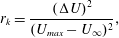 $$\begin{eqnarray}r_{k}=\frac{(\unicode[STIX]{x0394}U)^{2}}{(U_{max}-U_{\infty })^{2}},\end{eqnarray}$$
where the denominator signifies the largest possible strength, with
 $U_{max}$
the maximum fully expanded velocity (in this case, the primary exit velocity) and
$U_{max}$
the maximum fully expanded velocity (in this case, the primary exit velocity) and
 $U_{\infty }$
the ambient velocity (in this case, zero). From the values of table 2 we have
$U_{\infty }$
the ambient velocity (in this case, zero). From the values of table 2 we have
 $r_{k}=0.139$
, 0.022 and 0.228 for the inner, middle and outer shear layer, respectively. This dimensional argument helps explain the dominance of the outer shear layer and the near invisibility of the middle shear layer. At approximately
$r_{k}=0.139$
, 0.022 and 0.228 for the inner, middle and outer shear layer, respectively. This dimensional argument helps explain the dominance of the outer shear layer and the near invisibility of the middle shear layer. At approximately
 $x/D_{t}=2.5$
the secondary and tertiary streams are completely merged with primary shear layer. Now the primary eddies are in direct contact with the ambient, resulting in a rapid increase in the turbulent kinetic energy which reaches its maximum value near
$x/D_{t}=2.5$
the secondary and tertiary streams are completely merged with primary shear layer. Now the primary eddies are in direct contact with the ambient, resulting in a rapid increase in the turbulent kinetic energy which reaches its maximum value near
 $x/D_{t}=5.5$
. Here the ratio
$x/D_{t}=5.5$
. Here the ratio
 $r_{k}$
is close to unity. The location of peak turbulent kinetic energy is very close to the end of the primary potential core, as delineated by the cone-like region of very low turbulent intensity. Further downstream, the turbulent kinetic energy declines as the jet mean velocity drops. It is notable that at large downstream distances the profile for the turbulent kinetic energy becomes Gaussian-like.
$r_{k}$
is close to unity. The location of peak turbulent kinetic energy is very close to the end of the primary potential core, as delineated by the cone-like region of very low turbulent intensity. Further downstream, the turbulent kinetic energy declines as the jet mean velocity drops. It is notable that at large downstream distances the profile for the turbulent kinetic energy becomes Gaussian-like.
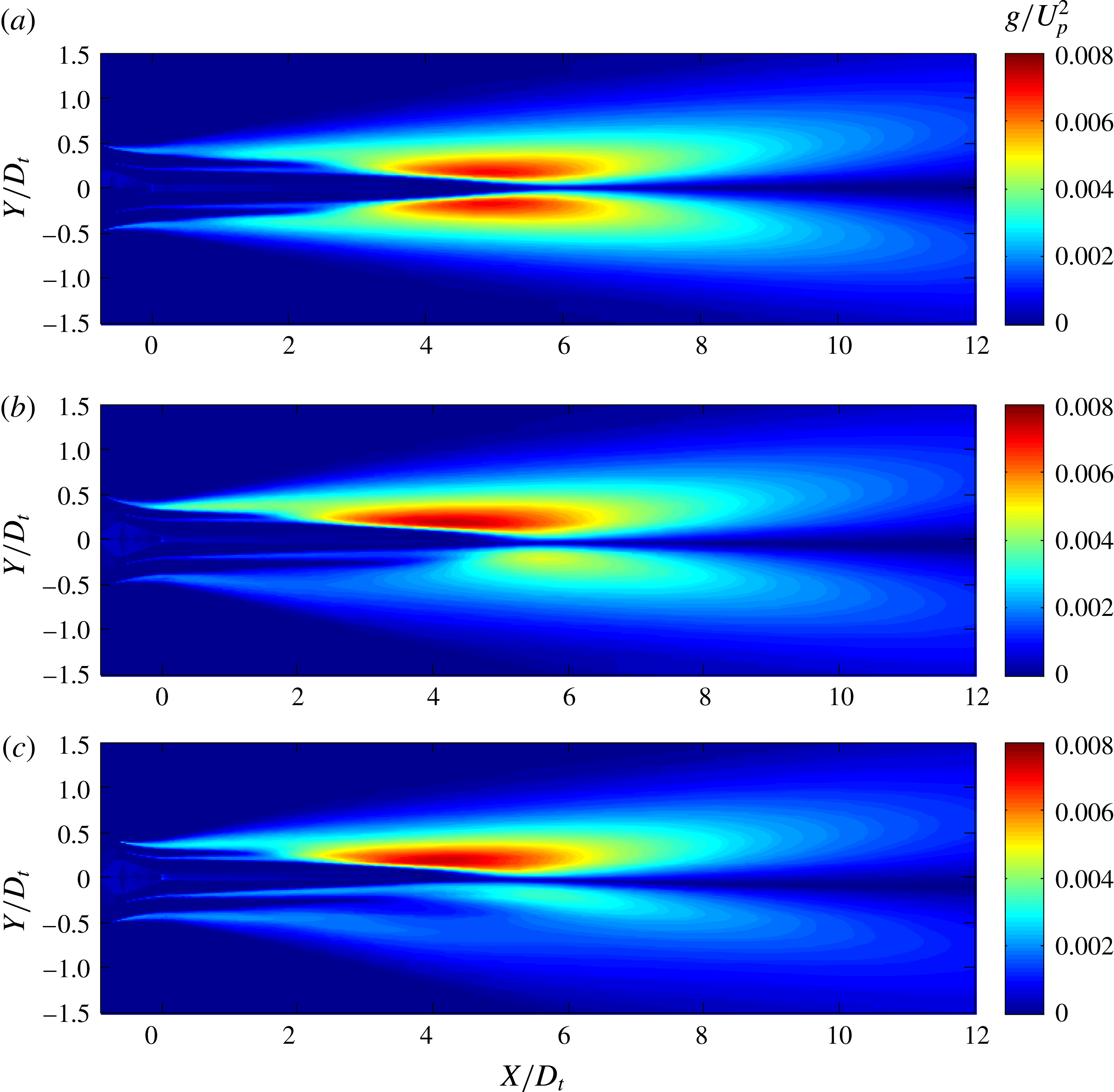
Figure 15. Distribution of normalized Reynolds stress
 $g/U_{p}^{2}$
on the symmetry plane of jets: (a) AXI03U; (b) ECC06U; and (c) ECC08U. Compare with the distribution of the turbulent kinetic energy in figure 14, particularly past
$g/U_{p}^{2}$
on the symmetry plane of jets: (a) AXI03U; (b) ECC06U; and (c) ECC08U. Compare with the distribution of the turbulent kinetic energy in figure 14, particularly past
 $x/D_{t}=5$
.
$x/D_{t}=5$
.
For the asymmetric jets ECC06U and ECC08U the secondary and tertiary streams extend much longer on the underside of the jet, reaching
 $x/D_{t}=4$
for ECC06U and
$x/D_{t}=4$
for ECC06U and
 $x/D_{t}=5$
for ECC08U. Their elongation prevents the contact of the primary eddies with the ambient until past the end of the primary core. As a result, the turbulent kinetic energy on the underside of the jet is significantly reduced; this effect is most pronounced for jet ECC08U. The primary potential core is moderately reduced to
$x/D_{t}=5$
for ECC08U. Their elongation prevents the contact of the primary eddies with the ambient until past the end of the primary core. As a result, the turbulent kinetic energy on the underside of the jet is significantly reduced; this effect is most pronounced for jet ECC08U. The primary potential core is moderately reduced to
 $x/D_{t}=5.2$
for ECC06U and
$x/D_{t}=5.2$
for ECC06U and
 $x/D_{t}=4.8$
for ECC08U. All these trends bode well for noise reduction in the downward direction. However, looking at the distributions of figure 14(b,c) one has difficulty drawing a line distinguishing unambiguously the upper and lower sides of the jet.
$x/D_{t}=4.8$
for ECC08U. All these trends bode well for noise reduction in the downward direction. However, looking at the distributions of figure 14(b,c) one has difficulty drawing a line distinguishing unambiguously the upper and lower sides of the jet.
We turn our attention to the distribution of the normalized ‘Reynolds stress’
 $g/U_{p}^{2}$
, depicted in figure 15. The distribution of
$g/U_{p}^{2}$
, depicted in figure 15. The distribution of
 $g$
near the nozzle exit is very similar to that of
$g$
near the nozzle exit is very similar to that of
 $k$
, so the same arguments apply there. However, further downstream we note a significant difference between the
$k$
, so the same arguments apply there. However, further downstream we note a significant difference between the
 $g$
and
$g$
and
 $k$
fields. The
$k$
fields. The
 $g$
field has a clear minimum in the interior of the jet, which is practically zero once the wake region dissipates. The location of the minimum coincides with the jet centroid defined by (3.13). Downstream of the end of the potential core, the distribution of
$g$
field has a clear minimum in the interior of the jet, which is practically zero once the wake region dissipates. The location of the minimum coincides with the jet centroid defined by (3.13). Downstream of the end of the potential core, the distribution of
 $g$
has two lobes representing the turbulence production near the edge of the jet. Compare with the Gaussian-like profile for
$g$
has two lobes representing the turbulence production near the edge of the jet. Compare with the Gaussian-like profile for
 $k$
in figure 14. We can clearly delineate the upper and lower sides of the jet, as demarcated by the location of the minimum
$k$
in figure 14. We can clearly delineate the upper and lower sides of the jet, as demarcated by the location of the minimum
 $g$
. The lower side experiences dramatic reductions in
$g$
. The lower side experiences dramatic reductions in
 $g$
, particularly in jet ECC08U. These results reinforce the view discussed in § 2.1 that the Reynolds stress is the appropriate statistical quantity to represent the action of the turbulent eddies.
$g$
, particularly in jet ECC08U. These results reinforce the view discussed in § 2.1 that the Reynolds stress is the appropriate statistical quantity to represent the action of the turbulent eddies.
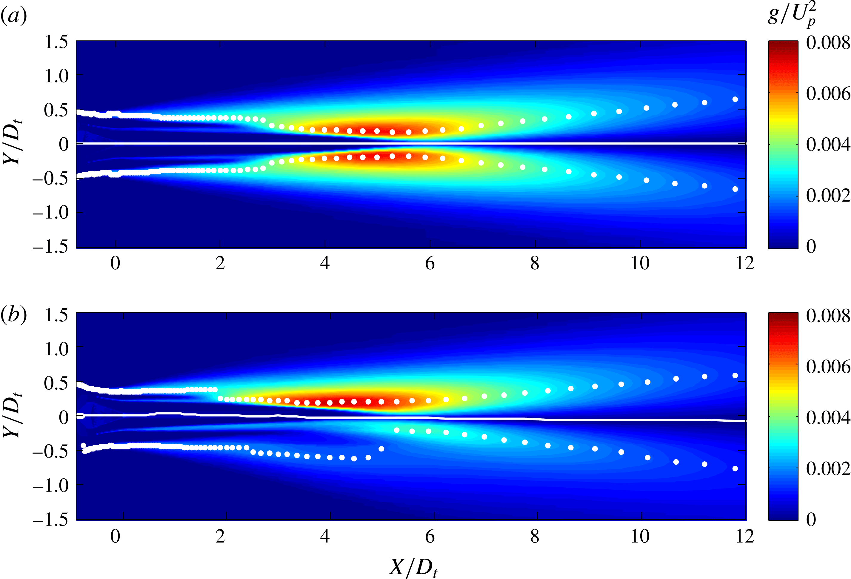
Figure 16. Location of the outer surface of peak stress (OSPS) on the symmetry plane of jets (a) AXI03U and (b) ECC08U. Contour map shows the Reynolds stress field
 $g/U_{p}^{2}$
. White dots indicate the location of the outermost peak of
$g/U_{p}^{2}$
. White dots indicate the location of the outermost peak of
 $g$
. Solid white line is the jet centroid as defined by (3.13).
$g$
. Solid white line is the jet centroid as defined by (3.13).
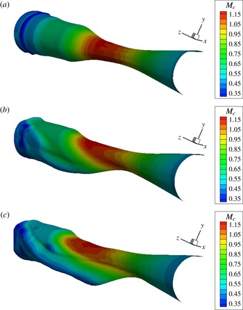
Figure 17. Outer surface of peak stress (OSPS) for jets (a) AXI03U, (b) ECC06U and (c) ECC08U. Contour levels show distribution of
 $M_{c}$
on the OSPS.
$M_{c}$
on the OSPS.
5.2.3 OSPS
We now examine the geometry of the outer surface of peak stress. Figure 16 plots the location of the OSPS on the symmetry plane of jets AXI03U and ECC08U. The plots of the OSPS are overlaid on contour maps of the Reynolds stress
 $g$
. For the axisymmetric jet, the OSPS experiences a sudden convergence where the outer streams become totally mixed with the primary shear later, near
$g$
. For the axisymmetric jet, the OSPS experiences a sudden convergence where the outer streams become totally mixed with the primary shear later, near
 $x/D_{t}=2.5$
. This is followed by a gradual convergence near the end of the primary potential core, downstream of which the OSPS diverges slowly. For the asymmetric jet, the OSPS on the top side of the jet is similar to that for the axisymmetric jet. On the bottom side, the OSPS slightly diverges in the initial region of the jet, then suddenly shifts inward near
$x/D_{t}=2.5$
. This is followed by a gradual convergence near the end of the primary potential core, downstream of which the OSPS diverges slowly. For the asymmetric jet, the OSPS on the top side of the jet is similar to that for the axisymmetric jet. On the bottom side, the OSPS slightly diverges in the initial region of the jet, then suddenly shifts inward near
 $x/D_{t}=5$
, the location where the outer streams are totally mixed with the primary stream. For the first five diameters or so the OSPS on the bottom side is in a low velocity region of the jet, meaning that the convective Mach number there is low subsonic. This has a large impact on the prediction of noise emission from this region. Figure 16 also depicts the location of the centroid, which is seen to coincide with the locus of minimum Reynolds stress.
$x/D_{t}=5$
, the location where the outer streams are totally mixed with the primary stream. For the first five diameters or so the OSPS on the bottom side is in a low velocity region of the jet, meaning that the convective Mach number there is low subsonic. This has a large impact on the prediction of noise emission from this region. Figure 16 also depicts the location of the centroid, which is seen to coincide with the locus of minimum Reynolds stress.
We gain further insight by examining three-dimensional views of the OSPS, plotted in figure 17. The distribution of the convective Mach number
 $M_{c}$
is shown as contour levels on the surfaces. The views cover the axial range
$M_{c}$
is shown as contour levels on the surfaces. The views cover the axial range
 $-0.5\leqslant x/D_{t}\leqslant 10$
. For jet AXI03U, the transition of the OSPS from the tertiary to the secondary to the primary shear layer is evident. The convective Mach number reaches the peak value of 1.20 shortly downstream of the transition to the primary shear layer. For jets ECC06U and ECC08U we observe a progressively stronger reshaping of the OSPS, starting at the lateral sides and progressing to the lower side. For jet ECC08U, on the underside of the OSPS, the convective Mach number is as low as 0.35. This corresponds to of the order of a 100-fold reduction in radiation efficiency in that region, as will be explained in § 7. On the upper half of the jet, the shape of the OSPS and the
$-0.5\leqslant x/D_{t}\leqslant 10$
. For jet AXI03U, the transition of the OSPS from the tertiary to the secondary to the primary shear layer is evident. The convective Mach number reaches the peak value of 1.20 shortly downstream of the transition to the primary shear layer. For jets ECC06U and ECC08U we observe a progressively stronger reshaping of the OSPS, starting at the lateral sides and progressing to the lower side. For jet ECC08U, on the underside of the OSPS, the convective Mach number is as low as 0.35. This corresponds to of the order of a 100-fold reduction in radiation efficiency in that region, as will be explained in § 7. On the upper half of the jet, the shape of the OSPS and the
 $M_{c}$
distributions are similar to those of the axisymmetric case.
$M_{c}$
distributions are similar to those of the axisymmetric case.
For completeness we also examine the OSPS of the enlarged-plug jets AXI04U and ECC12U in figure 18. For jet AXI04U, the shape of the OSPS and
 $M_{c}$
distribution on it are similar to those of jet AXI03U. However, jet ECC12U shows a more distorted OSPS relative to ECC06U or ECC08U, a result of the combined asymmetry of the secondary and tertiary ducts. The secondary and tertiary flows are more evenly distributed on the underside of the jet, which suggests that this jet may have better sideline noise reduction than ECC06U or ECC08U.
$M_{c}$
distribution on it are similar to those of jet AXI03U. However, jet ECC12U shows a more distorted OSPS relative to ECC06U or ECC08U, a result of the combined asymmetry of the secondary and tertiary ducts. The secondary and tertiary flows are more evenly distributed on the underside of the jet, which suggests that this jet may have better sideline noise reduction than ECC06U or ECC08U.
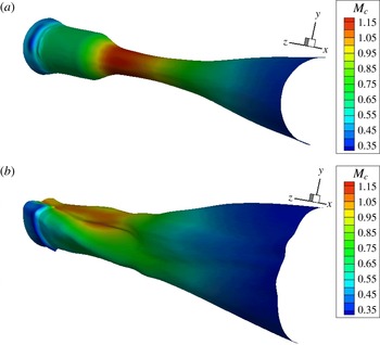
Figure 18. Outer surface of peak stress (OSPS) for jets (a) AXI04U and (b) ECC12U. Contour levels show distribution of
 $M_{c}$
on the OSPS.
$M_{c}$
on the OSPS.
It is also instructive to examine the distribution of
 $M_{c}$
versus axial and azimuthal directions, as is done in figure 19 for the nominal-plug jets. The largest reduction in
$M_{c}$
versus axial and azimuthal directions, as is done in figure 19 for the nominal-plug jets. The largest reduction in
 $M_{c}$
occurs in the downward direction
$M_{c}$
occurs in the downward direction
 $\unicode[STIX]{x1D719}=0$
. There the peak value of
$\unicode[STIX]{x1D719}=0$
. There the peak value of
 $M_{c}$
reduces from 1.2 for AXI03U to 1.0 for ECC06U to 0.8 for ECC08U. It is also noted that the distribution of the peak becomes confined to only about one diameter for ECC08U, versus three diameters for AXI03U. For ECC08U, the low-
$M_{c}$
reduces from 1.2 for AXI03U to 1.0 for ECC06U to 0.8 for ECC08U. It is also noted that the distribution of the peak becomes confined to only about one diameter for ECC08U, versus three diameters for AXI03U. For ECC08U, the low-
 $M_{c}$
region persists up to about
$M_{c}$
region persists up to about
 $\unicode[STIX]{x1D719}=50^{\circ }$
, after which the distribution becomes similar to that of the axisymmetric jet. The significant improvement in suppression of convective Mach number in jet ECC08U, versus jet ECC06U, came from a rather subtle reshaping of the tertiary duct, as illustrated in figure 10. This underscores the sensitivity of the offset-stream method to the fine details of the duct reshaping. The convective Mach number distribution for jet ECC12U, plotted in figure 20, shows a large suppression of
$\unicode[STIX]{x1D719}=50^{\circ }$
, after which the distribution becomes similar to that of the axisymmetric jet. The significant improvement in suppression of convective Mach number in jet ECC08U, versus jet ECC06U, came from a rather subtle reshaping of the tertiary duct, as illustrated in figure 10. This underscores the sensitivity of the offset-stream method to the fine details of the duct reshaping. The convective Mach number distribution for jet ECC12U, plotted in figure 20, shows a large suppression of
 $M_{c}$
extending up to
$M_{c}$
extending up to
 $\unicode[STIX]{x1D719}=40^{\circ }$
. It is evident that the combined asymmetry of the secondary and tertiary streams results in a wider azimuthal sector with low
$\unicode[STIX]{x1D719}=40^{\circ }$
. It is evident that the combined asymmetry of the secondary and tertiary streams results in a wider azimuthal sector with low
 $M_{c}$
.
$M_{c}$
.
The information presented in figures 17–20 constitutes important feedback one obtains from the RANS solution before proceeding to the acoustic analogy step. Examinations of the OSPS and the associated
 $M_{c}$
distribution provide strong clues whether a particular nozzle arrangement will produce a quiet jet and in what azimuthal directions. In the particular examples shown here, one can expect jet ECC08U to bring significant noise benefit in the downward direction but probably little or no benefit in the sideline direction, near
$M_{c}$
distribution provide strong clues whether a particular nozzle arrangement will produce a quiet jet and in what azimuthal directions. In the particular examples shown here, one can expect jet ECC08U to bring significant noise benefit in the downward direction but probably little or no benefit in the sideline direction, near
 $\unicode[STIX]{x1D719}_{0}=60^{\circ }$
. On the other hand, jet ECC12U may be expected to provide a strong downward reduction combined with a distinct, but not as large, sideline reduction.
$\unicode[STIX]{x1D719}_{0}=60^{\circ }$
. On the other hand, jet ECC12U may be expected to provide a strong downward reduction combined with a distinct, but not as large, sideline reduction.
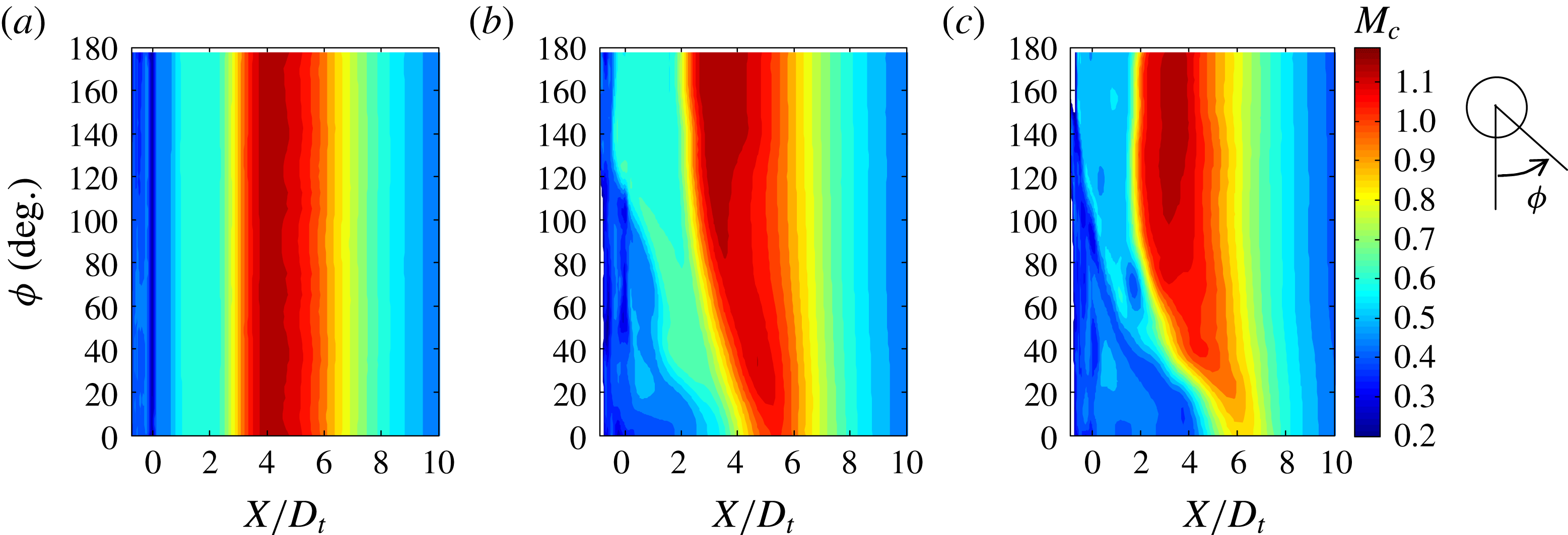
Figure 19. Axial–azimuthal distribution of convective Mach number
 $M_{c}$
on the OSPS of jets AXI03U (a), ECC06U (b) and ECC08U (c).
$M_{c}$
on the OSPS of jets AXI03U (a), ECC06U (b) and ECC08U (c).
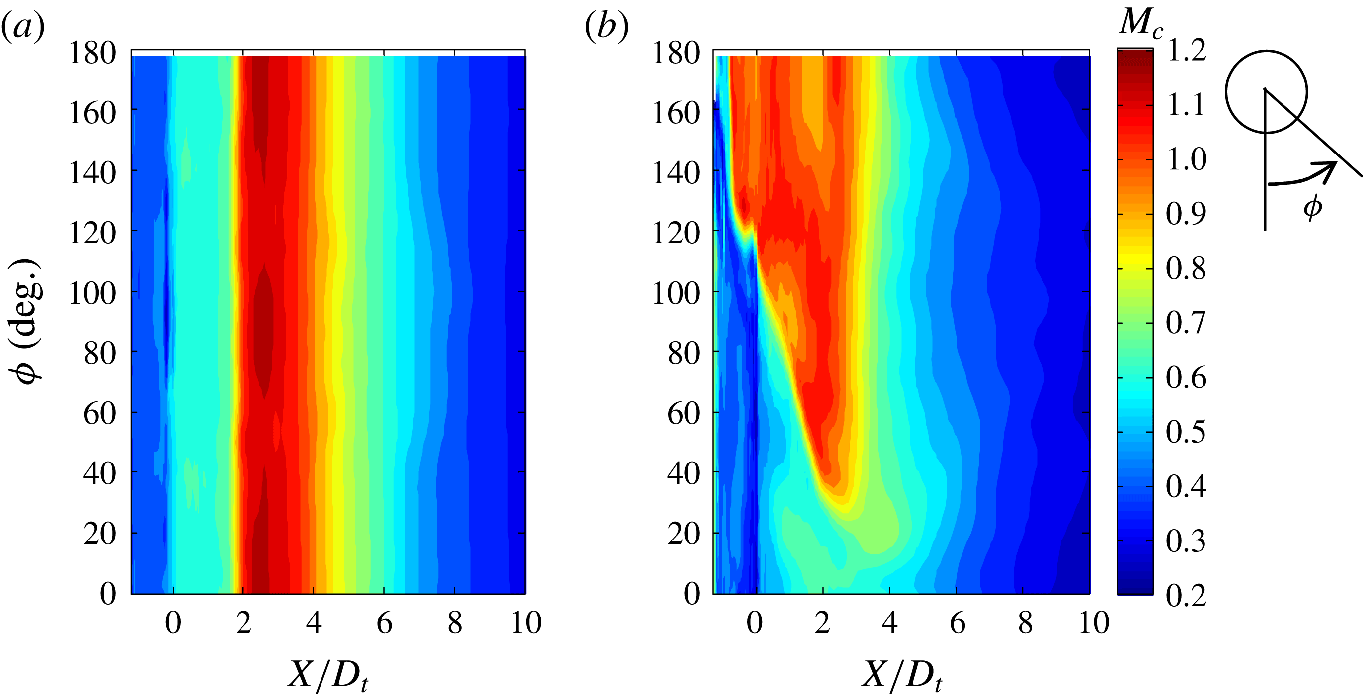
Figure 20. Axial–azimuthal distribution of convective Mach number
 $M_{c}$
on the OSPS of jets AXI04U (a) and ECC12U (b).
$M_{c}$
on the OSPS of jets AXI04U (a) and ECC12U (b).
6 Results
This study has introduced several new elements in the acoustic analogy modelling of peak noise from high-speed turbulent jets including: a broader class of functions for expressing the space–time correlation; definition of convective Mach number based on the locus of peak Reynolds stress; and azimuthal directivity formulation based on a transverse space–time correlation. This section discusses representative results of this modelling effort, with application to the jets reviewed in § 5. All the results shown are in the direction of peak emission
 $\unicode[STIX]{x1D703}_{0}=35^{\circ }$
. The transverse convective Mach number was selected to be
$\unicode[STIX]{x1D703}_{0}=35^{\circ }$
. The transverse convective Mach number was selected to be
 $\unicode[STIX]{x1D707}_{c}=1.52$
consistently with (3.34).
$\unicode[STIX]{x1D707}_{c}=1.52$
consistently with (3.34).
In the discussion of the sound pressure level spectra, the frequency will be presented in the non-dimensional (Strouhal number) form
 $$\begin{eqnarray}S_{r}=\frac{fD_{t}}{U_{p}}=\frac{\unicode[STIX]{x1D714}D_{t}}{2\unicode[STIX]{x03C0}U_{p}}.\end{eqnarray}$$
This compound version of the Strouhal number tries to account for the overall diameter of the jet, which is largely controlled by diameter of the tertiary duct, and the maximum velocity of the flow.
Application of the conjugate-gradient method outlined in § 4.2, with
 $\unicode[STIX]{x1D6FD}_{23}=2$
, resulted in the parameter vectors, for the reference jets AXI03U and AXI04U, listed in table 3. The vectors for the two jets are similar, with AXI04U having moderately higher scale coefficients. A sensitivity analysis indicated that all five of the parameters are influential on the prediction of the modelled spectral density. Denoting
$\unicode[STIX]{x1D6FD}_{23}=2$
, resulted in the parameter vectors, for the reference jets AXI03U and AXI04U, listed in table 3. The vectors for the two jets are similar, with AXI04U having moderately higher scale coefficients. A sensitivity analysis indicated that all five of the parameters are influential on the prediction of the modelled spectral density. Denoting
 $\unicode[STIX]{x0394}\text{SPL}$
the root-mean-square deviation of the modelled spectral density from a nominal distribution (using a formulation similar to (4.5), but without the penalty component), the magnitudes of the derivatives
$\unicode[STIX]{x0394}\text{SPL}$
the root-mean-square deviation of the modelled spectral density from a nominal distribution (using a formulation similar to (4.5), but without the penalty component), the magnitudes of the derivatives
 $\unicode[STIX]{x2202}\unicode[STIX]{x0394}\text{SPL}/\unicode[STIX]{x2202}V_{k}$
are of the order of 10 to 100, depending on the value of the parameter vector
$\unicode[STIX]{x2202}\unicode[STIX]{x0394}\text{SPL}/\unicode[STIX]{x2202}V_{k}$
are of the order of 10 to 100, depending on the value of the parameter vector
 $\boldsymbol{V}$
. The sensitivity on the powers
$\boldsymbol{V}$
. The sensitivity on the powers
 $\unicode[STIX]{x1D6FD}_{1}$
and
$\unicode[STIX]{x1D6FD}_{1}$
and
 $\unicode[STIX]{x1D6FD}_{4}$
is typically very strong, as can be gleaned from figure 4, but the scale coefficients
$\unicode[STIX]{x1D6FD}_{4}$
is typically very strong, as can be gleaned from figure 4, but the scale coefficients
 $C_{1}$
,
$C_{1}$
,
 $C_{23}$
, and
$C_{23}$
, and
 $C_{4}$
are impactful as well.
$C_{4}$
are impactful as well.
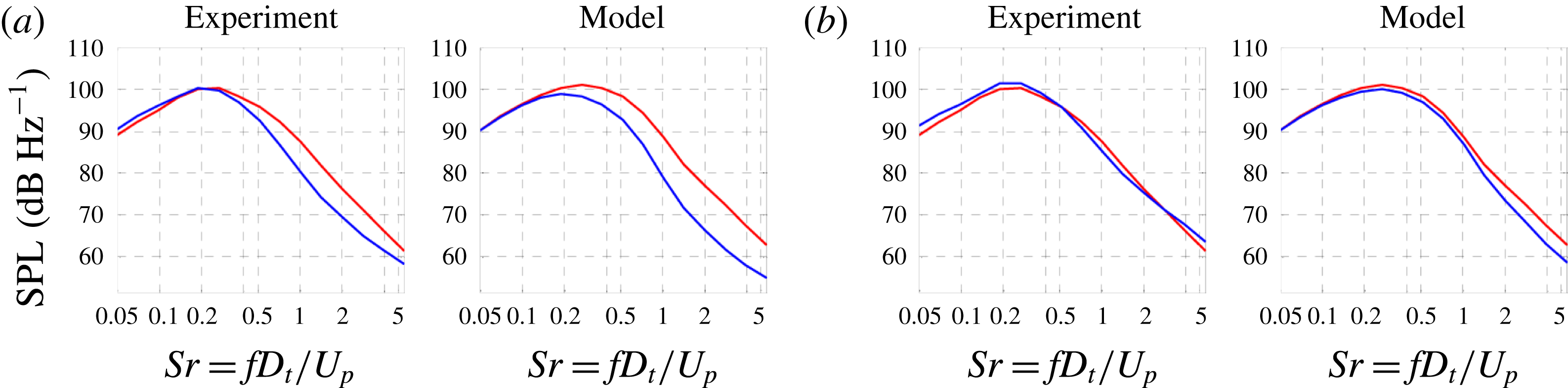
Figure 21. Experimental and modelled spectra for jets AXI03U (red) and ECC06U (blue) at polar angle
 $\unicode[STIX]{x1D703}_{0}=35^{\circ }$
. (a)
$\unicode[STIX]{x1D703}_{0}=35^{\circ }$
. (a)
 $\unicode[STIX]{x1D719}_{0}=0^{\circ }$
; (b)
$\unicode[STIX]{x1D719}_{0}=0^{\circ }$
; (b)
 $\unicode[STIX]{x1D719}_{0}=60^{\circ }$
.
$\unicode[STIX]{x1D719}_{0}=60^{\circ }$
.
Table 3. Parameter vectors for the reference jets.
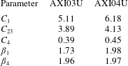
Figure 21 plots the experimental and modelled spectra for jets AXI03U (reference) and ECC06U at observer azimuthal angles
 $\unicode[STIX]{x1D719}_{0}=0^{\circ }$
(downward) and
$\unicode[STIX]{x1D719}_{0}=0^{\circ }$
(downward) and
 $\unicode[STIX]{x1D719}_{0}=60^{\circ }$
(sideline). First we note the excellent match for the reference spectra; as mentioned in § 4.2, the standard error is around 1.0 dB. In the downward direction, the model predicts the noise reduction accurately up to
$\unicode[STIX]{x1D719}_{0}=60^{\circ }$
(sideline). First we note the excellent match for the reference spectra; as mentioned in § 4.2, the standard error is around 1.0 dB. In the downward direction, the model predicts the noise reduction accurately up to
 $S_{r}\approx 2$
, with a small overprediction at higher Strouhal numbers. In the sideline direction, the model indicates marginal noise reduction, which is in line with the experiment.
$S_{r}\approx 2$
, with a small overprediction at higher Strouhal numbers. In the sideline direction, the model indicates marginal noise reduction, which is in line with the experiment.
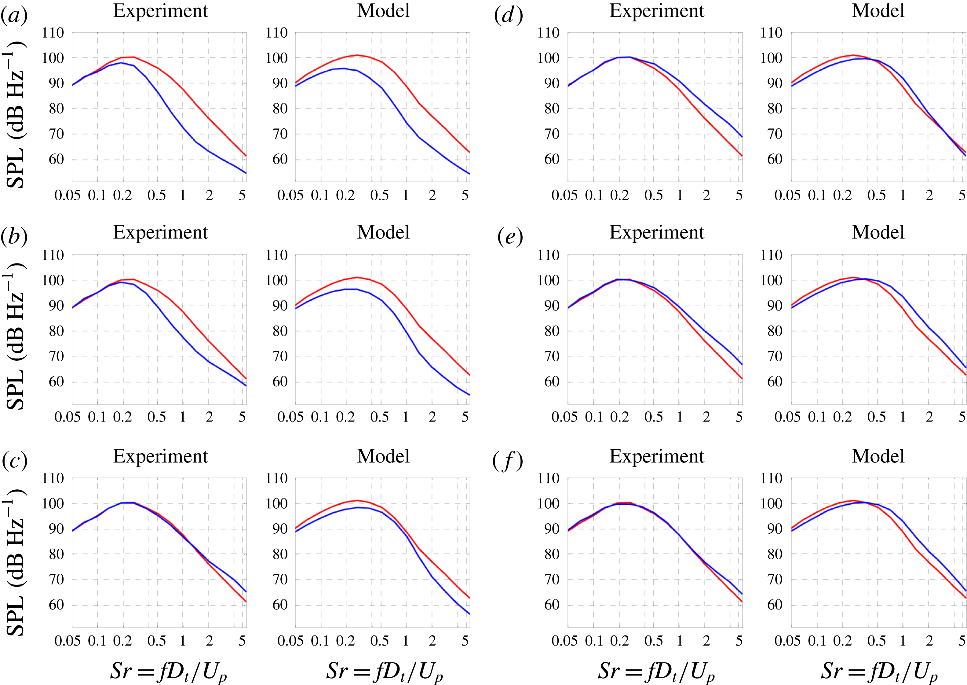
Figure 22. Experimental and modelled spectra for jets AXI03U (red) and ECC08U (blue) at polar angle
 $\unicode[STIX]{x1D703}_{0}=35^{\circ }$
. (a)
$\unicode[STIX]{x1D703}_{0}=35^{\circ }$
. (a)
 $\unicode[STIX]{x1D719}_{0}=0^{\circ }$
; (b)
$\unicode[STIX]{x1D719}_{0}=0^{\circ }$
; (b)
 $\unicode[STIX]{x1D719}_{0}=30^{\circ }$
; (c)
$\unicode[STIX]{x1D719}_{0}=30^{\circ }$
; (c)
 $\unicode[STIX]{x1D719}_{0}=60^{\circ }$
; (d)
$\unicode[STIX]{x1D719}_{0}=60^{\circ }$
; (d)
 $\unicode[STIX]{x1D719}_{0}=90^{\circ }$
; (e)
$\unicode[STIX]{x1D719}_{0}=90^{\circ }$
; (e)
 $\unicode[STIX]{x1D719}_{0}=135^{\circ }$
; and (f)
$\unicode[STIX]{x1D719}_{0}=135^{\circ }$
; and (f)
 $\unicode[STIX]{x1D719}_{0}=180^{\circ }$
.
$\unicode[STIX]{x1D719}_{0}=180^{\circ }$
.
Similar information is displayed for jet ECC08U in figure 22. The acoustics of this jet were surveyed at a larger set of azimuthal angles, ranging from
 $\unicode[STIX]{x1D719}_{0}=0^{\circ }$
(downward) to
$\unicode[STIX]{x1D719}_{0}=0^{\circ }$
(downward) to
 $\unicode[STIX]{x1D719}_{0}=180^{\circ }$
(upward). The larger downward noise reduction of jet ECC08U is captured well by the model, as are the trends with increasing azimuthal angle. For
$\unicode[STIX]{x1D719}_{0}=180^{\circ }$
(upward). The larger downward noise reduction of jet ECC08U is captured well by the model, as are the trends with increasing azimuthal angle. For
 $\unicode[STIX]{x1D719}_{0}>60^{\circ }$
, the experiment indicates moderate noise increase, which is generally reproduced by the model. Jet ECC12U was likewise surveyed at a number of azimuthal angles. The spectra plotted in figure 23 show that the model captures the principal noise trends, albeit with some overprediction of the noise reduction at low frequency. These trends include better reduction at a larger downward sector (
$\unicode[STIX]{x1D719}_{0}>60^{\circ }$
, the experiment indicates moderate noise increase, which is generally reproduced by the model. Jet ECC12U was likewise surveyed at a number of azimuthal angles. The spectra plotted in figure 23 show that the model captures the principal noise trends, albeit with some overprediction of the noise reduction at low frequency. These trends include better reduction at a larger downward sector (
 $0^{\circ }\leqslant \unicode[STIX]{x1D719}_{0}\leqslant 60^{\circ }$
) and stronger excess noise in the upward direction
$0^{\circ }\leqslant \unicode[STIX]{x1D719}_{0}\leqslant 60^{\circ }$
) and stronger excess noise in the upward direction
 $\unicode[STIX]{x1D719}_{0}=180^{\circ }$
. In particular, comparing figures 22(c) and 23(c) we note that the model indicates that ECC12U provides better sideline reduction than ECC08U, which is generally confirmed by the experiment.
$\unicode[STIX]{x1D719}_{0}=180^{\circ }$
. In particular, comparing figures 22(c) and 23(c) we note that the model indicates that ECC12U provides better sideline reduction than ECC08U, which is generally confirmed by the experiment.
The results of figures 22 and 23 can be summarized in the form of the change in overall sound pressure level (OASPL) versus azimuthal angle. The OASPL was computed by integrating versus frequency the modelled and experimental spectra. It is presented in two forms, the unweighted version and the A-weighted version. The A-weighted version accounts for the human perception of sound and is based on a scale factor of 40, representing the typical engine size for a supersonic business jet. For the A-weighted version, the SPL spectra were scaled up and ‘corrected’ with the A weight, using the formula in the ANSI S1.43 standard (Rimmell, Mansfield & Paddan Reference Rimmell, Mansfield and Paddan2015). The plots of
 $\unicode[STIX]{x0394}\text{OASPL}$
are shown in figures 24 and 25 for jets ECC08U and ECC12U, respectively. It is seen that the model captures the azimuthal variation of the noise. For the unweighted OASPL, the model overpredicts the reduction by approximately 2 dB in the downward direction. The agreement is better for the A-weighted OASPL because it is strongly influenced by the mid-frequencies where the model generally performs well. Comparing figures 24(b) and 25(b), the model predicts the superiority of nozzle ECC12U in suppressing downward noise as well as providing better sideline reduction.
$\unicode[STIX]{x0394}\text{OASPL}$
are shown in figures 24 and 25 for jets ECC08U and ECC12U, respectively. It is seen that the model captures the azimuthal variation of the noise. For the unweighted OASPL, the model overpredicts the reduction by approximately 2 dB in the downward direction. The agreement is better for the A-weighted OASPL because it is strongly influenced by the mid-frequencies where the model generally performs well. Comparing figures 24(b) and 25(b), the model predicts the superiority of nozzle ECC12U in suppressing downward noise as well as providing better sideline reduction.
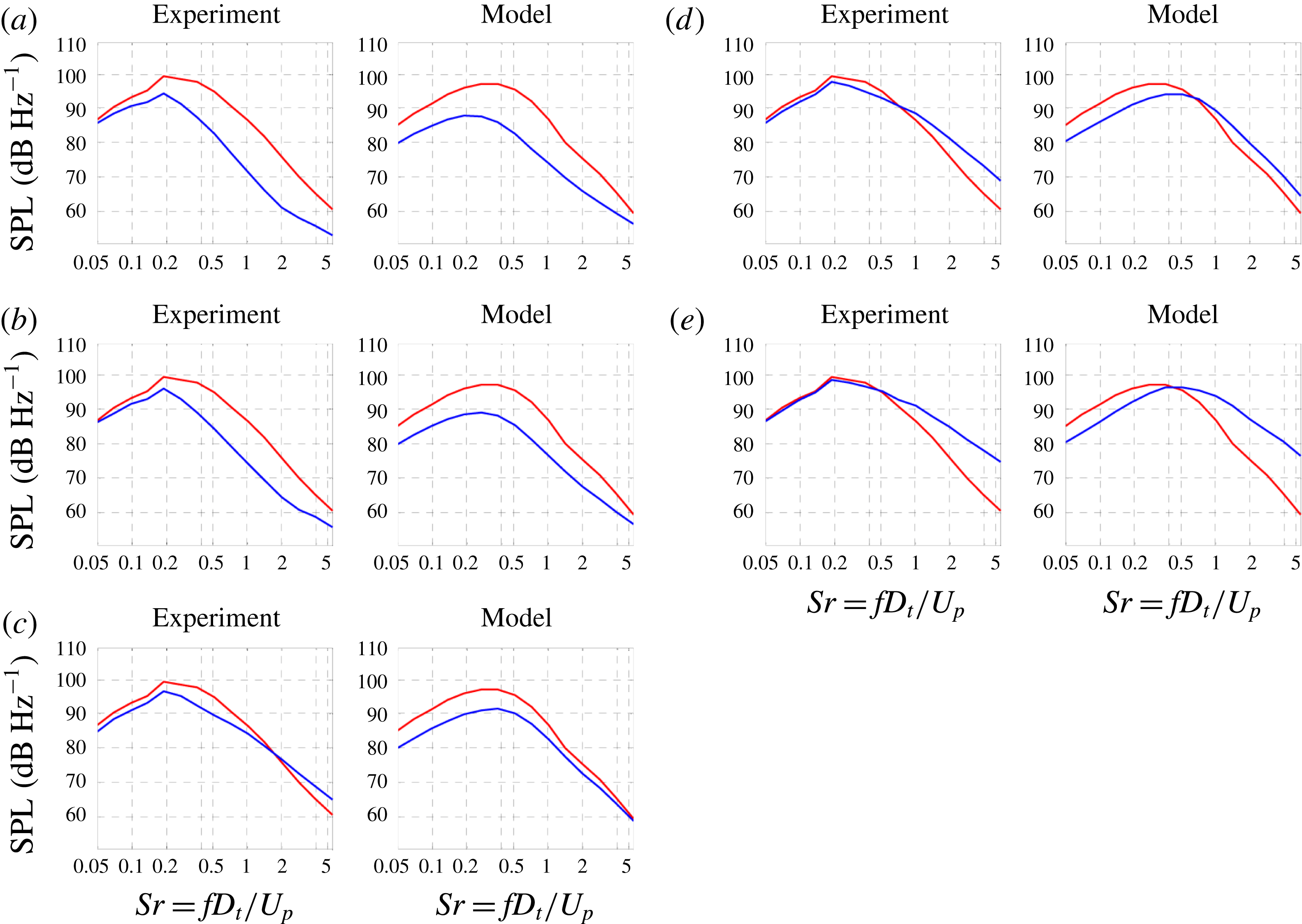
Figure 23. Experimental and modelled spectra for jets AXI04U (red) and ECC12U (blue) at polar angle
 $\unicode[STIX]{x1D703}_{0}=35^{\circ }$
. (a)
$\unicode[STIX]{x1D703}_{0}=35^{\circ }$
. (a)
 $\unicode[STIX]{x1D719}_{0}=0^{\circ }$
; (b)
$\unicode[STIX]{x1D719}_{0}=0^{\circ }$
; (b)
 $\unicode[STIX]{x1D719}_{0}=30^{\circ }$
; (c)
$\unicode[STIX]{x1D719}_{0}=30^{\circ }$
; (c)
 $\unicode[STIX]{x1D719}_{0}=60^{\circ }$
; (d)
$\unicode[STIX]{x1D719}_{0}=60^{\circ }$
; (d)
 $\unicode[STIX]{x1D719}_{0}=90^{\circ }$
; and (e)
$\unicode[STIX]{x1D719}_{0}=90^{\circ }$
; and (e)
 $\unicode[STIX]{x1D719}_{0}=180^{\circ }$
.
$\unicode[STIX]{x1D719}_{0}=180^{\circ }$
.
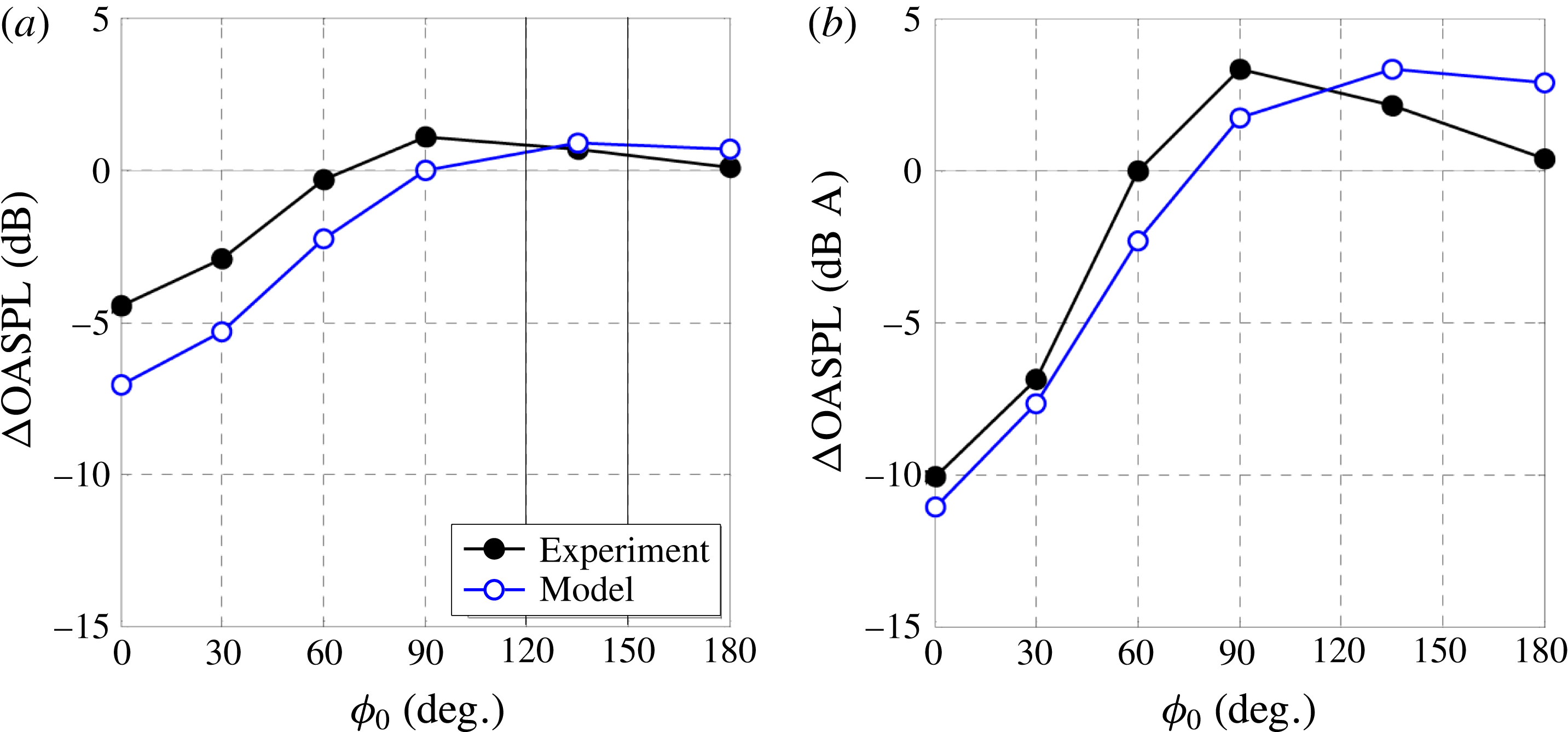
Figure 24. Experimental and modelled changes in the overall sound pressure level versus observer azimuthal angle, in the direction of peak emission, for jet ECC08U with jet AXI03U as reference. (a) No weighting; (b) A-weighting using scale factor of 40.
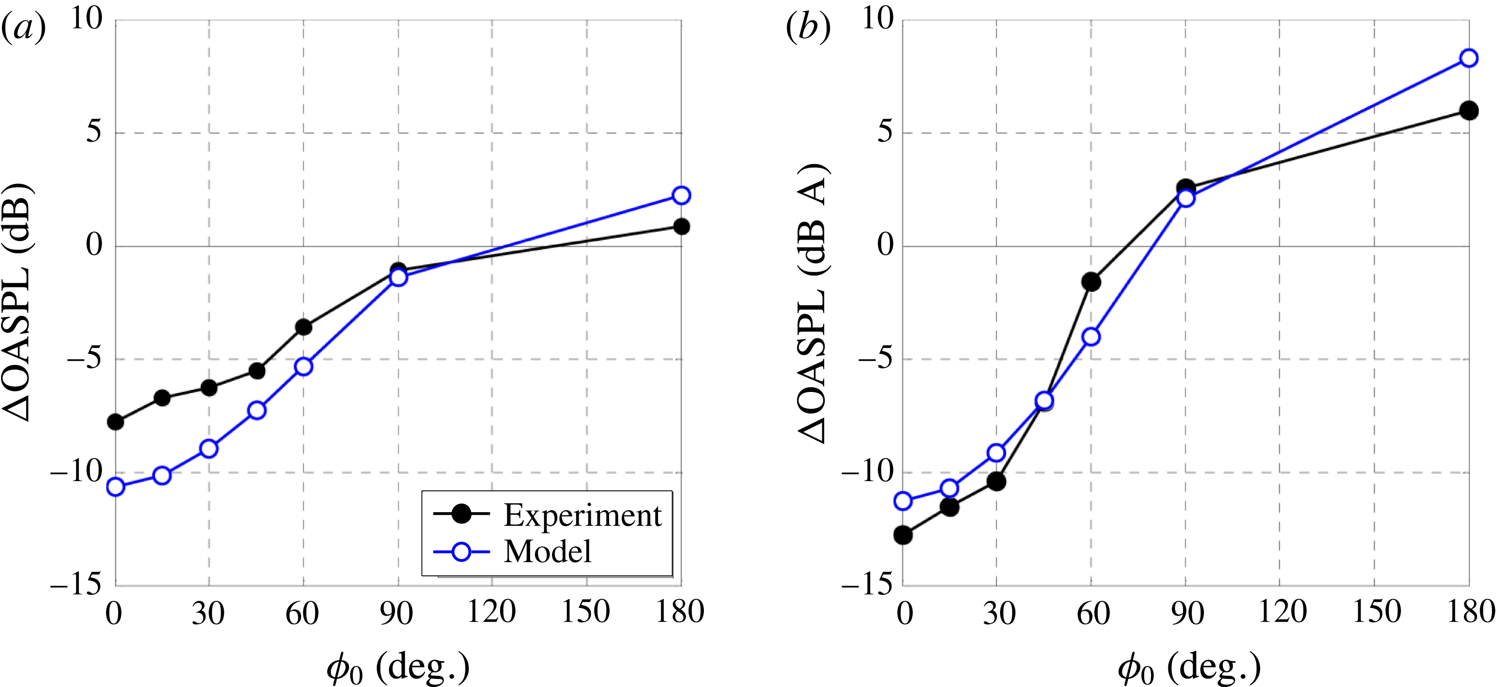
Figure 25. Experimental and modelled changes in the overall sound pressure level versus observer azimuthal angle, in the direction of peak emission, for jet ECC12U with jet AXI04U as reference. (a) No weighting; (b) A-weighting using scale factor of 40.
One may inquire whether the coefficients listed in table 3 result in physically meaningful correlation scales. Direct comparison with past acoustic analogy efforts that determined scale coefficients (e.g. Karabasov et al.
Reference Karabasov, Afsar, Hynes, Dowling, McMullan, Pokora, Page and McGuirk2010) is not feasible because of the different methodology employed here. Similarly, experimental measurements of space–time correlations are largely confined to single-stream jets at moderate velocities. Nevertheless, a broad comparison with single-stream experiments is attempted here, using
 $U$
and
$U$
and
 $D$
as the single-stream jet velocity and diameter, respectively. There is general agreement among several measurements of second-order space–time correlations (Harper-Bourne Reference Harper-Bourne2003; Bridges Reference Bridges2006; Fleury et al.
Reference Fleury, Bailly, Jondeau, Michard and Juvé2008; Kerhervé, Fitzpatrick & Kennedy Reference Kerhervé, Fitzpatrick and Kennedy2010; Morris & Zaman Reference Morris and Zaman2010b
) that, near the end of the potential core and at the lipline (which is expected to be reasonably close to the OSPS), the width the spatial decorrelation envelope (
$D$
as the single-stream jet velocity and diameter, respectively. There is general agreement among several measurements of second-order space–time correlations (Harper-Bourne Reference Harper-Bourne2003; Bridges Reference Bridges2006; Fleury et al.
Reference Fleury, Bailly, Jondeau, Michard and Juvé2008; Kerhervé, Fitzpatrick & Kennedy Reference Kerhervé, Fitzpatrick and Kennedy2010; Morris & Zaman Reference Morris and Zaman2010b
) that, near the end of the potential core and at the lipline (which is expected to be reasonably close to the OSPS), the width the spatial decorrelation envelope (
 $R_{1}$
in figure 3) ranges from roughly from
$R_{1}$
in figure 3) ranges from roughly from
 $L_{1}/D=0.5$
for the radial velocity correlation to
$L_{1}/D=0.5$
for the radial velocity correlation to
 $L_{1}/D=2.0$
for the axial velocity correlation. The corresponding width of the autocorrelation
$L_{1}/D=2.0$
for the axial velocity correlation. The corresponding width of the autocorrelation
 $\unicode[STIX]{x1D70F}_{\ast }U/D$
ranges from 0.2 for the radial velocity correlation to 0.8 for the axial velocity correlation. To compare with the present model, we plot in figure 26 the axial distributions of
$\unicode[STIX]{x1D70F}_{\ast }U/D$
ranges from 0.2 for the radial velocity correlation to 0.8 for the axial velocity correlation. To compare with the present model, we plot in figure 26 the axial distributions of
 $L_{1}/D_{t}$
and
$L_{1}/D_{t}$
and
 $\unicode[STIX]{x1D70F}_{\ast }U_{p}/D_{t}$
on the OSPS of jet AXI03U. Near the end of the primary potential core (
$\unicode[STIX]{x1D70F}_{\ast }U_{p}/D_{t}$
on the OSPS of jet AXI03U. Near the end of the primary potential core (
 $x/D_{t}=5.0$
),
$x/D_{t}=5.0$
),
 $L_{1}/D_{t}=1.50$
and
$L_{1}/D_{t}=1.50$
and
 $\unicode[STIX]{x1D70F}_{\ast }U_{p}/D_{t}=0.55$
. These values are thus consistent, in an overall sense, with the values measured in single-stream jets. The break in the distribution of
$\unicode[STIX]{x1D70F}_{\ast }U_{p}/D_{t}=0.55$
. These values are thus consistent, in an overall sense, with the values measured in single-stream jets. The break in the distribution of
 $L_{1}/D_{t}$
near
$L_{1}/D_{t}$
near
 $x/D_{t}=2$
is due to the shift of the OSPS from the outer shear layer to the inner shear layer. Assessment of the correlation scale
$x/D_{t}=2$
is due to the shift of the OSPS from the outer shear layer to the inner shear layer. Assessment of the correlation scale
 $L_{23}$
is not straightforward because it is based on the transverse projected distance
$L_{23}$
is not straightforward because it is based on the transverse projected distance
 $s$
(figure 5), for which correlation measurements do not exist, and is subject to the constraints mentioned in § 3.5.4. Similar trends are observed for jet AXI04U.
$s$
(figure 5), for which correlation measurements do not exist, and is subject to the constraints mentioned in § 3.5.4. Similar trends are observed for jet AXI04U.
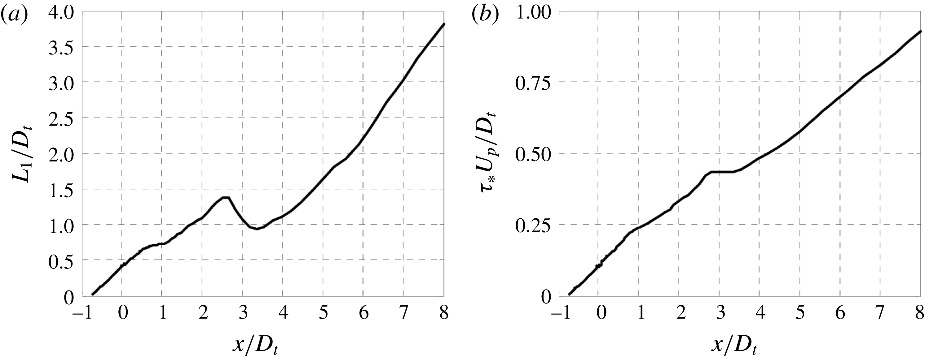
Figure 26. Axial development of correlation length scale
 $L_{1}$
and correlation time scale
$L_{1}$
and correlation time scale
 $\unicode[STIX]{x1D70F}_{\ast }$
on the OSPS of jet AXI03U.
$\unicode[STIX]{x1D70F}_{\ast }$
on the OSPS of jet AXI03U.
7 Noise reduction mechanisms
The compact expression for the spectral density (3.25) provides guidance for fundamental ways to reduce noise within a fairly constant source volume. The first approach is reduction of turbulence intensity. This influences directly the amplitude term
 $A_{0000}$
, which is linear in turbulent kinetic energy
$A_{0000}$
, which is linear in turbulent kinetic energy
 $k$
and Reynolds stress
$k$
and Reynolds stress
 $g$
. Reduction of the turbulence level by 50 %, typical of the reductions seen in figures 14 and 15, is expected to reduce noise by about 3 dB, a relatively modest amount. Thus, reduction in turbulence intensity does not explain the large spectral reductions measured in the downward direction of peak emission (figure 12).
$g$
. Reduction of the turbulence level by 50 %, typical of the reductions seen in figures 14 and 15, is expected to reduce noise by about 3 dB, a relatively modest amount. Thus, reduction in turbulence intensity does not explain the large spectral reductions measured in the downward direction of peak emission (figure 12).
The second mechanism is reduction in correlation length and time scales, manifested by the product
 $L_{1}L_{23}^{2}\unicode[STIX]{x1D70F}_{\ast }$
. In theory, this can be an effective noise suppression mechanism: if all these scales were reduced say by factor of two, the four-dimensional correlation volume would be reduced by factor of 16, translating into a 12 dB noise reduction. Breakup of eddies could be achieved with nozzle devices like chevrons, microjets, or plasma actuators (see Introduction). For practical implementation, the flow perturbations induced by such approaches would have to be small to preserve aerodynamic efficiency or minimize their energy cost. While it is possible to disorganize the turbulence in the vicinity of the nozzle, the extent to which structures at large distances from the nozzle can be affected is not clear, given the natural tendency of the shear layer to self-organize into large vortical motions (Fiedler Reference Fiedler1988).
$L_{1}L_{23}^{2}\unicode[STIX]{x1D70F}_{\ast }$
. In theory, this can be an effective noise suppression mechanism: if all these scales were reduced say by factor of two, the four-dimensional correlation volume would be reduced by factor of 16, translating into a 12 dB noise reduction. Breakup of eddies could be achieved with nozzle devices like chevrons, microjets, or plasma actuators (see Introduction). For practical implementation, the flow perturbations induced by such approaches would have to be small to preserve aerodynamic efficiency or minimize their energy cost. While it is possible to disorganize the turbulence in the vicinity of the nozzle, the extent to which structures at large distances from the nozzle can be affected is not clear, given the natural tendency of the shear layer to self-organize into large vortical motions (Fiedler Reference Fiedler1988).
The third mechanism is reduction in radiation efficiency described by the
 $\widehat{R}_{1}$
term; see also the discussion of § 3.7. To illustrate the potential of this approach, assume an exponential form for the correlation
$\widehat{R}_{1}$
term; see also the discussion of § 3.7. To illustrate the potential of this approach, assume an exponential form for the correlation
 $R_{1}(t)=\exp (-|t|)$
, so its Fourier transform is
$R_{1}(t)=\exp (-|t|)$
, so its Fourier transform is
 $\widehat{R}_{1}(\unicode[STIX]{x1D702})=2/(1+\unicode[STIX]{x1D702}^{2})$
. Then,
$\widehat{R}_{1}(\unicode[STIX]{x1D702})=2/(1+\unicode[STIX]{x1D702}^{2})$
. Then,
 $$\begin{eqnarray}\widehat{R}_{1}\left[\unicode[STIX]{x1D6FC}L_{1}\left(\frac{1}{M_{c}}-\cos \unicode[STIX]{x1D703}_{0}\right)\right]={\displaystyle \frac{2}{1+(\unicode[STIX]{x1D6FC}L_{1})^{2}\displaystyle \left(\frac{1}{M_{c}}-\cos \unicode[STIX]{x1D703}_{0}\right)^{2}}}.\end{eqnarray}$$
For Strouhal number of the order of 1, the RANS results indicate that
 $\unicode[STIX]{x1D6FC}L_{1}\sim 10$
in the most energetic regions of the flow. Now consider a reduction in
$\unicode[STIX]{x1D6FC}L_{1}\sim 10$
in the most energetic regions of the flow. Now consider a reduction in
 $M_{c}$
from 1.2 to 0.8, which is representative of the reduction noted in figure 19 for jet ECC08U near
$M_{c}$
from 1.2 to 0.8, which is representative of the reduction noted in figure 19 for jet ECC08U near
 $x/D_{t}=6$
. For
$x/D_{t}=6$
. For
 $M_{c}=1.2$
, the argument of
$M_{c}=1.2$
, the argument of
 $\widehat{R}_{1}$
is zero in the direction
$\widehat{R}_{1}$
is zero in the direction
 $\unicode[STIX]{x1D703}=35^{\circ }$
, therefore
$\unicode[STIX]{x1D703}=35^{\circ }$
, therefore
 $\widehat{R}_{1}=2$
and peak radiation efficiency is achieved (Mach wave emission). Maintaining the same angle, and reducing
$\widehat{R}_{1}=2$
and peak radiation efficiency is achieved (Mach wave emission). Maintaining the same angle, and reducing
 $M_{c}$
to 0.8 we obtain
$M_{c}$
to 0.8 we obtain
 $\widehat{R}_{1}=0.1$
, thus resulting in a 20-fold decline of the radiation efficiency term. This is consistent with large spectral declines measured in this study.
$\widehat{R}_{1}=0.1$
, thus resulting in a 20-fold decline of the radiation efficiency term. This is consistent with large spectral declines measured in this study.
It is of course difficult to completely isolate these mechanisms in an experimental or computational study. However, a rough assessment of the effect of the radiation efficiency can be obtained by setting
 $M_{c}=\overline{u}/a_{\infty }$
in the radiation efficiency term
$M_{c}=\overline{u}/a_{\infty }$
in the radiation efficiency term
 $\widehat{R}_{1}$
, instead of using (3.47). This setting, which is typically used for noise predictions in the 90 degree direction (Morris & Farassat Reference Morris and Farassat2002), does not consider the organized structure of turbulence. Therefore, the reduction in
$\widehat{R}_{1}$
, instead of using (3.47). This setting, which is typically used for noise predictions in the 90 degree direction (Morris & Farassat Reference Morris and Farassat2002), does not consider the organized structure of turbulence. Therefore, the reduction in
 $M_{c}$
noted in figures 17–20 is essentially lost. Figure 27 plots spectral comparisons analogous to those of figure 22(a) with the setting
$M_{c}$
noted in figures 17–20 is essentially lost. Figure 27 plots spectral comparisons analogous to those of figure 22(a) with the setting
 $M_{c}=\overline{u}/a_{\infty }$
. In figure 27(a), the same parameter vector (table 3, jet AXI03U) is used as with the previous approach, so naturally the baseline spectra are not matched. In figure 27(b), the parameter vector
$M_{c}=\overline{u}/a_{\infty }$
. In figure 27(a), the same parameter vector (table 3, jet AXI03U) is used as with the previous approach, so naturally the baseline spectra are not matched. In figure 27(b), the parameter vector
 $\boldsymbol{V}=[5.00,3.85,0.53,1.36,2.00]$
gives the best match between modelled and experimental spectra, although the match is much worse than that obtained with the previous
$\boldsymbol{V}=[5.00,3.85,0.53,1.36,2.00]$
gives the best match between modelled and experimental spectra, although the match is much worse than that obtained with the previous
 $M_{c}$
model. In both cases, the model fails to predict noise reduction for Strouhal numbers greater than 1, whereas in the previous approach the reductions were 10–15 dB, matching the experimental measurements (figure 22
a). These results underscore the importance of proper modelling of the radiation efficiency term and the large impact that this term has on noise prediction and noise reduction in high-speed jets.
$M_{c}$
model. In both cases, the model fails to predict noise reduction for Strouhal numbers greater than 1, whereas in the previous approach the reductions were 10–15 dB, matching the experimental measurements (figure 22
a). These results underscore the importance of proper modelling of the radiation efficiency term and the large impact that this term has on noise prediction and noise reduction in high-speed jets.
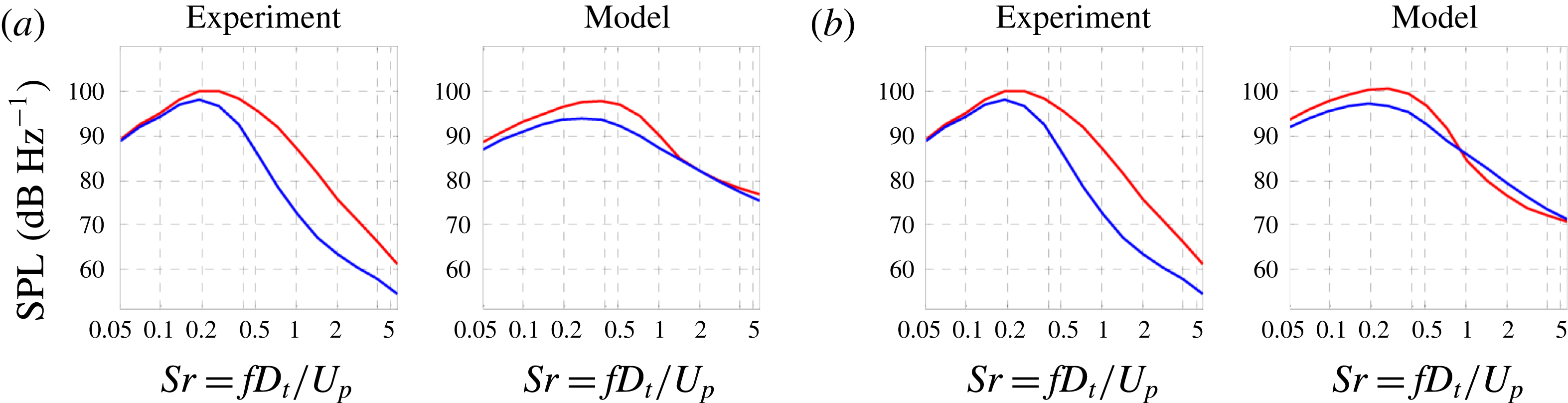
Figure 27. Assessment of model with
 $M_{c}=\overline{u}/a_{\infty }$
instead of (3.47). Experimental and modelled spectra for jets AXI03U (red) and ECC08U (blue) at
$M_{c}=\overline{u}/a_{\infty }$
instead of (3.47). Experimental and modelled spectra for jets AXI03U (red) and ECC08U (blue) at
 $\unicode[STIX]{x1D703}_{0}=35^{\circ }$
and
$\unicode[STIX]{x1D703}_{0}=35^{\circ }$
and
 $\unicode[STIX]{x1D719}_{0}=0^{\circ }$
. (a) Original parameter vector given in table 3; (b) parameter vector that minimizes difference between baseline (AXI03U) experimental and modelled spectra. Compare to figure 22(a).
$\unicode[STIX]{x1D719}_{0}=0^{\circ }$
. (a) Original parameter vector given in table 3; (b) parameter vector that minimizes difference between baseline (AXI03U) experimental and modelled spectra. Compare to figure 22(a).
8 Concluding remarks
This study was motivated by the need for a physics-based, low-order model to predict the noise changes in complex, multistream jets when the geometry of the nozzle is altered. Particular emphasis is placed on asymmetric arrangements that cause directional noise suppression. A RANS-based acoustic analogy framework was developed that addresses the noise in the polar direction of peak emission and uses the Reynolds stress as a time-averaged representation of the action of the coherent turbulent structures. The framework preserves the simplicity of the original acoustic analogy formulation by Lighthill, using the free-space Green’s function, while accounting for azimuthal effects via special forms for the space–time correlation combined with source–observer relations based on the Reynolds stress distribution in the jet plume. Below we summarize the main features of this framework and comment on its application.
A central premise in the model is that the sound emission is strongly influenced by the dynamics of the outer shear layer of the multistream jet. In a time-averaged sense, we place attention on the outermost peak of the Reynolds stress, resulting in the definition of the outer surface of peak Reynolds stress (OSPS). The mean axial velocity on this surface is thought to best represent the convective velocity of the eddies primarily responsible for peak noise emission. The axial convective Mach number, which controls the radiation efficiency, is defined accordingly. The resulting OSPS surface and convective Mach number distribution on this surfaces provide strong clues as to the noise reduction potential of a particular nozzle configuration.
To model the azimuthal effects, it was necessary to utilize a polar coordinate system centred around a properly redefined jet axis (figure 2). The new jet axis passes through the minimum value of the magnitude of the Reynolds stress inside the jet plume, and is computed practically as the centroid of the high-speed region of the jet. The use of the polar coordinate system imposes certain constraints on the types of correlations that can be used on the cross-stream plane. Source separations cannot be described in separable coordinates, necessitating the use of a mixed radial–azimuthal correlation. The usual four-dimensional Fourier transform, that gives the wavenumber–frequency spectrum in conventional formulations, is no longer possible or physical. Instead, a Hankel transform on the cross-stream plane is used in conjunction with Fourier transforms in the timewise and axial dimensions.
Modelling of the space–time correlation of the Lighthill stress tensor is the most critical step in any acoustic analogy effort. Here the space–time correlation is defined in a fixed frame of reference. Its axial–timewise formulation is designed to reproduce qualitatively the main features of the axial space–time correlation measured by a large number of past works, and uses the aforementioned definition of axial convective velocity. The cross-stream correlation is based on the projected distance between two source elements, a formulation that helps ensure that the modelled power spectral density is real and non-negative. An important feature is the inclusion of a transverse space–time correlation and associated transverse convective velocity. In conjunction with the Hankel transform, the transverse propagation induces an azimuthal directivity in the far-field spectral density. The axial and timewise correlation functions are modelled as stretched exponentials, enabling a flexibility that is very significant for calibrating the model. The cross-stream correlation is limited to a Gaussian form for numerical efficiency.
The acoustic analogy model is calibrated based on knowledge of the spectral density of a reference (axisymmetric) jet. In the present study, a five-element parameter vector controls the characteristic scales and shape coefficients of the correlation functions. The vector is determined via conjugate-gradient minimization of a cost function comprising the difference between the modelled and experimental spectra of the reference jet as well as penalty functions that constrain the parameters. This parameter vector is then applied to the non-reference jets.
Results were presented for two sets of triple-stream jets, each set comprising a coaxial reference jet and at least one asymmetric variant. A total of three asymmetric jets were covered in this study, two featuring eccentric tertiary ducts and one combining eccentric secondary and tertiary ducts. There is an excellent match between the experimental and modelled reference jets. The model captures the azimuthal noise trends of the asymmetric jets, and reproduces reasonably well the measured noise reduction. The azimuthal variation of the A-weighted OASPL, in particular, is reproduced with an accuracy of about 1 dB. A preliminary evaluation of the noise suppression mechanisms indicates that the noise reduction of the asymmetric jets is caused primarily by the reduction in radiation efficiency.
Regarding the numerical efficiency of the acoustic analogy scheme, once the RANS solutions are available for the reference and non-reference jets, the prediction of their spectral densities consumes on the order of one hour on a basic personal computer. This includes the parameterization process of § 4, in conjunction with the methods described in appendix A.
Acknowledgements
The support by NASA Cooperative Agreement NNX14AR98A, monitored Dr J. Bridges, is gratefully acknowledged. The author thanks Dr V. Phong and Dr J. Xiong for their contributions in the experiments and computations, respectively.
Appendix A
Efficient computation of the power spectral density is important for the development of practical predictive tools. Efficiency is particularly desirable for the baseline, axisymmetric jets that will be subject to optimization routines requiring computation of the power spectral density a large number of times.
A.1 General relations
Combining (3.25) and (3.45), we express the spectral density as the following set of equations:
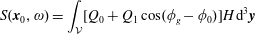 $$\begin{eqnarray}\displaystyle & \displaystyle S(\boldsymbol{x}_{0},\unicode[STIX]{x1D714})=\int _{{\mathcal{V}}}[Q_{0}+Q_{1}\cos (\unicode[STIX]{x1D719}_{g}-\unicode[STIX]{x1D719}_{0})]H\,\text{d}^{3}\boldsymbol{y} & \displaystyle\end{eqnarray}$$
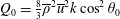 $$\begin{eqnarray}\displaystyle & \displaystyle Q_{0}={\textstyle \frac{8}{3}}\overline{\unicode[STIX]{x1D70C}}^{2}\overline{u}^{2}k\cos ^{2}\unicode[STIX]{x1D703}_{0} & \displaystyle\end{eqnarray}$$
 $$\begin{eqnarray}\displaystyle & \displaystyle Q_{1}=8\overline{\unicode[STIX]{x1D70C}}^{2}\overline{u}^{2}g\cos ^{3}\unicode[STIX]{x1D703}_{0}\sin \unicode[STIX]{x1D703}_{0} & \displaystyle\end{eqnarray}$$
 $$\begin{eqnarray}\displaystyle & \displaystyle H=\frac{\unicode[STIX]{x1D6FC}^{4}}{16\unicode[STIX]{x03C0}{\mathcal{R}}^{2}}\unicode[STIX]{x1D70F}_{\ast }L_{1}\unicode[STIX]{x03C0}L_{23}^{2}\widehat{R}_{1}\widehat{R}_{4}\widetilde{R}_{23}. & \displaystyle\end{eqnarray}$$
A.2 Treatment of half-jet
Time-averaged computations of jet flows having a plane of symmetry typically treat only one half of the jet. In these cases, it is important to be able to compute the power spectral density based on the half-jet data, that is, without creating the mirror image and thus doubling the computational cost. Even for computations that treat the entire jet, the ability to compute the power spectral density using only the symmetric half of the data provides important computational savings.
Focusing on the azimuthal component of the integration of (A 1), and showing only the azimuthal dependence of the variables involved, we examine the treatment of the integral
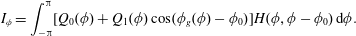 $$\begin{eqnarray}I_{\unicode[STIX]{x1D719}}=\int _{-\unicode[STIX]{x03C0}}^{\unicode[STIX]{x03C0}}[Q_{0}(\unicode[STIX]{x1D719})+Q_{1}(\unicode[STIX]{x1D719})\cos (\unicode[STIX]{x1D719}_{g}(\unicode[STIX]{x1D719})-\unicode[STIX]{x1D719}_{0})]H(\unicode[STIX]{x1D719},\unicode[STIX]{x1D719}-\unicode[STIX]{x1D719}_{0})\,\text{d}\unicode[STIX]{x1D719}.\end{eqnarray}$$
For the source term
 $H$
, the notation
$H$
, the notation
 $H(\unicode[STIX]{x1D719},\unicode[STIX]{x1D719}-\unicode[STIX]{x1D719}_{0})$
indicates the azimuthal dependence of the scales as well as the azimuthal directivity of
$H(\unicode[STIX]{x1D719},\unicode[STIX]{x1D719}-\unicode[STIX]{x1D719}_{0})$
indicates the azimuthal dependence of the scales as well as the azimuthal directivity of
 $\widetilde{R}_{23}$
that involves the term
$\widetilde{R}_{23}$
that involves the term
 $\cos (\unicode[STIX]{x1D719}-\unicode[STIX]{x1D719}_{0})$
in (3.33). We note the following dependencies across the symmetry plane:
$\cos (\unicode[STIX]{x1D719}-\unicode[STIX]{x1D719}_{0})$
in (3.33). We note the following dependencies across the symmetry plane:
 $$\begin{eqnarray}\left.\begin{array}{@{}c@{}}\displaystyle Q_{0}(-\unicode[STIX]{x1D719})=Q_{0}(\unicode[STIX]{x1D719})\\ \displaystyle Q_{1}(-\unicode[STIX]{x1D719})=Q_{1}(\unicode[STIX]{x1D719})\\ \displaystyle \unicode[STIX]{x1D719}_{g}(-\unicode[STIX]{x1D719})=-\unicode[STIX]{x1D719}_{g}(\unicode[STIX]{x1D719})\\ \displaystyle H(-\unicode[STIX]{x1D719},-\unicode[STIX]{x1D719}-\unicode[STIX]{x1D719}_{0})=H(\unicode[STIX]{x1D719},\unicode[STIX]{x1D719}+\unicode[STIX]{x1D719}_{0}).\end{array}\right\}\end{eqnarray}$$
It is now easy to show that the full-circle integral of (A 2) is equivalent to the integral over the half-circle
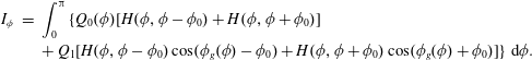 $$\begin{eqnarray}\displaystyle I_{\unicode[STIX]{x1D719}} & = & \displaystyle \int _{0}^{\unicode[STIX]{x03C0}}\{\!Q_{0}(\unicode[STIX]{x1D719})[H(\unicode[STIX]{x1D719},\unicode[STIX]{x1D719}-\unicode[STIX]{x1D719}_{0})+H(\unicode[STIX]{x1D719},\unicode[STIX]{x1D719}+\unicode[STIX]{x1D719}_{0})]\nonumber\\ \displaystyle & & \displaystyle +\,Q_{1}[H(\unicode[STIX]{x1D719},\unicode[STIX]{x1D719}-\unicode[STIX]{x1D719}_{0})\cos (\unicode[STIX]{x1D719}_{g}(\unicode[STIX]{x1D719})-\unicode[STIX]{x1D719}_{0})+H(\unicode[STIX]{x1D719},\unicode[STIX]{x1D719}+\unicode[STIX]{x1D719}_{0})\cos (\unicode[STIX]{x1D719}_{g}(\unicode[STIX]{x1D719})+\unicode[STIX]{x1D719}_{0})]\!\}\,\text{d}\unicode[STIX]{x1D719}.\nonumber\\ \displaystyle & & \displaystyle\end{eqnarray}$$
This procedure allows the evaluation of the power spectral density by integration over the volume of the half-jet.
A.3 Special treatment for axisymmetric jets
For axisymmetric jets, the computational cost can be further reduced by confining the volume integral to an azimuthal slice of the jet. This is not a simple reduction because it needs to account for the source–observer azimuthal dependencies in
 $A_{0000}$
(i.e. the cosine terms in (A 1)) as well as the azimuthal influence contained in
$A_{0000}$
(i.e. the cosine terms in (A 1)) as well as the azimuthal influence contained in
 $\widetilde{R}_{23}$
. Having an analytical relation for
$\widetilde{R}_{23}$
. Having an analytical relation for
 $\widetilde{R}_{23}$
is very useful in this regard. Using (3.33), the source term
$\widetilde{R}_{23}$
is very useful in this regard. Using (3.33), the source term
 $H$
of (A 1d
) is expressed as
$H$
of (A 1d
) is expressed as
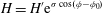 $$\begin{eqnarray}\displaystyle & \displaystyle H=H^{\prime }\text{e}^{\unicode[STIX]{x1D70E}\cos (\unicode[STIX]{x1D719}-\unicode[STIX]{x1D719}_{0})} & \displaystyle\end{eqnarray}$$
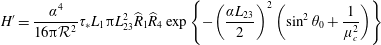 $$\begin{eqnarray}\displaystyle & \displaystyle H^{\prime }=\frac{\unicode[STIX]{x1D6FC}^{4}}{16\unicode[STIX]{x03C0}{\mathcal{R}}^{2}}\unicode[STIX]{x1D70F}_{\ast }L_{1}\unicode[STIX]{x03C0}L_{23}^{2}\widehat{R}_{1}\widehat{R}_{4}\exp \left\{-\!\left(\frac{\unicode[STIX]{x1D6FC}L_{23}}{2}\right)^{2}\left(\sin ^{2}\unicode[STIX]{x1D703}_{0}+\frac{1}{\unicode[STIX]{x1D707}_{c}^{2}}\right)\right\} & \displaystyle\end{eqnarray}$$
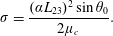 $$\begin{eqnarray}\displaystyle & \displaystyle \unicode[STIX]{x1D70E}=\frac{(\unicode[STIX]{x1D6FC}L_{23})^{2}\sin \unicode[STIX]{x1D703}_{0}}{2\unicode[STIX]{x1D707}_{c}}. & \displaystyle\end{eqnarray}$$
 $\unicode[STIX]{x1D719}_{g}$
equals the geometric azimuthal angle
$\unicode[STIX]{x1D719}_{g}$
equals the geometric azimuthal angle
 $\unicode[STIX]{x1D719}$
. This is valid for a mean velocity profile that is monotonically decreasing with radius and is applicable to the dominant source region of the axisymmetric jets under consideration here. Then (A 1a
) becomes
$\unicode[STIX]{x1D719}$
. This is valid for a mean velocity profile that is monotonically decreasing with radius and is applicable to the dominant source region of the axisymmetric jets under consideration here. Then (A 1a
) becomes 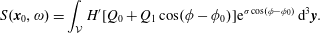 $$\begin{eqnarray}S(\boldsymbol{x}_{0},\unicode[STIX]{x1D714})=\int _{{\mathcal{V}}}H^{\prime }[Q_{0}+Q_{1}\cos (\unicode[STIX]{x1D719}-\unicode[STIX]{x1D719}_{0})]\text{e}^{\unicode[STIX]{x1D70E}\cos (\unicode[STIX]{x1D719}-\unicode[STIX]{x1D719}_{0})}\,\text{d}^{3}\boldsymbol{y}.\end{eqnarray}$$
Noting that
 $H^{\prime }$
,
$H^{\prime }$
,
 $Q_{0}$
and
$Q_{0}$
and
 $Q_{1}$
are all purely axisymmetric, the only azimuthal dependence in the integrand comes from the
$Q_{1}$
are all purely axisymmetric, the only azimuthal dependence in the integrand comes from the
 $\cos (\unicode[STIX]{x1D719}-\unicode[STIX]{x1D719}_{0})$
terms. Invoking the integral representations of the modified Bessel functions, the azimuthal component of the integration results in the terms
$\cos (\unicode[STIX]{x1D719}-\unicode[STIX]{x1D719}_{0})$
terms. Invoking the integral representations of the modified Bessel functions, the azimuthal component of the integration results in the terms
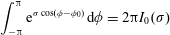 $$\begin{eqnarray}\displaystyle & \displaystyle \int _{-\unicode[STIX]{x03C0}}^{\unicode[STIX]{x03C0}}\text{e}^{\unicode[STIX]{x1D70E}\cos (\unicode[STIX]{x1D719}-\unicode[STIX]{x1D719}_{0})}\,\text{d}\unicode[STIX]{x1D719}=2\unicode[STIX]{x03C0}I_{0}(\unicode[STIX]{x1D70E}) & \displaystyle\end{eqnarray}$$
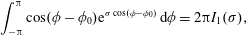 $$\begin{eqnarray}\displaystyle & \displaystyle \int _{-\unicode[STIX]{x03C0}}^{\unicode[STIX]{x03C0}}\cos (\unicode[STIX]{x1D719}-\unicode[STIX]{x1D719}_{0})\text{e}^{\unicode[STIX]{x1D70E}\cos (\unicode[STIX]{x1D719}-\unicode[STIX]{x1D719}_{0})}\,\text{d}\unicode[STIX]{x1D719}=2\unicode[STIX]{x03C0}I_{1}(\unicode[STIX]{x1D70E}), & \displaystyle\end{eqnarray}$$
where
 $I_{0}$
and
$I_{0}$
and
 $I_{1}$
are the modified Bessel functions of the first kind and of orders zero and one, respectively. Now (A 6) collapses into the two-dimensional integral
$I_{1}$
are the modified Bessel functions of the first kind and of orders zero and one, respectively. Now (A 6) collapses into the two-dimensional integral
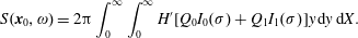 $$\begin{eqnarray}S(\boldsymbol{x}_{0},\unicode[STIX]{x1D714})=2\unicode[STIX]{x03C0}\int _{0}^{\infty }\int _{0}^{\infty }H^{\prime }[Q_{0}I_{0}(\unicode[STIX]{x1D70E})+Q_{1}I_{1}(\unicode[STIX]{x1D70E})]y\,\text{d}y\,\text{d}X.\end{eqnarray}$$
While in theory the reduction to two dimensions cuts down the computational demands dramatically, the expectation of sufficiently resolved data on a given meridional section is not realistic. Computational codes produce data in three-dimensional grids that may not be purely axisymmetric (even for the treatment of axisymmetric jets) and thus cannot be readily transformed into a radial set. Interpolation on a meridional section presents numerical challenges that can introduce errors with large impact on the noise prediction, particularly in the very thin shear layers near the nozzle exit. On the other hand, restricting the integration to an azimuthal slice containing a sufficient population of elements is a very simple procedure. It is accomplished here by realizing that (A 9) is equivalent to
 $$\begin{eqnarray}S(\boldsymbol{x}_{0},\unicode[STIX]{x1D714})=\frac{2\unicode[STIX]{x03C0}}{\unicode[STIX]{x1D6F7}}\int _{0}^{\unicode[STIX]{x1D6F7}}\int _{0}^{\infty }\int _{0}^{\infty }H^{\prime }[Q_{0}I_{0}(\unicode[STIX]{x1D70E})+Q_{1}I_{1}(\unicode[STIX]{x1D70E})]y\,\text{d}y\,\text{d}X\,\text{d}\unicode[STIX]{x1D719}.\end{eqnarray}$$
The integral now represents a volumetric integration over an azimuthal slice of angle
 $\unicode[STIX]{x1D6F7}$
, and can be expressed compactly as
$\unicode[STIX]{x1D6F7}$
, and can be expressed compactly as
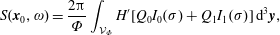 $$\begin{eqnarray}S(\boldsymbol{x}_{0},\unicode[STIX]{x1D714})=\frac{2\unicode[STIX]{x03C0}}{\unicode[STIX]{x1D6F7}}\int _{{\mathcal{V}}_{\unicode[STIX]{x1D6F7}}}H^{\prime }[Q_{0}I_{0}(\unicode[STIX]{x1D70E})+Q_{1}I_{1}(\unicode[STIX]{x1D70E})]\,\text{d}^{3}\boldsymbol{y},\end{eqnarray}$$
where
 ${\mathcal{V}}_{\unicode[STIX]{x1D6F7}}$
is the volume of the slice. Through experimentation it was determined that a
${\mathcal{V}}_{\unicode[STIX]{x1D6F7}}$
is the volume of the slice. Through experimentation it was determined that a
 $5^{\circ }$
azimuthal slice contained a sufficient number of elements to compute the power spectral density with excellent accuracy, within a few tenths of a decibel, as compared to integration over the entire volume. The resulting 36-fold reduction in computational time, relative to treating the entire half-jet, benefits tremendously the conjugate-gradient minimization process described in § 4.2, which requires evaluation of the spectral density of the order of 100 times.
$5^{\circ }$
azimuthal slice contained a sufficient number of elements to compute the power spectral density with excellent accuracy, within a few tenths of a decibel, as compared to integration over the entire volume. The resulting 36-fold reduction in computational time, relative to treating the entire half-jet, benefits tremendously the conjugate-gradient minimization process described in § 4.2, which requires evaluation of the spectral density of the order of 100 times.


