


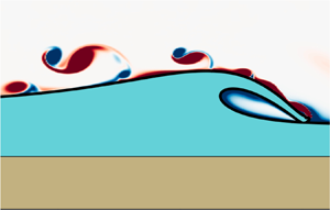



1. Introduction
As they approach shore, shoaling waves change shape, becoming steeper with narrower peaks and more pitched forward (e.g. Elgar & Guza Reference Elgar and Guza1985). Once sufficiently steepened, depth-limited wave breaking occurs with wave overturning, and subsequently the overturn jet impacts the water surface in front of the wave. Depth-limited wave breaking is often qualitatively categorized into spilling and plunging (e.g. Peregrine Reference Peregrine1983), where spilling waves have very small overturns, and plunging waves have larger overturns. Bathymetry along with offshore wave height and wavelength are well understood (e.g. via the Iribarren number) to be important in setting spilling or plunging wave breaking (e.g. Peregrine Reference Peregrine1983). For example, larger planar beach slope  $\beta$ leads to larger overturns (Grilli, Svendsen & Subramanya Reference Grilli, Svendsen and Subramanya1997; Mostert & Deike Reference Mostert and Deike2020; O'Dea, Brodie & Elgar Reference O'Dea, Brodie and Elgar2021). Across laboratory and field observations, the wave overturn shape is important in the resulting splash up and bubble entrainment (Chanson & Jaw-Fang Reference Chanson and Jaw-Fang1997; Yasuda et al. Reference Yasuda, Mutsuda, Mizutani and Matsuda1999; Blenkinsopp & Chaplin Reference Blenkinsopp and Chaplin2007), water column turbulence (Ting & Kirby Reference Ting and Kirby1995, Reference Ting and Kirby1996; Aagaard, Hughes & Ruessink Reference Aagaard, Hughes and Ruessink2018), sediment suspension (e.g. Aagaard et al. Reference Aagaard, Hughes and Ruessink2018), and wave impact forces on engineered structures (Bullock et al. Reference Bullock, Obhrai, Peregrine and Bredmose2007). Similarly in numerical simulations of deep-water and depth-limited wave breaking, the geometry of wave overturning impacts air entrainment, vorticity generation, and pathways of turbulent dissipation (e.g. Lubin et al. Reference Lubin, Vincent, Abadie and Caltagirone2006; Derakhti & Kirby Reference Derakhti and Kirby2014; Mostert, Popinet & Deike Reference Mostert, Popinet and Deike2022). Thus understanding the factors that affect the shape of overturning waves is important to a range of processes.
In deep water, wind is well understood to lead to surface gravity wave growth and decay (e.g. Miles Reference Miles1957; Phillips Reference Phillips1957). However, wind can also change wave shape in both deep (Leykin et al. Reference Leykin, Donelan, Mellen and McLaughlin1995; Zdyrski & Feddersen Reference Zdyrski and Feddersen2020) and shallow (Zdyrski & Feddersen Reference Zdyrski and Feddersen2021) water, as well as in shoaling waves (Feddersen & Veron Reference Feddersen and Veron2005; Sous et al. Reference Sous, Forsberg, Touboul and Gonçalves Nogueira2021; Zdyrski & Feddersen Reference Zdyrski and Feddersen2022). In laboratory studies, onshore wind results in wave breaking in deeper water (farther offshore) (Douglass Reference Douglass1990; Sous et al. Reference Sous, Forsberg, Touboul and Gonçalves Nogueira2021), with the opposite for offshore wind. Feddersen et al. (Reference Feddersen, Fincham, Brodie, Young, Spydell, Grimes, Pieszka and Hanson2023) studied the explicit wind dependence of overturn wave shape at the Surf Ranch, a wave basin designed for surfing. A field-scale shoaling solitary wave with height  ${\approx }2.25$ m propagated at $C=6.7\ \mathrm {m}\ \mathrm {s}^{-1}$ and overturned. The cross-wave component of wind $U$, measured 16 m above the water surface, varied from onshore to offshore with realistic $-1.2 < U/C < 0.7$. The non-dimensionalized breakpoint location was inversely related to $U/C$, consistent with Douglass (Reference Douglass1990). The non-dimensional overturn area $A/H_b^2$, where $H_b$ is breaking wave height, and overturn aspect ratio (overturn width divided by length) were also inversely related to $U/C$, with smaller area and overturns for increasing onshore wind (positive $U/C$). For increasing offshore wind, $A/H_b^2$ was approximately uniform. The non-dimensional overturn parameters varied by a factor of two for the observed $U/C$, indicating that the wind has a significant effect on overturn shape. However, the mechanism by which wind induces these geometric changes is uncertain. For example, the pressure profiles induced by the wind on the different parts of the evolving wave, along with the general flow structure over and around the wave, remain unknown.
Numerical modelling offers a promising avenue for investigating wind effects on shoaling and overturning wave shape. For over two decades, volume-of-fluid (VOF) based numerical models have enabled the study of various aspects of wave breaking (e.g. Lin & Liu Reference Lin and Liu1998; Chen et al. Reference Chen, Kharif, Zaleski and Li1999; Guignard et al. Reference Guignard, Marcer, Rey, Kharif and Fraunié2001). More recent advances in two-phase numerical modelling in both direct numerical simulations (DNS) and large-eddy simulations (LES) has enabled significant advances in understanding aspects of deep (Lubin et al. Reference Lubin, Kimmoun, Véron and Glockner2019; Mostert et al. Reference Mostert, Popinet and Deike2022) and shallow (e.g. Lubin & Glockner Reference Lubin and Glockner2015; Mostert & Deike Reference Mostert and Deike2020; Boswell, Yan & Mostert Reference Boswell, Yan and Mostert2023; Liu et al. Reference Liu, Wang, Bayeul-Lainé, Li, Katz and Coutier-Delgosha2023) water wave breaking. Similar advances have occurred in the study of wind input of energy and momentum to deep-water waves with coupled (e.g. Hao & Shen Reference Hao and Shen2019) and VOF (Wu, Popinet & Deike Reference Wu, Popinet and Deike2022) models. Numerical studies using two-dimensional (2-D) two-phase RANS solvers of wind-forced solitary (Xie Reference Xie2014) and progressive (Xie Reference Xie2017) waves have seen a wind-induced shift in breakpoint location analogous to laboratory experiments. Analogous wind effects were seen in 2-D LES of deep-water wave breaking (Chen & Zou Reference Chen and Zou2022). However, the effect of wind on shoaling and overturning waves has not been studied in detail with numerical models.
Here, we study the wind effects on solitary wave shoaling and overturning for a model domain similar to that of Feddersen et al. (Reference Feddersen, Fincham, Brodie, Young, Spydell, Grimes, Pieszka and Hanson2023) using the two-phase numerical model Basilisk run in two dimensions up until the moment when the overturning jet impacts. The breaking processes that occur after jet impact have been and are actively being studied with numerical models (e.g. Lin & Liu Reference Lin and Liu1998; Mostert & Deike Reference Mostert and Deike2020; Boswell et al. Reference Boswell, Yan and Mostert2023; Liu et al. Reference Liu, Wang, Bayeul-Lainé, Li, Katz and Coutier-Delgosha2023; Chen, Raubenheimer & Elgar Reference Chen, Raubenheimer and Elgar2024). In § 2, the model set-up is described, the key non-dimensional parameters (including wind Reynolds number  ${Re}^*$) are defined, and the relationship between modelled air velocity $\langle \bar {U} \rangle /C$ and ${Re}^*$ is discussed. In § 3.1, the qualitative features of the shoaling solitary wave and air vorticity are examined for strong onshore and offshore wind. The statistics of solitary wave shoaling under strong onshore and offshore wind are described in § 3.2. Overturn wave shape is quantified by geometrical parameters defined at the moment of jet impact (§ 3.3). The relationship of the non-dimensional geometrical parameters (defined in § 3.4) to ${Re}^*$ is examined (§ 3.5). The relative strength of viscous stresses and pressure at the air–water interface is examined in § 3.6, and the terms of the surface dynamic boundary condition, including pressure variations and surface tension, are analysed in § 3.7. We discuss the shoaling results relative to previous studies, examine potential reasons for the differences between our results here and those of field-scale experiments, and consider implications in § 4. Section 5 provides a summary.
2. Methods
We numerically simulate in two dimensions the shoaling and overturning of a solitary wave with the two-phase incompressible Navier–Stokes equations using the open-source Basilisk software package (Popinet Reference Popinet2003, Reference Popinet2009, Reference Popinet2018) for solving partial differential equations on an adaptively refined grid. Basilisk has been used extensively to model wave breaking (Deike, Popinet & Melville Reference Deike, Popinet and Melville2015; Deike, Melville & Popinet Reference Deike, Melville and Popinet2016; Mostert & Deike Reference Mostert and Deike2020; Mostert et al. Reference Mostert, Popinet and Deike2022) as well as wave interactions with wind (Wu & Deike Reference Wu and Deike2021; Wu et al. Reference Wu, Popinet and Deike2022).
2.1. Formulation and governing equations
The governing equations are the two-phase (water and air) Navier–Stokes equations in two dimensions, given as
 \begin{equation} \left.\begin{array}{c@{}} \displaystyle \dfrac{\partial \rho}{\partial t} + \boldsymbol{\nabla} \boldsymbol{\cdot} (\rho\boldsymbol{u}) = 0,\\ \displaystyle \rho\left(\dfrac{\partial \boldsymbol{u}}{\partial t} +\boldsymbol{u} \boldsymbol{\cdot} \boldsymbol{\nabla} \boldsymbol{u}\right) ={-}\boldsymbol{\nabla} p + \rho \boldsymbol{g} + \boldsymbol{\nabla} \boldsymbol{\cdot} (2\mu \boldsymbol{D}) + \sigma \kappa \boldsymbol{n}\delta_s,\\ \boldsymbol{\nabla} \boldsymbol{\cdot} \boldsymbol{u} = 0, \end{array}\right\} \end{equation}
where  $\boldsymbol {u}, \sigma, \kappa, \boldsymbol {D}, \boldsymbol {g}$ are the fluid velocity, surface tension, curvature of the interface, deformation tensor and acceleration due to gravity, respectively. In component form, the 2-D fluid velocity is $\boldsymbol {u} = (u,w)$, where $u$ and $w$ are the horizontal and vertical velocities, respectively. For each fluid, the water and air densities ( $\rho _{w},\rho _{a}$) and dynamic viscosities ( $\mu _{w},\mu _{a}$) are uniform. A VOF advection scheme with a colour function $f$ is used to capture and advect the air–water interface in a momentum-conserving implementation. Hence for two-phase mixtures, $\rho$ and $\mu$ are represented by
 \begin{equation} \left.\begin{array}{c@{}} \rho = f\rho_{w} + (1-f)\rho_{a}, \\ \mu = f\mu_{w} + (1-f)\mu_{a}, \end{array}\right\} \end{equation}
where  $f$ is interpreted as the liquid volume fraction ( $\,f=1$ for water, $f=0$ for air). The water-to-air ratios for $\rho$ and $\mu$ are important non-dimensional parameters and are here held fixed at $\rho _{a}/\rho _{w} = 0.001$ and $\mu _{a}/\mu _{w} = 0.018$. The air–water interface requires continuity of velocity and stress, including surface tension. Surface tension as the interfacial force $\sigma \kappa \boldsymbol {n}\delta _s$ is determined from the Dirac delta $\delta _s$ on the interface and the unit normal vector $\boldsymbol {n}$. This formulation is expressed in Popinet (Reference Popinet2018), alongside the implementation of gravity as an interfacial force. In (2.1), we substitute
 \begin{equation} \rho \boldsymbol{g} \to (\rho_{a} - \rho_{w}) (\boldsymbol{g}\boldsymbol{\cdot} \boldsymbol{x}) \boldsymbol{n}\delta_s, \end{equation}
which are equal, up to a difference in the pressure field. The reduced-gravity implementation avoids the appearance of spurious velocities and unphysical energy production near the air–water interface (Wroniszewski, Verschaeve & Pedersen Reference Wroniszewski, Verschaeve and Pedersen2014).
The two-phase incompressible Navier–Stokes equations are solved on an adaptive Cartesian mesh using the Bell–Colella–Glaz projection method (Bell, Colella & Glaz Reference Bell, Colella and Glaz1989) with the VOF scheme described above, allowing for a sharp interface between phases (Fuster & Popinet Reference Fuster and Popinet2018; van Hooft et al. Reference van Hooft, Popinet, van Heerwaarden, van der Linden, de Roode and van de Wiel2018; López-Herrera, Popinet & Castrejón-Pita Reference López-Herrera, Popinet and Castrejón-Pita2019). The bathymetry is represented with an additional volume fraction field as an embedded boundary (Johansen & Colella Reference Johansen and Colella1998). Surface tension is implemented using the continuum surface force approach due to Brackbill, Kothe & Zemach (Reference Brackbill, Kothe and Zemach1992).
2.1.1. Model domain and boundary conditions
The model domain (figure 1) is similar to that used in Boswell et al. (Reference Boswell, Yan and Mostert2023), with modifications to be analogous to the bathymetry of the Surf Ranch (Feddersen et al. Reference Feddersen, Fincham, Brodie, Young, Spydell, Grimes, Pieszka and Hanson2023). In the offshore region, the bathymetry is flat with depth  $h_0$, and the total cross-shore ( $x$) domain size is $L_x = 60h_0$. The offshore flat bathymetry extends for $x/h_0$ distance $30$. At $x/h_0=30$, the bathymetry slopes upwards with slope $\beta = 0.0693$ over $x/h_0$ distance $9.08$ to a shallow depth $h_s/h_0 = 0.371$, which then extends an $x/h_0$ distance of nearly $20$. The bathymetric slope is a key non-dimensional parameter well understood to affect overturn shape (e.g. Grilli et al. Reference Grilli, Svendsen and Subramanya1997; Mostert & Deike Reference Mostert and Deike2020; O'Dea et al. Reference O'Dea, Brodie and Elgar2021). Here, $\beta$ is held fixed to the Surf Ranch bathymetric slope projected in the direction of wave propagation (Feddersen et al. Reference Feddersen, Fincham, Brodie, Young, Spydell, Grimes, Pieszka and Hanson2023) in order to isolate the wind effects on overturning shape. The bathymetry has a no-slip boundary condition for fluid velocity. At the ends of the model domain at $x=0$ and $x/h_0=60$, vertical walls extend from the bathymetry to the still-water depth at $z/h_0=0$, with associated $u=0$ and no-slip boundary conditions. The air domain extends vertically from the water surface (mostly near $z/h_0 = 0$) to $z/h_0 = h_a/h_0 = 10$, where a ‘ceiling’, with a free-slip boundary condition, is placed on the domain (figure 1). In the range $0 < z/h_0 < 10$, at the left and right boundaries ( $x/h_0=0$ and $x/h_0=60$, figure 1), open boundaries allow for air flow in and out of the domain. The inlet and outlet locations vary depending on the wind direction. For onshore winds, the left side is the inlet, and for offshore winds, the right side is the inlet. A Neumann condition is placed on the dynamic pressure, $\partial p/\partial x=0$, on the inlet, and a Dirichlet dynamic pressure condition $p=0$ is placed on the outlet, both uniformly in the vertical.

Figure 1. The simulation domain just after initialization as a function of non-dimensional horizontal  $x/h_0$ and vertical $z/h_0$ coordinates. The brown region represents the bathymetry, the aqua blue is water, the air–sea interface is indicated by the black curve, and air vorticity is given by the colour bar. The deeper flat water at $x/h_0 < 30$ has depth $h_0$ such that the bed is located at $z/h_0=-1$. The shallow flat region has depth $h_s/h_0=0.371$, and the bathymetric slope connecting these two regions has slope $\beta = 0.0693$. The solitary wave initial condition parameters are $a_0/h_0 = 0.6$ and $x_0/h_0 = 15$. The height of the air domain is $h_a/h_0 = 10$. This example is for onshore wind and ${Re}^*=2400$. The air inlet and outlet boundary conditions, together with the slip upper boundary condition, are noted. The air vorticity is from the initial condition derived from the air-only precursor simulation.
2.1.2. Water solitary wave initial condition and wave-related non-dimensional parameters
For simplicity, the solitary wave solution to the Green–Naghdi (GN) equations (Green, Laws & Naghdi Reference Green, Laws and Naghdi1974; Le Métayer, Gavrilyuk & Hank Reference Le Métayer, Gavrilyuk and Hank2010) is chosen as an initial condition. The simulation free-surface initial condition  $\eta _0$ is
 \begin{equation} \eta_0(x) = a_0\,{\rm sech}^2\left( \frac{x-x_0}{h_0} \left(\frac{3a_0/h_0}{4(1+a_0/h_0)}\right)^{1/2}\right),\end{equation}
and the associated water velocity initial condition is
 \begin{equation} \left.\begin{array}{c} u(x) = \dfrac{C\,\eta(x)}{h_0+\eta(x)},\\ w(x,z) =C\,\dfrac{z+h_0}{h_0+\eta(x)} \left(\dfrac{\partial \eta}{\partial x}(x)\right) \left(1 - \dfrac{\eta(x)}{h_0+\eta(x)}\right), \end{array}\right\} \end{equation}
where  $C=\sqrt {(gh_0)(1 + a_0/h_0)}$ is the solitary wave propagation speed, and the vertical velocity is derived from continuity. The GN equations are fully nonlinear and weakly dispersive, and are essentially equivalent to the fully nonlinear weakly dispersive Boussinesq equations of Wei et al. (Reference Wei, Kirby, Grilli and Subramanya1995). This solitary wave solution is similar to that of the Korteweg–de Vries (KdV) equation (e.g. Ablowitz Reference Ablowitz2011), with a small change making the soliton shape narrower. For all simulations, the non-dimensional solitary wave amplitude is set similar to that generated at the Surf Ranch (Feddersen et al. Reference Feddersen, Fincham, Brodie, Young, Spydell, Grimes, Pieszka and Hanson2023) at $a_0/h_0=0.6$, and the centre of the solitary wave is located at $x_0/h_0=15$ (figure 1), implying a non-dimensional propagation speed $\tilde {C} = C/\sqrt {gh_0} = 1.265$. Once the simulation starts, the solitary wave propagates in the $+x$ direction with speed close to $\tilde {C}$, and adjusts as the GN-based initial condition ((2.4)–(2.5)) is not an exact solution of the two-phase Navier–Stokes equations. The adjustment leads to the solitary wave becoming narrower and slightly taller as minor trailing transients are shed. For smaller $a_0/h_0=0.3$, analogous adjustment to the GN-based initial condition was seen, albeit with opposite sign, in Mostert & Deike (Reference Mostert and Deike2020). The adjusted solitary wave is essentially identical across all simulations with different wind speeds, allowing examination of the wind effect on shoaling and overturning. The GN equations are still approximate (Wei et al. Reference Wei, Kirby, Grilli and Subramanya1995), and using a fully nonlinear potential flow soliton solution (Tanaka Reference Tanaka1986) likely would have reduced the adjustment to the initial condition. The solitary wave then shoals over the rapidly varying bathymetry and eventually overturns in the shallow flat region (figure 1).
From the initial condition solitary wave parameters, a wave Reynolds number is defined as (Mostert & Deike Reference Mostert and Deike2020; Boswell et al. Reference Boswell, Yan and Mostert2023)
 \begin{equation} {Re}_{w} = \frac{\sqrt{g h_0^3}}{\nu_w}, \end{equation}
where  $\nu _w = \mu _{w}/\rho _{w}$ is the kinematic viscosity of water, and the linear shallow-water phase speed $\sqrt {g h_0}$ and offshore depth $h_0$ are used as velocity and length scales. Here, as in previous studies (Mostert & Deike Reference Mostert and Deike2020; Boswell et al. Reference Boswell, Yan and Mostert2023), we keep the wave Reynolds number fixed at ${Re}_{w} = 4\times 10^4$. The Bond number $\operatorname {\textit {Bo}}$ is also an important non-dimensional parameter tracking the importance of surface tension. For a solitary wave, $\operatorname {\textit {Bo}}$ is defined as (Mostert & Deike Reference Mostert and Deike2020)
 \begin{equation} \operatorname{\textit{Bo}} = \frac{ (\rho_{w}-\rho_{a})g h_0^2}{\sigma}, \end{equation}
where  $h_0$ is chosen as the length scale because solitary wave width scales with the water depth (2.4). Here, we have a fixed $\operatorname {\textit {Bo}}=4000$ slightly larger than the $\operatorname {\textit {Bo}}=1000$ used in previous shoaling and breaking solitary wave studies (Mostert & Deike Reference Mostert and Deike2020; Boswell et al. Reference Boswell, Yan and Mostert2023). A non-dimensional time is defined as
 \begin{equation} \tilde{t} = \left( \frac{g}{h_0}\right)^{1/2} t , \end{equation}
with  $\tilde {t}=0$ defined as the moment when the solitary wave begins propagating. Variables with a tilde denote non-dimensional variables. Our model set-up is analogous to the VOF model without atmosphere of Guignard et al. (Reference Guignard, Marcer, Rey, Kharif and Fraunié2001), whose solutions for an initial higher-order soliton (Tanaka Reference Tanaka1986) of $a_0/h_0=0.45$ were similar to the potential flow solutions from a highly accurate boundary element model (BEM) (Grilli et al. Reference Grilli, Svendsen and Subramanya1997).
2.1.3. Air initial condition
All shoaling and overturning solitary wave simulations require an airflow initial condition. This is defined by first running an air-phase-only precursor simulation (described in more detail in Appendix A) analogous to Wu et al. (Reference Wu, Popinet and Deike2022). The precursor simulation solves for the airflow over a solitary wave in a reference frame of a constant solitary wave speed, with no-slip boundary conditions at the wave surface matching the solitary wave fluid velocity (see (2.5)). This choice of boundary conditions at the wave surface in the precursor simulation ensures that at the beginning of the two-phase shoaling simulation, the air-phase velocity field is consistent with the water velocity of the moving solitary wave. To force the wind, the air-only simulation has an external, spatially and temporally uniform pressure gradient applied, specified by a nominal friction velocity  $u_*$:
 \begin{equation} \frac{\partial p}{\partial x} = \frac{\rho_{a} u_*\,|u_*|}{h_a}. \end{equation}
We characterize the airflow with a wind Reynolds number (Wu et al. Reference Wu, Popinet and Deike2022)
 \begin{equation} {Re}^* = \frac{ u_* h_a}{\nu_a}, \end{equation}
where  $\nu _a$ is the kinematic viscosity of air, and $h_a/h_0=10$ is the thickness of the undisturbed air layer. For offshore winds (air flow opposite to the solitary wave propagation direction), $u_*$ is negative, as is the resulting ${Re}^*$. The velocity field in the air phase at the conclusion of the precursor simulation is then used as the initial condition for the shoaling wave problem, which solves the full two-phase system in a fixed reference frame. During the two-phase simulations, the forcing pressure gradient discussed above is removed. As the solitary wave fully overturns for all ${Re}^*$ by $\tilde {t} = 21$, the wind does not have sufficient time to decelerate meaningfully (Appendix B).
2.1.4. Recapitulation of non-dimensional parameters
The simulations are performed in non-dimensional variables and coordinates. Most of the non-dimensional parameters are held fixed, and key fixed parameters are recapitulated here. The air–water density ratio is  $\rho _{a}/\rho _{w} = 0.001$. The air–water dynamic viscosity ratio is $\mu _{a}/\mu _{w} = 0.018$. The initial solitary wave amplitude is $a_0/h_0 = 0.6$, corresponding to wave Reynolds number ${Re}_{w}=4\times 10^4$. The beach slope is $\beta =0.0693$. Note that for a kinematic viscosity of water $\nu _w = 10^{-6}\ \mathrm {m}^2\ \mathrm {s}^{-1}$, the wave Reynolds number implies $h_0 = 0.055$ m, solitary wave amplitude $a_0=0.033$ m, and solitary wave speed $C = 0.93\ \mathrm {m}\ \mathrm {s}^{-1}$. For the field scale solitary waves at the Surf Ranch (Feddersen et al. Reference Feddersen, Fincham, Brodie, Young, Spydell, Grimes, Pieszka and Hanson2023), the equivalent is ${Re}_{w} = 1.4\times 10^7$. Here, $\operatorname {\textit {Bo}}=4000$ is four times larger than that previously in shoaling and breaking solitary wave studies (Mostert & Deike Reference Mostert and Deike2020; Boswell et al. Reference Boswell, Yan and Mostert2023). We note that the Bond number for the field scale solitary waves at the Surf Ranch is $\operatorname {\textit {Bo}}=3.6 \times 10^5$, almost a factor $100$ times larger than used here. Thus the present simulations are not at field scale with respect to viscous effects or surface tension effects, which will be explored in § 4. The non-dimensionalwind friction velocity ${Re}^*$ (see (2.10)) is hypothesized to be important in setting wind effects on overturning shape, and is varied over ${Re}^*=\{ -1800, -1200, -600, 0, 600, 1200, 1800, 2400\}$.
2.1.5. Adaptive mesh refinement and convergence
Basilisk uses adaptive mesh refinement (AMR) to reduce computational cost. Refinement is based on the error of the velocity, VOF field, and solid boundary approximation, using a wavelet estimation algorithm. The AMR approach used in Basilisk is described in van Hooft et al. (Reference van Hooft, Popinet, van Heerwaarden, van der Linden, de Roode and van de Wiel2018). The Basilisk domain is an  $L_x/h_0\times L_x/h_0$ square, with quadtree subdivision, ensuring that all grid cells are square. A maximum of 14 levels of refinement was chosen so that the effective minimum mesh size becomes $\Delta x/h_0 = (L_0/h_0)/2^{14} = 3.7\times 10^{-3}$, corresponding to minimum dimensional mesh size $0.2$ mm, for dimensional depth $h_0=0.055$ m. Although the domain is a square, the vertical domain of interest is approximately $1/6$ of the total vertical domain. The bathymetry is embedded as a bottom boundary condition within the domain, and the domain below the bathymetry remains essentially unresolved, reducing computational cost.
Previous studies with Basilisk of breaking solitary waves (Mostert & Deike Reference Mostert and Deike2020; Boswell et al. Reference Boswell, Yan and Mostert2023) found that for waves as large as those here, grid convergence was ensured in pre- and post-wave breaking regimes for resolution at  $\Delta x/h_0 = 6\times 10^{-3}$. The present resolution $\Delta x/h_0=3.7\times 10^{-3}$ is thus more than sufficient for grid convergence, ensuring that numerical dissipation does not affect the dynamics of the wave. Here, we are interested only in the model solutions until the point that the overturning jet impacts the water surface in front of it, i.e. pre-breaking. In terms of refinement, the pre-breaking regime is much less demanding. As in figure 1, the scales of the 2-D wind turbulence are not small. Therefore, with 14 levels of refinement, the pre-breaking solution is expected to be converged.
2.1.6. Model output
Model output is stored every  $\Delta \tilde {t} =0.05$ for $\tilde {t} < 18$ and every $\Delta \tilde {t} = 0.01$ for $\tilde {t} \ge 18$ to ensure that the wave overturn is temporally well resolved in the model output. From model output, fluid volume fraction $f$, velocity, vorticity and pressure are estimated on a regular grid over the domain. In addition, the air–water interface $\eta$ and interface velocities are output at the AMR resolution. Pressure at the interface can be noisy due to the surface tension term. Thus interface air pressure is estimated in the air, at a distance $\Delta = 0.01$ normal to the surface interface. This distance is approximately $2.7$ times the minimum grid resolution at 14 levels of refinement. In addition, we also output $u$ and $w$ in the air on a diamond stencil centred on the location of pressure with stencil leg distance $0.004$ that allows second-order estimates of $\partial u/\partial x$, $\partial u/\partial z$, $\partial w/\partial x$ and $\partial w/\partial z$ over separation $0.008$. As the wave propagates and shoals, most of the time the air–water interface $\eta$ is single-valued with $x/h_0$. Once the overturning jet forms, $\eta$ is no longer single-valued. For the times when it is single-valued, we define $\eta (x,t)$ as the air–water interface. Non-dimensional water and air kinetic ( $K_{w}, K_{a}$) and potential ( $P_{w}, P_{a}$) energies are estimated as (e.g. Mostert et al. Reference Mostert, Popinet and Deike2022)
 \begin{equation} K_{w,a} = \int_{V_{w,a}} \frac{\rho}{2}\, |\boldsymbol{u}|^2 \, \mathrm{d}V, \quad P_{w,a} = \int_{V_{w,a}} \rho g z \, \mathrm{d}V, \end{equation}
where the integrals are over the water or air regions, respectively. The potential energy is referenced relative to the potential energy at  $t=0$. The water and air energy (kinetic plus potential) is thus
 \begin{equation} E_{{w,a}}(t) = K_{w,a}(t) + [ P_{w,a}(t) - P_{w,a}(0) ]. \end{equation}
Non-dimensional water energy  $\tilde {E}_{w}$ is then given by
 \begin{equation} \tilde{E}_{w} = \frac{E_{w}}{\rho_w g h_0^3}. \end{equation}
2.2. Relationship between wind speed and wind Reynolds number  ${Re}^*$

Before describing the evolution of the shoaling and overturning solitary wave under the effect of varying wind, we examine the dependence of model air velocity (wind) on  ${Re}^*$. We will average the air velocity to have a single wind metric to compare with ${Re}^*$. The first averaging operator is the model domain $x$-averaged wind velocity $\bar {U}(z/h_0,\tilde {t})$, defined as
 \begin{equation} \bar{U}(z/h_0,\tilde{t}) = \frac{1}{L_x/h_0}\int_0^{L_x/h_0} u(x/h_0, z/h_0, \tilde{t}) \, \mathrm{d}(x/h_0), \end{equation}
where  $L_x/h_0 = 60$ is the length of the model domain (figure 1). As will be seen, the earliest solitary wave overturning occurs at $\tilde {t} = 19.13$. Thus we define the period for time averaging over $1 < \tilde {t} < 19$, which represents the time period of solitary wave evolution prior to overturning. During this time period, the wind was largely steady. The time- and $x$-averaged air velocity $\langle \bar {U} \rangle$, defined as
 \begin{equation} \langle \bar{U} \rangle(z/h_0) = \frac{1}{18} \int_{1}^{19} \bar{U}(z/h_0, \tilde{t}) \, \mathrm{d}\tilde{t}, \end{equation}
is a function of only the vertical  $z/h_0$, and is evaluated only for $z/h_0 \ge 1$, which is always air. We define the non-dimensional wind speed as $\langle \bar {U} \rangle /C$. Statistics of the non-dimensional wind are presented in Appendix B.
We compare  ${Re}^*$ and $\langle \bar {U} \rangle /C$ at two vertical locations $z/h_0 = \{2, 6\}$ (figure 2). The location $z/h_0=2$ is representative of near-surface wind but is still at least two solitary wave amplitudes $a_0/h$ above the air–water interface. The location $z/h_0=6$ represents the height of wind measurements in the field-scale experiments (Feddersen et al. Reference Feddersen, Fincham, Brodie, Young, Spydell, Grimes, Pieszka and Hanson2023). For $z/h_0=6$, $\langle \bar {U} \rangle /C$ is largely linear with ${Re}^*$ (figure 2, circles), with $\langle \bar {U} \rangle /C=3.8$ for ${Re}^*=2400$, and $\langle \bar {U} \rangle /C=-2.8$ for ${Re}^*=-1800$. The linear relationship indicates that the stress is not due to turbulence and that ${Re}^*$ is a proxy for $\langle \bar {U} \rangle /C$. At $z/h_0=2$, $\langle \bar {U} \rangle /C$ is slightly weaker than at $z/h_0=6$ and has a weak quadratic trend (green diamonds in figure 2), with $\langle \bar {U} \rangle /C=3.5$ for ${Re}^*=2400$, and $\langle \bar {U} \rangle /C = -2.5$ for ${Re}^*=-1800$. At both $z/h_0$, the model $\langle \bar {U} \rangle /C$ range is larger than in field-scale observations, where significant wind effects on wave overturns occurred over $-1.2 < U/C < 0.8$. Based on the $\langle \bar {U} \rangle /C$ and ${Re}^*$ relationship (figure 2), this corresponds to $|{Re}^*| < 1200$. Although modelling results will be analysed using ${Re}^*$, we will keep this relationship in mind.


3. Results
3.1. Description of solitary wave transformation under wind
We now present qualitative features of the solitary wave shoaling for the strongest onshore ( ${Re}^*=2400$) and offshore ( ${Re}^*=-1800$) wind (figure 3) at two different times during shoaling. For both ${Re}^*$ values, the modelled solitary wave speed is slightly faster than the small $a_0/h_0$ analytic $\tilde {C}=1.265$. Onshore and offshore wind imply wind blowing in the $+x$ and $-x$ directions, respectively. The conventions used are as follows. The front and back of the solitary wave are in relation to the direction of $+x$ solitary wave propagation. Upstream and lee of the solitary wave are in relation to the airflow direction. At $\tilde {t} = 14.0$, the ${Re}^*=2400$ solitary wave has propagated up the slope and has amplified from initial amplitude $a_0/h_0=0.6$ to a peak $\eta _{pk}/h_0=0.71$ at $x_{pk}/h_0 = 33.2$ (figure 3a). Wind is in the direction of solitary wave propagation and is faster than the solitary wave speed, with $\langle \bar {U} \rangle /C \approx 3.4$ at $z/h_0=2$ (figure 2). The shoaling solitary wave has also changed shape asymmetrically, characteristic of shoaling solitary waves (e.g. Knowles & Yeh Reference Knowles and Yeh2018; Mostert & Deike Reference Mostert and Deike2020; Zdyrski & Feddersen Reference Zdyrski and Feddersen2022). The asymmetric front-face minimum steepness (slope) $\min (\partial \eta /\partial x) = -0.46$ and the back-face maximum slope $|\partial \eta /\partial x|=0.32$, both larger than initial solitary wave maximum slope magnitude $|\partial \eta /\partial x|=0.25$, indicate solitary wave shoaling. Upstream of the solitary wave, the airflow is laminar, with the strongest negative vorticity concentrated at the air–water interface. In the lee of the solitary wave, the airflow has separated, and strong turbulence and turbulent ejections are present near the front face of the wave, with positive and negative non-dimensional vorticity near 10. At $\tilde {t}=14.00$, the ${Re}^*=-1800$ solitary wave has propagated up the slope with maximum $\eta _{pk}/h_0=0.68$ at $x_{pk}/h_0 \approx 33.0$ (figure 3b), slightly slower than for the ${Re}^*=2400$ simulation. The wind blows counter to the direction of solitary wave propagation, and at $z/h_0=2$, the non-dimensional wind speed is $\langle \bar {U} \rangle /C \approx -2.4$ (figure 2). Upstream, the airflow is laminar, with strongest positive vorticity near the air–water interface. In the lee of the solitary wave, the airflow separates, with a trail of quasi-regular vortices ejected off of the back face of the wave that are smaller than that for the onshore wind case (figure 3a). The offshore wind solitary wave has weaker front-face minimum slope $\min (\partial \eta /\partial x) = -0.37$ and weaker maximum rear-face slope $|\partial \eta /\partial x|=0.31$, relative to the onshore wind case. These differences in solitary wave slope between ${Re}^*=2400$ and ${Re}^*=-1800$ suggest that the wind at $\tilde {t}=14.0$ is already having an effect on the solitary wave.

Figure 3. The solitary wave in water (aqua blue) shoaling over the bathymetry (brown), with overlaid air vorticity as a function of horizontal  $x/h_0$ and vertical $z/h_0$ coordinates for times (a,b) $\tilde {t}=14$ and (c,d) $\tilde {t}=18.30$, for (a,c) strong onshore wind ${Re}^*=2400$ and (b,d) strong offshore wind ${Re}^*=-1800$. The air–water interface is indicated by the black curve.
Later, at  $\tilde {t}=18.30$, the differences between the ${Re}^*=2400$ and ${Re}^*=-1800$ solitary waves are even starker. At $\tilde {t}=18.30$, the ${Re}^*=2400$ solitary wave peak is located at $x_{pk}/h_0 \approx 39.2$ and has transformed substantially (figure 3c). The overturning jet has just formed as the front-face slope goes beyond vertical, with maximum $\eta /h_0=0.74$ and infinite maximum steepness. The back face, with maximum $|\partial \eta /\partial x|=0.3$, is even more gently sloped than the back face at $\tilde {t}=14.0$. The airflow is laminar upstream of the solitary wave, and the airflow separates on the front face of the wave, with recirculating vortices. At $\tilde {t}=18.30$, the ${Re}^*=-1800$ solitary wave is quite different from the ${Re}^*=2400$ solitary wave. The solitary wave peak is located at $x_{pk}/h_0 =39.0$, with maximum height $\eta _{pk}/h_0=0.74$, and although the front face has steepened significantly, with maximum steepness $|\partial \eta /\partial x|=2.15$, the overturning jet has not yet formed (figure 3d). The back-face maximum slope is much weaker at $|\partial \eta /\partial x|=0.3$. The upstream airflow is laminar, but the airflow separation near the crest is more intense than at $\tilde {t}=14.0$ as the wave is steeper and lee vortices continue to be shed. The differences in the shoaling solitary waves for onshore and offshore wind both during shoaling ( $\tilde {t}=14.0$) and the stronger differences at or near overturning at ( $\tilde {t}=18.30$) demonstrate wind effects on solitary wave shoaling.
3.2. Statistics of solitary wave shoaling under wind
We next examine statistics of soliton shoaling under wind. As before,  $\eta _{pk}/h_0$ is the peak of the air–water interface associated with the solitary wave, with horizontal location $x_{pk}/h_0$. As the solitary wave surface is fully refined, both have uncertainty $3.7\times 10^{-3}$, far smaller than the horizontal and vertical scales of the solitary wave. The minimum slope on the front face of the solitary wave is defined as $\min (\partial \eta /\partial x)$. We also examine thenon-dimensional water energy $\tilde {E}_{w}$ (see (2.13)). These parameters are estimated from $\tilde {t}=11$ to $\tilde {t}=17.9$, corresponding to the time when shoaling on the slope commences, to just prior to when the ${Re}^*=2400$ slope goes vertical.
For all cases,  $x_{pk}/h_0$ is largely a linear function of $\tilde {t}$ (figure 4a), indicating largely constant propagation speed as the solitary wave shoals over the rapidly varying bathymetry. The lack of significant solitary wave deceleration is similar to other model simulations over rapidly varying bathymetry (Guyenne & Grilli Reference Guyenne and Grilli2006) and observations at the Surf Ranch (Feddersen et al. Reference Feddersen, Fincham, Brodie, Young, Spydell, Grimes, Pieszka and Hanson2023). For both ${Re}^*$ values, a least squares fit between time and $x_{pk}/h_0$ yields skill exceeding $r^2>0.99$. For ${Re}^*=2400$, the fit solitary wave speed is $\tilde {C}=1.33$. For ${Re}^*=-1800$, the fit solitary wave speed $\tilde {C}=1.32$ is slightly slower, indicating that wind has only a small effect on propagation speed. Both fit speeds are slightly larger than the theoretical solitary wave speed $\tilde {C}=1.265$. Deviations from the linear fit indicate a weak slowing $\Delta \tilde {C} \approx 0.05$ for $\tilde {t} < 15$, and a similar weak acceleration for $\tilde {t}>15$, consistent with previous modelling of shoaling solitary waves (Grilli et al. Reference Grilli, Subramanya, Svendsen and Veeramony1994). Prior to shoaling, the GN-based solitary wave initial condition with $a_0/h=0.6$ has adjusted to a narrower and slightly taller shape while also shedding minor trailing transients. During adjustment, water energy is conserved, indicating that it is not wind driven. The result is a larger value solitary wave height ( $\eta _{pk}/h_0 \approx 0.68$) for both ${Re}^*$ (figure 4b) as shoaling starts, which is qualitatively consistent with the fit $\tilde {C}$ being larger than expected from theory. This adjustment to the initial condition is consistent for all ${Re}^*$. As the solitary wave shoals up the steep slope, $\eta _{pk}/h_0$ slowly grows, and even close to overturning, $\eta _{pk}/h_0$ is still $<0.77$. Overall, the solitary wave amplitude shoaling ( $\eta _{pk}/a_0$) is slightly slower than Green's law $(h/h_0)^{-1/4}$, similar to BEM simulations on a similar slope (Grilli et al. Reference Grilli, Subramanya, Svendsen and Veeramony1994), and consistent with the large-slope and significant nonlinearity regime of Knowles & Yeh (Reference Knowles and Yeh2018). The ${Re}^*=2400$ solitary wave does have larger $\eta _{pk}/h_0$ during much of the shoaling, but as the solitary wave steepens significantly near $\tilde {t}=17.9$, $\eta _{pk}/h_0$ reduces slightly as overturning nears. Similar features can be seen in the simulations of Grilli et al. (Reference Grilli, Svendsen and Subramanya1997).

Figure 4. Statistics of solitary wave shoaling under wind versus non-dimensional time  $\tilde {t}$ for ${Re}^*=2400$ and $-1800$: (a) horizontal location of peak water elevation $x_{pk}/h_0$; (b) maximum water elevation $\eta _{pk}/h_0$; (c) non-dimensional water energy $\tilde {E}_{w}$ (see (2.12)); and (d) minimum air–sea interface slope $\min (\partial \eta /\partial x)$. The time period shown ( $11 < \tilde {t} < 17.9$) corresponds to solitary wave shoaling on the slope until just prior to the slope going vertical for ${Re}^*=2400$.
The wave energy  $\tilde {E}_{w}$ changes marginally during shoaling ( $11< \tilde {t} < 17.9$) between ${Re}^*=2400$ and ${Re}^*=-1800$ (figure 4c). At $\tilde {t}=11$, $\tilde {E}_{w}$ is slightly (2 %) larger ( $\tilde {E}_{w}=0.554$) for ${Re}^*=2400$ relative to ${Re}^*=-1800$ ( $\tilde {E}_{w}=0.542$). For ${Re}^*=-1800$, $\tilde {E}_{w}$ decays weakly to $\tilde {E}_{w}=0.532$ at $\tilde {t}=17.9$, reflecting both the offshore wind slowly extracting energy from the solitary wave, and small viscous dissipation at the wave Reynolds number ${Re}_{w} = 4\times 10^4$. For ${Re}^* = 2400$, the wave energy $\tilde {E}_{w}$ is essentially constant during shoaling, with $\tilde {E}_{w} = 0.553$ at $\tilde {t} = 17.9$, as small onshore wind energy input and weak viscous dissipation largely balance. Over this short duration of shoaling, for these extremal ${Re}^*$, energy transfer between wind and the solitary wave is weak, which is even more true for the other ${Re}^*$value.
Unlike  $\eta _{pk}/h_0$ and $\tilde {E}_{w}$, the minimum slope $\min (\partial \eta /\partial x)$ evolves significantly during shoaling, with strong differences between ${Re}^* = 2400$ and ${Re}^*=-1800$ (figure 4d). At $\tilde {t}=11$, $\min (\partial \eta /\partial x) \approx -0.36$ for both ${Re}^*$, with slightly more negative $\min (\partial \eta /\partial x)$ for ${Re}^*=2400$. As discussed in § 3.1, by $\tilde {t}=14$, the differences in $\min (\partial \eta /\partial x)$ between the two ${Re}^*$ have grown substantially, with $\min (\partial \eta /\partial x)=-0.46$ for ${Re}^*=2400$, and $\min (\partial \eta /\partial x)=-0.37$ for ${Re}^*=-1800$. For both ${Re}^*$, $\min (\partial \eta /\partial x)$ continues to evolve rapidly, with large differences between ${Re}^*$ values for $\tilde {t}>15$. For example, by $\tilde {t}=17.0$, ${Re}^*=2400$ has $\min (\partial \eta /\partial x)=-0.98$, whereas ${Re}^*=-1800$ has $\min (\partial \eta /\partial x)=-0.73$, which is smaller in magnitude. Shortly thereafter, at $\tilde {t}=17.9$, $\min (\partial \eta /\partial x)=-1.61$ and $-1.13$ for ${Re}^*=2400$ and $1800$, respectively, indicating the rapid evolution. These strong differences in $\min (\partial \eta /\partial x)$ for the two ${Re}^*$ indicate wind effects during shoaling.
3.3. The moment of overturning jet impact
We examine the moment in time when the overturning jet impacts the water surface in front of it for three different wind speeds (figure 5). We note that the plunging jet is almost entirely resolved at the smallest AMR non-dimensional mesh size ( $3.7\times 10^{-3}$), thus the plunging jet with non-dimensional cross-jet width ${\approx }0.05$ is well resolved. The time of impact is defined as the earliest time at which the vertical separation between the lowest part of the overturning jet and the water surface below it is $\Delta z/h_0 \le 0.015$, or 2.5 % of the initial solitary wave amplitude $a_0/h_0=0.6$. This is also approximately $4\times$ the minimum model non-dimensional resolution $3.7 \times 10^{-3}$. With this time of impact definition, the jet is just about to impact but has not quite yet. The breakpoint location $x_{bp}/h_0$ is defined as the horizontal location of smallest $\Delta z/h_0$. At the time resolution of model output $\Delta \tilde {t} = 0.01$, occasionally the impact time is chosen when the jet has just made contact with the surface below, and then $x_{bp}/h_0$ is defined as the smallest location to cross $z/h_0=0$. This breakpoint location definition is analogous to that used in Feddersen et al. (Reference Feddersen, Fincham, Brodie, Young, Spydell, Grimes, Pieszka and Hanson2023).

Figure 5. Overturning solitary wave (aqua blue) at the moment of overturning jet impact on the water surface, with the bathymetry (brown) and overlaid air vorticity as a function of horizontal  $x/h_0$ and vertical $z/h_0$ coordinates: (a) onshore wind, ${Re}^*=2400$ and $\tilde {t}=19.13$; (b) no wind, ${Re}^*=0$ and $\tilde {t}=19.96$; and (c) offshore wind, ${Re}^*=-1800$ and $\tilde {t}=20.22$. The air–water interface is indicated by the black curve.
For  ${Re}^*=2400$, the moment of jet impact occurs at $\tilde {t}=19.13$ making contact at $x_{bp}/h_0 = 40.85$ (figure 5a). The overturn has the classical parametric cubic shape (Longuet-Higgins Reference Longuet-Higgins1982) seen in both models and observations of wave overturning. The ${Re}^*=2400$ overturning jet is relatively thin, and the overturn orientation is relatively inclined. For ${Re}^*=0$, overturning jet impact occurs at $\tilde {t}=19.96$ at $x_{bp}/h_0=42.05$ (figure 5b), farther onshore and later than for ${Re}^*=2400$. Relative to ${Re}^*=2400$, the ${Re}^*=0$ maximum height of the wave is slightly reduced, the overturning jet is thicker, and the overturn is longer and oriented more horizontally. Although in the fixed reference frame the air velocity is essentially zero at $z/h_0\ge 2$ (figure 2), as the solitary wave moves with speed near $\tilde {C}$, the relative air velocity is substantial, and vortices are shed behind the overturning solitary wave. For ${Re}^*=-1800$, the overturning jet impact occurs even later, at $\tilde {t}=20.22$, and is located at $x_{bp}/h_0=42.25$ (figure 5c). Relative to ${Re}^*=0$, the ${Re}^*=-1800$ case has an even thicker overturn jet and a longer overturn, which is oriented even more horizontally. The farther offshore overturning jet impact with onshore wind ( ${Re}^*=2400$) relative to offshore wind ( ${Re}^*=-1800$) is consistent with laboratory (Douglass Reference Douglass1990) and field-scale (Feddersen et al. Reference Feddersen, Fincham, Brodie, Young, Spydell, Grimes, Pieszka and Hanson2023) experiments.
We note in passing that a vortex street is visible in the lee of the overturning wave in figure 5(c). This is the wake of a small droplet torn from the crest of the wave during the initial stage of overturning. Such droplets occasionally appear in the simulations that we present, but they are rare and have negligible mass and momentum, therefore do not affect the dynamics of the evolving breaker. Such droplets do not have great physical significance in this 2-D setting. For field-scale overturning waves, which DNS models cannot yet capture in three dimensions, plentiful spray droplets appear during the overturn but their effects on the geometry and dynamics of the overturning breaker are as yet unknown.
3.4. Definition of geometrical parameters of wave overturning
Here, we define geometrical parameters of the overturning wave at the moment of jet impact for the  ${Re}^*=2400$ case (figure 6), following the methodology used in the experimental study of wave overturning (Feddersen et al. Reference Feddersen, Fincham, Brodie, Young, Spydell, Grimes, Pieszka and Hanson2023). We note that the shapes of the overturning wave (figure 6) including the jet are similar to those seen in fully nonlinear potential flow simulations (Grilli et al. Reference Grilli, Svendsen and Subramanya1997) and in laboratory experiments of overturning solitary waves (Li & Raichlen Reference Li and Raichlen2003), indicating that wave overturning is well resolved. The first geometrical parameter is the breakpoint location $x_{bp}/h_0$ (magenta diamond in figure 6). The breaking wave height $H_{b}/h_0$ is defined as the maximum elevation of the air–water interface (yellow diamond in figure 6), as no trough is present in front of the solitary wave, i.e. $z/h_0=0$ (figures 3 and 5). The overturn boundary enclosing the air within the overturn (red curve in figure 6) has area $A_{o}/h_0^2$ (figure 6). The region of the overturning jet is defined as the upper region of water where the air–water interface is multi-valued in $x/h_0$, with area $A_{J}/h_0^2$ (grey region in figure 6). Note that the overturning jet area was not measured in previous studies. As done previously for overturn area (O'Dea et al. Reference O'Dea, Brodie and Elgar2021; Feddersen et al. Reference Feddersen, Fincham, Brodie, Young, Spydell, Grimes, Pieszka and Hanson2023), both overturn area and jet area are normalized by $H_{b}/h_0$ so that analysis is performed on $A_{o}/H_{b}^2$ and $A_{J}/H_{b}^2$. The overturn boundary has shape similar to the functional form (Longuet-Higgins Reference Longuet-Higgins1982) used previously to fit laboratory and field measured wave overturns (e.g. Blenkinsopp & Chaplin Reference Blenkinsopp and Chaplin2008; O'Dea et al. Reference O'Dea, Brodie and Elgar2021; Feddersen et al. Reference Feddersen, Fincham, Brodie, Young, Spydell, Grimes, Pieszka and Hanson2023). Overturn length $L$ and width $W$ (figure 6) are estimated by rotating the overturn boundary by the overturn angle $\theta _{o}$ (figure 6) to the horizontal, and fitting to the functional form (Longuet-Higgins Reference Longuet-Higgins1982):
 \begin{equation} \frac{z'}{W} ={\pm} \frac{ 3\sqrt{3}}{4} \sqrt{\frac{x'}{L}}\left(\frac{x'}{L}-1\right), \end{equation}
where the  $x'$ and $z'$ coordinates are oriented along and across the overturn, and $L$ and $W$ are the overturn length and width (figure 7). Consistent with results from laboratory and field (Blenkinsopp & Chaplin Reference Blenkinsopp and Chaplin2008; O'Dea et al. Reference O'Dea, Brodie and Elgar2021; Feddersen et al. Reference Feddersen, Fincham, Brodie, Young, Spydell, Grimes, Pieszka and Hanson2023), the modelled overturn boundary is well fitted to the functional form (3.1) for all ${Re}^*$.

Figure 6. Overturning solitary wave (aqua blue) at the moment of overturning jet impact on the water surface, with overlaid air vorticity as a function of horizontal  $x/h_0$ and vertical $z/h_0$ coordinates for the ${Re}^*=2400$ case, and definitions for the geometrical properties of the overturning wave. The air–water interface is represented by the black curve. The magenta diamond indicates the non-dimensional breakpoint location $x_{bp}/h_0$, and the yellow diamond indicates the non-dimensional breaking wave height $H_{b}/h_0$. The red curve indicates the enclosed overturn region, with area $A_{o}/h_0^2$, and the grey region indicates the overturning jet area $A_{J}/h_0^2$. The dashed red lines schematize the length $L$ and width $W$ of the overturn. The overturn orientation relative to the horizontal ( $\theta _{o}$) is indicated.

Figure 7. Geometrical parameters of the overturning wave as a function of wind Reynolds number  ${Re}^*$: (a) demeaned non-dimensional breakpoint location $\Delta x_{bp}/h_0$ (see (3.2)); (b) wave height at breaking $H_{b}/h_0$; (c) non-dimensional wave overturn area $A_{o}/H_{b}^2$; (d) overturn aspect ratio $W/L$; (e) non-dimensional wave jet area $A_{J}/H_{b}^2$; (f) overturn angle $\theta _{o}$.
3.5. Geometrical parameters dependence on wind
Across all  ${Re}^*$, $x_{bp}/h_0$ varies from 40.9 to 42.2, with smaller $x_{bp}/h_0$ (farther offshore) for increasing ${Re}^*$ as in figure 5. To highlight wind effects, we define a demeaned breakpoint location as
 \begin{equation} \frac{\Delta x_{bp} }{h_0} = \frac{\langle x_{bp}\rangle}{h_0} - \frac{ x_{bp}}{h_0}, \end{equation}
where  $\langle \ \rangle$ is an average over the eight simulations at different ${Re}^*$. Thus positive $\Delta x_{bp}/h_0$ is farther offshore, consistent with previous experiment work (Douglass Reference Douglass1990; Feddersen et al. Reference Feddersen, Fincham, Brodie, Young, Spydell, Grimes, Pieszka and Hanson2023). From no wind ( ${Re}^*=0$) to onshore wind (positive ${Re}^*$), $\Delta x_{bp}/h_0$ increases rapidly from $-0.2$ to 0.9, with the largest increase at larger ${Re}^*$ (figure 7a). From no wind to offshore wind (negative ${Re}^*$), $\Delta x_{bp}/h_0$ decreases more slowly with ${Re}^*$ than for onshore wind, reaching $\Delta x_{bp}/h_0=-0.4$ at ${Re}^*=-1800$ (figure 7a). This breakpoint dependence on the wind is qualitatively consistent with experimental results (Douglass Reference Douglass1990; Feddersen et al. Reference Feddersen, Fincham, Brodie, Young, Spydell, Grimes, Pieszka and Hanson2023). Normalizing the field-scale results of Feddersen et al. (Reference Feddersen, Fincham, Brodie, Young, Spydell, Grimes, Pieszka and Hanson2023) by $h_0$, as we do here, yields observed field-scale $\Delta x_{bp}/h_0$ variation $\pm 0.8$ consistent with modelled $\Delta x_{bp}/h_0$ variation. However, the field-scale variation occurs from substantially weaker wind variations than seen in the modelling, as will be discussed. We next examine the effect of wind on the breaking wave height $H_{b}/h_0$. For no wind ( ${Re}^*=0$) $H_{b}/h_0=0.64$, and for onshore wind $H_{b}/h_0$ increases to $H_{b}/h_0=0.674$ for ${Re}^*=2400$ (figure 7b). From no wind to offshore wind, $H_{b}/h_0$ decreases slightly to $H_{b}/h_0=0.627$. Note that this range of $H_{b}/h_0$ is a reduction relative to the largest values of $\eta _{pk}/h_0$ during shoaling (figure 4b), similar to potential flow simulations of overturning solitary waves (Grilli et al. Reference Grilli, Svendsen and Subramanya1997).
We now examine wind effects on non-dimensional overturn area  $A_{o}/H_{b}^2$ (figure 7c). From no wind ( ${Re}^*=0$) to onshore wind, $A_{o}/H_{b}^2$ decreases from $A_{o}/H_{b}^2=0.352$ at ${Re}^*=0$ to $A_{o}/H_{b}^2=0.301$ at ${Re}^*=2400$. From no wind to offshore wind, $A_{o}/H_{b}^2$ is relatively constant before decreasing slightly to $A_{o}/H_{b}^2=0.344$ at ${Re}^*=-1800$. This relationship with $A_{o}/H_{b}^2$ and ${Re}^*$ is qualitatively consistent with field-scale experiments (Feddersen et al. Reference Feddersen, Fincham, Brodie, Young, Spydell, Grimes, Pieszka and Hanson2023). However, the experimental $A_{o}/H_{b}^2$ varied between 0.2 and 0.4, a larger variation than seen in the model, for weaker wind or ${Re}^*$ variation. Next, we examine the overturn aspect ratio $W/L$ (figure 7d). For no wind $W/L=0.300$, which increases for onshore wind to $W/L=0.381$ at ${Re}^*=2400$. For offshore wind, $W/L$ is largely constant, varying from $0.296$ to $0.305$. This pattern of increasing $W/L$ with positive ${Re}^*$ is inconsistent with the experimental results of Feddersen et al. (Reference Feddersen, Fincham, Brodie, Young, Spydell, Grimes, Pieszka and Hanson2023), who found that $W/L$ decreased with increasing onshore wind. Furthermore, the experimental results had larger $W/L$ range, varying from 0.3 to 0.5, larger than the 0.3 to 0.38 modelled variation in $W/L$.
We next examine the wind effect on the non-dimensional jet area  $A_{J}/H_{b}^2$ (figure 7e). For no wind $A_{J}/H_{b}^2=0.219$, which decreases rapidly with onshore wind to $A_{J}/H_{b}^2=0.132$ for ${Re}^*=2400$. For offshore wind, $A_{J}/H_{b}^2$ is largely constant with ${Re}^*$, varying from $0.229$ to $0.219$. Overturn jet area has not been examined previously experimentally or numerically. Finally, we examine the overturn angle $\theta _{o}$ (figure 7f). For ${Re}^*=0$, the overturn angle is $\theta _{o}=29^\circ$, and this increases with onshore wind to $\theta _{o}=39^\circ$ for ${Re}^*=2400$, consistent with the orientations of the overturn seen in figures 5(a,b). For offshore wind, $\theta _{o}$ varies only weakly with negative ${Re}^*$. This range of $\theta _{o}$ is smaller than $\theta _{o} \approx 42^\circ \pm 8^\circ$ at the Surf Ranch (Feddersen et al. Reference Feddersen, Fincham, Brodie, Young, Spydell, Grimes, Pieszka and Hanson2023). It is also on the low end of $30^\circ < \theta _{o} < 60^\circ$ reported in surf zone overturning waves (O'Dea et al. Reference O'Dea, Brodie and Elgar2021).
3.6. Relative strength of pressure and shear stress
Airflow can affect the water-based solitary wave via two mechanisms on the air–water interface. The first mechanism is through an airflow-induced pressure, and the second mechanism is either normal or shear viscous stresses. Here, we will examine the relative strength of pressure and viscous stresses on the air–water interface at a shoaling time just prior to when  $\eta$ goes multi-valued. Henceforth, we will use non-dimensional variables indicated with $\widetilde {(\ )}$. As discussed in § 2.1.6, air pressure and velocity gradients are output and estimated at a small non-dimensional distance $\Delta = 0.01$ normal to the air–water interface. This prevents biases in pressure estimation due to noise in air–water interface curvature estimates. From the velocity gradients, the non-dimensional viscous stress tensor $\tilde {{\boldsymbol{\mathsf{S}}}}$ is (in index notation)
 \begin{equation} \tilde{S}_{ij} = \tilde{\mu}_a \left( \frac{\partial{\tilde{u}_i}}{\partial{\tilde{x}_j}} + \frac{\partial{\tilde{u}_j}}{\partial{\tilde{x}_i}}\right), \end{equation}
where the non-dimensional air dynamic viscosity is  $\tilde {\mu }_a = {Re}_{w}^{-1} \mu _{a}/\mu _{w} = 4.53 \times 10^{-7}$. The normal ( $\tilde {\boldsymbol {n}}$) and parallel ( $\tilde {\boldsymbol {s}}$) unit vectors to the air–water interface are also estimated. At the air–water interface $\eta$, the viscous normal stress is $\tilde {f}_n = \tilde {\boldsymbol {n}} \boldsymbol {\cdot } \tilde {{\boldsymbol{\mathsf{S}}}}\boldsymbol {\cdot } \tilde {\boldsymbol {n}}$ and the viscous shear stress is $\tilde {f}_s = \tilde {\boldsymbol {s}} \boldsymbol {\cdot } \tilde {{\boldsymbol{\mathsf{S}}}} \boldsymbol {\cdot } \tilde {\boldsymbol {n}}$. To isolate the pressure disturbance associated with the solitary wave, the air–water interface non-dimensional pressure differential $\Delta \tilde {p}$ is estimated as the pressure $\tilde {p}$ minus an upstream pressure located at $\Delta \tilde {x}= \pm 6$, depending on the wind direction.
We examine the end of the shoaling period at  $\tilde {t}=18.0$, where the ${Re}^*=2400$ air–water interface $\tilde {\eta }$ is close to being multi-valued. For both ${Re}^*=2400$ and ${Re}^*=-1800$, the $\tilde {\eta }(\Delta \tilde {x})$ profiles have classic sawtooth shapes with steep front face and a milder-sloped back face (figures 8a,b), with steeper front face for ${Re}^*=2400$ (e.g. figure 4d). For ${Re}^*=2400$, the windward side of the solitary wave ( $-3 < \Delta \tilde {x} < -1$) has mildly elevated $\tilde {p} \approx 0.2 \times 10^{-3}$ (figure 8c), and on the leeward side (in front of the wave), a deep low pressure with minimum $\tilde {p}=-3.7 \times 10^{-3}$ occurs over $0< \Delta \tilde {x} < 4$. This low pressure is associated with the strongly separated flow that occurs many $\Delta \tilde {x}$ in front of the wave (figures 3a,b). In contrast, the ${Re}^*=-1800$ simulation has much higher $\tilde {p} \approx 1.5 \times 10^{-3}$ on the windward wave face, and a deeper low pressure with minimum $\tilde {p}=-6.3 \times 10^{-3}$ in the lee of the wave (figure 8d). For ${Re}^*=-1800$, the lee low-pressure width ( $\approx 2\Delta \tilde {x}$ wide) is half as wide as that for ${Re}^*=2400$ due to the differences in flow separation and attachment. On the air–sea interface, the magnitude of the viscous stresses relative to pressure are generally small (figures 8e,f). For ${Re}^*=2400$ and $-1800$, both normal and shear stresses have magnitude $< 5\times 10^{-5}$, approximately a factor of $100$ times smaller than that of $\tilde {p}$. The normal stresses are a factor $2$–
$2$– $3\times$ larger than the shear stresses for both ${Re}^*=2400$ and ${Re}^*=-1800$. The ${Re}^*=-1800$ viscous stresses are larger than those of ${Re}^*=2400$ due to the stronger shear between the wind blowing counter to the $+\Delta \tilde {x}$ directed solitary wave velocities.

Figure 8. Snapshots at  $\tilde {t}=18.0$ of (a,b) $\tilde {\eta }$, (c,d) $\Delta \tilde {p}$, and (e,f) viscous normal $\tilde {f}_n$ and shear $\tilde {f}_s$ stresses versus $\Delta \tilde {x}$ for (a,c,e) ${Re}^*=2400$ and (b,d,f) ${Re}^*=-1800$.
This demonstrates that the pressure forces must be those that are influencing changes in wave shoaling and overturning. This result at  $\tilde {t}=18.0$ is consistent at other wave shoaling times $11 < \tilde {t} < 18$ where pressure variability exceeds viscous stresses by $100$ times. These results are consistent with DNS of wind-wave growth that found pressure approximately $10$ times larger than viscous stresses, in Wu et al. (Reference Wu, Popinet and Deike2022). They also found that pressure forces grew with wave slope particularly for smaller wave age, but that viscous forces did not grow. During shoaling, the soliton is steeper (figure 4d) than for any regime of Wu et al. (Reference Wu, Popinet and Deike2022). Moreover, Wu et al. (Reference Wu, Popinet and Deike2022) investigated a lower ${Re}^*$, for which viscous forces are likely to be stronger relative to inertial effects than for the strongest ${Re}^*$ presented here. These observations may explain why our ratio of pressure to viscous forces is so strong relative to Wu et al. (Reference Wu, Popinet and Deike2022).
3.7. The surface dynamic boundary condition
With the viscous stresses negligible, we next examine the role of  $\tilde {p}$ on the air–water interface $\tilde {\eta }$ using the irrotational flow surface dynamic boundary condition boosted into a moving horizontal reference frame $\Delta \tilde {x}$ with constant best-fit speed $\tilde {C}$ (figure 4a) for the ${Re}^*=2400$ and ${Re}^*=-1800$ cases. In the $\Delta \tilde {x}$ reference frame moving with constant speed $\tilde {C}$, the non-dimensional dynamic boundary condition is transformed to
 \begin{equation} \frac{\partial{\tilde{\phi}}}{\partial \tilde{t}} - \tilde{C} \tilde{u} + \frac{1}{2}\,[ \tilde{u}^2 + \tilde{w}^2 ] + \tilde{\eta} + \Delta \tilde{p} = \tilde{T}, \end{equation}
where  $\tilde {\phi }$ is the non-dimensional velocity potential, all terms are evaluated at $\tilde {z}=\tilde {\eta }$, $\Delta \tilde {p}$ is the pressure jump at the surface, and $\tilde {T}$ represents the non-dimensional surface tension term, for which the curvature $\kappa$ from (2.1) can be written in terms of the (single-valued) interface $\tilde {\eta }$:
 \begin{equation} \tilde{T} = \operatorname{\textit{Bo}}^{{-}1}\,\frac{ \partial^2 \tilde{\eta}/\partial (\Delta \tilde{x})^2}{ (1 + (\partial \tilde{\eta}/\partial (\Delta \tilde{x}))^2 )^{3/2}}. \end{equation}
The change in the solitary wave in the moving reference frame is represented by  ${\partial {\tilde {\phi }}}/{\partial \tilde {t}}$, and for an unchanging solitary wave propagating at $\tilde {C}$, ${\partial {\tilde {\phi }}}/{\partial \tilde {t}}=0$. Thus for $\Delta \tilde {p}=0$ and no surface tension, the residual
 \begin{equation} \tilde{R} ={-} \tilde{C} \tilde{u} + \tfrac{1}{2} [ \tilde{u}^2 + \tilde{w}^2 ] + \tilde{\eta} \end{equation}
is zero for an unchanging solitary wave. Non-zero  $\tilde {R}$ can therefore be interpreted as the signature of the wave's unsteady evolution, i.e. of its evolving asymmetry and nonlinear steepening. The terms $-\tilde {C} \tilde {u}$, $(1/2)[\tilde {u}^2 + \tilde {w}^2]$ and $\tilde {T}$ are also evaluated on the air–water interface. The terms of (3.4) are analysed during the latter part of the shoaling phase ( $14 \le \tilde {t} \le 18$) when significant differences in the minimum slope on the front of the wave face occur (figure 4d) and when $\tilde {\eta }$ is still single-valued.
During shoaling ( $\tilde {t}=14.0$ to $\tilde {t}=18.0$), both ${Re}^*=2400$ and ${Re}^*=-1800$ solitary waves evolve from a more symmetrical wave to an asymmetrical sawtooth-type pattern (figures 9a,b) as maximum $\tilde {\eta } \approx 0.7$ throughout (as in figure 4a). Although subtle differences between the ${Re}^*=2400$ and ${Re}^*=-1800$ solitary waves are evident at $\tilde {t}=14.0$, by $\tilde {t}=18.0$, the ${Re}^*=2400$ solitary wave front face is clearly significantly steeper than for ${Re}^*=-1800$, consistent with figure 4(d). For both ${Re}^*$ values, the peak is $-\tilde {C} \tilde {u} \approx -1$ at $\tilde {t}=14.0$, which grows in time and becomes more asymmetric (solid lines in figures 9c,d), with ${Re}^*=2400$ having more growth and asymmetry at $\tilde {t}=18.0$. For both ${Re}^*$ at $\tilde {t}=14.0$, the nonlinear term $(1/2)[\tilde {u}^2 +\tilde {w}^2]$ is largely symmetric, with maxima 0.36 and 0.27 for ${Re}^*=2400$ and ${Re}^*=-1800$, respectively (dashed lines in figures 9c,d), indicating wind-induced difference in shoaling at this time. This also indicates that the weakly nonlinear assumption is starting to be questionable, consistent with results from fully versus weakly nonlinear Boussinesq wave models (e.g. Wei et al. Reference Wei, Kirby, Grilli and Subramanya1995). With increasing time, $(1/2)[\tilde {u}^2 +\tilde {w}^2]$ increases dramatically to values 0.88 and 0.63 at $\tilde {t}=18.0$, and also becomes asymmetric, indicating strong nonlinearity at this time, particularly for ${Re}^*=2400$.

Figure 9. Surface dynamic boundary condition terms (see (3.4)) versus  $\Delta \tilde {x}$ for (a,c,e,g,i) ${Re}^*=2400$ and (b,d,f,h,j) ${Re}^*=-1800$, and from time $\tilde {t}=14.0$ (black) to $\tilde {t}=18.0$ (gold) at $\Delta \tilde {t}=1$: (a,b) $\tilde {\eta }$, (c,d) $-\tilde {C}\tilde {u}$ (solid) and $(1/2)[\tilde {u}^2 + \tilde {w}^2]$ (dashed), (e,f) the residual term $\tilde {R}$ (see (3.6)), (g,h) $\Delta \tilde {p}$, and (i,j) the surface tension term $\tilde {T}$ (see (3.5)).
Although the  $\tilde {\eta }$, $-\tilde {C} \tilde {u}$ and $(1/2)[\tilde {u}^2 +\tilde {w}^2]$ terms are $O(1)$ (figures 9a–d), the residual term $\tilde {R}$ that sums these terms is an order of magnitude smaller (figures 9g,h). At $\tilde {t}=14.0$, $R$ has a minimum $\approx -0.06$ that is slightly more negative and broader for ${Re}^*=2400$. Although over time $\tilde {R}$ grows broadly in $\Delta \tilde {x}$, for $\tilde {t} \ge 16.0$, $\tilde {R}$ growth is concentrated at the solitary wave's front face ( $0 \le \Delta \tilde {x} \le 0.7$), which attains minimum values $-0.26$ and $-0.18$ for ${Re}^*=2400$ and ${Re}^*=-1800$, respectively. This focused large $\tilde {R}$ leads to rapid $\tilde {\phi }$ changes leading to overturning.
We have already seen that the magnitude of the pressure term at  $\tilde {t}=18.0$ is $\Delta \tilde {p} \approx 5 \times 10^{-3}$ (figures 8c,d). Over times $14.0 \le \tilde {t} \le 18.0$, $\Delta \tilde {p}$ for ${Re}^*=2400$ is negative in the lee of the solitary wave ( $0 < \Delta \tilde {x} < 2$) and grows with time (figure 9g). In the lee region but away from the concentrated $\tilde {R}$ ( $1 < \Delta \tilde {x} <2$), $\Delta \tilde {p}$ can be 10 % or more of $\tilde {R}$ with the same sign, thus enhancing $\tilde {R}$. From $14.0 \le \tilde {t} \le 18.0$, $\Delta \tilde {p}$ for ${Re}^*=-1800$ is also negative in the solitary wave lee ( $-1.5 \le \Delta \tilde {x} \le 0$) and grows with time. In this region, $\Delta \tilde {p}$ can also be 10 % of $\tilde {R}$, but on the rear face of the soliton. Closer to the time of overturning in the narrow region $0 \le \Delta \tilde {x} \le 0.7$ where $\tilde {R}$ is concentrated, $\Delta \tilde {p}$ is small (1–2 %) relative to $\tilde {R}$. However, the significant $\Delta \tilde {p}$ ( $\approx 10\,\%$ of $R$) in the lee outside of the concentrated region will, during shoaling, induce slowly growing wind-induced differences in wave shape that manifest themselves forward in time until the overturning jet impacts.
As our  $\operatorname {\textit {Bo}}=4000$ is not at field scale, we also examine the surface tension term $\tilde {T}$ (figures 9i,j). For $\tilde {t} \le 16.0$, the $\tilde {T}$ term is concentrated near $\Delta \tilde {x}=0$ and is an order of magnitude smaller than $\Delta \tilde {p}$. However, $\tilde {T}$ grows rapidly at the later stages of shoaling, and by $\tilde {t}=18.0$, is $\approx 10^{-3}$ at $\Delta \tilde {x} \approx 0$ – still small overall relative to $\Delta \tilde {p}$ in the lee, but of the same magnitude as $\Delta \tilde {p}$ at $\Delta \tilde {x} \approx 0$ for ${Re}^*=2400$ (figures 9i,j). Thus surface tension effects are generally small but not negligible relative to pressure. Relative to the residual $\tilde {R}$, because $\tilde {T}$ is concentrated where $\tilde {R}$ is concentrated, the surface tension term is orders of magnitude smaller than $\tilde {R}$ for $\tilde {t} \le 18.0$. As the overturning jet forms and falls, surface tension effects will become even more important.
4. Discussion of wind effects on the solitary wave
4.1. Wave shoaling
We now discuss the wind effects on wave shoaling statistics (figure 4) in the context of previous studies. Zdyrski & Feddersen (Reference Zdyrski and Feddersen2022) derived a variable coefficient KdV-Burgers equation for soliton shoaling over mildly sloping bathymetry with Jeffreys style wind forcing (Jeffreys Reference Jeffreys1925) where the air–water interface pressure is proportional to  $\partial \eta /\partial x$. This equation applies asymptotically only well before wave overturning. Although their slope was 3–7 times gentler than that here, for offshore to onshore wind, their wind-forced solitary waves had qualitatively similar shoaling to those here, particularly the steepness of the front of the wave (figure 4d). This similarity occurs even though the air–water interface pressure distribution has only a loose qualitative resemblance to the Jeffreys style wind forcing. The effect of wind on the solitary wave during shoaling is also qualitatively similar to the laboratory experiments with periodic waves and wind with $U/C$ varying from 0 to 6 (Feddersen & Veron Reference Feddersen and Veron2005). At a fixed location, the time evolution of the shoaling wave revealed a larger maximum elevation and a temporally narrower wave than for no wind. Similar features were seen in the solutions of Zdyrski & Feddersen (Reference Zdyrski and Feddersen2022) for onshore and offshore wind. Here, we examine the temporal evolution of $\eta /h_0$ at a location $x/h_0=37.5$ that is still on the bathymetric slope but that has shallowed significantly (figure 10). At this virtual wave gauge, the solitary wave has shoaled significantly. At this location, the ${Re}^*=2400$ solitary wave reaches a maximum $\eta /h_0 = 0.76$ at $\tilde {t}=17.15$ and decays rapidly (blue curve in figure 10). The ${Re}^*=-1800$ solitary wave initially increases similarly to that for ${Re}^*=2400$ until $\eta /h_0=0.4$ (orange dashed line in figure 10). The subsequent maximum $\eta /h_0=0.73$ is smaller and shifted slightly later in time. The subsequent temporal decay is also shifted later such that the temporal width of the solitary wave is wider for ${Re}^*=-1800$. This is qualitatively similar to the laboratory experiments (Feddersen & Veron Reference Feddersen and Veron2005) and that of the relatively simple vKdV–Burgers equation (Zdyrski & Feddersen Reference Zdyrski and Feddersen2022), even accounting for differences in wind forcing, bathymetry, and periodic versus solitary waves.

Figure 10. Air–water interface height  $\eta /h_0$ versus $\tilde {t}$ at location $x/h_0 = 37.5$ for ${Re}^*=2400$ and ${Re}^*=-1800$.
4.2. Wave overturning
The integrated wind-induced surface pressure effect on the shoaling solitary wave then leads to differences in the breakpoint location and the overturn geometrical parameters (figures 6 and 7). The geometrical parameters in the present numerical simulations have similarities and differences to the field-scale experiment of Feddersen et al. (Reference Feddersen, Fincham, Brodie, Young, Spydell, Grimes, Pieszka and Hanson2023). The breakpoint location  $\Delta x/h_0$ and overturn area $A_{o}/H_{b}^2$ (figures 7a,c) have similar functional dependence on wind to the field-scale observations. However, the aspect ratio $W/L$ (figure 7d) does not. Furthermore, variation in overturn geometrical parameters requires a stronger wind in the present simulations than in the field-scale observations. Here, we explore potential causes for these differences.
4.2.1. Wave Reynolds number and Bond number effects
The  ${Re}_{w}=4\times 10^4$ and $\operatorname {\textit {Bo}}=4000$ values in this study are much smaller than the field-scale values ( ${Re}_{w}=1.4 \times 10^7$ and $\operatorname {\textit {Bo}}=3.6 \times 10^5$) of Feddersen et al. (Reference Feddersen, Fincham, Brodie, Young, Spydell, Grimes, Pieszka and Hanson2023) as both ${Re}_{w}$ and $\operatorname {\textit {Bo}}$ are defined in terms of the offshore depth $h_0$. The wave energy decreases marginally but noticeably for all ${Re}^*$ (figure 4c). As expected, for strongest offshore wind ( ${Re}^*=-1800$), the wave energy decrease is most noticeable, decreasing 2 % from $\tilde {t}=11$ to $\tilde {t}=18$. Even the strongest onshore wind case ${Re}^*=2400$ shows wave energy loss. This indicates that the pressure work of the wind on the solitary wave is relatively weak. BEM-based potential-flow models simulate well with near-perfect energy conservation laboratory solitary waves that propagate long distances without significant dissipation (Grilli et al. Reference Grilli, Subramanya, Svendsen and Veeramony1994). Such BEM models are in the ${Re}_{w} \rightarrow \infty$ regime. Here, ${Re}_{w}$ is finite, and the weak energy decrease across all ${Re}^*$ is likely due to viscous dissipation at the bottom and air–water interface boundary layers. The boundary layers have thicknesses proportional to ${Re}_{w}^{-1/2}$ (Batchelor Reference Batchelor1967), which result in an exponential wave height decrease with decay constant also proportional to ${Re}_{w}^{-1/2}$ (Keulegan Reference Keulegan1948). The present ${Re}_{w}$ being much smaller than field values results in more dissipation in the shoaling wave prior to breaking. This may then indirectly require a stronger $\langle U\rangle /C$ than in the field in order to generate the same geometrical overturn parameters.
Any  $\operatorname {\textit {Bo}}$ effects are strongest at overturning when interface curvature is largest. For deep-water breaking Stokes waves, Mostert et al. (Reference Mostert, Popinet and Deike2022) observed that $\operatorname {\textit {Bo}}$ did not affect the nonlinear steepening processes, but directly modulated the geometrical overturn parameters. That study did identify a sufficiently large $\operatorname {\textit {Bo}}$ (defined according to the deep-water breaker wavelength, hence different from the definition here) for which surface tension effects ceased to affect the overturn. That the surface tension contribution reaches the same order as pressure contribution in the surface dynamic boundary condition (figures 9i,j), implies that surface tension effects are not negligible during overturning, and therefore could have some effect on the overturn geometry, potentially explaining the different aspect ratio relationship to wind between the present simulations and the field experiment. Quantifying potential ${Re}_{w}$ and $\operatorname {\textit {Bo}}$ effects is left for future work.
4.2.2. Two-dimensional versus three-dimensional turbulence
The 2-D simulations are convenient with lower computational cost. They provide a good indication of energetic dissipation during wave breaking, as discussed by Iafrati (Reference Iafrati2009), Deike et al. (Reference Deike, Popinet and Melville2015) and Mostert et al. (Reference Mostert, Popinet and Deike2022) in the context of deep-water breakers. However, here we are concerned with the wind-induced effects on steepening and overturning solitary waves, which depends on the structure of the airflow over the air–water interface. An obvious 2-D effect in the present simulations is the formation of relatively large, wake vortices for both onshore and offshore wind (figures 3 and 5). This air turbulence is constrained to be 2-D and therefore is characterized by an inverse energy cascade transferring energy from smaller to larger scales. This is in contrast to the three-dimensional (3-D) turbulent airflow in the field-scale experiment of Feddersen et al. (Reference Feddersen, Fincham, Brodie, Young, Spydell, Grimes, Pieszka and Hanson2023), featuring a direct cascade where larger eddies rapidly break up to smaller scales. The airflow separation, wake and reattachment to the solitary wave during wave shoaling would be different between 2-D and 3-D turbulence, and certainly result in different pressure forcing at the air–water interface. More concretely, for strong onshore wind ( ${Re}^*=2400$, figures 3a,c), the airflow wake has scales of the solitary wave height, and flow reattachment occurs many $x/h_0$ in front of the wave. This results in a wake low pressure that is much broader than for offshore wind (figures 9g,h). If the turbulent were 3-D, then flow reattachment would likely occur closer to the wave, with the wake low pressure region thus being narrower, and particularly for onshore wind, affecting more the wave face. As overturning begins, the wake structure would also be different. With the associated different air–water interface pressure, the resulting overturn geometry would likely be different. This may explain the qualitatively different $W/L$ dependence on wind between simulations (figure 6d) and field experiment as well as simulations requiring a stronger $\langle \bar {U} \rangle /C$.
4.2.3. Two-dimensional versus three-dimensional wave overturning
The present simulations and the field study of Feddersen et al. (Reference Feddersen, Fincham, Brodie, Young, Spydell, Grimes, Pieszka and Hanson2023) have underlying geometrical differences in wave overturning. In our simulations, the wave overturn is 2-D (e.g. figure 5), which can be interpreted as an overturn with infinitely long crest, the entirety of which is simultaneously overturning. However, the solitary wave at the Surf Ranch (Feddersen et al. Reference Feddersen, Fincham, Brodie, Young, Spydell, Grimes, Pieszka and Hanson2023) approaches shore obliquely and overturns progressively (figure 11) such that wave overturning is 3-D, with significant along-crest variation. The wave transitions along the crest from an offshore region where  $\eta$ is single-valued, through the process of overturning, ending in a region where the overturn void collapses and only foam is present (figure 11). Most depth-limited wave breaking in the ocean is 3-D. The geometrical differences between 2-D and 3-D overturning likely result in different pressure distributions during overturning. For a 2-D overturn, the moment of impact leads to a dramatic increase in air pressure ( $\kern 1.5pt\tilde {p}=0.08$), trapped by the water of the overturn (figure 12). This $\tilde {p}$ magnitude is 20–40 times larger than that during shoaling (figure 9). In contrast, a progressive 3-D overturn (as in Feddersen et al. Reference Feddersen, Fincham, Brodie, Young, Spydell, Grimes, Pieszka and Hanson2023) always has an overturn volume open to one spanwise side, inducing a spanwise airflow out of the overturn. This would lead to a pressure drop within the overturn, which is not captured in our 2-D simulations. The resulting air–water pressure distribution would be different during the overturning. This may explain the differences seen between the 3-D overturning (Feddersen et al. Reference Feddersen, Fincham, Brodie, Young, Spydell, Grimes, Pieszka and Hanson2023) and the simulated 2-D overturning, particularly in the aspect ratio $W/L$.

Figure 11. Photos of progressively shoaling and overturning solitary waves at the Surf Ranch. (a) Aerial photo of the obliquely incident solitary wave, with arrow indicating a view into the overturn. (b) Photo looking into the progressively overturning solitary wave. Note that the two photos are of different waves. Progressively overturning waves are the norm in the ocean. Photo credits: (a) Rob Grenzeback, (b) Pat Stacey.

Figure 12. For  ${Re}^*=-1800$ at $\tilde {t}=20.22$, an overturning solitary wave (aqua blue) at the moment of overturning jet impact on the water surface, with overlaid air pressure as a function of horizontal $x/h_0$ and vertical $z/h_0$ coordinates. The air–water interface is indicated by the black curve. Note the very high pressure within the nearly enclosed overturn.
Finally, we note that the rounded shape of the tip of the plunging jet in figure 12 is consistent with a range of prior studies. High-resolution DNS of 2-D solitary waves showed a plunging solitary wave with a round tip (e.g. figure 6 of Mostert & Deike Reference Mostert and Deike2020). A similar feature is seen in in the fully nonlinear potential flow simulations (e.g. figure 4 of Grilli et al. Reference Grilli, Svendsen and Subramanya1997). Such rounded jet tips were observed in laboratory experiments of overturning solitary waves (Li & Raichlen Reference Li and Raichlen2003). The rounded jet tip is consistent with experimental deep-water plunging waves (Erinin et al. Reference Erinin, Liu, Wang, Liu and Duncan2023a,Reference Erinin, Liu, Wang and Duncanb). A rounded jet tip is also evident in the image in figure 11(b).
4.3. Implications and the overturning jet
The implications of the wind effects on overturned shoaling and overturning waves were discussed in Feddersen et al. (Reference Feddersen, Fincham, Brodie, Young, Spydell, Grimes, Pieszka and Hanson2023). Essentially, onshore and offshore wind for the otherwise identical wave fields will induce changes to wave overturning shape generating different cross-shore wave dissipation patterns, turbulence injection and sediment suspension. Such effects are not accounted for in modern coastal engineering wave models. Such wind-induced effects may then eventually affect near-shore morphological evolution. Potential wind effects on turbulence injection can be seen concretely in the modelled overturning jet area  $A_{J}/H_{b}^2$ (figure 7e), whose wind effects have not been examined previously. Spanning the strongest offshore to onshore wind, $A_{J}/H_{b}^2$ varies by a factor of two, the strongest variation in all the parameters. This $A_{J}/H_{b}^2$ variation also equates to a large variation in potential energy available in the overturn. This will lead to stronger turbulence injection and increased sediment suspension near the breakpoint for offshore wind relative to onshore wind. Such wind effects are commonly understood in the surfing community.
5. Summary
Here, wind effects (given by the wind Reynolds number  ${Re}^*$) on solitary wave shoaling and overturning were studied with the two-phase DNS model Basilisk run in two dimensions. The fixed bathymetry was similar to that of the Surf Ranch. Wave Reynolds and Bond numbers ( ${Re}_{w}=4\times 10^4, \operatorname {\textit {Bo}}=4000$) were fixed, at values orders of magnitude smaller than experiment. A precursor wind-only simulation (Appendix A) provides wind initial conditions. During the subsequent two-phase simulations, wind forcing is removed, but the wind does not have sufficient time to decelerate meaningfully (Appendix B). The propagating solitary wave sheds a 2-D turbulent air wake either in front of the wave for onshore wind or on the back of the wave for offshore wind. The onshore and offshore wind cases have different wake structures. The propagating solitary wave has nearly uniform speed with minimal wind-induced energy changes over the rapidly varying bathymetry for all ${Re}^*$. The solitary wave face slope is clearly influenced by the wind, with steeper slope for stronger onshore wind. Changes to modelled shoaling solitary wave shape are qualitatively consistent with previous laboratory studies and reduced-order models. At the moment of overturning jet impact, wind-dependent differences in overturn wave shape are evident, and these shapes are quantified by geometrical parameters. The non-dimensional breakpoint location and overturn area have functional dependence on wind similar to those in experiment. However, modelled wind speeds that are a factor 2–3 stronger than observed are required. The overturn aspect ratio had opposite functional dependence on wind compared to that in previous experiment. The overturning jet area, not having been studied previously, depends strongly on wind. Airflow can affect the water-based solitary wave through two mechanisms on the air–water interface: pressure or viscous stresses. Throughout the shoaling processes, normal and shear viscous stresses are negligible relative to pressure on the air–water interface. Surface tension effects are negligible early in shoaling, but as the wave steepens, these effects grow rapidly, such that near overturning, surface tension effects are no longer negligible and likely become important in overturning. In a propagating solitary wave frame of reference, pressure is low in the lee and contributes 2–5 % to the velocity potential rate of change in the surface dynamic boundary condition. Integrated over the time of shoaling, this leads to changes in the wave shape. Although at far smaller ${Re}_{w}$ and $\operatorname {\textit {Bo}}$, wind-induced changes to modelled shoaling and overturning wave shape are largely consistent with wind effects seen in previous laboratory (Feddersen & Veron Reference Feddersen and Veron2005) and field-scale (Feddersen et al. Reference Feddersen, Fincham, Brodie, Young, Spydell, Grimes, Pieszka and Hanson2023) studies. Three potential reasons why the modelled overturn aspect ratio differs from experiment and why a stronger modelled wind is required are explored. The first involves potential scale effects resulting from our ${Re}_{w}$ and $\operatorname {\textit {Bo}}$ being much smaller than field scale. The second reason is that the airflow is 2-D rather than 3-D, resulting in different flow separation, wake structure and reattachment than experiment. The third reason is an underlying difference in the modelled 2-D geometry of wave breaking relative to the 3-D geometry at the Surf Ranch. This study with a 2-D model configuration is the first computational study to examine in detail the effect of wind on shoaling and overturning wave shape. The dramatic wind effects on the non-dimensional overturning jet area, and thus to the potential energy available in the overturn, make concrete the implications of wind-induced changes to wave shape. However, new questions have also been raised, and addressing them will necessitate 3-D simulations at far greater computational cost.
Acknowledgements
We are grateful to the Mark Walk Wolfinger Surfzone Processes Research Fund, which provided support to make this research possible. We thank the World Surf League and the K. Slater Wave Company for their support of this work. Discussions with C. Blenkinsopp, M. Buckley, and M. McAllister provided useful insight.
Funding
The Mark Walk Wolfinger Surfzone Processes Research Fund supported this research at Scripps Institution of Oceanography.
Declaration of interests
The authors report no conflict of interest.
Data availability statement
Basilisk code used run the model and to perform data analysis in this study can be found at http://basilisk.fr/sandbox/ffeddersen; MATLAB analysis code can be found at https://zenodo.org/doi/10.5281/zenodo.13351600.
Appendix A. Precursor simulations to obtain wind air initial condition
An air-only simulation over a moving solitary wave solid boundary is performed as a precursor to each coupled simulation, providing air initial conditions to the coupled model. The precursor simulation is done under a Galilean transformation in the reference frame of the solitary wave, and is physically equivalent to allowing an unchanging solitary wave to propagate in an arbitrarily long channel of constant depth in the presence of wind. At the solitary wave surface, a no-slip velocity boundary condition given by (2.5) and translated through a Galilean transformation into the solitary wave's frame of reference moving at  $\tilde {C}$ in the $+x$ direction is applied. In the solitary wave reference frame, airflow at the air–water interface must be in the $-x$ direction to match the solitary wave surface velocity boundary conditions (see (2.5)). An external, spatially and temporally uniform pressure gradient is used to force the wind given by (2.9). The precursor simulation is run until equilibrium. The equilibrium airflow is relatively insensitive to the choice of initial condition, which affects only the time to equilibrate. Here, the initial condition for air vertical velocity is $w=0$. The initial condition for horizontal velocity is uniform in $x$, and $u$ is set to a logarithmic profile transformed into the solitary wave reference frame with an inner-layer velocity profile that goes to $u=-C$ at the boundary. This $u$ initial condition does not match the no-slip boundary condition on the solitary wave (see (2.5)). However, any generated transients are advected away, eventually leaving an equilibrated state for use as initial condition in the coupled air–water simulations. Identical to the coupled simulation, a Neumann pressure condition $\partial p/\partial x=0$ is placed on the inlet, and a Dirichlet pressure condition $p=0$ is placed on the outlet, both uniformly in the vertical. In the moving reference frame, the airflow in the precursor stage may not be unidirectional, particularly for strong onshore winds, as the near-surface airflow will be in the $-x$ direction, and higher in the air column it will be in the $+x$ direction, thus neither boundary is fully an inlet or outlet. However, since the airflow is forced and the solitary wave is sufficiently far from either boundary, specific choices for lateral boundary conditions do not significantly affect the wind profile. For all ${Re}^*$, the precursor simulations were performed for a non-dimensional runtime ( $\Delta \tilde {t}$) of 1000, with a maximum of 11 levels of grid refinement, resulting in $\Delta x/h_0 = 0.0293$, which is sufficient, due to the relatively large scale of the solitary wave and the lack of need to resolve very small-scale dynamics such as the overturn. A non-dimensional runtime of $800$ was sufficient for obtaining an equilibrated initial condition for the largest ${Re}^*$ magnitude.
Appendix B. Wind statistics during the shoaling stage
Here, we provide statistics of the wind velocity during the shoaling stage. The  $x$-averaged non-dimensional wind speed is given by $\bar {U}(z,t)/C$ (see (2.14)) and the time-average of $\bar {U}/C$ is $\langle \bar {U} \rangle (z)/C$ (see (2.15)). The standard deviation $\sigma _U$ represents both time and horizontal variability, and is given by
 \begin{gather} \sigma_U(z/h_0) = \left[ \frac{1}{18} \int_{1}^{19} \left\{ \frac{1}{L_x/h_0}\int_0^{L_x/h_0} [ u(x/h_0, z/h_0, \tilde{t})-\langle \bar{U} \rangle(z/h_0)]^2 \, \mathrm{d}(x/h_0) \right\} \, \mathrm{d}\tilde{t} \right]^{1/2} . \end{gather}
For  ${Re}^*=0$, $\langle \bar {U} \rangle /C$ is essentially zero for all $z/h_0$, with slight wind variation $\sigma _U/C$ at $z/h_0=1$ (diamonds and horizontal bars in figure 13a). For onshore or offshore wind ( ${Re}^* \neq 0$), $\langle \bar {U} \rangle /C$ magnitude mostly increases in the vertical, with weak wind variation for $z/h_0 \ge 6$, but with significant $\sigma _U/C$ near $z/h_0=1$ due to the flow separation off the solitary wave (figures 3 and 5). In the reference frame of the moving solitary wave, the wind variability is much weaker. We also examine the time dependence of the $x$-averaged wind velocity $\bar {U}/C$ at the vertical location of $z/h_0=1$ over $1 \le \tilde {t} \le 20$ (figure 13b). For ${Re}^*=0$, $\bar {U}/C$ is essentially zero for all $\tilde {t}$. For onshore wind ( ${Re}^*=2400$), $\bar {U}/C$ increases weakly from $\bar {U}/C=3.67$ at $\tilde {t}=1$ to $\bar {U}/C=3.85$ at $\tilde {t}=19$ as the soliton wake becomes more established. For offshore wind ( ${Re}^*=-1800$), the wind slows approximately 10 % over the simulation, with $\bar {U}/C=-2.25$ at $\tilde {t}=1$ to $\bar {U}/C=-2.05$ at $\tilde {t}=19$. Overall, these 10 % variations in $\bar {U}/C$ indicate that with the forcing turned off, the wind is largely steady over the time of shoaling and commencement of overturning.

Figure 13. (a) Non-dimensional mean wind speed  $\langle \bar {U} \rangle /C$ profiles as functions of $z/h_0$ for three ${Re}^*$, with horizontal bars indicating both time and horizontal standard deviation. (b) Time series of $x$-averaged non-dimensional wind speed $\bar {U}/C$ as functions of non-dimensional time $\tilde {t} = t(g/h_0)^{1/2}$ for three ${Re}^*$, with $z/h_0=1$. The legend in (b) also applies to (a).


 Open access

