


1. Introduction
The motion of an elongated bubble confined in a small geometry is typical of many biological and engineering systems. Examples include small-scale reactors, oil recovery, coating processes, microfluidic and biomedical devices (e.g. Ajaev & Homsy Reference Ajaev and Homsy2006; Chhabra Reference Chhabra2007; Zhang et al. Reference Zhang, Hassanizadeh, Liu, Schijven and Karadimitriou2014; Lynn Reference Lynn2016; Khodaparast et al. Reference Khodaparast, Kim, Silpe and Stone2017). In the human body it is important for understanding complex processes such as lung activity (e.g. Grotberg Reference Grotberg1994), air embolism, (e.g. Eckmann & Lomivorotov Reference Eckmann and Lomivorotov2003; Suzuki & Eckman Reference Suzuki and Eckman2003) and targeted microbubbles for drug delivery (e.g. Bull Reference Bull2005).
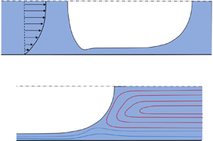
A typical set-up that is commonly used to study the dynamics of elongated bubbles is a horizontal capillary tube of radius  $R$, figure 1. In this setting, viscous forces and surface tension dominate over buoyancy and inertia. When the bubble translates at a constant speed, the gas takes a symmetrical bullet shape, commonly called a Taylor bubble, and a thin film of liquid is maintained between the bubble and the tube wall. Knowledge about the thickness of the film and its relationship with the bubble speed are crucial pieces of information for determining the transport rates in practical problems.

Figure 1. Sketch of the confined bubble that moves at speed  $U$ through a shear-thinning fluid in a channel of half-width $R$;
$R$;  $U_\infty$ is the average velocity far from the bubble. The shear-thinning fluid and the gaseous bubble are depicted in dark blue and white, respectively. The system of coordinates is placed on the right of the figure just for convenience: in the computation of the rear and front menisci the origin is somewhere in the region $CD$;
$CD$;  $AB$ and $EF$ are the spherical caps, $BC$ and $DE$ are the film regions, while $CD$ is the uniform film thickness region.
So far, a wide range of investigations have focused primarily on understanding the dynamics of a Taylor bubble in a Newtonian liquid. The first experiments of Fairbrother & Stubbs (Reference Fairbrother and Stubbs1935) and Taylor (Reference Taylor1961) suggested that the thickness of the lubricating film,  $h$, scales with the square root of the capillary number, $h/R= 0.5\,Ca^{1/2}$ , where $Ca=\mu U/\sigma$ is the capillary number and $U$,
$U$,  $\mu$, $\sigma$ and $R$ the bubble speed, the fluid viscosity, the surface tension and the pipe radius respectively. The seminal work of Bretherton (Reference Bretherton1961) demonstrated that $h/R= 1.34\,Ca^{2/3}$ in the limit of small $Ca$, as supported by several measurements (Schwartz, Princen & Kiss Reference Schwartz, Princen and Kiss1986; Aussillous & Quéré Reference Aussillous and Quéré2000). Thereafter, many researchers investigated the effect of finite capillary number and inertia (Cox Reference Cox1962; Reinelt & Saffman Reference Reinelt and Saffman1985; Aussillous & Quéré Reference Aussillous and Quéré2000; Heil Reference Heil2001; de Ryck Reference de Ryck2002; Khodaparast et al. Reference Khodaparast, Magnini, Borhani and Thome2015; Magnini et al. Reference Magnini, Ferrari, Thome and Stone2017), surfactants and variable surface tension, (Ratulowski & Chang Reference Ratulowski and Chang1990; Park Reference Park1992; Stebe & Barthés-Biesel Reference Stebe and Barthés-Biesel1995; Olgac & Muradoglu Reference Olgac and Muradoglu2013; Yu, Khodaparast & Stone Reference Yu, Khodaparast and Stone2017), unsteady flow, (Yu et al. Reference Yu, Zhu, Shim, Eggers and Stone2018), buoyancy, (Leung et al. Reference Leung, Gupta, Fletcher and Haynes2012; Atasi et al. Reference Atasi, Khodaparast, Scheid and Stone2017; Lamstaes & Eggers Reference Lamstaes and Eggers2017) and bubble viscosity, (Chen Reference Chen1986; Hodges, Jensen & Rallinson Reference Hodges, Jensen and Rallinson2004; Balestra, Zhu & Gallaire Reference Balestra, Zhu and Gallaire2018; Shukla et al. Reference Shukla, Kofman, Balestra, Zhu and Gallaire2019).
In many practical applications the working fluids exhibit a non-Newtonian behaviour (e.g. Savage et al. Reference Savage, Caggioni, Spicer and Cohen2010; Huisman, Friedman & Taborek Reference Huisman, Friedman and Taborek2012). Polymers solutions, suspensions, emulsions and biological fluids, just to mention a few, behave like shear-thinning fluids and, therefore, their viscosity is a function of the imposed shear rate. Specifically, at low shear rates, the shear stresses are proportional to the shear rate and the viscosity approaches a constant value, commonly known as the zero-shear-rate viscosity. At higher shear rates, instead, the viscosity decreases with increasing the shear rate, exhibiting a power-law behaviour. A decreasing viscosity can persist over several decades until, at very high shear rates, the viscosity flattens again, approaching the infinite-shear-rate viscosity. The latter limit is often not considered since fluid degradation may invalidate the rheological measurement, Bird, Armstrong & Hassager (Reference Bird, Armstrong and Hassager1987). Although such features are embedded in several viscosity models, e.g. the Carreau–Yasuda Carreau (Reference Carreau1972) and the Ellis models (Reiner Reference Reiner1965), the models available for describing the dynamics of a confined Taylor bubble in a shear-thinning fluid often ignore those limiting behaviours.
Existing studies on the topic assume that the liquid viscosity can be described by the power-law model (Kamişli & Ryan Reference Kamişli and Ryan1999, Reference Kamişli and Ryan2001; de Sousa et al. Reference de Sousa, Soares, de Queiroz and Thompson2007; Thompson, Soares & Bacchi Reference Thompson, Soares and Bacchi2010). The theory suggests that the lubricating film scales as  $h/R\sim {Ca}^{2/(2n+1)}_{*}$, where $n$ is the shear-thinning index and ${Ca}_{*}$ is a modified capillary number for power-law fluids. Unfortunately, the power-law model has an empirical nature and it does not accurately describe the viscosity at small shear rates, leading to large errors when applied to the multiphase scenario (Picchi et al. Reference Picchi, Poesio, Ullmann and Brauner2017, Reference Picchi, Barmak, Ullmann and Brauner2018a; Picchi, Ullmann & Brauner Reference Picchi, Ullmann and Brauner2018b). Both the local velocity field and integral variables (e.g. pressure drop and film thickness) are poorly predicted in free-surface flows due to the unrealistically and unbounded growth of the viscosity at small shear rates. This is confirmed by the work of Hewson, Kapur & Gaskell (Reference Hewson, Kapur and Gaskell2009) that studied the motion of a Taylor bubble through both power-law and an Ellis fluids. The power-law model generates inconsistencies in resolving the low-shear-rate regions of the velocity profile that can be overcome only accounting for the zero-shear-rate effect, see Hewson et al. (Reference Hewson, Kapur and Gaskell2009). Moreira et al. (Reference Moreira, Rocha, Carneiro, Araújo, Campos and Miranda2020) carried out numerical simulations of Taylor bubbles moving in a Carreau fluid at finite capillary numbers while Kawahara et al. (Reference Kawahara, Sadatomi, Law and Mansour2015) collected experimental data on a train of Taylor bubbles in shear-thinning polymer solutions. Also, lubricating films of shear-thinning liquids have been the subject of investigation in the context of the drag-out problem, i.e. the Landau & Levich (Reference Landau and Levich1942) problem, (Gutfinger & Tallmadge Reference Gutfinger and Tallmadge1965; Tallmadge Reference Tallmadge1966; Spiers, Subbaraman & Wilkinson Reference Spiers, Subbaraman and Wilkinson1975; Afanasiev, Münch & Wagner Reference Afanasiev, Münch and Wagner2007).
Other works focus on more complex non-Newtonian fluids. Mukundakrishnan, Ayyaswamy & Eckmann (Reference Mukundakrishnan, Ayyaswamy and Eckmann2008) studied numerically the motion of a gas bubble through a blood vessel and the blood is described as a Casson fluid; Zamankhan et al. (Reference Zamankhan, Helenbrook, Takayama and Grotberg2012) and Laborie et al. (Reference Laborie, Rouyer, Angelescu and Lorenceau2017) investigated yield-stress fluids. The effect of viscoelasticity was the subject of many theoretical and experimental works (Ho & Leal Reference Ho and Leal1975; Ro & Homsy Reference Ro and Homsy1995; Huzyak & Koelling Reference Huzyak and Koelling1997; Gauri & Koelling Reference Gauri and Koelling1999; Quintella, Souza Mendes & Carvalho Reference Quintella, Souza Mendes and Carvalho2007; Boehm, Sarker & Koelling Reference Boehm, Sarker and Koelling2011) including the studies on thin-film flows of viscoelastic fluids (e.g. Middleman Reference Middleman1978; Campanella, Galazzo & Cerro Reference Campanella, Galazzo and Cerro1986; de Ryck & Quéré Reference de Ryck and Quéré1998; Lee, Shaqfeh & Khomami Reference Lee, Shaqfeh and Khomami2002; Pasquali & Scriven Reference Pasquali and Scriven2002; Romero, Scriven & Carvalho Reference Romero, Scriven and Carvalho2006; Ashmore et al. Reference Ashmore, Shen, Kavehpour, Stone and McKinley2008; Bajaj, Ravi Prakash & Pasquali Reference Bajaj, Ravi Prakash and Pasquali2008).
However, in all the aforementioned studies, a generalized understanding of the bubble motion that embeds both the low- and high-shear-rate behaviours is still missing, including a generalization of the scaling laws for the film thickness and the bubble speed. To fill this gap, the goal of this paper is to study the dynamics of a confined Taylor bubble that moves in a shear-thinning fluid and to clarify the competition of the zero-shear-rate and the shear-thinning effects on bubble characteristics. We propose a theoretical framework that provides the scaling laws for the film thickness and the bubble speed and quantifies the interplay between low- and high-shear-rate behaviours. Our model generalizes Bretherton's results to shear-thinning fluids by identification of a universal scaling law for the effective viscosity and by proposing a generalization of capillary number that applies to both Newtonian and shear-thinning fluids. We also summarize the limitations of the power-law viscosity model discussing the extent to which its use can be legitimized.
With this aim, we derive a lubrication model for a Taylor bubble that moves in a shear-thinning fluid and whose viscosity is described by the Ellis viscosity model (§ 2). The Ellis model suits our scope since it allows for the derivation of the analytical velocity profile in the approximation of unidirectional free-surface flow. We show that the bubble meniscus obeys a third-order ordinary differential equation for the film thickness (§ 2.3). The model allows for the calculation of the front and rear menisci and the identification of the scaling laws for the film thickness, pressure drop and the bubble speed, see § 3. In § 3.2 we show that, if properly re-scaled, the effective viscosity can be described by a universal law that depends only on the two dimensionless numbers that describes the fluid rheology. Our results converge to Bretherton's theory in the Newtonian limit and we prove that the power-law viscosity model is not an accurate approximation in describing the bubble dynamics. The appearance of recirculating flow patterns ahead and behind the bubble is discussed in § 3.5, while pressure drops across the front and the rear menisci and the interfacial velocity in the film region are presented in Appendices B and C, respectively. The results obtained shed light on the mechanisms that control the motion of a Taylor bubble in a realistic shear-thinning fluid.
2. Theoretical derivation
2.1. Problem formulation
We consider a bubble confined in a horizontal planar channel that advances through a shear-thinning fluid as sketched in figure 1. The bubble is assumed inviscid and translates at a steady velocity  $U$ while, far from the bubble, the liquid moves with average velocity $U_\infty$. We assume that the bubble is sufficiently long so that a region with uniform film thickness $h$ exists and that gravity forces can be neglected. In other words, we assume that the macroscopic Bond number is sufficiently small, $Bo={\rm \Delta} \rho g R^2/\sigma \ll 1$ ( ${\rm \Delta} \rho$ and $g$ are the density difference and the gravitational acceleration, respectively). We start from the continuity and Navier–Stokes equations in the shear-thinning fluid without resolving the velocity field in the gas. We look at equations where inertial forces are unimportant in the thin film and the problem is controlled by the competition between viscous and surface tension forces only. The governing equations in the liquid are
 \begin{gather} \boldsymbol{\nabla} \boldsymbol{\cdot} {\boldsymbol{u}}= 0, \end{gather}
 \begin{gather}\rho \left[ \frac{\partial {\boldsymbol{u}}}{\partial {t}} +\left( {\boldsymbol{u}} \boldsymbol{\cdot} \boldsymbol{\nabla} \right){\boldsymbol{u}} \right]={-} \boldsymbol{\nabla} {p}+\boldsymbol{\nabla} \boldsymbol{\cdot} \boldsymbol{\tau}, \end{gather}
where  $p$ and $\boldsymbol {\tau }$ are the pressure and the shear stress tensor; $\boldsymbol {u}= (u,v)$ is the velocity vector with $u$ and $v$ representing the velocity components in the $x$ and $y$ directions, respectively. The boundary conditions are no slip and no penetration at the channel wall and a free shear-stress condition at the bubble–fluid interface.
The shear-thinning fluid is assumed to be an incompressible generalized Newtonian fluid of density  $\rho$ and effective viscosity $\mu$, whose constitutive relation can be formulated as
 \begin{equation} \boldsymbol{\tau}= \mu \boldsymbol{\dot{\gamma}}, \end{equation}
where  $\boldsymbol {\dot {\gamma }}=\boldsymbol{\nabla} \boldsymbol {u}+(\boldsymbol{\nabla} \boldsymbol {u})^\textrm {T}$ is the rate-of-strain tensor. Since we are interested in understanding the interplay between the shear-thinning and the zero-shear-rate effects on the bubble dynamics, we chose the Ellis viscosity model (Matsuhisa & Bird Reference Matsuhisa and Bird1965; Reiner Reference Reiner1965; Bird et al. Reference Bird, Armstrong and Hassager1987). The constitutive law of an Ellis fluid is given by
 \begin{equation} \mu=\frac{\mu_0}{1+({\tau}/{{\tau_{1/2}}})^{\alpha-1}}, \end{equation}
where  ${\tau }=\sqrt {1/2{(\boldsymbol {\tau }\boldsymbol {:}\boldsymbol {\tau })}}$ is the effective shear stress (or the magnitude of the shear-stress tensor). The model converges to Newtonian viscosity $\mu _0$, the zero-shear-rate viscosity, at small shear rates. The index $\alpha$ represents the degree of shear thinning and it assumes values $\alpha \in [1,\infty )$; the greater the value of $\alpha$, the greater is the extent of shear thinning. The constant $\tau _{1/2}$ controls the onset of the shear-thinning effect representing the effective shear stress at which the viscosity is 50 % of the Newtonian limit. The greater the value of $\tau _{1/2}$, the greater is the range of shear rates with the Newtonian viscosity. The Ellis model describes well the viscosity of many aqueous solutions (e.g. carboxymethyl cellulose and Carbopol solutions), where the typical values of the rheological constants are in the range $\alpha \in (1,3 )$ and $\tau _{1/2}= {\textit{O}}(10^{-3}\div 10)$, and the viscosity of many polymers, where $\alpha \in (1,4 )$ and $\tau _{1/2}= {\textit{O}}(1\div 10)$, see Bird et al. (Reference Bird, Armstrong and Hassager1987).
At high shear rates the shear-thinning effect dominates and (2.3) matches the power-law model (de Waele Reference de Waele1923; Ostwald Reference Ostwald1925)
 \begin{equation} \mu=\kappa {\dot{\gamma}}^{n-1}, \quad \textrm{with} \ \kappa=\mu_0^{n} \tau_{1/2}^{1-n} ,\quad n=1/\alpha, \end{equation}
where  $\dot {\gamma }=\sqrt {1/2 (\boldsymbol {\dot {\gamma }}\boldsymbol {:}\boldsymbol {\dot {\gamma }})}$ is the magnitude of the shear-rate tensor.
In the next section, we derive a lubrication model for a Taylor bubble when it reaches a steady state and moves along the tube with constant speed  $U$. Specifically, once formed, the uniform film thickness $h$ is constant with time in a reference frame that moves at the bubble speed $(x-Ut)$. This assumption is supported by the numerical simulations of Moreira et al. (Reference Moreira, Rocha, Carneiro, Araújo, Campos and Miranda2020) and the experiments of Kawahara et al. (Reference Kawahara, Sadatomi, Law and Mansour2015). Alternatively, in problems where the main interest is in characterizing the transient evolution of the bubble, one should derive an evolution equation for the film thickness in time (see for example Zhang & Lister Reference Zhang and Lister1999; Eggers & Fontelos Reference Eggers and Fontelos2015; Garg et al. Reference Garg, Kamat, Anthony, Thete and Basaran2017). In addition, we assume that the film thickness remains high enough to justify neglecting the effect of long-range intermolecular forces (e.g. van der Waals, disjoining pressure). Therefore, the possible rupture of the film and dewetting of the channel wall due to those destabilizing effects (see Zhang & Lister Reference Zhang and Lister1999; Diez & Kondic Reference Diez and Kondic2007; Garg et al. Reference Garg, Kamat, Anthony, Thete and Basaran2017) are out of the scope of this work.
2.2. Lubrication model
We consider the portions  $BC$ and $DE$ of the bubble in figure 1, where the curvature of the meniscus is established and the interface slope is small, $|\textrm {d}y_i/{\textrm {d} x}| \ll 1$, with $y_i$ denoting the location of the interface. The idea is to simplify the governing equations by introducing a small scaling parameter $\varepsilon$, defined as the ratio of the uniform film thickness $h$ to the unknown length of the film region along the flow direction, $h/\varepsilon$. This approach is typical of thin-film lubrication models (Eggers & Fontelos Reference Eggers and Fontelos2015) and, in the limit of $\varepsilon \ll 1$, it allows for the identification of the scaling laws in Landau–Levich–Derjaguin–Bretherton problems (see de Gennes, Brochard-Wyart & Quéré Reference de Gennes, Brochard-Wyart and Quéré2003; Stone Reference Stone2010).
Assuming that the velocity in the axial direction scales with the bubble speed  $U$, the following dimensionless variables are introduced
 \begin{equation} \tilde{x}=\frac{ x}{h/\varepsilon}, \quad \tilde{y}=\frac{y}{{h}}, \quad \tilde{u}=\frac{u}{{U}}, \quad \tilde{v}=\frac{v}{{V}}, \quad \tilde{t}=\frac{\varepsilon t}{h/U}, \quad \tilde{\mu}=\frac{\mu}{\mu_0},\quad \tilde{p}=\frac{p}{\sigma \varepsilon^2/h}, \end{equation}
where  $V$ is the characteristic scale of velocity in the $y$ direction. The continuity equation (2.1a) suggests that $V=\varepsilon U$, and we chose the zero-shear-rate viscosity $\mu _0$ as representative scale for the effective viscosity. The pressure in the film region scales with the normal pressure that can be estimated as $p\approx \sigma (\textrm {d}^2y_i/{\textrm {d} x}^2) \sim \sigma \varepsilon ^2/h$. Normalizing the momentum equations (2.1b) using (2.5) yields
 \begin{gather} \varepsilon Re \left[\frac{\partial \tilde{u}}{\partial \tilde{t}} + \tilde{u} \frac{\partial \tilde{u}}{\partial \tilde{x}} + \tilde{v} \frac{\partial \tilde{u}}{\partial \tilde{y}} \right] ={-} \frac{\varepsilon^3}{Ca} \frac{\partial \tilde{p}}{\partial \tilde{x}} + 2\varepsilon^2 \tilde{\mu}\frac{\partial \tilde{u}}{\partial \tilde{x}} + \frac{\partial }{\partial \tilde{y}} \left[ \tilde{\mu} \left( \frac{\partial \tilde{u}}{\partial \tilde{y}} + \varepsilon^2\frac{\partial \tilde{v}}{\partial \tilde{x}}\right)\right] , \end{gather}
 \begin{gather}\varepsilon Re \left[\frac{\partial \tilde{v}}{\partial \tilde{t}} + \tilde{u} \frac{\partial \tilde{v}}{\partial \tilde{x}} + \tilde{v} \frac{\partial \tilde{v}}{\partial \tilde{y}} \right] ={-} \frac{\varepsilon}{Ca} \frac{\partial \tilde{p}}{\partial \tilde{y}} + \frac{\partial }{\partial \tilde{x}} \left[ \tilde{\mu} \left( \frac{\partial \tilde{u}}{\partial \tilde{y}} + \varepsilon^2\frac{\partial \tilde{v}}{\partial \tilde{x}}\right)\right] + 2 \tilde{\mu} \frac{\partial \tilde{v}}{\partial \tilde{y}}, \end{gather}
where
 \begin{equation} Re = \frac{\rho U h}{{\mu_0}}, \quad {Ca} = \frac{{\mu_0} U}{\sigma}, \end{equation}
are the Reynolds and the capillary numbers both based on the zero-shear-rate viscosity.
Assuming that the scaling parameter is small,  $\varepsilon \ll 1$, and that inertial terms can be neglected, $\varepsilon Re \ll 1$, (2.6) simplifies to
 \begin{equation} 0 ={-} \frac{\varepsilon^3}{Ca} \frac{\partial \tilde{p}}{\partial \tilde{x}} + \frac{\partial}{\partial \tilde{y}}\left(\tilde{\mu}\frac{\partial \tilde{u}}{\partial \tilde{y}}\right). \end{equation}
Equation (2.9) shows that the viscous stress balances the axial pressure gradient only if  $\varepsilon ^3\approx Ca$ and, therefore, the $\tilde {x}$ variable can be expressed in terms of the capillary number as $\tilde {x}= x/{hCa^{-{1}/{3}}}$. This allows simplification of (2.7) to ${\partial \tilde {p}}/{\partial \tilde {y}}=0$, whereby the pressure is a function of the axial variable only. Note that the model is not applicable near the cap of the bubble where the curvature scales with the channel half-width $R$, and the slope of the interface is not small enough to justify the lubrication approximation. The effective shear stress reduces to
 \begin{equation} \tau=\sqrt{ \left[\tilde{\mu} \left( \frac{\partial \tilde{u}}{\partial \tilde{y}} + \varepsilon^2\frac{\partial \tilde{v}}{\partial \tilde{x}}\right) \right]^2 +2 \varepsilon^2 \left(\tilde{\mu}\frac{\partial \tilde{u}}{\partial \tilde{x}}\right)^2+2\varepsilon^2 \left( \tilde{\mu}\frac{\partial \tilde{v}}{\partial \tilde{y}}\right)^2 } \approx \left| \tilde{\mu} \frac{\partial \tilde{u}}{\partial \tilde{y}}\right|, \end{equation}
which is equal to the dimensionless shear stress in the film,  $\tilde {\tau }_{xy}\approx \tilde {\mu }{\partial \tilde {u}}/{\partial \tilde {y}}$. The corresponding effective viscosity can be written as
 \begin{equation} \tilde{\mu} = \frac{1}{1+{(|\tilde{\tau}_{xy}}|/{El})^{\alpha-1}} \quad \textrm{with} \ El=\frac{\tau_{1/2}h}{U\mu_0}=\frac{\tau_{1/2}/\mu_0}{U/h}, \end{equation}
where  $El$ is the Ellis number. The Ellis number can be interpreted as the ratio between the characteristics shear rate of the fluid, $\tau _{1/2}/\mu _0$, and the representative shear rate in the film, $U/h$. When $El\rightarrow \infty$ the onset of the shear-thinning effect is delayed to an infinite shear rate and the model reduces to a Newtonian fluid of viscosity $\mu _0$ (and $\tilde {\mu }=1$), figure 2(a). We refer to this case as the Newtonian limit. Instead, when the shear rate is sufficiently high, or $El$ is small such that the Newtonian plateau shrinks to extremely low shear rates, the shear-thinning effects dominates in (2.11) and the viscosity matches that of a power-law fluid with a slope $(1-\alpha )/\alpha$, figure 2. As $\alpha \rightarrow 1$ the fluid exhibits a power-law behaviour almost in the entire range of shear rates, while for $\alpha =1$, $\tilde {\mu }=1/2$.

Figure 2. Dimensionless effective viscosity  $\tilde {\mu }=\mu /\mu _0$ as a function of the dimensionless shear rate, the Ellis number, $El$ and the degree of shear thinning, $\alpha$: (a) $\alpha =2$; (b) $El=0.1$. The power-law limit is also plotted (red-dashed line).
At the interface we ensure the continuity of normal and tangential stresses and the boundary conditions read
 \begin{gather} -\tilde{p}|_\eta + \left.2 {Ca}\, \varepsilon^{{-}1} \tilde{\mu}\frac{\partial \tilde{v}}{\partial \tilde{y}}\right|_\eta = \frac{ \left.\dfrac{\partial^2 \eta}{\partial \tilde{x}^2}\right|_\eta }{\left[ 1+\varepsilon^2\left(\left.\dfrac{\partial \eta}{\partial \tilde{x}}\right|_\eta \right)^2 \right]^{3/2}} , \quad \textrm{with} \ \eta=\frac{y_i}{h}, \end{gather}
 \begin{gather}\left. \frac{\partial \tilde{u}}{\partial \tilde{y}} \right|_\eta = 0. \end{gather}
Since  $Ca\approx \varepsilon ^3$ and $\varepsilon \ll 1$, (2.12) further simplifies to
 \begin{equation} -\tilde{p}|_\eta = \left.\frac{\partial^2 \eta}{\partial \tilde{x}^2}\right|_\eta. \end{equation}
The assumption that  $\varepsilon \ll 1$ implies that the slope of the interface in the film region is small, namely $d\eta /{\rm d} \tilde {x} \ll Ca^{-1/3}$. A formulation of the boundary condition that relaxes this constraint is discussed in Park & Homsy (Reference Park and Homsy1984) and Reinelt (Reference Reinelt1987).
2.3. Film equation
We integrate (2.9) subjected to (2.13) at  $\tilde {y}=\eta$ and the no-slip condition at $\tilde {y}=0$ to obtain the (instantaneous) velocity profile of shear-thinning fluid
 \begin{equation} \tilde{u}(\tilde{y}) = \frac{1}{2}\frac{\textrm{d}\tilde{p}}{\textrm{d}\tilde{x}}( \tilde{y}^2 - 2\eta \tilde{y}) + \frac{1}{(\alpha+1) El^{\alpha-1}}\frac{\textrm{d}\tilde{p}}{\textrm{d}\tilde{x}} \left|\frac{\textrm{d}\tilde{p}}{\textrm{d}\tilde{x}}\right|^{\alpha-1} [ (\eta - \tilde{y} )^{\alpha+1} - \eta^{\alpha+1}], \end{equation}
where  $\tilde {y}\in [0,\eta ]$. The velocity profile is composed by a Newtonian and a shear-thinning parts, reflecting the structure of the Ellis rheological model that can be seen as the sum of a Newtonian and a power-law viscosity model, see Gutfinger & Tallmadge (Reference Gutfinger and Tallmadge1965). The details concerning the derivation of the velocity profile are listed in Appendix A. Then, we compute the volume flux by integrating the velocity profile (2.15) over the film thickness
 \begin{equation} \tilde{Q} = \int_0^\eta \tilde{u}(\tilde{y})\, {\rm d} \tilde{y} ={-}\frac{1}{3}\frac{\textrm{d}\tilde{p}}{\textrm{d}\tilde{x}}\eta^3 - \frac{1}{(\alpha+2) El^{\alpha-1}} \frac{\textrm{d}\tilde{p}}{\textrm{d}\tilde{x}} \left|\frac{\textrm{d}\tilde{p}}{\textrm{d}\tilde{x}}\right|^{\alpha-1} \eta^{\alpha+2}, \end{equation}
where  $\tilde {Q}=Q/hU$ with $Q$ the dimensional flux in the film.
Looking at the problem from a reference frame moving with the bubble at the speed  $U$, the mass balance between the region of uniform thickness $CD$ and the film region $CB$ (see figure 1) yields
 \begin{equation} (0-U)h=(Q/y_i-U)y_i. \end{equation}
In the region  $CD$ the liquid is at rest since $\eta =1$ and the pressure is constant from (2.14). In terms of dimensionless coordinates, (2.17) becomes
 \begin{equation} \tilde{Q} = \eta -1. \end{equation}
Combining (2.16) and (2.18) and using the boundary condition (2.14) to express the driving force,  ${\rm d} \tilde {p}/{\rm d} \tilde {x}=-{\rm d} ^3\eta /{\rm d} \tilde {x}^3$, we obtain
 \begin{equation} \frac{\textrm{d}^3\eta}{{\rm d} \tilde{x}^3} + \frac{3}{(\alpha + 2)El^{\alpha -1}}\frac{\textrm{d}^3\eta}{{\rm d} \tilde{x}^3}\left|-\frac{\textrm{d}^3\eta}{{\rm d}\tilde{x}^3}\right|^{\alpha-1} \eta^{\alpha-1}= 3 \frac{\eta - 1}{\eta^3}. \end{equation}
Defining  $\xi = 3^{1/3}\tilde{x}=x/[h(3Ca)^{-1/3}]$ we finally get the following ordinary differential equation for $\eta$
 \begin{equation} \underbrace{\frac{\textrm{d}^3\eta}{{\rm d} \xi^3}}_{\mathcal{I}} + \underbrace{\frac{3^\alpha}{(\alpha + 2)El^{\alpha -1}}\frac{\textrm{d}^3\eta}{{\rm d} \xi^3}\left|-\frac{\textrm{d}^3\eta}{{\rm d} \xi^3}\right|^{\alpha-1} \eta^{\alpha-1}}_{\mathcal{II}}= \frac{\eta - 1}{\eta^3}, \end{equation}
where the bubble profile  $\eta$ is a function of $\xi$, $\alpha$ and $El$ only. Equation (2.20) describes the meniscus between the uniform film and the caps at both the bubble ends in a moving reference frame $(x-Ut)$. The left-hand side of (2.20) is composed of a Newtonian and a shear-thinning term, indicated as $\mathcal {I}$ and $\mathcal {II}$, respectively.
When the  $\mathcal {II}$ becomes negligible, (2.20) converges to the classical result obtained by Bretherton (Reference Bretherton1961) for a Newtonian liquid,
 \begin{equation} \frac{\textrm{d}^3\eta}{{\rm d} \xi^3} = \frac{\eta - 1}{\eta^3}. \end{equation}
We recover the Newtonian liquid either for  $El\rightarrow \infty$, or for specific combinations of $El$ and $\alpha$ so that the shear-thinning effect vanishes, see figure 2. Also, when the third derivative goes to zero, ${\rm d} ^3\eta /{\rm d} \xi ^3\rightarrow 0$, (2.20) reduces to (2.21), as it will be discussed in detail in § 3.1. If we artificially remove the term $\mathcal {I}$ from (2.20), we recover the equation for a power-law fluid
 \begin{equation} \frac{\textrm{d}^3\eta}{{\rm d} \xi^3}\left|-\frac{\textrm{d}^3\eta}{{\rm d} \xi^3}\right|^{\alpha-1} = \frac{(\alpha + 2)^{{1}/{\alpha}}El^{({\alpha -1})/{\alpha}}}{3} \frac{(\eta - 1)}{\eta^{{2+\alpha}}}. \end{equation}
Equation (2.22) holds only when the shear-thinning term dominates and, assuming that  ${\rm d} ^3\eta /{\rm d} \xi ^3\geq 0$, i.e. considering the front of the bubble only, (2.22) is equivalent to the one derived by Kamişli & Ryan (Reference Kamişli and Ryan1999, Reference Kamişli and Ryan2001) for power-law fluids. Although mathematically correct, the model for power-law fluid leads to non-physical results when integrated starting from the uniform thickness region and the extent to which its use could be legitimized will be discussed in § 3.1.
The general solution of (2.20) can be found numerically starting from the region  $CD$ and integrating in the directions of the front and rear menisci. To do that, it is convenient to discuss few limiting cases where the solution can be obtained analytically (§ 2.4).
2.4. Scaling of the film equation
In regions near  $C$ and near $D$ the film thickness approaches a uniform value ( $y_i\simeq h$) and we can write
 \begin{equation} \eta \approx 1+ \eta_1+\cdots\quad \textrm{with}\ \eta_1 \ll 1. \end{equation}
Upon substituting (2.23) into (2.20) we obtain
 \begin{equation} \frac{\textrm{d}^3 \eta_1}{{\rm d} \xi^3} +\textrm{sign}\left(\frac{\textrm{d}^3 \eta_1}{{\rm d} \xi^3}\right)\frac{3^\alpha }{(\alpha+2)El^{\alpha-1}} (1+\eta_1)^{\alpha-1} \left|- \frac{\textrm{d}^3 \eta_1}{{\rm d} \xi^3} \right|^\alpha=\frac{\eta_1}{(1+\eta_1)^3}. \end{equation}
Expanding the two binomials in (2.24) into Taylor series, truncating after the second term and recalling that  $\eta _1=\eta -1$, we obtain an approximation of the film equation near the uniform film
 \begin{equation} \frac{\textrm{d}^3 \eta}{{\rm d} \xi^3} +\textrm{sign}\left(\frac{\textrm{d}^3 \eta_1}{{\rm d} \xi^3}\right)\frac{3^\alpha }{(\alpha+2)El^{\alpha-1}} \left|- \frac{\textrm{d}^3 \eta}{{\rm d} \xi^3} \right|^\alpha = \eta-1 \quad \textrm{for} \ \eta\simeq 1. \end{equation}
If  $\textit{O}( 3^\alpha |{\rm d} ^3 \eta /{\rm d} \xi ^3|^{\alpha }/ (\alpha +2)El^{\alpha -1} ) \ll 1$, (2.25) reduces to
 \begin{equation} \frac{\textrm{d}^3 \eta}{{\rm d} \xi^3} = \eta -1 \quad \textrm{for} \ \eta\simeq 1, \end{equation}
and it admits an analytical solution
 \begin{equation} \eta=1+ae^{\xi}+be^{-\xi/2}\cos{\left(\frac{\sqrt{3}}{2}\xi\right)} +ce^{-\xi/2}\sin{\left(\frac{\sqrt{3}}{2}\xi\right)}, \end{equation}
where  $a$,
$a$,  $b$,
$b$,  $c$ are constants. This is the same approximation valid for Newtonian fluids and it holds also for an Ellis fluid since the third derivative in this region is small, ${\rm d} ^3 \eta /{\rm d} \xi ^3\ll 1$; this assumption will be justified a posteriori in § 3.1. In the following, we refer to portions of the bubble where (2.27) applies as the exponential regions, see figure 3.

Figure 3. Numerical solution (red), the exponential initial condition (dashed black) and the parabolic region for  $El=1$ and $\alpha =2$ for the (a) bubble front, (b) bubble rear. The solutions have been shifted along $\xi$ to ensure that the coefficient $Q$ in (2.29) is $Q=0$ .
In regions where  $\eta \gg 1$ and the slope of the interface is small enough, $dy_i/{\textrm {d} x}\ll 1$ (or, in terms of dimensionless variables $d\eta /{\rm d} \xi \ll Ca^{-1/3}$), so that the lubrication approximation holds, (2.20) reduces to
 \begin{equation} \frac{\textrm{d}^3\eta}{{\rm d} \xi^3}\approx 0 \quad \textrm{with} \ \eta\gg1. \end{equation}
Integration yields a parabolic behaviour with respect to  $\xi$
$\xi$
 \begin{equation} \eta=\frac{P}{2}\xi^2+W\xi+Z, \end{equation}
where  $P$,
$P$,  $W$ and $Z$ are constants to be determined from the numerical solution of (2.20), see § 2.5. Specifically, the coefficient $P$ is the dimensionless curvature of the meniscus when $\eta \gg 1$, i.e. the second derivative of $\eta$ with respect to $\xi$, $P={\rm d} ^2\eta /{\rm d} \xi ^2$. Given $El$ and $\alpha$, the value of $P$ can be obtained from the numerical solution far from the uniform film region for both the front and the rear menisci. The determination of the coefficients $W$ and $Z$ requires numerical fitting: $W$ is made zero by shifting the solution along $\xi$, while $Z$ is fitted from a window that gives, in the Newtonian limit, the same value obtained by Bretherton (Reference Bretherton1961) ( $Z=2.79$ in the front and $Z=-0.72$ in the rear). The portions of the bubble where (2.29) applies are referred as the parabolic regions, see figure 3.
2.5. Boundary conditions and numerical solution
The film shape between the uniform film and the caps at both ends is obtained by solving (2.20) using the fully implicit solver ode15i of Matlab. The front and the rear menisci are treated separately integrating (2.20) with a different set of boundary conditions.
The front meniscus is obtained by integrating (2.20) starting from somewhere near  $C$ (figure 1) towards positive $\xi$. We chose to set the origin at $\xi =0$, assuming that the uniform film region extends to $\xi \rightarrow - \infty$, or, alternatively, that $\eta (-\infty )=1$. This means that, near $C$, we can approximate the solution with the exponential approximation (2.27). In the front, the cosine and sine terms in (2.27) are small due to the damping effect of the negative exponentials, and (2.27) can be simplified as
 \begin{equation} \eta \simeq 1+ae^{\xi}. \end{equation}
For specified values of  $El$ and $\alpha$, the solution is unique. Starting the integration from $\xi =0$ we set $a=10^{-5}$ and
 \begin{equation} \eta(0)=1+a, \quad \left.\frac{\textrm{d} \eta}{{\rm d} \xi}\right|_0=a, \quad \left.\frac{\textrm{d}^2 \eta}{{\rm d} \xi^2}\right|_0=a, \quad \left.\frac{\textrm{d}^3 \eta}{{\rm d} \xi^3}\right|_0=a. \end{equation}
Different values of  $a$ result only in a shift in the origin of $\xi$. The (translated) front profile is shown in figure 3(a). The exponential solution is also plotted indicating that, as $\xi$ increases, the numerical solution diverges from (2.30).
The profile in the rear meniscus is obtained by integrating (2.20) towards negative  $\xi$ starting from the boundary condition $\eta (\infty )=1$. Near $D$, we can approximate the solution with the exponential function (2.27) that, for negative $\xi$, can be simplified neglecting the positive exponential as
 \begin{equation} \eta \simeq 1+be^{-\xi/2}\cos{\left(\frac{\sqrt{3}}{2}\xi\right)} +ce^{-\xi/2}\sin{\left(\frac{\sqrt{3}}{2}\xi\right)}. \end{equation}
Choosing  $\xi =0$ as the origin we get
 \begin{equation} \eta(0)=1+b, \quad \left.\frac{\textrm{d} \eta}{{\rm d} \xi}\right|_0=c\frac{\sqrt{3}}{2}-\frac{b}{2}, \quad \left.\frac{\textrm{d}^2 \eta}{{\rm d} \xi^2}\right|_0={-}\frac{b}{2}-c\frac{\sqrt{3}}{2}, \quad \left.\frac{\textrm{d}^3 \eta}{{\rm d} \xi^3}\right|_0=b. \end{equation}
In (2.33a–d) there are two disposable constants:  $b$ has the effect of shifting the origin of the bubble profile only and we arbitrarily set the value to $b=10^{-4}$. The other constant determines the curvature of the menisci at $\eta \gg 1$, i.e. for $\xi \rightarrow -\infty$. It is a common choice to assume that the curvature in the rear matches the one in the front, see Bretherton (Reference Bretherton1961), imposing
 \begin{equation} \left. \frac{\textrm{d}^2 \eta_{rear}}{{\rm d} \xi^2}\right|_{\xi \rightarrow -\infty}= \left. \frac{\textrm{d}^2 \eta_{front}}{{\rm d} \xi^2}\right |_{\xi \rightarrow + \infty}. \end{equation}
The boundary condition is satisfied by an iterative loop on the constant  $c$ in (2.33a–d); this loop imposes that the second derivative – the curvature – of $\eta$ in the parabolic region equals the one of the front meniscus calculated for given values of $El$ and $\alpha$. A plot of the calculated rear meniscus is given in 3(b). Differently from the front meniscus that is monotonic, the rear meniscus develops the typical oscillations. A discussion about the relaxation of the boundary condition (2.34) is given in Appendix D.
3. Results and discussion
3.1. Characteristics of the front meniscus
We compute the front meniscus as described in § 2.5 aiming at exploring the effect of the rheology of the shear-thinning liquid on bubble characteristics. Differently from the Newtonian case, where the profile is uniquely determined by the dimensionless variables  $\eta$ and $\xi$, here, the profile also depends on $El$ and $\alpha$.
The Ellis number controls the onset of the shear-thinning effect. When  $El \rightarrow \infty$, the front meniscus converges to the Newtonian limit and the problem does not depend anymore on $\alpha$, figure 4(a). Instead, as $El$ decreases, the Newtonian plateau in the viscosity curve shrinks, see figure 2(a), and the dimensionless curvature of the meniscus ${\rm d} ^2\eta /{\rm d} \xi ^2$ when $\eta \gg 1$ decreases, see figure 4(b). The change in the meniscus shape is an effect of the local variation in the effective viscosity of the liquid, as demonstrated in figure 5. The effective viscosity $\tilde {\mu }|_w$ is computed using (2.11) based on the shear rate at the channel wall ( $\tilde {y}=0$) defined as
 \begin{equation} \left. \frac{\textrm{d} \tilde{u}}{\textrm{d}\tilde{y}}\right |_w={-} \frac{\textrm{d}\tilde{p}}{\textrm{d}\tilde{x}}\eta-{El^{1-\alpha}}\frac{\textrm{d}\tilde{p}}{\textrm{d}\tilde{x}}\left|\frac{\textrm{d}\tilde{p}}{\textrm{d}\tilde{x}}\right| ^{\alpha-1} \eta^\alpha . \end{equation}
In the vicinity of the uniform thickness region, the effective viscosity is  $\tilde {\mu }|_w=1$ since the fluid is at rest. This means that we can always identify a region of the bubble where the liquid exhibits a Newtonian behaviour. The existence of a high (Newtonian) viscosity region within the uniform film thickness is indeed confirmed by the viscosity field obtained from numerical simulations by Moreira et al. (Reference Moreira, Rocha, Carneiro, Araújo, Campos and Miranda2020). To quantify the shear-thinning effect, the weights of the Newtonian and shear-thinning terms are plotted in figure 5 as
 \begin{equation} \mathcal{I}_N=\frac{\mathcal{I}}{\mathcal{I}+\mathcal{II}}, \quad \mathcal{I}_{PL}=\frac{\mathcal{II}}{\mathcal{I}+\mathcal{II}}, \end{equation}
where  $\mathcal {I}$ and $\mathcal {II}$ refers to (2.20). For $El=10$ the shear-thinning term is negligible over the entire meniscus and the profile is almost indistinguishable from a Newtonian profile. Instead, for $El=1, 10^{-1}, 10^{-5}$ we can identify a region of the bubble where the shear-thinning term in (2.20) is comparable to the Newtonian one, figure 5(c), or entirely dominates the solution, figure 5(d). We define the shear-thinning region (depicted in grey) when $\mathcal {I}_N\leq 0.95$.

Figure 4. Bubble meniscus at the front, (a) and dimensionless curvature, (b), as a function of the Ellis number for a shear-thinning fluid with  $\alpha =2$.

Figure 5. Front meniscus and effective viscosity computed based on the shear rate at the wall for a shear-thinning fluid with  $\alpha =2$ and (a) $El=10$; (b) $El=1$; (c) $El=10^{-1}$; (d) $El=10^{-5}$. The Newtonian region (white) and the shear-thinning region (grey) are highlighted. The insets show the weight of the Newtonian, $\mathcal {I}_N$, and the shear-thinning, $\mathcal {I}_{PL}$, terms in (2.20).
The terms (3.2a,b) suggest that the shear-thinning effect is important only when the film starts growing rapidly before entering the parabolic region. There, the shear rate has a maximum that corresponds to a minimum in the effective viscosity. As expected, the lower  $El$ is, the lower is the minimum of $\tilde {\mu }|_w$. Far from the uniform thickness region where $\eta$ is large, the third derivative ${\rm d} ^3\eta /{\rm d} \xi ^3\rightarrow 0$ and, as a consequence, the effective viscosity reduces rapidly, see (3.1). Although this would imply the tendency of reaching the Newtonian limit again, we remind that the model is not applicable too far from the region $CD$.
$CD$.
The fact that the shear-thinning effect arises only in a small portion of the bubble indicates that the use of the power-law model for describing the meniscus is physically incorrect. In particular, since in the vicinity of the uniform film region, the problem is dominated by the Newtonian term (figure 5), the integration of (2.22) would lead to non-physical results. The power-law effective viscosity would grow to the infinite near the origin since  ${\rm d} \tilde {u}/{\rm d} \tilde {y}\approx 0$. The choice made by Kamişli & Ryan (Reference Kamişli and Ryan1999) of solving (2.22) starting from a Newtonian initial condition, but not accounting for the Newtonian term, does not seem a correct representation of the physics of the problem.
The shear-thinning effect also delays the transition to the parabolic region that is characterized by a constant dimensionless curvature and  ${\rm d} ^3\eta /{\rm d} \xi ^3 \approx 0$, see § 2.4. As $El$ decreases, the starting point of the parabolic region shifts to higher $\xi$, as can be seen by analysis of the rate at which the third derivative approaches a zero value. In the Newtonian limit,
 \begin{equation} \lim_{\eta \rightarrow \infty} \frac{\textrm{d}^3 \eta}{{\rm d} \xi^3}=\lim_{\eta \rightarrow \infty}\frac{1}{\eta^2}\rightarrow 0, \end{equation}
the third derivative in (2.21) decays proportionally to  $1/\eta ^2$. In case the shear-thinning effect dominates, such as for $El=10^{-5}$ in figure 5(d), the third derivative in (2.22) decays proportionally to $1/\eta ^{({1+\alpha })/{\alpha }}$,
 \begin{equation} \lim_{\eta \rightarrow \infty} \frac{\textrm{d}^3 \eta}{{\rm d} \xi^3}=\lim_{\eta \rightarrow \infty}\frac{(\alpha+2)^{{1}/{\alpha}}El^{({\alpha-1})/{\alpha}}}{3} \frac{1}{\eta^{({1+\alpha})/{\alpha}}}\rightarrow 0. \end{equation}
Since  $\alpha >1$, the onset of the parabolic region is delayed.
Changes in the degree of shear thinning  $\alpha$ result in two different behaviours. When the shear rate is smaller than 0.2 (the value at which $\tilde {\mu }=1/2$), the system tends to the Newtonian limit for $\alpha \rightarrow \infty$. Instead, when the shear rate is greater than 0.2, an increase in $\alpha$ translates in a decrease of the effective viscosity, see figure 2(b). Accordingly, in figure 6, the front meniscus approaches the Newtonian limit for $El=1$ while it shows the opposite behaviour for $El=10^{-2}$. Since the effective shear rate of the problem scales as $\dot {\gamma }_e\sim 1/El$, the two opposing behaviours depend on whether the Ellis number is greater or smaller of a critical value. For $\alpha =1$ we recover a Newtonian fluid with $\tilde {\mu }=1/2$ and the meniscus is identical to the one obtained in the Newtonian limit with a change of variables $\xi ^*=\xi /\sqrt [3]{2}$.

Figure 6. Effect of the degree of shear thinning  $\alpha$ on the shape of front meniscus for (a) $El=1$ ; (b) $El=10^{-2}$.
The characteristics of the front meniscus can be summarized looking at the scaling behaviour of the coefficients in the parabolic solution (2.29). Figure 7(a) shows  $P$ as a function of $El$ and $\alpha$. When $El\rightarrow \infty$ all the curves approach the Newtonian limit and $P= 0.643$ as obtained by Bretherton (Reference Bretherton1961). The curvature of the Newtonian limit is the maximal curvature that the meniscus can assume. As $El\rightarrow 0$, instead, the curvature decreases significantly and, when $\alpha \rightarrow 1$, the shear-thinning effect delays the transition to the Newtonian limit to much higher $El$. Figure 7(b) shows the trends for the coefficient $Z$ in (2.29).

Figure 7. Coefficients  $P$ and $Z$ in (2.29) that characterize the front meniscus in the parabolic region as a function of the Ellis number and the degree of shear thinning $\alpha$. Note that the coefficient $P$ is also the dimensionless curvature of the meniscus for $\eta \gg 1$, $P={\rm d} ^2\eta /{\rm d} \xi ^2$.
3.2. Scaling of the film thickness and generalization of the capillary number
The model for the film thickness is obtained by matching the curvature of the parabolic region near  $B$ with the curvature of the spherical cap $AB$, see figure 1. Specifically, near $B$ the curvature is constant
 \begin{equation} \frac{\textrm{d}^2 y_i}{{\textrm{d} x}^2}=\frac{P}{h} (3\, Ca)^{2/3}, \end{equation}
while in the spherical cap the curvature scales as  ${\rm d} ^2 y_i/{\textrm {d} x}^2\sim 1/R$. By matching the two curvatures we obtain
 \begin{equation} \frac{h}{R}= P (3\, Ca)^{2/3}, \end{equation}
where  $P(El,\alpha )$ is a function of the Ellis number and $\alpha$ only. Differently from the Newtonian case, the film thickness is determined by the interplay of three dimensionless numbers, $h(Ca,El,\alpha )$, and it converges to the correlation proposed by Bretherton (Reference Bretherton1961) in the Newtonian limit. The scaling law for $h/R$ is summarized in figure 8. The film thickness decreases with decreasing of the Ellis number since the effective viscosity of the problem diminishes, figure 8(a). Therefore, when the shear-thinning effect dominates (i.e. low $El$), the bubble forms a thinner film compared with a Newtonian fluid with the same capillary number. Variations in the degree of shear thinning $\alpha$ produce two opposite behaviours depending on whether the effective shear rate (or $1/El$) exceeds the critical value, see 8(b,c).

Figure 8. (a–c) Dimensionless film thickness,  $h/R$, as a function of the capillary number, $Ca$, the Ellis number, $El$, and the degree of shear thinning, $\alpha$.
The model for the film thickness (3.6) is still based on the definition of the capillary number defined with the zero-shear-rate viscosity, see (2.8a,b). It would be desirable to obtain a formulation of the capillary number that embeds both the zero-shear-rate and the shear-thinning effects. With this aim, we can recast (3.6) in the following form introducing the effective capillary number  $Ca_e$
 \begin{equation} \frac{h}{R}= 0.643 (3\, Ca_{e})^{2/3} \quad \textrm{with} \ Ca_{e}=\frac{\mu_eU}{\sigma}, \end{equation}
where  $\mu _e$ is the effective viscosity defined as
 \begin{equation} {\mu_e}=\mu_0 \left(\frac{P}{0.643}\right)^{{3}/{2}}. \end{equation}
A plot of the effective viscosity as a function of the effective shear rate  $1/El$ is provided in figure 9(a). Since the determination of $P$ requires the numerical solution of (2.20), we use the numerical results to get a fitting curve for the effective viscosity. The data of figure 9(a) collapse over the same master curve, figure 9(b), if we define
 \begin{equation} \frac{\mu_e}{\mu_0}= \left\{ \begin{array}{@{}ll} 1, & \textrm{if} \ El \rightarrow \infty, \\ 0.725 \dfrac{17\alpha-12 }{5\alpha}{{El}^{{(\alpha-1)}/{\alpha}}} , & \textrm{if} \ El \rightarrow 0. \end{array} \right. \end{equation}
The scaling law for  $El\rightarrow 0$ has been inspired by the definition of the effective viscosity for a power-law fluid
 \begin{equation} \tilde{\mu}= \tilde{\kappa} ( \dot{\gamma}_e )^{({1-\alpha})/{\alpha}} \quad \textrm{with} \ \dot{\gamma}_e \sim \frac{1}{El}, \end{equation}
where  $\tilde {\kappa }=0.725(17\alpha -12)/5\alpha$ and $n=1/\alpha$. Equation (3.9) is the universal scaling for the effective viscosity for a confined Taylor bubble that moves in a shear-thinning liquid and it allows for the definition of a generalized capillary number for the problem.

Figure 9. (a) Effective viscosity as a function of the effective shear rate,  $1/El$, and the degree of shear thinning $\alpha$. (b) Collapsing of all the viscosity curves around the master curve (3.9).
The trends of figure 8 are in a qualitative agreement with the simulations of Moreira et al. (Reference Moreira, Rocha, Carneiro, Araújo, Campos and Miranda2020). In particular, the film thickness decreases with increasing of the degree of shear thinning at a fixed capillary number. Unfortunately, their data cannot be used to validate our model since the flow rates necessary to define the capillary number are not reported in the manuscript. Also, the data collected by Kamişli & Ryan (Reference Kamişli and Ryan1999) and by Kawahara et al. (Reference Kawahara, Sadatomi, Law and Mansour2015) cannot be considered to validate the scaling law for the film thickness because the rheological data do not include the low-shear-rate behaviour and only the power-law behaviour has been provided. For a complete validation of our model, more experiments or simulations performed with realistic shear-thinning fluids would be valuable and are encouraged.
3.3. Bubble speed
A measure of the ratio between the bubble speed  $U$ and the average velocity of the fluid ahead of the bubble $U_\infty$ is a critical parameter in the design of many applications that involve bubbles and trains of bubbles. We can derive the scaling law for $U/U_\infty$ applying the mass balance to the problem. Specifically, if we write the balance between the open tube and the uniform film region in a reference frame that moves with the bubble speed $U$
$U$
 \begin{equation} (0-U)h=(U_\infty-U)R, \end{equation}
we obtain
 \begin{equation} \frac{U_\infty}{U}=1-\frac{h}{R}. \end{equation}
Combining (3.12) with (3.6) or (3.7) we obtain the scaling law valid for the two-plate geometry
 \begin{equation} \frac{U}{U_\infty}=\frac{1}{1-P (3\, Ca)^{2/3}}=\frac{1}{1-(3Ca_e)^{2/3}}. \end{equation}
The bubble always flows faster compared with the fluid ahead from the bubble,  $U/U_\infty >1$, and, only in the limit of $Ca\rightarrow 0$, the speed of the bubble is almost indistinguishable from $U_\infty$, see figure 10. In general, when the shear-thinning effect plays a role (i.e. low $El$), the bubble flows slowly compared with a Newtonian bubble with the same capillary number $Ca$. The lower the effective viscosity is, the slower is the bubble compared with $U_\infty$. The effect of $\alpha$ is summarized in figure 10(b,c), where we see that increasing the degree of shear thinning can increase the bubble velocity at $El=1$. As expected the scaling law for $U/U_\infty$ converges to the one obtained by Bretherton (Reference Bretherton1961) for $El\rightarrow \infty$. The trends of figure 10 are in a qualitative agreement with the simulations of Moreira et al. (Reference Moreira, Rocha, Carneiro, Araújo, Campos and Miranda2020) where the bubble speed decreases with increasing of the degree of shear thinning at a fixed capillary number.

Figure 10. (a–c) Ratio of the bubble speed to the average velocity of the fluid ahead of the bubble,  $U/U_\infty$, as a function of the capillary number, $Ca$, the Ellis number, $El$, and the degree of shear thinning, $\alpha$. (d) Value of $U/U_\infty$ as a function of the generalized capillary number, $Ca_e$, for the planar two-plate geometry (the case solved in this work) and its extension to the pipe geometry.
Using the definition of the generalized capillary number  $Ca_e$ defined in § 3.2, the ratio $U/U_\infty$ is monotonic with $Ca_e$ and all the curves collapse on the same one depicted in 10(d). This analysis can be generalized to the case of a pipe geometry by referring to the film holdup instead of the film thickness in (3.11). In the case of circular geometry, the film holdup scales with $\sim [ 1-(1-h/R)^2]$ yielding
 \begin{equation} \frac{U}{U_\infty}=\frac{1}{[1-P (3\, Ca)^{2/3}]^2}=\frac{1}{[1-(3Ca_e)^{2/3}]^2}. \end{equation}
In figure 10(d) we can see that the speed ratio  $U/U_\infty$ attains a higher value in a pipe compared with the two-plate geometry.
3.4. Characteristics of rear meniscus and limitations of the lubrication approximation
We compute the profile of the rear meniscus as described in § 2.5. In terms of the curvature far from the uniform film region, the rear meniscus resembles the same trends of the bubble front, see figure 11. The main difference is the presence of oscillations in the bubble profile that stretches along  $\xi$ as the shear-thinning effect becomes more important. As the curvature $P$ decreases, the minimum of the profile shifts closer to the channel wall. $\mathcal {I}_N$ and $\mathcal {I}_{PL}$ show that, similarly to the front, the region in the vicinity of the uniform film thickness is dominated by the Newtonian term. Instead, there is a competition between the two near the minimum of the profile, while at $\xi \rightarrow -\infty$, the shear-thinning term decays and the problem converges again to the Newtonian one.

Figure 11. (a) Rear meniscus as a function of the Ellis number for a shear-thinning fluid with  $\alpha =2$. (b) Rear meniscus as a function of the degree of shear thinning, $\alpha$, for $El=10^{-2}$.
Interestingly, the effective viscosity in the rear is not a monotonic function of  $\xi$. Due to oscillations in the profile, the pressure gradient ( ${\rm d} \tilde {p}/{\rm d} \tilde {x}=-{\rm d} ^3\eta /{\rm d} \xi ^3$) changes sign and thereby inverting locally the direction of the flux. The effective viscosity reflects this behaviour showing a certain number of spikes in correspondence of such changes of sign. This is an apparent inconsistency of the model that can be attributed to the lubrication approximation. In fact, variations in the $\xi$ direction are accounted only as a first-order approximation in the scale parameter $\varepsilon$, but, in the vicinity of the oscillations, the assumption that $\varepsilon \ll 1$ should be relaxed. The effective viscosity $\tilde {\mu }_w$ presented in figure 12 is the effective viscosity calculated based on the shear rate at the wall neglecting the effect in the $\xi$-direction
 \begin{equation} {\dot{\gamma}}_w=\sqrt{ \left( \frac{\partial \tilde{u}}{\partial \tilde{y}} \right)^2 +2 \left(\varepsilon \sqrt[3]{3} \frac{\partial \tilde{u}}{\partial \xi}\right)^2 }. \end{equation}
Equation (3.15) converges to (3.1) when  $\varepsilon \ll 1$. However, in the vicinity of the oscillations the term $\partial \tilde {u}/ \partial \xi$ is not of the order one and the effective shear rate needs to be corrected. A way for estimating the velocity gradient in the axial direction could be to consider the gradient of the average velocity in the film $\partial \tilde {u}/ \partial \xi \approx \partial \tilde {U}_{av}/\partial \xi$ yielding
 \begin{equation} \mathcal{O}\left( \varepsilon \frac{\partial \tilde{u}}{\partial \xi} \right)=\mathcal{O}\left(\varepsilon ^{1-\beta}\frac{\partial \tilde{U}_{av}}{\partial \xi} \right), \end{equation}
where  $\beta$ is a parameter that gives the order of magnitude of the axial derivative term. In our analysis, we do not have a way for estimating precisely the magnitude of the axial derivative, but in figure 13 we show the viscosity profile regularized for different values of $\beta$. Even a small $\beta$ is sufficient to smooth the viscosity profile. To conclude, differently from the front meniscus where the viscosity profile is regular, a correction that accounts for the axial derivative of the velocity in the computation of the effective shear rate is necessary for a correct interpretation of the rear viscosity field.

Figure 12. Rear meniscus and effective viscosity computed based on the shear rate at the wall for a shear-thinning fluid with  $\alpha =2$ and (a) $El=10$; (b) $El=1$; (c) $El=10^{-1}$; (d) $El=10^{-2}$. The Newtonian region (white) and the shear-thinning region (grey) are highlighted. The insets show the weight of the Newtonian, $\mathcal {I}_N$, and the shear-thinning, $\mathcal {I}_{PL}$, terms in (2.20).

Figure 13. Profile of the effective viscosity at the channel wall,  $\tilde {\mu }|_w$, predicted by the lubrication model (red) and its corrections (dotted and dashed lines), which account for the axial derivative of the velocity for computing the effective shear rate.
3.5. Recirculating flow patterns
In Taylor bubble flow, recirculating flow regions can form ahead of and behind the bubble. In the low capillary number limit, in fact, the bubble is surrounded by a thin film and a qualitative sketch of the streamlines in a reference frame attached to the bubble is provided in figure 14. As long as the film thickness is small,  $h/R\ll 1$, and the bubble flows slower compared with the maximum liquid velocity ahead, an external re-circulation flow pattern (centred at the location $y_0$) is present. However, when the film thickness is greater than a critical value, the bubble can flow faster than maximum liquid velocity ahead and, therefore, the external re-circulation regions are not present, as discussed by Taylor (Reference Taylor1961), Giavedoni & Saita (Reference Giavedoni and Saita1997), Thulasidas, Abraham & Cerro (Reference Thulasidas, Abraham and Cerro1997), Rocha, Miranda & Campos (Reference Rocha, Miranda and Campos2017) and Balestra et al. (Reference Balestra, Zhu and Gallaire2018) for Newtonian fluids. Since a fundamental understanding of the location of the vortices is a crucial piece of information when trains of Taylor bubbles in capillaries are used to enhance heat and mass transfer, we compute the critical film thickness for the appearance of flow re-circulation and the location of the vortices for the case of shear-thinning fluids.

Figure 14. Qualitative representation of the streamlines ahead of the Taylor bubble in a reference frame attached to the bubble. The streamlines depicted in red denote the recirculating zone,  $y_0$ is the location of the vortex centre and $y_d$ is the dividing streamline.
In a coordinate system attached to the bubble, a recirculating pattern is expected when the maximal velocity ahead  $u_\infty ^{max}$ exceeds the bubble velocity $U$, i.e. $u_\infty ^{max}/U>1$ in figure 1. Assuming a fully developed flow ahead of the bubble with average velocity $U_\infty$, the velocity profile reads
 \begin{equation} \tilde{u}_\infty(Y) = \frac{1}{2}\frac{\textrm{d}\tilde{p}_\infty}{{\rm d} X}( Y^2 - 2 Y) + \frac{1}{(\alpha+1) El_\infty^{\alpha-1}}\frac{\textrm{d}\tilde{p}_\infty}{{\rm d} X} \left|\frac{\textrm{d}\tilde{p}_\infty}{{\rm d} X}\right|^{\alpha-1} [ (1 - Y )^{\alpha+1} - 1], \end{equation}
where
 \begin{equation} \tilde{u}_\infty(Y) =\frac{u_\infty(y)}{U_\infty}, \quad Y=\frac{y}{R}, \quad X=\frac{x}{R}, \quad \tilde{p}_\infty=\frac{p}{\mu_0U/R}, \quad El_\infty=\frac{\tau_{1/2}R}{U_\infty \mu_0}, \end{equation}
are dimensionless variables based on the channel half-width  $R$ and $U_\infty$. The pressure gradient in (3.17) is determined numerically satisfying the flow rate constraint
 \begin{equation} \int_0^1 \tilde{u}_\infty(Y)\, {\rm d} Y = 1. \end{equation}
The maximum of the liquid velocity is at the channel centre (i.e.  $Y=1$)
 \begin{equation} \tilde{u}^{max}_\infty={-}\frac{1}{2}\frac{\textrm{d}{p}_\infty}{{\rm d} X} - \frac{1}{(\alpha+1) El_\infty^{\alpha-1}}\frac{\textrm{d}{p}_\infty}{{\rm d} X} \left|\frac{\textrm{d}{p}_\infty}{{\rm d} X}\right|^{\alpha-1} . \end{equation}
Differently from the case of Newtonian fluids, where the ratio between the maximal and the average velocity is 3/2, the shear-thinning effect reduces the ratio  ${u}^{max}_\infty /U_\infty$ due to the flattening of the velocity profile in the vicinity of the channel axis, see figure 15(a). The condition for the appearance of recirculating patterns is
 \begin{equation} \frac{{u}^{max}_\infty}{U}=\tilde{u}_{max}\frac{ U_\infty }{U}>1, \end{equation}
and, using (3.12) in (3.21), we can identify the critical film thickness as
 \begin{equation} \frac{h^*}{R}< \frac{\tilde{u}_{max}-1}{\tilde{u}_{max}}. \end{equation}
The critical thickness for the appearance of the recirculating patterns depends on  $El_\infty$ and $\alpha$ as shown in figure 15(b). In the Newtonian limit (for $El_\infty \rightarrow \infty$), $h^*/R=1/3$ in agreement with Balestra et al. (Reference Balestra, Zhu and Gallaire2018). The shear-thinning effect reduces the critical film thickness at small $El_\infty$, in particular when $\alpha$ is large. The centre of the recirculation zone $y_0$ can be estimated by looking for the point where the velocity equals the bubble velocity. In terms of dimensionless coordinates, $Y_0=y_0/R$ is found by satisfying $\tilde {u}_\infty (Y_0)={U}/{U_\infty }$ combined with (3.12). Figure 16(a) shows that, as the shear-thinning effect becomes important, $Y_0$ shifts closer to the channel wall (for $h/R\ll 1$). We can also estimate the location of the dividing streamline separating the circulating vortex and the liquid flowing towards the film. The location of the dividing streamline, $y_d$ in figure 14, is computed knowing that the liquid flow rate from $y=0$ to $y=y_d$ equals the flow rate in the uniform film region, see Thulasidas et al. (Reference Thulasidas, Abraham and Cerro1997) and Picchi et al. (Reference Picchi, Ullmann and Brauner2018b). In fact, the net flow rate calculated over the vortex region (depicted in red in figure 14) is zero in the moving reference frame. The mass balance between the uniform film and the portion of the fluid with non-zero flow rate yields
 \begin{equation} (0-U)h=\int_0^{y_d} (u_\infty(y)-U ){\textrm{d} y}. \end{equation}
Casting (3.23) in terms of dimensionless variables and using (3.12) we obtain an equation for  $Y_d=y_d/R$
 \begin{equation} \frac{ Y_d-h/R}{1-h/R}-\int_0^{Y_d} \tilde{u}_\infty(Y) \, {\rm d} Y =0. \end{equation}
Solving (3.24), we obtain that the location of the dividing streamlines scales with the dimensionless film thickness,  $Y_d\sim h/R$, and it is practically independent on the shear-thinning effect as long as $h/R\ll 1$, figure 16(b). The fact that the recirculating vortices extend close to the channel wall in the simulations of both Newtonian and shear-thinning fluids (Balestra et al. Reference Balestra, Zhu and Gallaire2018; Moreira et al. Reference Moreira, Rocha, Carneiro, Araújo, Campos and Miranda2020) suggests that such scaling could be an universal behaviour. The same arguments proposed in this section also apply to the region far behind the bubble.

Figure 15. (a) Velocity profile ahead of the bubble as a function of the Ellis number for a shear-thinning fluid with  $\alpha =3$. (b) Critical film thickness for the appearance of the flow recirculation ahead of the bubble as a function of $El_\infty$ and $\alpha$.

Figure 16. (a) Location of the centre of the recirculating vortices,  $Y_0=y_0/R$, ahead of the bubble as a function of $El_\infty$ for a shear-thinning fluid with $\alpha =3$. (b) Location of the dividing streamline, $Y_d=y_d/R$, as a function of $El_\infty$ for a shear-thinning fluid with $\alpha =3$.
4. Conclusions
In this paper, we study the motion of a confined Taylor bubble in a shear-thinning fluid. We derive an equation that describes the meniscus profile for an Ellis fluid accounting for both zero-shear-rate and shear-thinning effects. Our analysis identifies a universal scaling law for the generalized effective viscosity of the problem that applies to both Newtonian and shear-thinning fluids, and allows identifying the scaling laws for the bubble velocity, the film thickness and the pressure drop. In particular, the two-third scaling law for the film thickness holds only if the capillary number is formulated based on the generalized effective viscosity,  $h/R\sim Ca_e^2/3$.
We show that some portions of the bubble are dominated by zero-shear-rate effects (e.g. the vicinity of the uniform film thickness), while near the nose of the bubble, it is difficult to discern between the two effects. To overcome such difficulties, we quantify clearly the relative importance of the shear-thinning effect (and the consequent reduction in the effective viscosity) over the meniscus. Our study also clarifies the limitations of the power-law viscosity model showing that its use in the Taylor bubble problem leads to non-physical results. A full rheological characterization, including the low-shear-rate behaviour of the working fluids, is encouraged in future experiments so that new data can be used for future validation and extension of the model.
Despite the fact that the motivation of our work is oriented to microfluidic applications, the scaling relations obtained for the film thickness may serve as a generalization of the well-known Landau–Levich–Derjaguin–Bretherton problem to the case of inelastic shear-thinning fluids. As shown by Stone (Reference Stone2010), there are several practical problems that involve thin films with a lot of similarities from a fluid mechanics perspectives, such as many classes of coating problems (e.g. coating a plate by vertical withdrawal from a bath of liquid or roll coating of a horizontal rotating cylinder partially immersed in a bath of liquid). Since in all these applications the film thickness is not known a priori, the identification of such scaling relations is of great importance. Furthermore, the study of the speed of an isolated Taylor bubble through a shear-thinning fluid can be used to construct more sophisticated models for trains of bubbles (e.g. slug flows).
Declaration of interests
The authors report no conflict of interest.
Appendix A. Velocity profile in the film region
Here, we report the derivation of the analytical velocity profile of the shear-thinning fluid in the film region. Since, in the lubrication approximation, the velocity has only the component in the  $y$-direction and the pressure depends only on $x$,
$x$,  $\tilde {\boldsymbol {u}}=(\tilde {u}(\tilde {y}),0)$, we can convert the partial derivative $\partial /\partial \tilde {y}$ in (2.9) to ${\rm d} / {\rm d} \tilde {y}$ and the pressure gradient to ${\rm d} \tilde {p}/{\rm d} \tilde {x}$. We integrate (2.9) subjected to the zero tangential shear at the interface (2.13) obtaining
 \begin{equation} \tilde{\tau}_{xy}=\frac{\textrm{d}\tilde{p}}{\textrm{d}\tilde{x}}(\tilde{y}-\eta). \end{equation}
We multiply (2.11) by the shear rate  ${\rm d} \tilde {u}/{\rm d} \tilde {y}$
 \begin{equation} \tilde{\mu}\frac{\textrm{d}\tilde{u}}{\textrm{d}\tilde{y}}= \frac{\textrm{d}\tilde{u}}{\textrm{d}\tilde{y}}\frac{1}{1 +(|{\tilde{\tau}_{xy}}|/{El})^{\alpha-1}}, \end{equation}
and then we combine (A1) and (A2) to get
 \begin{equation} \frac{\textrm{d}\tilde{u}}{\textrm{d}\tilde{y}}=\frac{\textrm{d}p}{\textrm{d} x}(\tilde{y}- \eta)+{El^{1-\alpha}}\frac{\textrm{d}\tilde{p}}{\textrm{d}\tilde{x}}(\tilde{y}- \eta)\left|\frac{\textrm{d}\tilde{p}}{\textrm{d}\tilde{x}}(\tilde{y}-\eta)\right|^{\alpha-1}. \end{equation}
Since  $(\tilde {y}-\eta )\leq 0$, we can replace the absolute value with $|\tilde {y}-\eta |=-(\tilde {y}-\eta )$ and further simplify (A3)
 \begin{equation} \frac{\textrm{d}\tilde{u}}{\textrm{d}\tilde{y}}=\frac{\textrm{d}\tilde{p}}{\textrm{d}\tilde{x}}(\tilde{y}- \eta)-{El^{1-\alpha}}\frac{\textrm{d}\tilde{p}}{\textrm{d}\tilde{x}} \left|\frac{\textrm{d}\tilde{p}}{\textrm{d}\tilde{x}}\right|^{\alpha-1} (\eta-\tilde{y})^\alpha . \end{equation}
Integrating (A4) subjected to the no-slip condition at  $y=0$, we obtain the velocity profile (2.15).
Appendix B. Interfacial velocity
The velocity at the bubble–fluid interface,  $u_i=\tilde {u}(\eta )$, is given by
 \begin{equation} \tilde{u}_i={-}\frac{1}{2}\frac{\textrm{d}\tilde{p}}{\textrm{d}\tilde{x}}\eta^2 - \frac{1}{(\alpha+1) El^{\alpha-1}} \frac{\textrm{d}\tilde{p}}{\textrm{d}\tilde{x}}\left|\frac{\textrm{d}\tilde{p}}{\textrm{d}\tilde{x}}\right|^{\alpha-1} \eta^{\alpha+1}, \end{equation}
where  ${{\rm d} \tilde {p}}/{{\rm d} \tilde {x}}=-{{\rm d} ^3\eta }/{\textrm {d} \xi ^3}$. The shear-thinning effect reduces the interfacial velocity due to a decrease in the effective viscosity, figure 17. The interfacial velocity grows in the film region and stabilizes at $\eta \gg 1$, figure 17(a). The limiting value is
 \begin{equation} \lim_{\eta\rightarrow \infty } \tilde{u}_i=\frac{1}{2} \quad \textrm{with} \ \tilde{u}_i= \frac{1}{2}\frac{\eta-1}{\eta}. \end{equation}
For a correct interpretation of figure 17, recall that the theoretical limit of  $1/2$ has a physical meaning only if the film thickness is small compared with the pipe radius, $\eta h/R \ll 1$.

Figure 17. (a) Interfacial velocity along the bubble profile as a function of the meniscus thickness,  $\eta$, and the Ellis number for a shear-thinning fluid with $\alpha =2$. (b) Interfacial velocity along the bubble profile as a function of $\eta$ and the degree of shear thinning, $\alpha$, for a shear-thinning fluid with $El=10^{-2}$.
Appendix C. Pressure drop
The pressure drop across the bubble can be estimated following the same approach by Bretherton (Reference Bretherton1961). The idea is to approximate the bubble profile in the film region with an effective profile that has constant curvature, so that the Young–Laplace law can be used.
In the front, upon substituting (3.6) into (2.29) we obtain a continuation of the spherical region through the region  $BC$, figure 1,
 \begin{equation} y_{i}^a=\frac{1}{2}\frac{x^2}{R}+ZP (3Ca)^{2/3} R. \end{equation}
Equation (C1) has a tangent parallel to the wall at  $x=0$. We use the distance to the wall at $x=0$ to compute the approximated curvature
 \begin{equation} \kappa=\frac{1}{R[1-ZP(3Ca)^{2/3}]}\approx \frac{1}{R}[1+ZP(3Ca)^{2/3}] \end{equation}
with  $Ca \ll 1$ (a Taylor expansion is used to simplify the formula of the curvature). Using the Young–Laplace law, the dimensionless pressure drop in the front meniscus yields
 \begin{equation} \frac{{\rm \Delta} p_f}{\sigma /R}= \frac{{\rm \Delta} p_f^s}{\sigma /R}+\frac{{\rm \Delta} p_f^d}{\sigma /R}= \underbrace{1}_{{static}}+ \underbrace{Z 0.643 (3Ca_e)^{2/3}}_{{dynamic}}, \end{equation}
where  ${\rm \Delta} p$ originates both from the surface tension stresses across the interface (static pressure drop) and viscous stresses due to the flow in the film region (dynamic pressure drop). The plot of the dynamic pressure drop is shown in figure 18. The pressure drop increases with the generalized capillary number $Ca_e$, and the effect of $El$ and $\alpha$ reflects the trends of the dimensionless curvature of the parabolic region.

Figure 18. Dimensionless pressure drop in the front as a function of the generalized capillary number,  $Ca_e$, the Ellis number, $El$, and $\alpha$.
Similarly, the pressure drop in the rear yields
 \begin{equation} \frac{{\rm \Delta} p_r}{\sigma /R}= \frac{{\rm \Delta} p_r^s}{\sigma /R}+\frac{{\rm \Delta} p_r^d}{\sigma /R}= 1+ {Z_r 0.643 (3Ca_e)^{2/3}}, \end{equation}
where  $Z_r$ is the fitting parameter obtained by shifting the solution in order to get $W=0$ in (2.29) and $Z_r=-0.72$ in the Newtonian limit (the same as in Bretherton Reference Bretherton1961). The pressure drop in the rear has an opposite sign with respect to the one at the front, see figure 19(a) for the case with $\alpha=2$ and figure 19(b) for the case with $El=10^{-1}$.

Figure 19. Dimensionless pressure drop in the rear as a function of the generalized capillary number,  $Ca_e$, the Ellis number, $El$, and $\alpha$.
Appendix D. Curvature in the rear meniscus
The numerical solution of (2.20) can also be found relaxing the boundary condition (2.34). Specifically, any value of the constant  $c$ in (2.32) corresponds to a solution with a different dimensionless curvature, $P$, in the parabolic region, figure 20(a). There are solutions where the curvature in the rear can be much higher or lower than $1/R$. Increasing in $P$ results in a decrease of the location of the minimum of the bubble wake.

Figure 20. (a) Profile of the bubble at the rear and (b) dimensionless curvature as a function of the constant  $c$ for a shear-thinning fluid with $\alpha =2$ and $El=10^{-1}$.


 Open access