


1. Introduction
Drag reduction of ground vehicles has become an urgent topic due to the continuous emergence of energy and environmental issues. At highway speeds  $(>80\ {\rm km}\ {\rm h}^{-1})$ with high fuel consumption, the aerodynamic drag accounts for over 50 % of the total drag (Schuetz Reference Schuetz2016). A common feature of ground vehicles is their bluffness due to their functionality. The bluffness leads to a massively separated flow, complex wake dynamics and a high pressure drag. Under such background, extensive investigations have been carried out on simplified blunt geometries with rectangular cross-sections, such as the Ahmed body (Ahmed, Ramm & Faltin Reference Ahmed, Ramm and Faltin1984) or Windsor body (Le Good & Garry Reference Le Good and Garry2004), in order to understand the generation mechanisms of the pressure drag.
The three-dimensional (3-D) near wakes produced by these geometries consist of a recirculating flow surrounded by developing convectively unstable shear layers. A complex set of various dynamics over large ranges of space and time scales is the main feature of these wakes, which is a key element in the establishment of the mean flow and the generation of pressure drag. It was observed that the wakes are strongly sensitive to various kinds of upstream perturbations, which can be categorized according to whether they respect the symmetries of the geometry or not. When the upstream perturbations respect these symmetries, such as applying pulsed (Barros et al. Reference Barros, Borée, Noack, Spohn and Ruiz2016a) or steady (Littlewood & Passmore Reference Littlewood and Passmore2012) jets through perimetric slits located near the base edges, important drag reduction may be achieved through the so-called fluidic boat-tailing effect which generates beneficial flow curvature near the separation. In some cases, the unsteadiness in the shear layers is attenuated. However, if the time scale of the forcing meets with that of one of the instabilities of the wake (Barros et al. Reference Barros, Borée, Noack and Spohn2016b), the drag increases tremendously because of the enhancement of flow fluctuations, mass and momentum transfer in the wake.
On the other hand, there are important consequences in the natural wake equilibrium if the upstream perturbations are asymmetric about the geometry. Recently, Haffner et al. (Reference Haffner, Castelain, Borée and Spohn2021) showed that even when the asymmetric forcing locally creates beneficial flow curvature near the separation, drag increase can occur due to the enhancement of wake asymmetries. This is linked to the sensitivity of the symmetry-breaking instability of the wake, which originates from the pitchfork bifurcation in the laminar regime (Grandemange, Cadot & Gohlke Reference Grandemange, Cadot and Gohlke2012) and then persists in the turbulent regime (Grandemange, Gohlke & Cadot Reference Grandemange, Gohlke and Cadot2013b). The resulting large-scale asymmetries promote interactions between opposite shear layers in the direction of asymmetry, leading finally to drag increase (Haffner et al. Reference Haffner, Borée, Spohn and Castelain2020). The orientation of asymmetry related to the instability can be selected by various types of asymmetric perturbations. The location of these perturbations varies from upstream of the base of the geometry (inflow conditions (Kang et al. Reference Kang, Essel, Roussinova and Balachandar2021), asymmetric boat-tailing/tapering (Bonnavion & Cadot Reference Bonnavion and Cadot2019; Pavia, Passmore & Varney Reference Pavia, Passmore and Varney2019), yaw (Cadot, Evrard & Pastur Reference Cadot, Evrard and Pastur2015; Li et al. Reference Li, Borée, Noack, Cordier and Harambat2019) or pitch (Bonnavion & Cadot Reference Bonnavion and Cadot2018)) to the base of the geometry (pulsed jets (Li et al. Reference Li, Barros, Borée, Cadot, Noack and Cordier2016), active flaps (Brackston et al. Reference Brackston, De La Cruz, Wynn, Rigas and Morrison2016)). An important subset of asymmetric perturbations is located between the underside and the ground, for example ground clearance (Grandemange, Gohlke & Cadot Reference Grandemange, Gohlke and Cadot2013a), the ratio of the underbody velocity to free-stream velocity (Castelain et al. Reference Castelain, Michard, Szmigiel, Chacaton and Juvé2018) and underbody roughness (Perry & Passmore Reference Perry and Passmore2013). The importance of this subset lies in their frequent encounters under real road conditions. The wheels are especially the case, as shown in Barros et al. (Reference Barros, Borée, Cadot, Spohn and Noack2017) by placing cylindrical obstacles under a square-back geometry and in Pavia & Passmore (Reference Pavia and Passmore2017) by including rotating/stationary wheels. The wheels (or the obstacles), especially the rear wheels, have the ability to modify the natural wake equilibrium in the vertical direction and in some cases promote the appearance of bimodal dynamics. However, the complex interactions between the wheels and the wake remain to be understood in detail.
Previous studies aiming at revealing the effects of the wheels on the wake and the drag operate in two steps. The first one is introducing the stationary wheels to the bluff body, which results in the most important wake modifications and drag increase (Pavia Reference Pavia2019; Wang Reference Wang2019). In particular, a modification of the underflow momentum and a change in the vertical balance of the wake are observed. The second one is introducing the wheel rotation, which results in smaller drag changes than the first step (Wickern & Lindener Reference Wickern and Lindener2000; Elofsson & Bannister Reference Elofsson and Bannister2002; Koitrand et al. Reference Koitrand, Lofdahl, Rehnberg and Gaylard2014; Pavia Reference Pavia2019; Wang et al. Reference Wang, Sicot, Borée and Grandemange2020). Elofsson & Bannister (Reference Elofsson and Bannister2002) and Wäschle (Reference Wäschle2007) attributed the drag variation of the body caused by the wheel rotation to a changed interference between the wakes of the rear wheels and the wake of the body. The smaller momentum deficit of the rotating rear wheels compared with the stationary ones was proposed by Wäschle (Reference Wäschle2007) as the main reason for the changes in the interference. This difference between the wakes of the rotating and the stationary wheels was also observed in the studies of isolated wheels (Fackrell & Harvey Reference Fackrell and Harvey1975; McManus & Zhang Reference McManus and Zhang2006; Saddington, Knowles & Knowles Reference Saddington, Knowles and Knowles2007).
The key enabler of wheel–wake interactions is therefore the momentum deficit in the underflow caused by the wheels. It was then proposed in Wang (Reference Wang2019) that wheels can be seen as underbody geometric perturbations. Model obstacles were then introduced in the underflow to mimic the key aerodynamic features, namely the underflow blockage, the development of the wakes of the wheels and their interactions with the near wake of the model. It was observed that the obstacles globally have qualitatively similar effects to the rear stationary/rotating wheels. However, the underlying interaction mechanisms remain to be analysed in more detail.
In the present work, a model situation allowing a precise and systematic study of several critical parameters is designed. The wake of a simplified square-back geometry is perturbed by placing, in the underflow, a pair of streamlined ‘D-shaped’ obstacles of varying width. The two obstacles are mounted at varying relative distances from the base of the body. Our goal is first to analyse how the wake of the body (hereafter named as the main wake) is modified by the wakes of these obstacles, of much smaller size, developing along the underflow. The final goal is to understand how the drag of the body is modified due to the presence of the obstacles. The experimental apparatus used for this study is detailed in § 2, followed by a brief description of the unperturbed flow in § 3. By varying the distance from the obstacles to the base, the modifications in the base drag and pressure fields are presented in § 4. Then, in § 5, the velocity fields are further investigated to reveal the interaction mechanisms leading to base drag increase. Finally, in § 6, discussions based on our quantitative data and previous studies are provided, which are followed by concluding remarks.
2. Experimental set-up
2.1. Wind tunnel facility and model geometry
The experiments are performed in the S620 closed-loop wind tunnel of ISAE-ENSMA having a 5 m-long test section with a  $2.4 \times 2.6\,{\rm m}^{2}$ rectangular cross-section. At most operating conditions, the turbulence intensity of the incoming flow is of the order of 0.3 % and the spatial inhomogeneity is lower than 0.5 %. The arrangement inside the test section and the coordinate system are schematically given in figure 1 $(a)$. The shape of the front of the bluff body is the same as that of the Windsor body which was used for example by Pavia et al. (Reference Pavia, Passmore, Varney and Hodgson2020) and Varney et al. (Reference Varney, Passmore, Swakeen and Gaylard2020). All the leading edges are rounded with a radius of $R= 0.05\,{\rm m}$ except the edge of the roof, which has a radius of 0.2 m. The body with height $H = 0.289$ m, width $W = 0.389$ m and length $L = 1.147$ m is fixed in proximity to a raised floor by four profiled struts with a ground clearance $G = 0.05$ m, which is around five times the thickness of the incoming boundary layer. The streamwise pressure gradient above the floor is compensated by a flap located at the trailing edge of the floor, which is regulated to $\alpha =2^{\circ }$. The blockage ratio above the floor caused by the model is 2.4 %, which makes blockage correction unnecessary.

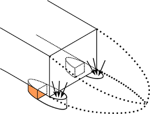
Figure 1. Experimental set-up.  $(a)$ Arrangement of the model and the raised floor, a detailed picture of the obstacles is depicted in $(b)$. $(c)$ Locations of pressure taps on the base, underside and behind the obstacles. Points indicate locations of mean pressure measurements and circles indicate locations of time-resolved pressure measurements. $(d)$ Particle image velocimetry (PIV) fields of view (FOVs) in the symmetry plane ( $y/H=0$, coloured in grey), cross-flow plane ( $x/H=0.03$, coloured in green) and half-ground-clearance plane ( $z/H=0.09$, coloured in red).
Unless otherwise stated, all the results presented are collected under a free-stream velocity  $U_{0} = 25$ m s $^{-1}$, corresponding to a height-based Reynolds number ${Re}_{H}=U_{0}H/v= 4.8 \times 10^{5}$, where $v$ is the kinematic viscosity of the air at operating temperature. For some representative test cases, $U_{0} = 20$ and 30 m s $^{-1}$ ( ${Re}_{H}= 3.8$ and $5.8 \times 10^{5}$) are also utilized to check the Reynolds number sensitivity. The origin $O$ of the coordinate system $(x,y,z)$ (shown in figure 1 $a$ behind the body) is located at the intersection point of the floor, the rear surface (the base) and the symmetry plane of the body, with $x$,
$x$,  $y$ and $z$ defined, respectively, along the streamwise, spanwise and floor-normal directions. Under this system, the velocity vector is decomposed into $\boldsymbol {u}=(u_{x},u_{y},u_{z})$. Unless otherwise stated, all physical quantities are normalized by any appropriate combination of the model height $H$, the free-stream velocity $U_{0}$ and the air density $\rho$ during the measurements. The Reynolds decomposition is employed to decompose a quantity $\mathcal {X}$ into $\mathcal {X}=\bar {\mathcal {X}}+\mathcal {X}'$, where $\bar {\mathcal {X}}$ and $\mathcal {X}'$, respectively, denote its time averaged and fluctuation components.
2.2. Underflow perturbations
In order to perturb the main wake as well as its drag, a similar approach to Wang (Reference Wang2019) is used with a pair of obstacles placed upstream of the base of the body, between the underside of the body and the floor (see figure 1 $a{,}b$). The two-dimensional (2-D) obstacles have a half-elliptic cross-section, whose length is 1.5 times the width $d$. This shape is chosen to minimize the influence of unwanted changes in the separation point on the interactions between the obstacles and the main wake. Several obstacle shapes were tested during preliminary measurements using a different square-back bluff body. It was shown that the drag of the body perturbed by obstacles with inertial separation is insensitive to the Reynolds number.
The widths of the obstacles are  $d/H = \{0.12, 0.16, 0.19, 0.22, 0.26\}$ and the height is $h/H=0.17$. The median width $d/H=0.19$ is the same as the width of the wheels used for example in Varney (Reference Varney2020) and Pavia et al. (Reference Pavia, Passmore, Varney and Hodgson2020). Therefore, the configuration using the $d/H=0.19$ obstacle pair is taken as the reference configuration and is subjected to substantial measurements. Between each obstacle and the body, a gap of 1.5 mm exists and is carefully filled with high-density foam to reduce the complexity of the flow and to focus on the interactions between the obstacles and the main wake. This disables the measurements of the aerodynamic force acting on the model. However, the main focus of the present work is the modifications in the main wake and therefore the base pressure is sufficient for quantifying the main effects of the obstacles.
The obstacle pair is always placed symmetric to the symmetry plane of the model, with its rear surface parallel to the base of the body and its left-hand/right-hand side tangents to the left-hand/right-hand side of the body. The degree of freedom of the pair in the streamwise direction is fixed by the obstacle-to-base distance  $l$, which is defined as the streamwise distance from the base of the obstacles to the base of the body. The parameter $l$ for all the $d/H$ configurations ranges from 0 $d$ (flush-mounted to the base) to 5 $d$.
$d$.
2.3. Pressure measurements
Two different pressure measurement systems are used to perform surface pressure measurements. The first one used for time averaged and long time scale measurements includes two 64-channel ESP-DTC pressure scanners linked to 1 mm diameter pressure taps located around the model by 78 cm long vinyl tubes. In total 128 taps are used but only the data from 25 taps on the base and 21 taps on the underside (see figure 1 $c$) are used in the present work. The taps on the base and on the underside are connected, respectively, to the two scanners with ranges of ${\pm }1$ and ${\pm }2.5$ kPa. The accuracy of the two scanners lies, respectively, below ${\pm }1.5$ and ${\pm }3.75$ Pa. Acquisitions from the scanners are conducted at a sampling rate of 100 Hz. For the reference configuration $d_{ref}/H=0.19$ with specific obstacle-to-base distances $l/d=\{0, 1.45,2.73, 4.91\}$, two 5.4 m-long tubes are arranged along the floor in order to obtain the mean base pressure of the obstacles. The pressure taps for this measurement are located at the centre of the base of the obstacles (see figure 1 $c$) and the tubes are connected to two differential pressure sensors located outside the test section (NovaSensor NPH802.50H). The sensors have a range of ${\pm }2.5$ kPa and an accuracy of ${\pm }5$ Pa.
The second system dedicated to time-resolved measurements contains four differential pressure sensors (SensorTechnics HCLA 02X5DB) connected to the pressure taps located on the base and the underside using 64 cm tubes. The tubing leads to a cutoff frequency of 150 Hz which is sufficient for resolving the presented time scales, therefore no frequency response calibration is applied. A sampling frequency of 2000 Hz is used for this system with an accuracy of  ${\pm }0.7$ Pa.
The pressure coefficient  $C_{p}$ is used to express the pressure measurements, and is defined as
 \begin{equation} C_{p}=\frac{p-p_{0}}{0.5 \rho U_{0}^{2}}, \end{equation}
where the reference static pressure  $p_{0}$ is obtained at $x/H=-1.6$ from a Pitot tube installed at the ceiling of the test section. For all the cases gathered, the duration of the pressure measurements is 300 s. For the unperturbed case presenting lateral bimodal behaviour on a long time scale of the order of $O(10^{3}H/U_{0})$ (Grandemange et al. Reference Grandemange, Gohlke and Cadot2013b), this measurement duration is not sufficient to obtain complete statistical convergence. Nevertheless, this time window is chosen as a compromise between a reasonable duration of the experimental campaign and a satisfactory convergence of the mean base pressure. For several mean base pressure values of the unperturbed case obtained from all measurement days (the campaign spans several weeks), the standard deviation of the mean base pressure values is below 2 % their average value. In order to further reduce the error due to the daily drift of the pressure measurement, the obtained base pressure values of the perturbed cases are expressed relative to the value of the unperturbed case of the same measurement day.
The pressure drag from the base is quantified by the base drag coefficient,
 \begin{equation} C_{B}={-}\frac{1}{25} \sum_{i=1}^{25} C_{p}(y_{i},z_{i},t), \end{equation}
where  $i$ represents the number of the 25 pressure taps on the base connected to the pressure scanner. The asymmetry of the main wake is characterized by the position of the base centre of pressure (CoP) $(y_{b},z_{b})$ relative to the centre of the base. The two components of the CoP are calculated by
 \begin{equation} y_{b}=\frac{{\sum}_{i=1}^{25} y_{i} C_{p}(y_{i},z_{i},t)}{H{\sum}_{i=1}^{25} C_{p}(y_{i},z_{i},t)}, z_{b}=\frac{{\sum}_{i=1}^{25} (z_{i}-G-H/2) C_{p}(y_{i},z_{i},t)}{H{\sum}_{i=1}^{25} C_{p}(y_{i},z_{i},t)}. \end{equation}
 Following Bonnavion & Cadot (Reference Bonnavion and Cadot2018), the pressure data used for calculating the CoP is low-pass filtered at 2 Hz ( $St_{H}=0.02$) through a moving average using a time window of 0.5 s in order to focus on the long-time dynamics of the main wake. In the same fashion as Varney (Reference Varney2020), the mean horizontal component of the base CoP $\overline {y_{b}}$ is used to achieved the zero yaw condition based on a pressure measurement of 10 minutes (i.e. $5 \times 10^{4}$ convective time units $H/U_{0}$). The turntable as shown in figure 1 $(a)$ is used to yaw the unperturbed body with an increment of $0.1^{\circ }$. The mechanical yaw angle with the minimum $|\overline {y_{b}}|$ is found to be $0.1^{\circ }$ and is chosen as the zero yaw condition.
For detailed investigation of the pressure measurements, we define  $\langle C_{p} \rangle$ as the spatial averaged pressure coefficient from the left-hand $L$ and right-hand $R$ side of the body in order to reduce the influence of any residual asymmetry of the main wake:
 \begin{equation} \langle {C_{p}} \rangle=\tfrac{1}{2}(C_{p}(y_{i},z_{i},t)+C_{p}({-}y_{i},z_{i},t)). \end{equation}
 The pressure taps used extensively in the investigation are numbered as  $n\in [1-6]_{L,R}$ as shown in figure 1 $(c)$.
2.4. Aerodynamic force measurements
A six-component aerodynamic balance (9129AA Kistler piezoelectric sensors and 5080A charge amplifier) connected to the model is used to quantify the unperturbed case. Measurements are performed at a sample rate of 200 Hz with a total accuracy below 0.6 % of the full range, representing 1 % in the mean drag force  $\overline {F_{x}}$ and 4 % in the mean lift force $\overline {F_{z}}$. The force coefficients are defined as
 \begin{equation} C_{i}=\frac{F_{i}}{0.5 \rho U_{0}^{2}HW}, \quad i \in \{x,y,z\}. \end{equation}
The force measurements are always performed simultaneously with the pressure measurements with the same sampling duration. Therefore, the same conclusion regarding the statistical convergence is achieved.
2.5. Velocity measurements
The velocity fields in the near wake are measured by a particle image velocimetry (PIV) system. The system consists of a Quantel EverGreen  $2 \times 200\,{\rm mJ}$ laser and two LaVision Imager LX 16 Mpx cameras. The seeding of the flow is introduced downstream of the raised floor and recirculates through the tunnel in a closed circuit. Particles with a diameter of $1\, \mathrm {\mu }{\rm m}$ are generated by atomization of mineral oil. Three 2-D fields of view (FOVs) are considered as depicted in figure 1 $(d)$. The first one located in the symmetry plane of the body ( $y/H=0$) is of 2-D two-component (2D2C) set-up, obtaining the streamwise $u_{x}$ and vertical $u_{z}$ velocity components. The other two FOVs are, respectively, located in a cross-flow plane in proximity to the base of the body ( $x/H=0.03$) and a plane at half the height of the ground clearance ( $z/H=0.09$). These two FOVs are of stereoscopic (2-D three-component (2D3C)) set-up, capturing three velocity components. The notation and the space spanning of the PIV FOVs are given in table 1.
Table 1. Details of PIV FOVs.

For representative cases, 1200 pairs of images are captured from each FOV at a sample rate of 4 Hz, which is satisfactory for statistical convergence of first- and second-order statistics. Image pairs are processed using DaVis 10.1 with a final interrogation window of  $32 \times 32$ pixels for the 2D2C FOV and $16 \times 16$ pixels for the 2D3C FOVs. All the processing is performed with an overlap of 50 %. The resulting vector spacing for each measurement plane is summarized in table 1. The maximum uncertainty on the instantaneous velocity fields from different FOVs considering an absolute displacement error of 0.1 pixels is estimated to be less than $0.01U_{0}$.
3. Unperturbed flow
Before perturbing the underflow using the obstacle pair, we briefly characterize the unperturbed case. To this end, the wake flow is presented in figure 2.

Figure 2. Unperturbed flow.  $(a)$ Mean velocity components ( $\overline {u_{x}}$ and $\overline {u_{z}}$) and turbulent kinetic energy ( $k=(\overline {u_{x}'u_{x}'}+\overline {u_{z}'u_{z}'})/2$) in the symmetry ( $y/H=0$) and cross-flow ( $x/H=0.03$) planes. $(b)$ Conditional averaging of the base pressure distribution based on the joint probability density function (p.d.f.) of the base CoP position $(y_{b},z_{b})$ (no low-pass filter is applied), the horizontal blue dotted line indicates $\overline {z_{b}}$ and the probability is normalized by its highest value. Flow topology of each wake state is given by $\overline {u_{y}}$ in the cross-flow plane for each flow state.
The time-averaged streamwise  $\overline {u_{x}}$ and vertical $\overline {u_{z}}$ velocity components in the symmetry ( $y/H=0$) and cross-flow ( $x/H=0.03$) planes describe a wake with vanishing vertical asymmetry. The global topology is qualitatively similar to the wake captured in Pavia et al. (Reference Pavia, Passmore, Varney and Hodgson2020) using also a Windsor geometry but with a shorter length of the geometry. As detailed in Haffner et al. (Reference Haffner, Borée, Spohn and Castelain2020), this type of wake is of weak interaction between its top and bottom shear layers. Depicting the turbulent kinetic energy $k=(\overline {u_{x}'u_{x}'}+\overline {u_{z}'u_{z}'})/2$, almost balanced turbulent levels are noticed between the top and bottom shear layers. Therefore, with the underflow perturbed, a change in the vertical wake balance may lead to a drag increase as shown in Haffner et al. (Reference Haffner, Castelain, Borée and Spohn2021).
In the horizontal direction, the wake exhibits the well known long-time random switching motion (Grandemange et al. Reference Grandemange, Gohlke and Cadot2013b) with two equiprobable states as presented in figure 2 $(b)$. The two states are given by the joint probability density function (p.d.f.) of the two components of the base CoP position. Further conditional averaging based on the sign of the horizontal component of the base CoP position $y_{b}$ gives the flow topology of the two wake states, which is dominated by a large recirculating flow located at the left-hand and right-hand sides, respectively.
We summarize the time-averaged global quantities in table 2. The quantities include the forces acting on the body, the length of the recirculating flow and the mean values of the CoP. The recirculation length is defined as the maximum downstream location of  $\overline {u_{x}}\leq 0$, as follows:
 \begin{equation} L_{r}=\textit{max}(x/H)_{\overline{u_{x}}(x/H)\leq 0}. \end{equation}
Table 2. Mean aerodynamic coefficients for the unperturbed case: forces (drag, lift and base drag coefficients), recirculation length, mean vertical position and mean modulus of the base CoP.

The modulus of the base CoP position  $r_{b}$ is used to quantify the strength of the static symmetry-breaking mode, which is calculated by including the elliptic model proposed in Bonnavion & Cadot (Reference Bonnavion and Cadot2018):
 \begin{equation} (r_{b})^{2}=\left(\frac{y_{b}}{W/H}\right)^{2}+(z_{b})^{2}. \end{equation}
 The drag and lift coefficients are in good accordance with the measurements by Howell & Le Good (Reference Howell and Le Good2005) using a Windsor geometry with the same ground clearance, who obtained  $\overline {C_{x}}=0.232$ and $\overline {C_{z}}=-0.122$. The slight difference could be attributed to the differences in the model geometry (different lengths) as well as the support method. Favre & Efraimsson (Reference Favre and Efraimsson2011) also obtained a series of $\overline {C_{x}}$ using detached eddy simulations, which ranged from 0.222 to 0.229. The base drag $\overline {C_{B}}$ is also in good accordance with previous studies based both on Windsor and Ahmed geometries with a vertical balanced wake, for example in Grandemange et al. (Reference Grandemange, Gohlke and Cadot2013b) and Varney (Reference Varney2020). Under different free-stream velocities, the base drag shows no obvious change after $Re_{H} \geq 4.8 \times 10^{5}$.
4. Global effects of perturbations: base drag sensitivity and pressure fields
4.1. Base drag sensitivity
We present first the base drag variation  $\Delta \overline {C_{B}}=\overline {C_{B}}-\overline {C_{B0}}$ with varying obstacle-to-base distance $l/d$ for the reference configuration $d_{ref}/H=0.19$ in figure 3. Moving the obstacle pair from the most upstream position ( $max\{l\}/d$) towards the base, the configuration presents first a plateau with a slight increase in base drag, followed by a drag-sensitive regime with a rapid base drag increase until the flush-mounted position is reached. In the drag-sensitive regime, the maximum base drag increase is $\Delta \overline {C_{B}}/\overline {C_{B0}}\approx 18\,\%$. This important drag increase indicates a great sensitivity of drag to the obstacle-to-base distance. Therefore, the present work aims at educing the interaction mechanisms between the wakes of the obstacles and the main wake in the drag-sensitive regime. We also notice that the slope of the monotonous base drag increase experiences a sudden change at $l/d \approx 1.5$. A criterion based on the mean and fluctuating properties in the wake of the obstacles, detailed later in § 4.2, will show that we observe two regimes which are characterized by different interaction mechanisms between the wakes of the obstacles and the main body. We name these two regimes as regime I and II. The Reynolds number sensitivity is also checked for some cases as shown by different colours, we observe no obvious dependence of $\Delta \overline {C_{B}}$ on the free-stream velocity (below 0.5 % of $\overline {C_{B0}}$).

Figure 3. Base drag of the body  $\Delta \overline {C_{B}}=\overline {C_{B}}-\overline {C_{B0}}$ as a function of the obstacle-to-base distance $l/d$ for the reference configuration $d_{ref}/H=0.19$.
Before analysing detailed local measurements, integral measurements can be very helpful in exploring scaling properties. Figure 4 $(a{,}b)$ show the evolution of $\Delta \overline {C_{B}}$ for all the $d/H$ configurations. Using the same criterion as the reference configuration which will be shown later in § 4.2, regime I and the plateau are coloured in red and regime II is coloured in blue. Few cases present transition between the two regimes as indicated by the green colour and are detailed also in § 4.2. In these two figures, the obstacle-to-base distance $l$ is scaled, respectively, with the height of the body $H$ and the width of the obstacles $d$. It is clearly shown that $l/d$ is the correct scaling as the distance to the base is concerned. For all the available cases, the $l/d$ ranges for the plateau, regime I and regime II are $l/d>2.5$, $2.5>l/d\geq 1.56$ and $1.45\geq l/d\geq 0$, respectively.

Figure 4. Impact of the position  $l$ and width $d$ of the obstacles on the base drag of the body; darker colour indicates wider obstacle. The base drag is scaled by $l/H$ ( $H$ is the height of the model) in $(a)$ and $l/d$ in $(b)$. See § 4.2 for the meaning of the colours.
Moreover, the sensitivity of  $\Delta \overline {C_{B}}$ to $l/d$ also depends on the obstacle width $d/H$ as shown in figure 4 $(b)$. Concentrating first on regime I, with decreasing $l/d$, the base drag increases from the end of the plateau. Along the plateau the obstacles are expected to induce perturbations of the underflow that may alter the near-wake balance as shown by Barros et al. (Reference Barros, Borée, Cadot, Spohn and Noack2017) and used by Haffner et al. (Reference Haffner, Castelain, Borée and Spohn2021). In our situation, a base drag increase of ${\sim }5\,\%$ is observed in the plateau for all the configurations from the unperturbed case. In order to focus only on the base drag sensitivity in regime I and remove the drag increase of $\sim 5\,\%$, we define a variant of the base drag variation $\Delta \overline {C_{B}}^{I}=\overline {C_{B}}(l/d)-\overline {C_{B}}(l/d=2.5)$. More precisely, the base drag values of the cases with $l/d$ values closest to $l/d=2.5$ are approximately used as $\overline {C_{B}}(l/d=2.5)$. Figure 5 $(a)$ then shows a clear scaling property of the base pressure variation in regime I,
 \begin{equation} \Delta \overline{C_{B}}^{I}=(d/d_{ref})^{2}\Delta \overline{C_{B}}_{ref}^{I}, \end{equation}
where  $\overline {C_{B}}_{ref}^{I}$ denotes the base drag evolution of the reference configuration. Using quadratic fitting, the base drag evolution in regime I can be approximated for all the $d/H$ configurations: $\Delta \overline {C_{B}}^{I} = 0.2(d/H)^{2}(2.5-l/d)^{2}$. On the other hand in regime II (figure 5 $b$), the main trend observed is a linear shift of $\Delta \overline {C_{B}}$ proportional to the width of the obstacles $d$, i.e.
 \begin{equation} \Delta \overline{C_{B}} = (d/d_{ref}) \Delta \overline{C_{B}}_{ref}. \end{equation}
Figure 5. Scalings of the base drag evolution in regime I  $(a)$ and in regime II $(b)$.
Similarly to regime I, a quadratic fitting gives  $\Delta \overline {C_{B}} = 0.03(d/H)((l/d)^{2}-3.3l/d+6.5)$. The physical arguments for these specific scaling properties will be detailed in § 6 in order to help building a physical model of the phenomenon.
4.2. Pressure fields
In order to better understand the base drag increase under the perturbation of the obstacles, we now analyse the mean pressure fields over the body and in the wake of the obstacles, starting by the mean base pressure distribution of the reference configuration in figure 6 $(a)$. On the right-hand side of the base, the distribution of pressure difference $\Delta \langle \overline {C_{p}} \rangle$ with respect to the unperturbed case is also presented for comparison. From case $l/d=4.91$ to $l/d=1.64$, the transition from the plateau to regime I is described. On the other hand, from $l/d=1.45$ to $l/d=0$, regime II is visualized. In the plateau, the base pressure decrease of ${\sim }5\,\%$ from the unperturbed case is located at the bottom half of the base with a slight pressure recovery at the top half. This observation of top/bottom symmetry breaking was also captured by Barros et al. (Reference Barros, Borée, Cadot, Spohn and Noack2017) using similar underflow perturbations situated far from the base ( $l/d>4$). In regime I, we observe a further pressure decrease at the bottom half of the base with now also a slight decrease at the top half. The pressure decrease is not homogeneous laterally but rather located near the obstacles.

Figure 6.  $(a)$ Evolution of the base pressure distribution with the obstacle-to-base distance $l/d$ for the reference configuration $d_{ref}/H=0.19$, the mean values and the differences with respect to the unperturbed case are, respectively, presented at the left-hand and right-hand sides of the base. $(b)$ Evolution of the mean vertical position of the base CoP $\overline {z_{b}}$ with $l/d$. $(c)$ Comparison between the evolution of $\langle \overline {C_{p5}} \rangle$ and $\langle \overline {C_{p6}} \rangle$ for the reference configuration $d_{ref}/H=0.19$.
In regime II, the base pressure is importantly modified and the modification is mainly located at the bottom half of the base and horizontally near the obstacle pair. This observation indicates that in regime II the interactions between the main wake and the wakes of the obstacles greatly modify the structure of the main wake. This is better illustrated in figure 6 $(b)$ by the mean vertical position of the base CoP $\overline {z_{b}}$. In the plateau and regime I no obvious modification in $\overline {z_{b}}$ is witnessed. However, in regime II, $\overline {z_{b}}$ decreases continuously with decreasing $l/d$.
We now consider the pressure distribution in the vicinity of the obstacles. In figure 6 $(c)$ a comparison is presented between the evolution of $\langle \overline {C_{p5}} \rangle$ and $\langle \overline {C_{p6}} \rangle$ for the reference configuration. As shown in the sketch in figure 6, sensors $5_{L}$ and $6_{L}$ ( $5_{R}$ and $6_{R}$) are located in the symmetry plane of the left-hand (right-hand) reference obstacle. They are positioned on both sides of the bottom trailing edge of the body, which are the key locations for the problem considered here. In the plateau, $\langle \overline {C_{p5}} \rangle$ is slightly higher than $\langle \overline {C_{p6}} \rangle$. This is expected for a mean curved streamline after separation, inducing a lower pressure inside the recirculating bubble due to centrifugal effect (Bradshaw Reference Bradshaw1973). However, in both regime I and II, $\langle \overline {C_{p5}} \rangle$ is lower than $\langle \overline {C_{p6}} \rangle$. With decreasing $l/d$, the pressure difference $\langle \overline {C_{p6}} \rangle -\langle \overline {C_{p5}} \rangle$ increases strongly in regime I. On the contrary, in regime II, $\langle \overline {C_{p6}} \rangle -\langle \overline {C_{p5}} \rangle$ decreases with decreasing $l/d$, which gives a possible explanation for the sudden change in the slope of the base drag evolution between regime I and II.
The influence of the obstacles on the main wake as presented using  $\langle \overline {C_{p5}} \rangle$ changes rapidly in the drag-sensitive regimes. Therefore, we turn to the perspective of the obstacles to understand the evolution of $\langle \overline {C_{p5}} \rangle$. To this aim, an obstacle-fixed reference frame is defined and is shown in figure 7 $(a)$. The origin $O_{d}$ lies at the intersection point of the floor, the base of the left-hand obstacle and the symmetry plane of the left-hand obstacle. In this way, as shown in figure 7 $(b)$, the pressure taps indicated by red symbols act like a streamwise pressure rake. We choose four $l/d$ cases of the reference configuration as an example in figure 7 $(b)$. At each $l/d$ location, the streamwise pressure development in the wake of the obstacles can be at best characterized by five pressure taps except that for small $l/d$, some of the taps with $x_{d}/d<0$ are covered by the obstacles. The $\langle \overline {C_{pn}} \rangle$ values obtained from the available pressure taps, therefore, can be gathered onto a single plot in figure 7 $(c)$. This allows a comparison of the streamwise pressure development behind the obstacles between different $l/d$ cases. We proceed further in figure 8 $(a)$ by presenting the evolution of $\langle \overline {C_{pn}} \rangle$ with $x_{d}/d$ for all the $d/H$ configurations. Typical base pressure coefficients $\overline {C_{pb}}$ from previous studies are also presented for comparison.

Figure 7.  $(a)$ Definition of an obstacle-fixed coordinate system. $(b)$ The relative position of the obstacle and the pressure taps for cases $l/d=4.90$, $2.73$, $1.45$ and $0$ of the reference configuration $d_{ref}/H=0.19$. $(c)$ Evolution of the time- and space-averaged pressure coefficients $\langle \overline {C_{pn}} \rangle$ obtained from the pressure taps used ( $n \in [1,2,3,4,5]$) as a function of the streamwise distance from the base of the obstacles $x_{d}$, only the cases in $(b)$ are shown with colours related to the $l/d$ values.

Figure 8. Pressure evolution in the wake of the obstacles: evolution of  $\langle \overline {C_{pn}} \rangle$ ( $n \in [1,2,3,4,5]$) as a function of $x_{d}$ for all the cases $(a)$ and for the cases around the boundary of regimes $(b)$; different colours indicate different flow regimes.
In regime I and the plateau, the streamwise pressure developments in the wake of the obstacles superimpose on a same curve (coloured red). Near the obstacle base, the pressure  $\langle \overline {C_{pn}} \rangle \sim -0.5$ is of the same level as the base pressure values measured by Bearman (Reference Bearman1967) and Park et al. (Reference Park, Lee, Jeon, Hahn, Kim, Kim, Choi and Choi2006) using 2-D bluff bodies with similar cross-section shapes as the obstacle. Downstream of the obstacle base, the strong longitudinal pressure gradient along $1< x_{d}/d<2.5$ towards $\langle \overline {C_{pn}} \rangle \sim -0.2$ indicates closure of the obstacle wake bubble. For a reference 2-D mean wake, the increase in mean static pressure can be understood by writing the streamwise momentum balance along the centreline:
 \begin{equation} -\frac{1}{2} \frac{\partial \overline{C_{p}}}{\partial x}= \overline{u_{x}} \frac{\partial \overline{u_{x}}}{\partial x} + \frac{\partial \overline{u_{x}'u_{x}'}}{\partial x} + \frac{\partial \overline{u_{x}'u_{y}'}}{\partial y}. \end{equation}
 From the reference studies on 2-D bluff bodies (Balachandar, Mittal & Najjar Reference Balachandar, Mittal and Najjar1997; Konstantinidis, Balabani & Yianneskis Reference Konstantinidis, Balabani and Yianneskis2005; Parkin, Thompson & Sheridan Reference Parkin, Thompson and Sheridan2014), it is possible to find out that the term  $\partial \overline {u_{x}'u_{y}'}/ \partial y$ dominates the region of strong longitudinal increase of mean pressure. Moreover, in this region, the Reynolds shear stress $\overline {u_{x}'u_{y}'}$ is mainly the signature of the Kármán vortex shedding.
At a specific  $l/d$ position, the pressure value at the bottom trailing edge of the body downstream of the obstacles is equal to the $\langle \overline {C_{pn}} \rangle$ value at $x_{d}/d=l/d$. In regime I ( $1.56 \leq l/d<2.5$), the trailing edge experiences a sharp pressure decrease with decreasing $l/d$. This was shown before in figure 6 $(c)$ by the evolution of $\langle \overline {C_{p5}} \rangle$ with $l/d$. The transition from regime I to regime II is pictured in figure 8 $(b)$ by presenting only the cases near the boundary of the regimes. It is clear that despite the small $l/d$ change, the pressure in the obstacle wake is completely altered.
Regime II (coloured blue in figure 8 $a$) presents a higher pressure near the obstacle base ( $x_{d}/d<1$). A strong coupling between the main wake and the wakes of the obstacles is expected in this regime. The pressure recovery near the obstacle base from regime I to regime II is approximately 34 %. It is interesting to note that a similar trend of pressure recovery is obtained in the wakes of 2-D bluff bodies when flow control techniques are applied, with the natural Kármán vortex shedding in these wakes attenuated by 3-D perturbations using tab devices (Park et al. Reference Park, Lee, Jeon, Hahn, Kim, Kim, Choi and Choi2006) or by splitter plate (Bearman Reference Bearman1965).
The different streamwise pressure developments in different regimes efficiently distinguish the cases belonging to regime I and II. At different  $l/d$ positions in the same regime, the wakes of the obstacles keep their mean properties. Hence, the obstacles are decisive for the global evolution of the flow. Apart from the two regimes, some cases present intermediate pressure levels near the base of the obstacles which lie between the two regimes and are coloured green. It is important to note here that the cases are carefully checked and no obvious difference is found in the pressure between taps located on two sides. This prevents the situation that the two obstacles are subjected, respectively, to different regimes.
We now investigate the pressure dynamics in the wake of the obstacles. The focus is put on the Kármán vortex shedding observed in 2-D wakes. The existence of the vortex shedding in such a scenario is captured by Zhang, Zhou & To (Reference Zhang, Zhou and To2015) and Wang et al. (Reference Wang, Zhou, Pin and Chan2013). In their works two different  $St_{d}$, respectively behind the front and rear cylindrical struts used for model supporting, are reported and are interpreted as the signatures of the vortex shedding ( $d$ denotes the diameter of the struts). By carefully examining the spectral content of the unsteady pressure sensors, the coherent dynamics of the obstacle wake are captured by taps $5_{L}$ and $5_{R}$ located downstream of the obstacle pair. The premultiplied spectra obtained from $5_{L}$ and $5_{R}$ are averaged and the result is shown in figure 9 $(a)$. Only the two cases near the dividing point, $l/d=1.45$ (regime II) and $1.64$ (regime I), are pictured. A clear distinction is noticed between the cases, where an important peak is noticed for the case $l/d=1.64$ (regime I). This peak occurs at $St_{d}=0.26$ which is in good agreement with the studies based on D-shaped cylinders (Bearman Reference Bearman1965, Reference Bearman1967; Park et al. Reference Park, Lee, Jeon, Hahn, Kim, Kim, Choi and Choi2006). In these studies, the authors interpret the peak frequency as the vortex shedding frequency. On the other hand, in regime II the pressure fluctuation is much weaker and the peak at $St_{d}=0.26$ is barely discernible, implying suppression of the periodic motion.

Figure 9. For the reference configuration  $d_{ref}/H=0.19$: $(a)$ premutiplied spectra of the pressure data obtained from taps $n=5$ for cases $l/d=1.45$ and $l/d=1.64$. $(b)$ Evolution of the premultiplied spectrum of the pressure signal $C_{p5}$ with $l/d$. $(c)$ Spectral coherence between pressure signals $C_{p5}$ and $C_{p6}$.
For the reference configuration, the evolution with  $l/d$ of the premultiplied spectrum of the pressure signals from the taps numbered 5 is presented in figure 9 $(b)$. In regime I, the continuous decrease in $\langle \overline {C_{p5}} \rangle$ with decreasing $l/d$ is accompanied by an increase in the energy of the peak at $St_{d}=0.26$ thus the coherent dynamics have growing effects on the main wake. On the other hand in regime II, although the peak at $St_{d}=0.26$ is not observable, relatively lower energy is found at very low frequency. This suggests that through the expected wake coupling as envisioned before, the wakes of the obstacles are influenced by the low-frequency dynamics of the main wake.
We present further the spectral coherence  $Coh_{p_{5}p_{6}}$ of the unsteady pressure sensors named by $5_{L,R}$ and $6_{L,R}$ as depicted in figure 7, which is calculated via
 \begin{equation} Coh_{p_{5}p_{6}}=0.5 \sum_{i=L,R}^{i}\left(\frac{|S_{p_{5i}p_{6i}}|^{2}}{S_{p_{5i}p_{5i}}S_{p_{6i}p_{6i}}}\right), \end{equation}
where  $S_{p_{5i}p_{5i}}$ and $S_{p_{6i}p_{6i}}$ are the power spectral densities of the pressure coefficients $C_{p5i}$ and $C_{p6i}$, respectively, and $S_{p_{5i}p_{6i}}$ is the cross power spectral density of the pressure coefficients $C_{p5i}$ and $C_{p6i}$ ( $i$ denotes $L$ or $R$). The evolution of $Coh_{p_{5}p_{6}}$ with $l/d$ is presented in figure 9 $(c)$. It is shown that in regime I the base pressure is strongly coupled with the coherent dynamics at $St_{d}=0.26$. We also observe a strong coherence at low frequency in the plateau and regime II. Apart from the bistable dynamics, this frequency range of $0.05< St_{H}<0.21$ (based on the height of the body) also contains several coherent dynamics of the main wake, for example the low-frequency pumping motion of the recirculation region observed by Volpe, Devinant & Kourta (Reference Volpe, Devinant and Kourta2015) and Dalla Longa, Evstafyeva & Morgans (Reference Dalla Longa, Evstafyeva and Morgans2019). The lack of coherence in the low-frequency range in regime I suggests that the wake dynamics of the obstacles dominates the interactions between the obstacles and the main wake.
The coupling between the dynamics of the main wake and the wakes of the obstacles promotes an investigation on the low-frequency dynamics of the main wake, which could be helpful to better understand the interaction mechanisms. The sensitivity map of the CoP position  $y_{b}$ and $z_{b}$ to $l/d$ is presented in figure 10 $(a)$. For all the configurations ( $d/H=0.16$ and $0.22$ are not shown for clarity), the horizontal bistable dynamics is observed during the entire regime I and the plateau. In regime II, a gradual suppression of asymmetry in the horizontal direction with decreasing $l/d$ is observed. This suppression is accompanied by an increase in asymmetry in the vertical direction. For the $d/H=0.19$ and $0.26$ configurations with decreasing $l/d$, the vertical symmetry breaking in regime II rotates the two bistable states to a locked state with a permanent asymmetry in the vertical direction. Finally, the evolution of the static symmetry-breaking mode strength $\overline {r_{b}}$ with $l/d$ is shown in figure 10 $(b)$. The cases with a horizontal bimodal asymmetry and a locked vertical asymmetry are presented, respectively, at the left-hand and right-hand side. For the cases with a horizontal bimodal asymmetry, $\overline {r_{b}}$ decreases slightly with decreasing $l/d$ in regime I and the plateau. This decrease in $\overline {r_{b}}$ is strengthened in regime II, and maximally leads to a ${\sim }30\,\%$ reduction in the static mode from the cases of maximum $l/d$. It is interesting to note here that the cases with a permanent asymmetry along the minor axis of the base do not follow the same trend.

Figure 10.  $(a)$ Sensitivity maps of the horizontal and vertical CoP position $y_{b}$ and $z_{b}$ to $l/d$ for the configurations $d/H=[0.12,0.19,0.26]$, the p.d.f. of each $l/d$ case is normalized by its most probable value. $(b)$ Evolution of the mean modulus of base CoP position $\overline {r_{b}}$ with $l/d$, the cases with locked wake asymmetry are presented separately. $(c)$ Sensitivity maps of the pressure signal $C_{p5L}$ to $l/d$ for the reference configuration $d_{ref}/H=0.19$, the p.d.f. of each $l/d$ case is normalized by its most probable value.
The low-frequency content in the plateau and regime II as discussed in figure 9 $(c)$ is further investigated by checking the time evolution of the pressure signal from tap $5_{L}$, it is found in figure 10 $(c)$ that in the plateau and regime II, the time evolution of the pressure presents two preferred values. However, in regime I, we observe only one peak in the p.d.f. of $C_{p5L}$, which is consistent with the investigation using the spectral coherence in figure 9 $(c)$.
5. Global and local wake modifications
The flow mechanisms resulting in the base drag sensitivity in different regimes are investigated in this section. A global description of the main wake is presented first, which is followed by a detailed analysis of the wake of the obstacles. Most of the investigations in this section are based on the reference configuration since other configurations provide the same conclusions.
5.1. Evolution of the near wake of the body
We now describe the time-averaged main wake for the reference configuration in figure 11 $(a)$, which is the origin of the low-pressure footprint over the base. From the plateau to regime I, the recirculating bubble is shortened by 2.5 %, and the base drag increases by 3.7 %. In regime II, the base drag increase is also accompanied by the decrease in bubble length. We observe a sudden increase in $L_{r}$ of 2 % from $l/d=1.64$ to $l/d=1.45$. The whole evolution of the recirculation length $\Delta L_{r}= L_{r}-L_{r0}$ with $l/d$ is further shown in figure 11 $(b)$ and the sudden increase in $L_{r}$ is again confirmed. This indicates that the interactions between the main wake and the wakes of the obstacles in the two regimes are totally different.

Figure 11. Evolution of the main wake topology with  $l/d$ for the reference configuration $d_{ref}/H=0.19$. $(a)$ Streamlines in the symmetry plane ( $y/H=0$) for cases of the plateau ( $l/d=4.91$), regime I ( $l/d=1.64$) and regime II ( $l/d=1.45$ and $0$). The dashed curve represents the separatrix of the $l/d=4.91$ case. $(b)$ Evolution of the recirculation length $L_{r}$ with $l/d$. $(c)$ Comparison of the recirculation strength $\mathcal {R}$ for the cases presented in $(a)$.
Apart from the mean velocity fields discussed, where the flow curvature importantly influences the base drag, the Reynolds stresses also play an important role in the base drag as interpreted through the streamwise momentum balance proposed by Balachandar et al. (Reference Balachandar, Mittal and Najjar1997) for 2-D wakes. This momentum balance was also used in 3-D situations, for example in Grandemange et al. (Reference Grandemange, Gohlke and Cadot2013a) and Liu et al. (Reference Liu, Zhang, Zhang and Zhou2021), to emphasize the importance of the mean transport of the fluctuating momentum by turbulent velocity fluctuations. One of the consequences of the Reynolds stresses in the mean velocity fields is the changes in the intensity of the recirculating flow, since they represent the small-scale entrainment and large-scale engulfment inside the recirculation region. The intensity of the recirculating flow is measured by a quantity  $\mathcal {R}$, which is defined as
 \begin{equation} \mathcal{R}(x)=\int_{{\overline{u_{x}}\leq 0}}|\overline{u_{xz}}(x,z)|\,{\rm d}z, \end{equation}
where  $|\overline {u_{xz}}|=\sqrt {\overline {u_{x}}^{2}+\overline {u_{z}}^{2}}$. This quantity is displayed in figure 11 $(c)$. It is shown that the obstacle pair leads to an overall enhancement of the recirculating motion from the unperturbed case. For the case with the highest drag increase ( $l/d=0$), the maximum of the recirculation strength $\mathcal {R}$ increases substantially by ${\sim }50\,\%$ from the unperturbed case. With decreasing $l/d$, we observe that the drag and the recirculation strength increase continuously. This is not the case for the recirculation length as observed in figure 11. The recirculation length should therefore be used with particular caution when analysing complex wakes.
A detailed examination of the Reynolds stresses in the symmetry plane is presented in figure 12. Comparing these three selected cases, no obvious difference is noticed in the  $\overline {u_{x}'u_{x}'}$ and $\overline {u_{x}'u_{z}'}$ (not shown here for brevity) components. The $\overline {u_{z}'u_{z}'}$ component, on the other hand, shows more evident changes. From the plateau ( $l/d=4.91$) to regime I ( $l/d=1.64$), $\overline {u_{z}'u_{z}'}$ increases locally in the bottom shear layer and in the end of the mean wake bubble. However, from regime I ( $l/d=1.64$) to regime II ( $l/d=0$), the predominant increase is localized in the top shear layer. A quantitative comparison is achieved by integrating the absolute value of the stresses inside a rectangular region $\mathcal {S}$ limited by the body height as shown in figure 12 $(b)$. The reference case is also shown for comparison. It is clear that the obstacle pair globally enhances the turbulent fluctuations in the wake compared with the reference case, proved by the substantial increases in all components. For the perturbed cases, $|\overline {u_{x}'u_{x}'}|_{int_{\mathcal {S}}}$ and $|\overline {u_{x}'u_{z}'}|_{int_{\mathcal {S}}}$ have the same evolution, with no obvious change from the plateau to regime I and a slight increase from regime I to regime II. On the other hand, $|\overline {u_{z}'u_{z}'}|_{int_{\mathcal {S}}}$ increases substantially from case $l/d=4.91$ to $l/d=1.64$ followed by a slight increase from case $l/d=1.64$ to $l/d=0$.

Figure 12. Reynolds stresses in the symmetry plane  $y/H=0$ for the cases of the plateau ( $l/d=4.91$), regime I ( $l/d=1.64$) and regime II ( $l/d=0$). The width of the obstacles is $d_{ref}/H=0.19$. $(a)$ Normal stress $\overline {u_{x}'u_{x}'}$ and $\overline {u_{z}'u_{z}'}$. $(b)$ Streamwise profiles of the integrals of Reynolds stresses over region $\mathcal {S}$.
We present now a 3-D description of the main wake by gathering the velocity measurements in the three PIV planes. The velocity distributions are shown in figure 13 for three cases of the reference configuration in the plateau ( $l/d=4.91$), regime I ( $l/d=1.82$) and regime II ( $l/d=0$). Focusing first on the streamwise velocity $\overline {u_{x}}$ distributions (figure 13 $a$), no obvious difference between the cases is noticed in the main wake. However, as also observed by Wang (Reference Wang2019), the different sensitivities in different regimes are marked by the momentum deficit behind the obstacles, where in regime II ( $l/d=0$) the same velocity level as in the recirculation region of the main wake is observed in the cross-flow plane. This indicates that in regime II the wakes are merged. For these three cases, the velocity at the exit of the underbody in the centre region in-between the obstacles (see measurements in plane $x/H=0.03$) does not evolve from the unperturbed flow. More generally, only very minor modifications of this longitudinal underflow momentum between the obstacles are observed for varying $l/d$ and $d/H$. In addition to the wake merging, regime II also presents a strong downwash flux from the main wake to the wakes of the obstacles as depicted using the vertical velocity $\overline {u_{z}}$ in figure 13 $(b)$. Concomitantly, the downward motion in the bottom half of the main wake is enhanced. This downward flux is possibly the main reason for the enhancement of the recirculation strength and the modification in the vertical balance of the main wake. We show the strength of the cross-flow near the base of the body by defining a quantity $\mathcal {E}$, such that
 \begin{equation} \mathcal{E}(z)=\int_{\mathcal{B}}|\overline{u_{yz}}|(y,z)\,{{\rm d}y}, \end{equation}
where  $|\overline {u_{yz}}|=\sqrt {\overline {u_{y}}^{2}+\overline {u_{z}}^{2}}$ and the integral region is $\mathcal {B} = y/H \times z/H = [-W/2, W/2] \times [G, G+H]$ over the cross-flow plane. The boundary of $\mathcal {B}$ is the projection of the edges of the base to the present plane. The quantity is displayed in figure 13 $(c)$ for the selected cases as well as the unperturbed case. With the underflow perturbed at the most upstream position, the bottom part of the recirculating flow is enhanced. Entering into regime I, $\mathcal {E}$ is globally higher than in the plateau but is more balanced vertically. Arriving at the flush-mounted position, $\mathcal {E}$ increases and a stronger bottom recirculating flow is observed. All the observations are in accordance with the investigation based on the base pressure.

Figure 13. Mean velocity components,  $(a)$
$(a)$  $\overline {u_{x}}$ and $(b)$
$(b)$  $\overline {u_{z}}$, in the three PIV planes for the cases of the plateau ( $l/d=4.91$), regime I ( $l/d=1.82$) and regime II ( $l/d=0$). The width of the obstacles is $d_{ref}/H=0.19$. $(c)$ Comparison of the cross-flow strength $\mathcal {E}$, the space-averaged values are shown over the top axis. $(d)$ Turbulent kinetic energy $k$ distributions in the three PIV planes for the same cases as $(a{,}b)$.
By looking at the fluctuating velocity fields, we also observe a profound difference of the case in regime I, which is presented in figure 13 $(d)$ by the distributions of the turbulent kinetic energy $k$. A strong unsteady motion is detected in the wakes of the obstacles in regime I but not in regime II. This trend from the plateau to regime II is in accordance with the spectral information shown before in figure 9. All the differences between regimes are located near the obstacles and therefore the mean wake interactions are studied locally around the obstacles in the following section.
5.2. Obstacle wake characteristics in different regimes
In this section, we focus on the wake dynamics of the obstacles in different regimes following the obstacle-fixed coordinate system defined in figure 7. This helps us to understand the differences between different flow regimes observed in figure 13 near the obstacles. Unless otherwise stated, the obstacle considered in this section is the obstacle located at the left-hand side ( $y/H<0$) because the right-hand obstacle is only a mirror symmetry of the left-hand one in a time-averaged point of view.
Figure 14 presents the distributions of the mean streamwise velocity  $\overline {u_{x}}$ at $z/H=0.09$ (plane XY) and $x/H=0.03$ (plane YZ) downstream the obstacle. Meanwhile, under the obstacle-fixed reference frame, plane YZ moves downstream with $l/d$. The relative positions of plane YZ to plane XY are marked by the traverse dotted lines in figure 14 $(a{,}b)$. Starting from a case in the plateau, the left-hand two columns, case $l/d=2.72$ and $1.82$ characterize the evolution from the plateau to regime I. On the other hand, $l/d=1.45$, $0.73$ and $0$ describe the development of regime II.

Figure 14. Evolution of the mean streamwise velocity  $\overline {u_{x}}$ with the obstacle-to-base distance $l/d$ downstream the left-hand obstacle $d/H=0.19$ at $z/H=0.09$ $(a)$ and $x/H=0.03$ $(b)$, the $\overline {u_{x}}$ distributions along $y_{d}/d=0$ in $(b)$ are detailed in $(c)$. $(d)$ Evolution of the space-averaged mean vertical velocity $\langle \overline {u_{z}} \rangle$ with $l/d$ for the reference configuration, the line used for space averaging is indicated in $(b)$ (see text for details).
We focus first on the cases near the dividing point, case  $l/d=1.82$ and $l/d=1.45$. As already seen in figure 13, a major difference between regime I and II is that for the case $l/d=1.45$, the mean recirculating flow downstream of the obstacle extends downstream of the base of the body, as shown in figure 14 $(a)$. Moreover, no shear flow is noticed between the wake of the obstacle and the main wake in figure 14 $(b)$ (case $l/d=1.45$) at the streamwise position of plane YZ. This indicates that the wakes of the obstacles and the main wake are merged, which is further illustrated in figure 14 $(c)$ by plotting $\overline {u_{x}}$ distribution along $y_{d}/d=0$ in plane YZ for all the available $l/d$ cases. Regime II on one hand presents no obvious velocity gradient between wakes. On the other hand in regime I and the plateau, the shear is evidenced with a gradual recovery of momentum after the obstacle with increasing $l/d$. In regime I and the plateau, the length of the recirculation bubble of the obstacles should be constant since the pressure gradient describing wake closure collapses on a single curve in figure 8 $(a)$. Hence the length of the bubble in regime I should equal to the $l/d$ value of the dividing point, which is around $1.45\leq l/d\leq 1.56$ according to the scaling in § 4.1.
A mean mass transfer from the main wake to the wakes of the obstacles is observed in figure 14 $(b)$ by considering the in-plane vector fields. The strength of the mass flux is quantified by space averaging the mean vertical velocity at the height of the ground clearance in plane YZ over $-0.5< y_{d}/d<0.5$, which is shown in figure 14 $(d)$. In regime II the mass flux has a velocity of approximately 20 % of the free-stream velocity. It is interesting to note here that we also observe a mean mass transfer in regime I, albeit of a smaller strength.
We carry on by analysing the unsteady characteristics of the wake of the obstacles by showing the Reynolds stresses behind the obstacle in figure 15. In accordance with the spectral content of the pressure signal in figure 9, the fundamental difference between regime I and II is also noticed in the distribution of Reynolds stresses after the obstacle, which is shown in figure 15 $(a)$. The unsteady wake of the obstacles in regime I contributes to a higher $\overline {u_{y}'u_{y}'}$ level than in regime II. The increase in $\overline {u_{y}'u_{y}'}$ is also confirmed by the $\overline {u_{y}'u_{y}'}$ distributions in plane YZ as depicted in the inserted figures in figure 15 $(a)$. Other components of the stresses are also shown in figure 15 $(b)$; it appears that regime I contributes to lower $\overline {u_{x}'u_{x}'}$ and similar $\overline {u_{z}'u_{z}'}$ compared with regime II. The proper orthogonal decomposition, not shown here for brevity, was applied to the fluctuating velocity fields in plane XY of the case $l/d=1.82$ spanning $2< x_{d}/d<5$ and $-1< y_{d}/d<1$. The results evidence the signature of a Kármán vortex street downstream the obstacles, which accounts for a dominant part of the turbulent kinetic energy in regime I ( ${\sim }40\,\%$).

Figure 15. Reynolds stresses in the obstacle wake for the reference configuration  $d_{ref}/H=0.19$. $(a)$ Normal stress $\overline {u_{y}'u_{y}'}$ of cases $l/d=1.45$ and $l/d=1.82$ in plane XY and plane YZ. $(b)$ Streamwise profiles of maximum of Reynolds stresses in plane XY for different regimes.
6. Further discussions and concluding remarks
This last section is dedicated to a discussion and a summary of the main results presented. Firstly, we propose a model to gather under a unique framework the results of the present work and the base drag modifications obtained in various previous studies. Finally, the concluding remarks are presented.
6.1. A momentum exchange model to evaluate the mass exchange effects
We call  $\delta \varOmega$, a boundary delimited by the base of the body and the contour of the main separation bubble (see the sketch in figure 16 $a$). For the unperturbed situation, a balance of the pressure forces, the shear stresses and the normal stresses occurs in the mean recirculation bubble. Balachandar et al. (Reference Balachandar, Mittal and Najjar1997) analysed this equilibrium in detail in the wake of cylinders. As stated by Grandemange et al. (Reference Grandemange, Gohlke and Cadot2013b), it may be a rough approximation that $\delta \varOmega$ is usually assumed hermetic in 3-D flows. This statement is particularly true in this work because we have observed a mean transfer of mass flux $\rho q$ from the main wake to the wakes of the obstacles in the drag-sensitive regimes I and II. The law of mass conservation then guarantees that this mass flux enters the main recirculation bubble through $\delta \varOmega$.

Figure 16.  $(a)$ Schematic of a boundary delimited by the base of the body and the contour of the main wake bubble. (b–d) Base drag $\overline {C_{B}}$ versus suction flow rate coefficient $C_{q}$ in previous studies $(a)$, regime I $(b)$ and regime II $(c)$. The suction flow rate in $(c{,}d)$ are obtained from the scalings and fittings in figure 5.
The effects of a continuous base suction were studied for a D-shaped cylinder by Bearman (Reference Bearman1967) and for a 3-D bluff body by Hsu et al. (Reference Hsu, Pastur, Cadot and Parezanović2021). These authors showed that, for increasing suction flow rate, the base drag increases and the mean wake becomes shorter with higher curvature of the external flow. Hsu et al. (Reference Hsu, Pastur, Cadot and Parezanović2021) also observed a gradual suppression of the symmetry-breaking mode with an increase of the suction flow rate. Very similar trends were discussed in § 4 and § 5 of the present paper for decreasing  $l/d$. In Bearman (Reference Bearman1967), the distribution of suction at the base of the 2-D D-shaped body was uniform. On the contrary, suction was provided through a perimetric slit around the base of an Ahmed body in the work of Hsu et al. (Reference Hsu, Pastur, Cadot and Parezanović2021). While the shapes of the bodies and the ways suction is applied are very different in these two reference works, a global relation linking the suction flow rate and the increase of the pressure drag is observed. If a non-dimensional suction flow rate $C_{q}=q/HWU_{0}$ is defined, figure 16 $(b)$ shows that a simple relation $\Delta {\overline {C_{B}}} = 2C_{q}$ is observed to hold between the increase of the base drag and $C_{q}$ for small value of suction flow rate ( $C_{q}<0.03$ in Hsu et al. (Reference Hsu, Pastur, Cadot and Parezanović2021)).
We may interpret this result as follows. Upstream of these bluff bodies, the momentum per unit mass of all fluid particles is  $U_{0}$. A mean entrainment of mass in the near wake therefore corresponds to a mean deviation of momentum. The deviated longitudinal momentum flux inside the mean near wake is $(\rho q)U_{0}$. If we assume that this deviation is balanced by a variation of the pressure on the base, then the variation of the pressure force on the base induced by the mean momentum entering the near wake is $\Delta F_{x}=(\rho q)U_{0}$. By normalizing the corresponding quantities, we obtain
 \begin{equation} \Delta \overline{C_{B}}=\frac{\Delta F_{x}}{0.5 \rho U_{0}^{2}HW}=\frac{2q}{HWU_{0}}=2C_{q}. \end{equation}
 Let us assume that this relation holds for small  $C_{q}$ whatever the distribution of the suction. The suction flow rate $C_{q}$ imposed by the obstacles in regime I and II can then be estimated from the fitting laws obtained in figure 5 (shown again in figure 16 $c$,
$c$, $d$). Together with the relation $\Delta \overline {C_{B}}=2C_{q}$, the suction flow rate $C_{q}$ for each case is given by a combination of $d/H$ and $l/d$. The resulting relation between the base drag $\Delta \overline {C_{B}}$ and the suction flow rate $C_{q}$ is shown in figure 16( $c{,}d$). We see that the maximum value of $C_{q}$ is smaller than $C_{q}=0.01$ for regime I and $C_{q}=0.03$ in regime II. Relation (6.1) is therefore expected to hold and can be used to interpret the different scalings in figure 5.
Having two obstacles, the mean volume flow rate  $q$ is simply written as $q=2S_{e}U_{e}$. Here $S_{e}$ and $U_{e}$ are, respectively, the mean exchange surface and the space-averaged mean velocity normal to the surface (figure 17 $a$). In what follows, we assume that $U_{e}$ depends only on the regime, and therefore on the relative obstacle-to-base ratio $l/d$. The $(d/d_{ref})^{2}$ scaling (relation (4.1)) observed in regime I can then be simply understood by stating that both the length and width of the mean exchange surface $S_{e}$ are driven by the obstacle. Therefore, the area $S_{e}$ is proportional to $d^{2}$. On the other hand, the linear scaling observed in regime II (relation (4.2)) shows that the exchange surface $S_{e}$ is driven both by the width of the obstacles $d$ and by the scale of the main wake $H$. A set of simple sketches is proposed in figure 17 $(a)$ where $S_{e}$ is simply a rectangular surface of width $d$ and length $L_{e}$. In regime I, figure 8 $(a)$ shows that $x_{d} \sim 2.5d$ approximately ends the region of strong pressure decrease near the base of the obstacles. This means that there is no significant change in the interactions between the wakes of the obstacles and the main wake when $l/d>2.5$. A simple model for $S_{e}$, that agrees with the scaling (4.1), is then $S_{e} \sim d L_{e}=d(2.5d-l)$. The mean velocity $U_{e}$ can then be estimated with $U_{e}/U_{0}=HW \Delta \overline {C_{B}}/(4S_{e})$ for each cases in regime I. In order to compare the velocity $U_{e}$ with the quantitative data obtained, the mean vertical velocity at the height of the ground clearance in plane YZ is space averaged in the range of $-W/2H< y/H<(-W/2H+d/H)$ and $(W/2H-d/H)< y/H< W/2H$. The resulting $\langle \overline {u_{z}}\rangle$ for all the sampled cases is presented in figure 17 $(b)$. It is shown that $U_{e}/U_{0}$ matches satisfactorily with the $\langle \overline {u_{z}}\rangle$ for the cases in regime I.

Figure 17.  $(a)$ Schematics of the surface of the mass exchange in regime I and II. $(b)$ Comparison between the mass exchange velocity $U_{e}/U_{0}$ obtained from the relation $\Delta {\overline {C_{B}}} = 2C_{q}$ and the space-averaged mean vertical velocity $\langle \overline {u_{z}} \rangle$ over the red dotted line indicated (see text for details). $(c)$ Evolution of the vertical velocity $\overline {u_{z}}$ in the plane $z/H=0.09$ with $l/d$, the width of the obstacles is $d/H=0.19$. $(d)$ Streamwise profile of minimum of $\overline {u_{z}}$ for all the sample cases, the streamwise distance from the base $x$ is scaled with the height of the body $H$ and the width of the obstacles $d$.
$d$.
On the other hand, regime II is very different because the wakes are merged. The mean vertical velocity distribution  $\overline {u_{z}}$ in plane XY at $z/H=0.09$ is presented for the reference configuration in figure 17 $(c)$. The streamwise profiles of the minimum $\overline {u_{z}}$ for all sampled cases are shown in figure 17 $(d)$ with two different longitudinal scalings $x/H$ and $x/d$, where $x$ is the distance from the base of the body. While the value of $\overline {u_{z}}$ varies with $l/d$ (mass transport is stronger for flush-mounted cases), it is clear in these figures that the streamwise extend of the region with negative $\overline {u_{z}}$ scales with $H$. Using the scaling (4.2) and $S_{e} \sim d L_{e}=0.5d H$ with $0.5H$ being a crude estimation of $L_{e}$, one find for example $U_{e}/U_{0}=0.12$ for flush-mounted situations ( $l/d=0$). Figure 17 $(d)$ shows that this is a good order of magnitude of the downward vertical velocities measured in this complex situation. Our experimental data in both regimes is therefore in agreement with the physical model proposed in this section.
6.2. Concluding remarks
The goal of this research was to evidence and to analyse, for a model experimental situation, near wake interactions and drag increase regimes. The 3-D near wake of a square-back bluff body in ground proximity was perturbed by placing a pair of D-shaped obstacles under the body. Five obstacle widths  $d$, from 12 % to 26 % of the height of the body, were used and a sensitivity study of the body's pressure drag was performed by varying the relative distance $l$ between the obstacle pair and the base. Two successive drag-sensitive regimes are identified for obstacle-to-base distances $l/d < 2.5$, where the pressure drag of the body is increased up to 22 %. The flow dynamics measured downstream the obstacles are found to be very different in different regimes. When the obstacles are the closest to the base $l/d<1.5$, the pressure drag changes of the main body are driven by mean merging between the wakes of the obstacles and of the main body and scale with $d$. Contrarily, when the obstacles are located farther from the base $1.5< l/d<2.5$, the wakes of the obstacles are isolated from the main body wake. The mean pressure at the bottom trailing edge of the body downstream the obstacles varies significantly with the obstacle-to-base distance and is related to the flow dynamics in the near wake of the obstacles. In particular, a strong signature of vortex shedding is evidenced in this regime while it is absent for merged situation. Here the dynamics of the obstacle wake drive the pressure drag changes of the main body which scale with $d^{2}$.
When reducing the distance to the base and despite these important differences between the two drag increase regimes, the global effects on the main wake are very similar to the effects of a continuous suction located on the base for a D-shaped cylinder studied by Bearman (Reference Bearman1967) and for a 3-D bluff body studied by Hsu et al. (Reference Hsu, Pastur, Cadot and Parezanović2021). A mean mass transfer from the wake of the main body to the wakes of the obstacles is indeed evidenced in the present work. Therefore, our assumption is that this mechanism of mass transfer from the wake of the main body to the wakes of the obstacles governs the near-wake interactions and the pressure drag changes for the main body. Using our results and the reference studies describing the effect of base suction on the pressure drag of bluff bodies, a physical model based on a flow momentum balance of the wake is proposed to explain the contrasting scalings of the pressure drag increase in the different regimes observed. For the first regime,  $d^{2}$ scaling can be simply understood by stating that both the width and length of the surface of the mass exchange are driven by the size of the obstacle $d$. On the other hand, the linear scaling observed in the second regime implies that the size of the mass exchange surface is governed by both the scale of the obstacle and the scale of the body. Our experimental data are all in agreement with this model.
This study is a part of a research project aiming at understanding the effects of aerodynamic perturbations induced by wheels on the global wake of an automotive. Using the same Windsor model with solid wheels (Pavia et al. Reference Pavia, Passmore, Varney and Hodgson2020), further experiments are presently on their way including both stationary and rotating wheels. The length of the body and the shoulder of the wheels are varied to provide different interaction strengths and mechanisms. Moreover, the drag increase regimes driven by mass exchange evidenced in this study are believed to be a general feature of wake interactions for 3-D bluff bodies that complement our physical understanding of the global reaction of a 3-D recirculating bubble to upstream perturbations (Barros et al. Reference Barros, Borée, Cadot, Spohn and Noack2017). Indeed, understanding the impact of perturbations on the near-wake flow additionally provides us with tools to manipulate and to control aerodynamic forces exerting on bluff bodies.
Acknowledgements
The authors would like to warmly thank C. Roebroeck and M. Grandemange from MFP Michelin for insightful discussions, J.-M. Breux for invaluable support during the experiments, as well as F. Paillé, A. Carusone, P. Braud and R. Bellanger for assistance with the aerodynamic balance and the PIV system.
Funding
The authors are deeply indebted for the support from MFP Michelin and the CPER Feder programme Transport. D.B. wishes to acknowledge the support from China Scholarship Council (CSC no. 201806260262).
Declaration of interests
The authors report no conflict of interest.


 Open access