


1. Introduction
Flows over surfaces are of engineering significance owing to their extensive technological applications. This has led to a vast body of work dedicated to this subject, with particular attention given to turbulent flow over rough surfaces (Schlichting Reference Schlichting1979; Panton Reference Panton1999; Jiménez Reference Jiménez2004; Chung et al. Reference Chung, Hutchins, Schultz and Flack2021). Within this large field, surface roughness may be categorized into regular and random (irregular) types, the former category being relevant to this work. Many direct numerical simulation (DNS) studies have been dedicated to understanding the changes caused in a turbulent flow due to the presence of surface roughness (Leonardi et al. Reference Leonardi, Orlandi, Smalley, Djenidi and Antonia2003; Orlandi, Leonardi & Antonia Reference Orlandi, Leonardi and Antonia2006; Forooghi et al. Reference Forooghi, Stroh, Schlatter and Frohnapfel2018a; Abderrahaman-Elena, Fairhall & García-Mayoral Reference Abderrahaman-Elena, Fairhall and García-Mayoral2019). Such studies have involved geometrical representations of the surface roughness, a necessity for capturing all of the flow physics down to the scale of the surface texture elements.
In the context of drag-reducing surfaces, such as riblets, a different line of inquiry pursued was characterizing the effect of textured surfaces in terms of physically meaningful flow parameters and eschewing the minute details of the flow within the region of the texture. Bechert & Bartenwerfer (Reference Bechert and Bartenwerfer1989) studied the drag-reducing effect of riblets experimentally and established that their influence on the longitudinal flow was as if it perceived a plain wall at a depth below the riblet tips and called this distance the ‘protrusion height’. Luchini, Manzo & Pozzi (Reference Luchini, Manzo and Pozzi1991) demonstrated that the protrusion height of the cross-flow,  $h_{\perp }$, was less than that of the longitudinal flow, $h_{\parallel }$, for riblets. In other words, the former perceives a shallower plane wall (virtual origin) than the latter. They then demonstrated that the only physically pertinent parameter for characterizing drag change becomes their difference, $\Delta h$. Analogous to protrusion heights, slip lengths have been used in combination with Navier-slip velocity boundary conditions to imitate the behaviour of (idealized) superhydrophobic surfaces (SHS) on turbulent flows (Min & Kim Reference Min and Kim2004; Fukagata, Kasagi & Koumoutsakos Reference Fukagata, Kasagi and Koumoutsakos2006; Busse & Sandham Reference Busse and Sandham2012; Luchini Reference Luchini2015; Fairhall, Abderrahaman-Elena & García-Mayoral Reference Fairhall, Abderrahaman-Elena and García-Mayoral2019).
The concepts of slip lengths and protrusion heights were later established as being equivalent (Luchini Reference Luchini2015; García-Mayoral, Gómez-de-Segura & Fairhall Reference García-Mayoral, Gómez-de-Segura and Fairhall2019). Both are based on the understanding that the viscous-dominated flow surrounding very small textures in a turbulent boundary layer is similar to Couette flow, and consequently their effect can be well represented using slip lengths. Inspired by the success of these effective representations for drag-reducing surfaces, this paper investigates if a similar approach can be used to model rough surface textures, such as a regular array of posts, that increase turbulent drag. While the idea of using velocity boundary conditions has seen usage for turbulence subgrid-scale and wall modelling in large eddy simulations (Lozano-Durán & Bae Reference Lozano-Durán and Bae2016; Bose & Park Reference Bose and Park2018), it has yet to see wider adoption in computational fluid dynamics (CFD) codes as models for non-smooth surfaces. The reason is mainly that an appropriate form of such boundary conditions is not clearly established. For roughness, homogeneous slip boundary conditions have proven to be inadequate at capturing the interaction between the surface and the overlying turbulent flow (Bottaro Reference Bottaro2019; Zampogna, Magnaudet & Bottaro Reference Zampogna, Magnaudet and Bottaro2019), as they do not account for the transport of momentum in the wall-normal direction, i.e. the transpiration (Gómez-de-Segura et al. Reference Gómez-de-Segura, Fairhall, MacDonald, Chung and García-Mayoral2018). Hence, the objective of this work is to investigate the turbulence alteration induced by a particular set of effective boundary conditions called the transpiration-resistance model (TRM) that accounts for transpiration.
The TRM encapsulates the effect of surface micro-textures and was proposed by Lacis et al. (Reference Lacis, Sudhakar, Pasche and Bagheri2020). It falls under the category of homogenization approaches (Bottaro Reference Bottaro2019) and originates from conditions that are rigorously derived from an asymptotic analysis under the assumption of creeping flow (Sudhakar et al. Reference Sudhakar, Lcis, Pasche and Bagheri2021). It is comprised of Robin boundary conditions, with Navier-slip-type conditions for the wall-parallel velocities and a transpiration condition coupling the wall-normal velocity to the changes in shear of the other two velocity components. In addition, the boundary conditions contain several coefficients, such as slip and transpiration lengths, which need to be determined for each particular roughness geometry. For viscous-dominated flows, it is already established that the TRM can represent the effect of real roughness (Lacis et al. Reference Lacis, Sudhakar, Pasche and Bagheri2020; Sudhakar et al. Reference Sudhakar, Lcis, Pasche and Bagheri2021) and that the associated coefficients can be obtained from carrying out analyses on unit cells that contain one periodic sample of the surface texture (Lacis et al. Reference Lacis, Sudhakar, Pasche and Bagheri2020). For turbulent flows, however, the validity of the TRM as a surrogate model of real roughness is not established. It is also much more difficult to determine the associated TRM coefficients due to the inertial and unsteady flow around the surface texture. Further insight into these aspects will be provided by the present investigation. The extent of the applicability of a model which is comprised of boundary conditions for all three velocity components has not, to the best of the authors’ knowledge, been explored for turbulent flows over rough surfaces in a manner similar to what has been done for SHS (Fairhall et al. Reference Fairhall, Abderrahaman-Elena and García-Mayoral2019) using slip-only boundary conditions.
In the fully rough regime of turbulence, form-induced (pressure) drag is dominant and the cycle of canonical near-wall turbulence becomes entirely disrupted (Jiménez Reference Jiménez2004). Such effects cannot be captured by homogenized planar boundary conditions and must be supplemented (Bottaro Reference Bottaro2019), such as with the addition of volumetric forcing terms in the Navier–Stokes equations (Forooghi et al. Reference Forooghi, Frohnapfel, Magagnato and Busse2018b). Likewise, in the upper transitionally rough regime ( $20 \lesssim k_s^{+} \lesssim 50$, where $k_s^{+}$ is the equivalent sand-grain roughness) the texture-coherent flow directly interacts with the overlying turbulence, limiting the use of homogenized conditions as the near-wall dynamics will no longer be ‘smooth-wall like’ (Abderrahaman-Elena et al. Reference Abderrahaman-Elena, Fairhall and García-Mayoral2019). Therefore, the focus of this work is on the low to intermediate range of transitional roughness ( $5 \lesssim k_s^{+} \lesssim 20$), where the drag modification due to roughness is still dominated by viscous drag. It will be shown that textured surfaces can be effectively represented with the TRM in this regime.
The lower transitionally rough regime is important for turbulent applications operating at low and intermediate Reynolds numbers. By using the principle of mass conservation and the virtual-origin framework of Ibrahim et al. (Reference Ibrahim, Gómez-de-Segura, Chung and García-Mayoral2021), in addition to assessing the effects of the TRM, the role of rough-wall-induced transpiration in the departure from the regime where near-wall turbulence remains smooth-wall like will be highlighted.
2. The TRM
The flow considered is governed by the incompressible Navier–Stokes equations
 \begin{gather} \frac{\partial \boldsymbol{u}}{ \partial t} + \boldsymbol{u}\boldsymbol{\cdot}\boldsymbol{\nabla} {\boldsymbol{u}} ={-}\boldsymbol{\nabla}p + \frac{1}{Re}{\nabla}^{2}{\boldsymbol{u}}, \end{gather}
 \begin{gather}\boldsymbol{\nabla}\boldsymbol{\cdot}{\boldsymbol{u}} = 0, \end{gather}
where  $\boldsymbol {u}=(u, v, w)$ is the fluid velocity with $u$,
$u$,  $v$ and $w$ being the streamwise ( $x$), wall-normal ( $y$) and spanwise ( $z$) components, $p$ is the pressure and Re is the bulk Reynolds number. The TRM is comprised of the following Robin boundary conditions for the different velocity components:
 \begin{gather} u = \ell_x \left.\frac{\partial u}{ \partial y}\right\vert_{y=0}, \end{gather}
 \begin{gather}w = \ell_z \left.\frac{\partial w}{ \partial y}\right\vert_{y=0}, \end{gather}
 \begin{gather}v ={-}m_x \left.\frac{\partial u}{\partial x}\right\vert_{y=0} - m_z \left.\frac{\partial w}{\partial z}\right\vert_{y=0}. \end{gather}
The conditions for the streamwise and spanwise velocities (2.3)–(2.4) are the familiar Navier-slip condition. What is distinctive is the boundary condition for the wall-normal velocity, i.e. the transpiration boundary condition (2.5). The coefficients  $m_x$ and $m_z$, in analogy to the slip lengths $\ell _x$ and $\ell _z$, are called the transpiration lengths. In hydrodynamic terms, the transpiration length represents approximately the distance below the interface to which wall-normal fluid motion can penetrate, while the slip length is the distance where the velocity profile decays to zero when linearly extrapolated from the boundary plane. From here on, the superscript ‘ $+$’ indicates scaling in ‘inner units’; i.e. normalized using the friction velocity based on the fluid stress at the wall, $u_{\tau } = \sqrt {\tau _w/\rho }$ and the kinematic viscosity $\nu$.
Sudhakar et al. (Reference Sudhakar, Lcis, Pasche and Bagheri2021) performed an asymptotic expansion for Stokes flow ( $Re \ll 1$) over a surface with small textures and showed that the transpiration part of the TRM appears as a ${O}(\epsilon ^{2})$ term, whereas the tangential slip components are ${O}(\epsilon ^{1})$ terms. Here,
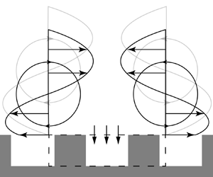
  $\epsilon \ll 1$ is the ratio between the characteristic length scale of the surface and the system (e.g. channel height). However, the transpiration term in the TRM can also be derived from a mass conservation argument, without any use of asymptotic expansions (Lacis et al. Reference Lacis, Sudhakar, Pasche and Bagheri2020). The physical picture depicting this argument is shown in figure 1(a), where a control volume is indicated by the dashed line. Due to mass conservation in this control volume, the varying slip velocity experienced by the flow as it moves over the textured surface must be balanced by a proportional transpiration. A similar reasoning was employed by García-Mayoral & Jiménez (Reference García-Mayoral and Jiménez2011) in deriving the transpiration velocity for flow over riblets. A picture more relevant for near-wall turbulence is sketched in figure 1(b), where two counter-rotating quasi-streamwise vortices and a control volume (dashed line) are shown in the cross-plane. The spanwise slip velocity due the presence of the vortices results in a flux through the vertical faces of the control volume; the difference between these fluxes must then be compensated by a flux through the horizontal face of the control volume, leading to the occurrence of transpiration.

Figure 1. Conceptual illustration of the mass conservation argument for transpiration generation. In ( $a$), the streamwise slip velocity at the crest plane of the textured surface varies in the streamwise direction. Consequently, the in-going and out-going streamwise fluxes through the vertical faces of the control volume (dashed lines) will differ, which due to mass conservation induces a transpiration. ( $b$) Shows the displacement of quasi-streamwise vortices towards the textured surface due to the relaxation of both spanwise no-slip and wall-normal impermeability. The varying spanwise slip velocity at the crest plane results in a net out-going spanwise flux in the control volume, which has to be compensated by transpiration.
To the best of the authors’ knowledge, transpiration boundary conditions have not been thoroughly investigated for the aim of modelling roughness. This is despite the fact that studies of turbulent flow over regular and random roughness (Orlandi & Leonardi Reference Orlandi and Leonardi2006; Orlandi et al. Reference Orlandi, Leonardi and Antonia2006; Forooghi et al. Reference Forooghi, Stroh, Schlatter and Frohnapfel2018a) have established that greater levels of drag are driven by a pronounced presence of wall-normal velocity fluctuations within the roughness region. It should, however, be mentioned that, in the context of manipulating near-wall turbulence, Gómez-de-Segura et al. (Reference Gómez-de-Segura, Fairhall, MacDonald, Chung and García-Mayoral2018), Gómez-de-Segura & García-Mayoral (Reference Gómez-de-Segura and García-Mayoral2020) and Ibrahim et al. (Reference Ibrahim, Gómez-de-Segura, Chung and García-Mayoral2021) investigated Robin boundary conditions of Navier-slip form for all three velocity components
 \begin{equation} u = \ell_x \left.\frac{\partial u}{ \partial y}\right\vert_{y=0},\quad w = \ell_z \left.\frac{\partial w}{ \partial y}\right\vert_{y=0},\quad v = \ell_y \left.\frac{\partial v}{ \partial y}\right\vert_{y=0}.\end{equation}
Note that, for isotropic transpiration, i.e.  $m_x = m_z$, the TRM transpiration condition (2.5) becomes the same as the transpiration condition of (2.6a–c).
The boundary condition for the wall-normal velocity (2.5) can be rewritten by substituting the wall-parallel velocities with their respective slip boundary conditions (2.3)–(2.4), giving
 \begin{equation} v ={-}m_x\ell_x \left.\frac{\partial^{2} u}{ \partial x \partial y}\right\vert_{y=0} - m_z\ell_z \left.\frac{\partial^{2} w}{ \partial z \partial y}\right\vert_{y=0}. \end{equation}
In this form, the transpiration velocity's definition as being due to the variation of the shear rates of the wall-parallel velocities becomes explicit. The terms  $m_x\ell _x=(m\ell )_x$ and $m_z\ell _z=(m\ell )_z$ are the streamwise and spanwise transpiration factors, respectively. These factors contain the compound effect of slip and transpiration lengths and effectively measure the momentum exchange across the crest plane of the roughness. For example, the spanwise transpiration factor can be increased either through a larger spanwise slip length, $\ell _z$, or through a larger spanwise transpiration length, $m_z$. The latter allows a deeper penetration of wall-normal momentum into the texture, while the former indicates a deeper distance below the crest plane before the spanwise velocity component diminishes. Both of these effects increase momentum transport into the roughness region. Finally, it should be emphasized that the TRM models the surface homogeneously and is applied at all locations on the wall using the same coefficients i.e. it is applied uniformly.
3. TRM coefficients and virtual origins
Given appropriate TRM coefficients ( $\ell _x, \ell _z, m_x, m_z$), one may impose the TRM boundary conditions (2.3)–(2.5) to induce the macroscopic effects of a textured surface on the overlying flow. Section 3.1 discusses two approaches to determine the TRM coefficients of a given textured surface; a priori through a so-called unit-cell approach or a posteriori by matching DNS data. Section 3.2 describes the approach of characterizing the modification of turbulence in terms of the virtual origins of different flow quantities (Ibrahim et al. Reference Ibrahim, Gómez-de-Segura, Chung and García-Mayoral2021). If turbulence remains overall similar to that of canonical wall-bounded flow (smooth-wall like), the roughness function (a measure of drag change) is directly quantifiable in terms of the virtual origins of the mean flow and the turbulence.
3.1. Obtaining slip and transpiration lengths for non-smooth surfaces
Assuming that the local flow in the region of a textured surface has  $Re\ll 1$, the slip and transpiration lengths of the TRM boundary conditions can be obtained by carrying out a Stokes flow analysis (Bottaro Reference Bottaro2019; Lacis et al. Reference Lacis, Sudhakar, Pasche and Bagheri2020). The procedure requires numerical simulations of one or a few surface textures, and thus a relatively small computational box, i.e. a representative element volume (REV) or unit-cell. By an averaging of the flow quantities in the unit-cell, homogenized slip and transpiration lengths associated with that surface can be determined. When the Reynolds number is small, the TRM coefficients are a property of the surface alone, and independent of the dynamics of the overlying flow.
An attempt to understand the accuracy of the Stokes-based unit-cell approach for modelling roughness in turbulent flows was made by Lacis et al. (Reference Lacis, Sudhakar, Pasche and Bagheri2020). The surface was comprised of collocated cuboids of height  $k^{+}\approx 7$ (more specifications of the surface are found in figure 11 and table 5 of Lacis et al. Reference Lacis, Sudhakar, Pasche and Bagheri2020). A Stokes analysis in a REV containing a single cuboid provided a slip length of $\ell =\ell _x^{+}=\ell _z^{+}=2.0$ and transpiration length of $m=m_x^{+}=m_z^{+}=2.9$. Note that, due to the isotropic distribution of the collocated cuboids, the spanwise and streamwise TRM coefficients obtained from the REV analysis became equal. Lacis et al. (Reference Lacis, Sudhakar, Pasche and Bagheri2020) conducted a channel flow DNS using the TRM with these calculated lengths which, while demonstrating the same effect, did not achieve quantitative agreement with a geometry-resolving DNS featuring the rough surface. Figures 2(a) and 2(b) show, respectively, the mean velocity and Reynolds shear stress for a TRM simulation, which achieve good quantitative agreement with the geometry-resolving data of Lacis et al. (Reference Lacis, Sudhakar, Pasche and Bagheri2020). The coefficients used in this TRM simulation ( $\ell ^{+}=2, m^{+}=6$) were determined a posteriori by comparing TRM simulations with different transpiration lengths to the geometry-resolving DNS data. The results show that the transpiration length obtained using the Stokes-based REV analysis is underestimated. A probable explanation for the underestimated transpiration length is the omission of the small but nonetheless significant advective effects in the REV analysis. The larger transpiration length $m^{+}$ for surfaces exposed to turbulent flow also means a larger transpiration factor, ${{({m}{\ell })}^{+}}$. The latter depends on the volume-averaged flow within the surface texture region (Lacis et al. Reference Lacis, Sudhakar, Pasche and Bagheri2020, equation (2.14)). In turbulent conditions, it can be expected that the flow in between textures is on average larger in magnitude compared with a laminar flow due to enhanced momentum transfer into the rough surface incurred by turbulent mixing.

Figure 2. Top row shows the mean velocity ( $a$) and Reynolds shear stress ( $b$) profiles for —, smooth-wall; — $\!{\bullet }\!$— (red bullet dashed), geometry-resolving DNS of Lacis et al. (Reference Lacis, Sudhakar, Pasche and Bagheri2020); — $\!\blacksquare$— (green square dashed) DNS with the TRM coefficients ( $\ell ^{+}=2, m^{+}=6$). For the same data, the bottom row shows the shifted mean velocity ( $c$) and Reynolds shear stress ( $d$) profiles for the origin set to $y^{+} = {-\ell _{uv}}^{+}$ and scaled with its associated friction velocity using (3.3).
In contrast to the transpiration, the Stokes-based estimation of the slip length  $\ell ^{+}=2.0$ does not differ from that belonging to the TRM simulation which matches the geometry-resolving DNS. Investigations of Fairhall et al. (Reference Fairhall, Abderrahaman-Elena and García-Mayoral2019) using slip-only boundary conditions to model SHS have shown that Stokes flow analysis provides accurate estimates for textures with characteristic lengths ${L^{+}}\lesssim 5$, which correspond to slip lengths ${{\ell }^{+}}\lesssim 2$. For larger textures, advective effects start to become significant. However, performing laminar flow simulations in an REV extends the validity of the estimates up to ${L^{+}}\lesssim 15$. Abderrahaman-Elena et al. (Reference Abderrahaman-Elena, Fairhall and García-Mayoral2019) demonstrated a similar extent of validity for slip lengths calculated for roughness. Assessing whether laminar flow analysis resolves the discrepancy of the Stokes-estimated transpiration length has yet to be carried out and is not part of this work's objectives.
In the remainder of this study, the transpiration length is determined by matching the results of TRM simulations to those of geometry-resolving DNS, as was demonstrated in figures 2(a) and 2(b). In general, this is not a practical approach to obtain the TRM coefficients for a given surface since it requires performing several simulations. However, it is appropriate for addressing the purpose of the present work; namely, to demonstrate the applicability of the TRM and gauge the extent of its validity for modelling physically realizable drag-increasing surfaces.
3.2. Drag change in terms of virtual origins
The virtual-origin framework of Ibrahim et al. (Reference Ibrahim, Gómez-de-Segura, Chung and García-Mayoral2021) provides a method of quantifying drag change based on how small surface textures affect the near-wall turbulence structures. The measure of drag change adopted here is the roughness function  $\Delta U^{+}$. As is conventionally understood, the presence of surface textures causes a vertical shift, $\Delta U^{+}$, of the logarithmic region of the mean velocity profile (Clauser Reference Clauser1956),
 \begin{equation} {U}^{+} = \frac{1}{\kappa}\log\left ({y}^{+}\right) + B + \Delta U^{+}. \end{equation}
Here,  $\kappa \approx 0.4$ is the von Kármán constant and $B\approx 5.0$ is the offset of the logarithmic region from the wall origin. A negative $\Delta U^{+}$ indicates a downward shift of the mean velocity profile which is observed for drag-increasing surfaces. This shift is considered to be the appropriate quantity in measuring the drag change caused by textures small enough for their effect to remain limited to the near-wall region. As long as the characteristic texture size remains the same when scaled in inner units, the corresponding value of $\Delta U^{+}$ will also remain fixed regardless of Reynolds number (Spalart & McLean Reference Spalart and McLean2011; García-Mayoral et al. Reference García-Mayoral, Gómez-de-Segura and Fairhall2019).
The virtual-origin framework quantifies the roughness function in terms of two so-called virtual origins
 \begin{equation} \Delta U^{+}={\ell_U}^{+}-{\ell_{T}}^{+}. \end{equation}
Here,  ${\ell _U}^{+}$ is the virtual origin of the mean flow and ${\ell _T}^{+}$ the virtual origin of near-wall turbulence. The concept of separate virtual origins for the mean and turbulent components of the flow was originally established by Luchini (Reference Luchini1996), with ${\ell _U}^{+}$ describing an imaginary impermeable smooth wall perceived by the mean flow at the position ${y^{+}=-\ell _{U}}^{+}$ and ${\ell _T}^{+}$ describing the same for the near-wall turbulence. The physical reasoning behind this is that the turbulence dynamics in this region is driven by the quasi-streamwise vortices (figure 1b), which undergo a displacement due to a weakening of both cross-flow shear and impermeability owing to the presence of small surface textures. This is due to the first-order effect of the vortices at the boundary plane being the generation of cross-flow shear while transpiration is their second-order effect (Gómez-de-Segura & García-Mayoral Reference Gómez-de-Segura and García-Mayoral2020; Ibrahim et al. Reference Ibrahim, Gómez-de-Segura, Chung and García-Mayoral2021). Thus, the turbulence undergoes a rigid translation by a distance ${\ell _T}^{+}$ but otherwise remains smooth-wall like. This is analogous to it perceiving a smooth wall at $y=-{\ell _T}^{+}$.
As demonstrated by Gómez-de-Segura & García-Mayoral (Reference Gómez-de-Segura and García-Mayoral2020), once the origin for the wall-normal coordinate is set at  $y^{+}={-\ell _T}^{+}$ and the friction velocity calculated at this origin
 \begin{equation} {u_{\tau}}\rvert_{y={-\ell_{T}}} = {u_{\tau}}\rvert_{y=0}\sqrt{ \cfrac{\delta + \ell_{T}}{\delta}}, \end{equation}
is used for rescaling the flow quantities, the resulting mean velocity profile mirrors that of a smooth-wall turbulent flow and is only offset from it by  $\Delta U^{+}={\ell _U}^{+}-{\ell _T}^{+}$.
Virtual origins can be defined for the streamwise ( ${\ell _u}^{+}$), spanwise ( ${\ell _w}^{+}$) and wall-normal ( ${\ell _v}^{+}$) velocities as well as for the Reynolds shear stress ( ${\ell _{uv}}^{+}$). Ibrahim et al. (Reference Ibrahim, Gómez-de-Segura, Chung and García-Mayoral2021) established that the appropriate choice for $\ell _T^{+}$ is the virtual origin of the Reynolds shear stress, i.e. ${\ell _T}^{+}={\ell _{uv}}^{+}$, ultimately giving
 \begin{equation} \Delta U^{+}={\ell_U}^{+}-{\ell_{uv}}^{+} . \end{equation}
Figure 2(c) demonstrates this for the collocated cuboids of Lacis et al. (Reference Lacis, Sudhakar, Pasche and Bagheri2020) and thus confirms that the turbulence modification caused by the surface texture in this case merely amounts to a displacement of the near-wall vortices. The choice of turbulence origin being  ${\ell _T}^{+}={\ell _{uv}}^{+}$ is also commensurate with the fact that for the mean flow, the stress terms which appear in the mean momentum equation are those of viscous and Reynolds shear stress, with the latter being non-existent at the wall. This associates the wall for canonical smooth-wall turbulence with the condition that $\overline {u^{\prime }v^{\prime }}^{+}=0$. It follows from this line of reasoning that if the mean and turbulent components of the flow undergo displacements but remain otherwise smooth-wall like, then the proper choice of wall-normal origin will be $y^{+}={-\ell _{uv}}^{+}$, the plane where $-\overline {u^{\prime }v^{\prime }}^{+}$ perceives an imaginary smooth wall.
The relation between the roughness function and virtual origins (3.4) can be derived from the mean momentum or Reynolds-averaged Navier–Stokes (RANS) equation. The procedure is detailed in Gómez-de-Segura & García-Mayoral (Reference Gómez-de-Segura and García-Mayoral2019) and may be referred to by the interested reader. In this work, the virtual origin framework has been leveraged when analysing the results of turbulent channel flow DNS where the TRM boundary conditions have been used. The virtual origins are obtained a posteriori. Following Ibrahim et al. (Reference Ibrahim, Gómez-de-Segura, Chung and García-Mayoral2021),  ${\ell _U}^{+}$ corresponds to the slip velocity, ${U_{slip}}^{+}$, at $y^{+}=0$, while ${\ell _{uv}}^{+}$ represents the shift of $-\overline {u^{\prime }v^{\prime }}^{+}$ relative to that of a smooth-wall solution giving the best fit in the region of $10 < y^{+} < 25$. The virtual origins of the velocity fluctuations, ${\ell _u}^{+}$, ${\ell _w}^{+}$ and $\ell ^{+}_v$, also calculated a posteriori, were obtained via extrapolation of their root-mean-square (r.m.s.) profiles. The curvature of the profiles were taken into account and hence linear extrapolation was not used. This is particularly important for the ${v^{\prime }}^{+}$ profile as it is strongly quadratic very close to the boundary.
4. Numerical method
The numerical solver used is based on the finite volume method where the incompressible Navier–Stokes equations (2.1)–(2.2) are spatially discretized using second-order central finite differences on a Cartesian grid with a staggered arrangement. Temporal integration of the solution utilizes a fully explicit triple sub-step Runge–Kutta scheme (Spalart, Moser & Rogers Reference Spalart, Moser and Rogers1991; Wesseling Reference Wesseling2009) in a fractional-step pressure correction method (Kim & Moin Reference Kim and Moin1985; Armfield & Street Reference Armfield and Street2002). The discretized equations in operator form then read
 \begin{gather} \boldsymbol{u}^{*} = \boldsymbol{u}^{k} + \Delta t({\alpha_{k}}(\boldsymbol{\mathsf{A}}\boldsymbol{u}^{k} + \nu\boldsymbol{\mathsf{L}}\boldsymbol{u}^{k}) + {\beta_{k}}(\boldsymbol{\mathsf{A}}\boldsymbol{u}^{k-1} + \nu\boldsymbol{\mathsf{L}}\boldsymbol{u}^{k-1})-{\gamma_{k}}\boldsymbol{\mathsf{G}}p^{k-1/2}), \end{gather}
 \begin{gather}\boldsymbol{\mathsf{L}}{\varPhi} = \frac{\boldsymbol{\mathsf{D}}\boldsymbol{u}^{*}}{{\gamma_{k}}\Delta t}, \end{gather}
 \begin{gather}\boldsymbol{u}^{k} = \boldsymbol{u}^{*} - {\gamma_{k}}\Delta t\boldsymbol{\mathsf{G}}{\varPhi}, \end{gather}
 \begin{gather}p^{k+1/2} = p^{k-1/2} + {\varPhi}. \end{gather}
The Runge–Kutta sub-step is designated by  $k = 1, 2, 3$ with $k = 1$ corresponding to time step $n$ and $k = 3$ to $n + 1$; $\boldsymbol{\mathsf{A}}$, $\boldsymbol{\mathsf{L}}$, $\boldsymbol{\mathsf{G}}$ and $\boldsymbol{\mathsf{D}}$ represent the discrete advection, Laplacian, gradient and divergence operators. The term $\boldsymbol {u^{*}}$ is the intermediate velocity and $\varPhi$ is the pressure correction (Kim & Moin Reference Kim and Moin1985; Temam Reference Temam1991). The coefficients of the Runge–Kutta scheme are $\alpha =\{8/15,5/12,3/4\}$, $\beta =\{0,-17/60,-5/12\}$ and $\gamma =\alpha +\beta$. The pressure correction, $\varPhi$, is calculated by solving a Poisson equation in Fourier space using a computationally efficient fast Fourier transform (FFT)-based solver (Costa Reference Costa2018). It then acts as a Lagrange multiplier, projecting $\boldsymbol {u^{*}}$ onto a divergence-free field such that it satisfies the incompressibility constraint (2.2). For the temporal integration using the Runge–Kutta scheme, the following stability criteria given in Wesseling (Reference Wesseling2009) is applied:
 \begin{equation} \frac{\Delta t}{\mathrm{CFL}} = \mathrm{min}\left\{{ \frac{1.65}{4\nu}\left({{\frac{1}{{ \Delta x}^{2}}+{\frac{1}{\Delta{y}^{2}}}+\frac{1}{{\Delta{z}}^{2}}}}\right)^{{-}1}, \frac{\sqrt{3}}{\vert{u}\vert{\Delta x}^{{-}1} + \vert{v}\vert{\Delta y}^{{-}1} + \vert{w}\vert{\Delta z}^{{-}1}} }\right\}, \end{equation}
with  $\mathrm {Courant-Friedrichs-Lewy (CFL)} = 0.5$ being used. The computational domain has conventional dimensions of $L_x = 2{\rm \pi} \delta$, $L_y = 2\delta$ and $L_z = {\rm \pi}\delta$, where $\delta$ is the channel half-height. The numbers of grid points are $N_x = 192$, $N_y = 144$ and $N_z = 160$; evenly spaced along $x$,
$x$,  $z$ and unevenly along $y$ using a hyperbolic tangent function. The spatial resolution in the horizontal directions are $\Delta x^{+} = 5.9$ and $\Delta z^{+} = 3.5$, while the wall-normal resolution varies from $\Delta y^{+} = 0.6$ at the boundaries to $\Delta y^{+} = 4.3$ at the channel mid-plane. Parallelization of the computational domain is achieved through a two-dimensional pencil-like decomposition using the 2DECOMP&FTT library (Li & Laizet Reference Li and Laizet2010), which uses MPI. Simulations were conducted at a fixed friction Reynolds number of $Re_{\tau }={u_{\tau }\delta }/{\nu }=180$, with the flow driven by an imposed constant mean pressure gradient. Two simulations at $Re_{\tau }=550$ were also conducted, maintaining the previously mentioned spatial resolutions but requiring $N_x = 448$, $N_y = 448$ and $N_z = 448$ grid points. Statistically converged smooth-wall solutions were used as the initial conditions and the simulations were advanced for $110\,\delta /u_{\tau }$, with statistics gathered over at least $50\,\delta /u_{\tau }$.
The boundary conditions along  $x$ and $z$ are periodic while the TRM boundary conditions are imposed on both domain boundaries at $y=[0,2\delta ]$. The slip velocity conditions for $u$ and $w$ (2.3)–(2.4) as well as the transpiration condition for $v$ (2.7) are implemented explicitly, making the latter directly coupled to the derivatives of the former two. To avoid numerical instabilities and ensure that the resulting slip and transpiration velocities at each time step of the simulation satisfy the incompressibility condition, a somewhat non-trivial procedure was employed which is briefly explained here for the benefit of the interested reader. A complete Runge–Kutta loop (4.2)–(4.4) is first executed using the solution of time step $n$ to obtain the solution in the interior of the domain for time step $n + 1$. An inner loop then uses the updated $u$ and $w$ velocities and iterates over the transpiration boundary condition (2.7), relaxing $v$ at $y=[0,2\delta ]$ to its final value for time step $n + 1$ by using the preceding transpiration velocity (at time step $n$) as its initial guess. The iterations continue until a convergence criterion is satisfied, which is that the sum of squared residuals of the transpiration velocity at the boundaries should be less than ${O}(10^{-5})$. The number of iterations required ranged from 9 to 20 for the weakest and strongest transpiration cases that were examined, with the additional computational cost per iteration estimated as being approximately $0.7$ s in wall-clock time. Also, only the pressure fluctuations at the boundaries are retained to ensure zero net mass flux through them, as was similarly done by Jiménez et al. (Reference Jiménez, Uhlmann, Pinelli and Kawahara2001).
The numerical solver and the implementation of the boundary conditions were validated and the results are reported in Appendix A, along with an assessment of solution grid independence. The validation of the TRM boundary conditions’ implementation was carried out against matching cases from Gómez-de-Segura & García-Mayoral (Reference Gómez-de-Segura and García-Mayoral2020) and Ibrahim et al. (Reference Ibrahim, Gómez-de-Segura, Chung and García-Mayoral2021), where velocity boundary conditions in the form of (2.6a–c) had been used. The numerical method used in those studies employs the block lower-upper (LU) decomposition suggested by Perot (Reference Perot1993). This results in an implicit implementation of the boundary conditions while also avoiding the need for boundary conditions to be defined for the intermediate variables of the fractional-step method, thereby providing a greater degree of consistency.
5. DNS of turbulent channel flow with the TRM
In § 5.1, the results from a number of TRM-based DNS conducted by imposing different conditions ( $\ell _x, \ell _z, m_x, m_z$) are reported and analysed. This is to understand how turbulence is gradually modified as the TRM coefficients are varied, and if the observed modifications are consistent with those of textured surfaces in the transitionally rough regime. The actual connection of the TRM coefficients to physical textured surfaces is addressed in § 6.
As explained in § 3.2, the concept of virtual origins feature heavily in the works of Gómez-de-Segura et al. (Reference Gómez-de-Segura, Fairhall, MacDonald, Chung and García-Mayoral2018), Gómez-de-Segura & García-Mayoral (Reference Gómez-de-Segura and García-Mayoral2020) and the more recent work of Ibrahim et al. (Reference Ibrahim, Gómez-de-Segura, Chung and García-Mayoral2021) which formalized it into a framework. This will naturally invite comparisons to be made with the results herein and therefore a cross-analysis has been gathered in Appendix B for the interested reader, but omitted here for the sake of brevity.
The cases through which the TRM is examined are listed in table 1. Each case is denoted with  ${\rm L}\langle \cdot \rangle {\rm M}\langle \cdot \cdot \rangle$, where the digit following L refers to the slip lengths, ${\ell _x}^{+}$ and ${\ell _z}^{+}$, while the letter and digit following M denotes the transpiration length(s) imposed and their values; X for ${m_x}^{+}\neq 0$, ${m_z}^{+}=0$; Z for ${m_x}^{+}=0$, ${m_z}^{+}\neq 0$ and no letter for $m^{+}={m_x}^{+}={m_z}^{+}$. Note that, for all simulations considered, the streamwise and spanwise slip lengths are equal ( $\ell ^{+}={\ell _x}^{+}={\ell _z}^{+}$) and anisotropy is investigated only for the transpiration lengths.
Table 1. Summary of the TRM simulations performed with their slip ( ${\ell _{x}}^{+}, {\ell _{z}}^{+}$) and transpiration lengths ( ${m_{x}}^{+}$, ${m_{z}}^{+}$). Here, $Re_{\tau }$ is based on ${u_{\tau }}\rvert _{y=0}$ and $Re_{\tau }^{\delta '}$ on ${u_{\tau }}\rvert _{y={-\ell _{uv}}}$ with $\delta ' = \delta + {\ell _{uv}}^{+}$. The virtual origins of the velocity fluctuations, the mean flow and the Reynolds shear stress ( ${\ell _u}^{+}, {\ell _w}^{+}, {\ell _v}^{+}, {\ell _U}^{+}, {\ell _{uv}}^{+}$) are calculated a posteriori, as established in § 3.2. The reported roughness function $\Delta U^{+}$ is computed from the virtual origins ${\ell _U}^{+}$ and ${\ell _{uv}}^{+}$ using (3.4). The first group of 9 simulations used the TRM with isotropic transpiration lengths at $Re_\tau =180$ and $Re_\tau =550$. The second group of 5 simulations used the TRM with only streamwise transpiration imposed while the last group used the TRM with only spanwise transpiration imposed.

5.1. TRM with isotropic transpiration lengths
Cases with equal transpiration lengths are considered first (the 9 initial rows in table 1). This implies that the contributions made to the overall transpiration by the streamwise and spanwise flows are of equal proportion, with no preferentiality given to either.
5.1.1. Smooth-wall-like regime
The zero-transpiration case of L2M0 is similar to the many slip-only simulations found throughout the literature (Min & Kim Reference Min and Kim2004; Fukagata et al. Reference Fukagata, Kasagi and Koumoutsakos2006; Busse & Sandham Reference Busse and Sandham2012; Gómez-de-Segura & García-Mayoral Reference Gómez-de-Segura and García-Mayoral2020). It causes a slight reduction in drag, as evident by the excess momentum it has relative to the smooth-wall solution ( $\Delta U^{+}=0.7$). Indeed, the virtual origin of the mean flow ( ${\ell _U}^{+}=2$) is larger than the virtual origin of the Reynolds shear stress ( ${\ell _{uv}}^{+}=1.3$), which, according to (3.4), will result in a decrease of drag. Note that, while the impermeability condition is maintained for this case, and hence $\overline {u^{\prime }v^{\prime }}^{+}=0$ at the boundary, it's near-wall distribution undergoes a change, which results in ${\ell _{uv}}^{+}=1.3$. The drag-increasing effect here is due to the imposed spanwise slip, which, as argued in § 3.2, causes the quasi-streamwise vortices to become displaced and generate wall-normal mixing in the region closer to the boundary plane.
Figure 3(a) shows the mean velocity profiles of simulations with different slip and transpiration lengths. Increasing the streamwise slip length ( ${\ell _{x}}^{+}\in [2, 5, 10]$) causes the mean flow virtual origin ( ${\ell _U}^{+}$) to become deeper. Further away from the wall the mean velocity either conforms to the smooth-wall profile (drag neutral) or becomes shifted downwards (drag increase) depending on the size of imposed transpiration length ( ${m^{+}}\in [2,5,10]$). A non-zero transpiration length in case L2M2 results in both ${v^{\prime }}^{+}$ and $-\overline {u^{\prime }v^{\prime }}^{+}$ having finite values at the boundary plane (red solid line in figure 3b,d). Increased transpiration leads to greater Reynolds shear stress closer to the boundary and a decrease of the drag reduction observed in case L2M0, neutralizing it almost entirely ( ${\ell _U}^{+}={\ell _{uv}}^{+}=2$ and $\Delta U^{+}=0$ for L2M2). Increasing the transpiration lengths further in case L2M5 ( ${\ell }^{+}=2, {m}^{+}=5$), such that they now exceed their corresponding slip lengths, amounts to a downward shift of the velocity profile ( $\Delta U^{+}=-1$) and drag increase. As can be observed in figures 3(a) and 3(d) (green solid line), case L2M5 results in greater amounts of Reynolds shear stress in the near-boundary region ( ${\ell _{uv}}^{+}=2.9$), whereas the mean velocity slip ( ${\ell _U}^{+}=1.9$) has essentially the same value of the lower transpiration case L2M2. Therefore, the increase in Reynolds shear stress overcomes the beneficial effect of the mean velocity slip and leads to a momentum deficit of the flow ( $\Delta U^{+}<0$).

Figure 3. Mean velocity ( $a$), r.m.s. velocity fluctuation ( $b$–
$b$– $c$) and Reynolds shear stress ( $d$) profiles of ${\rm L}\langle \cdot \rangle {\rm M}\langle \cdot \rangle$ cases: — (red solid line), L2M2; — (green solid line), L2M5; — (blue solid line), L5M5; — (magenta solid line), L5M10; — (cyan solid line), L10M10; —, smooth-wall data. Arrows indicate increasing $m^{+}$.
The level of transpiration generated due to the TRM (2.3)–(2.5) is influenced by slip lengths imposed on the tangential velocity components. To demonstrate this, for case L5M5 the transpiration lengths of L2M5 have been kept but the slip lengths increased by a factor of  $2.5$. Since the transpiration factors in (2.7) contain slip lengths, an increase in the latter modifies the intensity of wall-normal fluctuations at the boundary plane (blue solid line in figure 3b). Greater levels of wall-normal fluctuations in turn result in greater levels of Reynolds shear stress (figure 3d). This is also reflected in the calculated virtual origins; with ${\ell _v}^{+}=6.6$ and ${\ell _{uv}}^{+}=4.7$ for case L5M5, while ${\ell _v}^{+}=5.8$ and $\ell ^{+}_{uv}=2.9$ for case L2M5.
5.1.2. Deviations from smooth-wall turbulence
A pertinent question here is the extent of the TRM's applicability as a model for transitionally rough flows beyond the initial regime of smooth-wall-like turbulence. The transpiration length was therefore increased to  $m^{+}=10$ for different slip lengths to assess the resulting modification of near-wall turbulence. The high-transpiration cases in table 1 are L5M10 (magenta solid line) and L10M10 (cyan solid line), shown in figure 3.
Case L5M10 results in  $\Delta U^{+}=-2.9$, which is nearly half-way into the transitionally rough regime (assuming the fully rough regime to correspond to $\Delta U^{+}\approx 6$, as described by Jiménez Reference Jiménez2004). The resulting virtual origins of the mean flow and Reynolds shear stress are ${\ell _U}^{+}=3.7$ and ${\ell _{uv}}^{+}=6.6$. The latter implies a significant modification of the near-wall turbulence. Compared with the cases with ${m^{+}}<10$, the intensities of ${v^{\prime }}^{+}$ and ${w^{\prime }}^{+}$ have increased while that of ${u^{\prime }}^{+}$ has decreased, demonstrating a move towards turbulence isotropization (figure 3b,c). The near-wall distribution of $-\overline {u^{\prime }v^{\prime }}^{+}$ also undergoes a noticeable outward rise compared with its smooth-wall counterpart (figure 3d). An even stronger modification of the turbulence is observed for case L10M10 ( $\ell ^{+}_{uv}=7.7$), although the drag increase ( $\Delta U^{+}=-1.6$) is smaller owing to the large mean flow slip ( $\ell _U^{+}=6.1$).
Figure 4 shows that smooth-wall statistics are recoverable for the majority of the cases considered thus far after accounting for the virtual-origin effect. However, differences from smooth-wall turbulence are noticeably present in cases L5M10 and L10M10 (figure 4b).
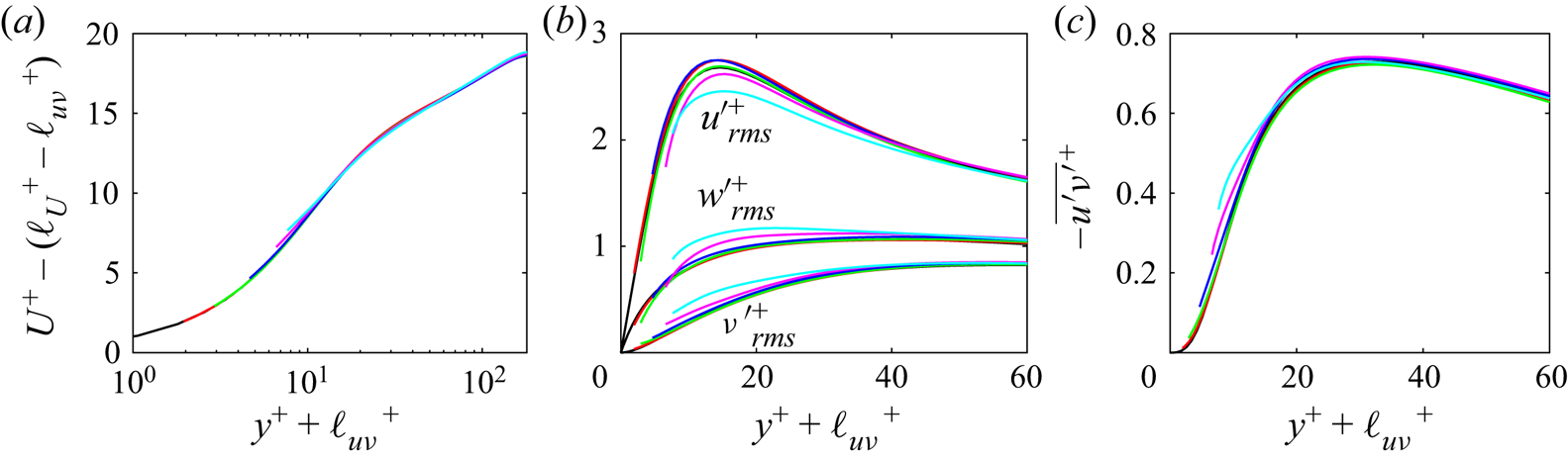
Figure 4. Mean velocity ( $a$), r.m.s. velocity fluctuation ( $b$) and Reynolds shear stress ( $c$) profiles with the origin at ${y}^{+} = -{\ell _{uv}}^{+}$ and rescaled with ${u_{\tau }}$ at that plane: — (red solid line), L2M2; — (green solid line), L2M5; — (blue solid line), L5M5; — (magenta solid line), L5M10; — (cyan solid line), L10M10; —, smooth-wall data.
To better determine the extent of such differences the pre-multiplied energy spectra may be examined. Figure 5 shows (from top to bottom) the energy spectra for L10M10, L5M5, L2M5 and L2M2. The spectra of L2M2 and L2M5 conform to the smooth-wall spectra closely, reaffirming that the turbulence is smooth-wall like in these cases. In contrast, the spectra of case L5M5 exhibit differences for  ${v}^{2}$ and ${w}^{2}$ (figure 5f,g), while that of its Reynolds shear stress (figure 5h) remains largely smooth-wall like. Case L10M10 shows large differences across all spectra, consistent with the deviations observed in figure 4. The deviations observed in the co-spectra of the wall-normal fluctuations are typical for surfaces that induce a Kelvin–Helmholtz type of instability. This is further examined in § 7.3 where it is also observed for cases with anisotropic transpiration lengths.

Figure 5. Pre-multiplied two-dimensional spectral densities of  ${u}^{2}$, ${v}^{2}$, ${w}^{2}$ and ${uv}$: L10M10 ( $a$–
$a$– $d$); L5M5 ( $e$–
$e$– $h$); L2M5 ( $i$–
$i$– $l$); L2M2 ( $m$–
$m$– $p$); shaded regions are the smooth-wall solution at $y^{+}\approx 15$ and solid lines are the TRM cases at $y^{+}+{\ell _{uv}}^{+}\approx 15$ scaled using the $u_{\tau }$ at $y^{+}=-{\ell _{uv}}^{+}$.
5.1.3. Reynolds number scaling
As described in § 3.2,  $\Delta U^{+}$ should be independent of Reynolds number so long as the characteristic size of a given surface texture remains constant in inner units. Hence, for Robin boundary conditions, which impose lengths of different magnitude on the velocity components, the effect should scale in inner units with Reynolds number. This is investigated for cases L2M2 and L5M5 by simulating them at a higher Reynolds number but keeping their slip and transpiration lengths fixed in inner units. These higher Reynolds number cases are designated L2M2HR and L5M5HR in table 1. Both were simulated at $Re_{\tau } = 550$ and the data are shown in figure 6. The mean velocity and Reynolds shear stress achieve a similar level of conformity to their respective smooth-wall solutions once the origin is shifted to $y^{+} = -{{\ell }_{uv}}^{+}$ and the flow quantities are rescaled with the friction velocity at that position. A similar agreement is observed for the r.m.s. velocity fluctuations. The mean velocity shift, $\Delta U^{+} = {{\ell }_U}^{+} - {{\ell }_{uv}}^{+}$, for the two sets of slip and transpiration lengths remain the same at both Reynolds numbers, demonstrating that their effect is independent of Reynolds number.

Figure 6. Mean velocity, r.m.s. velocity fluctuation and Reynolds shear stress profiles of the  ${\rm L}\langle \cdot \rangle {\rm M}\langle \cdot \rangle {\rm HR}$ cases. Origin at ${y}^{+} = 0$ ( $a$–
$a$– $c$), origin at ${y}^{+} = -{\ell _{uv}}^{+}$ ( $d$–
$d$– $f$): — (red solid line), L2M2HR; — (blue solid line), L5M5HR; – – (red dashed line), L2M2; – – (blue dashed line), L5M5; —, smooth-wall data at $Re_{\tau } = 550$; – –, smooth-wall data at $Re_{\tau } = 180$.
6. Applicability to geometrical roughness
It has thus far been demonstrated that the TRM can cause changes in near-wall turbulence which in turn leads to changes in drag. In this section, the applicability of the TRM at reproducing the effect of actual rough surfaces in the transitionally rough turbulence regime is assessed. The potential of this had been demonstrated by Lacis et al. (Reference Lacis, Sudhakar, Pasche and Bagheri2020) as discussed in § 3.1. Here, a more in-depth analysis is provided by considering a number of different rough surfaces.
6.1. Matching TRM with geometry-resolving data
Several geometries have been chosen from Abderrahaman-Elena et al. (Reference Abderrahaman-Elena, Fairhall and García-Mayoral2019), who performed DNS of turbulent channel flow over textured surfaces. The texture geometry of the main case chosen for evaluation is depicted schematically in figure 7. The surface consists of a homogeneous distribution of collocated posts of height  $k$ with equal streamwise and spanwise pitch lengths ( $s_x=s_z$). The data of Abderrahaman-Elena et al. (Reference Abderrahaman-Elena, Fairhall and García-Mayoral2019) also have a triple decomposition applied to them such that the footprint of the roughness region is removed from the turbulence statistics. This makes them more suitable for comparison as the TRM simulations likewise do not have a region occupied by any discrete geometry. It should be emphasized, however, that this does not modify the statistics above the roughness region or the macro-scale effect of the roughness on the bulk flow. The characteristics of the geometries considered (C06-C12) are listed in table 2.

Figure 7. Roughness pattern of the DNS cases of Abderrahaman-Elena et al. (Reference Abderrahaman-Elena, Fairhall and García-Mayoral2019) consisting of collocated posts.
Table 2. Characteristics of the geometry-resolving (Geo-Res) DNS cases of Abderrahaman-Elena et al. (Reference Abderrahaman-Elena, Fairhall and García-Mayoral2019) for the roughness pattern depicted in figure 7. The definitions of the various terms are as described in table 1 with the exception of  $\Delta U^{+}$, which, here, is simply the mean velocity shift calculated at the channel centreline without any coordinate shift or rescaling having been applied. Data adapted from Abderrahaman-Elena et al. (Reference Abderrahaman-Elena, Fairhall and García-Mayoral2019).
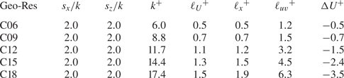
Owing to the homogeneous pattern of the roughness, both the streamwise and spanwise slip lengths used in the TRM boundary conditions are set equal to that calculated by Abderrahaman-Elena et al. (Reference Abderrahaman-Elena, Fairhall and García-Mayoral2019) for the mean streamwise flow ( $\ell ^{+}=\ell ^{+}_x=\ell ^{+}_z$). The values of $\ell _x^{+}$ are reported in table 2. The transpiration lengths, $m^{+}={m_{x}}^{+}={m_{z}}^{+}$, are incrementally increased until the displacement of the Reynolds shear stress, i.e. the turbulence virtual origin ${\ell _{uv}}^{+}$, closely matches those reported by Abderrahaman-Elena et al. (Reference Abderrahaman-Elena, Fairhall and García-Mayoral2019).
Figure 8 demonstrates the process for case C12 by comparing the data of the TRM simulations with the geometry-resolving ones. The transpiration lengths used ranged from  $m^{+}=2$ to $m^{+}=10$. The turbulence statistics produced using $m^{+}=10$ (case L1.2M10 in table 3) agree well with the geometry-resolving DNS data for C12, demonstrating that the TRM is capable of reproducing such transitionally rough effects. All of the TRM cases here fall within the regime of smooth-wall-like turbulence, as evident by the collapse of the Reynolds shear stress profiles onto that of a smooth wall's when adjusted for ${\ell _{uv}}^{+}$ in figure 8(h). It follows that the mean velocity profiles (figure 9b) will also collapse onto the smooth-wall one (figure 9b). Aside from differences in the region closest to the boundary due to each velocity component decaying to a different virtual origin (Abderrahaman-Elena et al. Reference Abderrahaman-Elena, Fairhall and García-Mayoral2019), the fluctuations also collapse onto their smooth-wall counter-parts.

Figure 8. The r.m.s. velocity fluctuation and Reynolds shear stress profiles of cases  ${\rm L}1.2{\rm M}\langle 2\unicode{x2013}10\rangle$. Origin at ${y}^{+} = 0$ ( $a,c,d,e$), origin at ${y}^{+} = -{\ell _{uv}}^{+}$ and rescaled with the corresponding ${u_{\tau }}$ ( $b,f,g,h$). Symbols represent geometry-resolving DNS case C12 from Abderrahaman-Elena et al. (Reference Abderrahaman-Elena, Fairhall and García-Mayoral2019), arrows indicate increasing $m^{+}$.
Table 3. Summary of TRM simulations conducted for comparison with the rough-wall DNS of Abderrahaman-Elena et al. (Reference Abderrahaman-Elena, Fairhall and García-Mayoral2019). The definitions of the various terms are as described in table 1 with the exception of  $\Delta U^{+}$, which follows the definition in table 2.


Figure 9. Mean velocity profiles of cases  ${\rm L}1.2{\rm M}\langle 2\unicode{x2013}10\rangle$. Origin at ${y}^{+} = 0$ ( $a$); origin at ${y}^{+} = -{\ell _{uv}}^{+}$, rescaled with the corresponding ${u_{\tau }}$ and with $\Delta U^{+}={\ell _{U}}^{+}-{\ell _{uv}}^{+}$ subtracted ( $b$). Arrows indicate increasing $m^{+}$.
The TRM simulations corresponding to the remaining geometries C06, C09, C15 and C18 are respectively L0.5M8, L0.7M7, L1.5M12 and L1.9M15, as listed in table 3. In other words, these cases produced similar levels of drag as their geometry-resolving counter-parts from Abderrahaman-Elena et al. (Reference Abderrahaman-Elena, Fairhall and García-Mayoral2019). However, the geometry-resolving DNS cases C15 and C18 exhibit near-wall turbulent behaviour which is no longer smooth-wall like (Abderrahaman-Elena et al. Reference Abderrahaman-Elena, Fairhall and García-Mayoral2019). Therefore, it is important to assess if the corresponding TRM cases can cause similar changes in turbulence and not only a matching change in drag. The comparisons are made in figure 10; some discrepancy exists, most notably for the r.m.s. velocity fluctuations of  $u$ in the near-wall region (figure 10a) where the TRM results have peaks of greater magnitude. The distribution of the $v$ and $w$ r.m.s. velocities match quite well, as do those of the Reynolds shear stresses. Aside from the boundary conditions themselves being the principal source of these discrepancies, other potentially contributing factors may be the higher resolution of the geometry-resolving DNS simulations as well as the solver of those simulations using a pseudo-spectral spatial discretization.

Figure 10. Comparison between the TRM DNS and the geometry-resolving rough-wall DNS of Abderrahaman-Elena et al. (Reference Abderrahaman-Elena, Fairhall and García-Mayoral2019) showing r.m.s. velocity fluctuation ( $a$–
$a$– $c$) and Reynolds shear stress ( $d$) profiles: ${\bullet }$ (blue), C15; ${\blacksquare }$ (red), C18; — (blue solid line), L1.5M12; — (orange solid line), L1.9M15; —, smooth-wall data.
6.2. The role of the transpiration factor
Figure 11(a) shows how the height of the posts (i.e. the roughness height),  $k^{+}$, scales with $(m\ell )^{+}$. A monotonic increase is observed along with a nearly linear proportionality. A larger height of the posts translates to deeper cavities in between them, creating more room for the wall-normal velocity to penetrate below the crest plane. This is the effect quantified by the transpiration length, $m^{+}$. The spacing between the posts, ${s_x}^{+}$ and ${s_z}^{+}$, leads to the existence of a slip velocity at the roughness crests, which is the effect quantified by the slip lengths ${\ell _x}^{+}$ and ${\ell _z}^{+}$. Clearly, changes in the geometrical features of the surface are reflected in the TRM's coefficients ( $\ell ^{+}$, $m^{+}$) in a physically consistent way. In particular, the compound effect of the texture's height and pitch lengths, which determines the overall degree of transpiration that can take place at the crest plane, is captured by the transpiration factor ${(m\ell )}^{+}$.

Figure 11. Height of the collocated posts ( $k^{+}$), roughness function relative to mean velocity slip ( ${-\Delta U^{+}}+{{\ell _{U}}^{+}}$) and the virtual origin of the Reynolds shear stress ( ${\ell _{uv}}^{+}$) as functions of the transpiration factor shown in ( $a$), ( $b$) and ( $c$), respectively: $\bullet$, smooth-wall; $\bullet$ (red), L0.5M8; ${\blacklozenge }$ (green), L0.7M7; ${\blacktriangle }$ (blue), L1.2M10; ${\blacksquare }$ (magenta), L1.5M12; ${\bigstar }$ (cyan), L1.9M15. —, linear fits ${0.204}({m}{\ell })^{+}$, ${0.185}({m}{\ell })^{+}$ and ${0.429}({m}{\ell })^{+}$ in ( $a$), ( $b$) and ( $c$), respectively.
Earlier studies on both regular and random roughness (Orlandi & Leonardi Reference Orlandi and Leonardi2006; Forooghi et al. Reference Forooghi, Stroh, Schlatter and Frohnapfel2018a) have demonstrated a linear relation between the wall-normal velocity fluctuations at the crest plane and the roughness function. A similar relation between the transpiration factor  ${(m\ell )}^{+}$ and the roughness function can be expected. As discussed in § 2, ${(m\ell )}^{+}$ is an effective measure of the volume-averaged (using an appropriate REV) flow within the textured surface. Figure 11(b) shows how the roughness function (reported here relative to the slip velocity, $-\Delta U^{+}+{{\ell _{U}}^{+}}$, following Orlandi & Leonardi Reference Orlandi and Leonardi2006; Abderrahaman-Elena et al. Reference Abderrahaman-Elena, Fairhall and García-Mayoral2019) scales with the transpiration factor ${(m\ell )}^{+}$. An overall linear proportionality is observed for the TRM simulations that reproduce the collocated posts DNS cases C06-C18 in table 2.
Since the roughness function demonstrates an even stronger linear relation with  ${\ell _{uv}}^{+}$, a linear relation between ${(m\ell )}^{+}$ and ${\ell _{uv}}^{+}$ can also be expected, which is shown in figure 11(c). As will be shown in the next section, the transpiration is predominately driven by changes in spanwise shear, as this leads to the displacement of quasi-streamwise vortices which generate wall-normal fluctuations for canonical turbulence (figure 1b). Since this displacement is quantified by ${\ell _{uv}}^{+}$, the virtual origin of turbulence and the transpiration factor are linearly proportional to each other. This proportionality also persists for the cases which fall outside of the smooth-wall-like regime.
7. TRM with anisotropic transpiration lengths
The general form of the TRM (2.7), formulated for anisotropic surface textures, contains two transpiration factors; one associated with the variations of spanwise shear,  ${({m}{\ell })_z}^{+}$, and another with the variation of streamwise shear, ${({m}{\ell })_x}^{+}$. To investigate how the different components in the boundary condition of (2.7) affect the flow, simulations were done where either $m_x = 0$ or $m_z = 0$, thus severing the coupling between their corresponding velocity components and $v$. The simulations are listed in the last 8 rows of table 1. The results of cases L $2$MX
$2$MX $5$, L $5$MX
$5$MX $5$, L $2$MZ
$2$MZ $5$, L $5$MZ
$5$MZ $5$ and L $5$MZ
$5$MZ $10$ have been gathered in figure 12 while the remainder have been omitted for clarity.

Figure 12. Mean velocity ( $a$), r.m.s. velocity fluctuation ( $b,c$) and Reynolds shear stress profiles ( $d$): – - – (red dashed line), L2MX5; – - – (green dashed line), L5MX5; – – (blue dashed line), L2MZ5; – – (magenta dashed line), L5MZ5; – – (cyan dashed line), L5MZ10; —, smooth-wall data.
7.1. Transpiration due to streamwise shear
Starting with case L2MX5 (red dashed line in figure 12), the coupling only to streamwise variations of the  $u$ velocity shear is kept. This makes it conform to the physical scenario of figure 1(a). The result is a weakening of impermeability and the occurrence of ${v^{\prime }}^{+}$ activity at the boundary (figure 12b), but no presence of $-\overline {u^{\prime }v^{\prime }}^{+}$ (figure 12d). A similar situation arises in case L2MX2 (not shown). Compared with the drag of slip-only case L2M0 ( $\Delta U^{+}=0.7$), none to negligible changes in drag occur in cases L2MX2 ( $\Delta U^{+}=0.7$) and L2MX5 ( $\Delta U^{+}=0.8$), respectively. Despite the transpiration length of case L2MX5 being double that of case L2MX2, the results for both are essentially the same and similar to their slip-only counterpart. The virtual-origin effect accounts for the drag change of both cases as shown in figure 13.

Figure 13. Mean velocity ( $a$), r.m.s. velocity fluctuation ( $b$) and Reynolds shear stress ( $c$) profiles with the origin at ${y}^{+} = -{\ell _{uv}}^{+}$ and rescaled with the corresponding ${u_{\tau }}$: – - – (red dashed line), L2MX5; – - – (green dashed line), L5MX5; – – (blue dashed line), L2MZ5; – – (magenta dashed line), L5MZ5; – – (cyan dashed line), L5MZ10; —, smooth-wall data.
Case L5MX5 (green dashed line in figure 12) exhibits behaviour very similar to that of L2MX5, in that they both result in a slight drag reduction relative to their respective slip-only cases (L2M0 and L5M0, respectively). Going from L5MX5 to L5MX10 (not shown) with double the transpiration length produces no discernible change, which is indicated by  $\Delta U^{+}$ remaining the same. Transpiration is present at the boundary plane for these cases (figure 12b), but no Reynolds shear stress (figure 12d).
The behaviour observed in the  ${\rm L}\langle \cdot \rangle {\rm MX}\langle \cdot \rangle$ cases, where transpiration occurs at the boundary but without resulting in the generation of Reynolds shear stress, does not seem to have an analogue in any actual passive surface that the authors are aware of. Considering that the wall-normal mixing of fluid in the near-boundary (or more generally the near-wall) region of canonical turbulence is due to the quasi-streamwise vortices which redistribute momentum along the spanwise and wall-normal directions, explicitly coupling $v$ to just $u$ does not allow such a redistribution to take place at the boundary plane. The minute amounts of ${v^{\prime }}^{+}$ generated are inactive motions induced by the streamwise streaks ( ${u^{\prime }}^{+}$) and thus neutral in generating $-\overline {u^{\prime }v^{\prime }}^{+}$ as they do not lead to sweep- and ejection-type events taking place at the boundary plane. Decoupling transpiration from $w$ thus does not permit these structures to move closer to the boundary plane and generate $-\overline {u^{\prime }v^{\prime }}^{+}$ there. The ${\rm L}\langle \cdot \rangle {\rm MX}\langle \cdot \rangle$ cases have therefore served as control experiments reaffirming the principal role of these near-wall turbulent structures in generating Reynolds shear stress and increasing turbulent skin friction.
7.2. Transpiration due to spanwise shear
Case L2MZ5 (blue dashed line in figure 12) only retains the coupling to the  $w$ velocity component. A greater level of transpiration (figure 12b) along with the most $-\overline {u^{\prime }v^{\prime }}^{+}$ activity at the boundary plane is achieved (figure 12d) out of all cases with slip lengths of ${\ell _x}^{+}={\ell _z}^{+}=2.0$. This results in a noticeable drag increase ( ${\Delta U^{+}=-1.7}$), particularly with respect to case L2M5 where ${\Delta U^{+}=-1.0}$ and case L2MZ2 (not shown) where the mean flow slip and Reynolds shear stress balance each other and ${\Delta U^{+}=0}$. The r.m.s. velocity fluctuations of case L2MZ5 also exhibit differences from those of smooth-wall turbulence, with a weakening of ${u^{\prime }}^{+}$ and strengthening of both ${v^{\prime }}^{+}$ and ${w^{\prime }}^{+}$ occurring (figure 12c). This marks the departure from the smooth-wall turbulence regime, and indeed a suitable collapse with smooth-wall statistics is not obtained for the r.m.s. velocity fluctuations by accounting for the virtual-origin effect (figure 13), unlike for case L2MZ2 (not shown). For case L5MZ5, the previous transpiration lengths have been kept but the slip lengths have been increased. Figure 13 shows that, similar to case L2MZ5, differences from smooth-wall turbulence are observed for case L5MZ5 but are more pronounced.
Figure 14(a) shows that the r.m.s. of the wall-normal velocity fluctuations at the boundary plane increases with the transpiration factors. The intensity of transpiration occurring for cases with spanwise-coupled transpiration only ( $\bullet$ symbols) is considerably more than those with streamwise-coupled transpiration only ( ${\blacklozenge }$ symbols). Interestingly, when both transpiration components are active ( $\blacksquare$ symbols), the wall transpiration is smaller compared with the ${\rm L}\langle \cdot \rangle {\rm MZ}\langle \cdot \rangle$ cases. The latter cases exclusively couple transpiration to changes in spanwise shear, leading to a higher frequency of sweep and ejection events at the boundary plane and the greatest degree of Reynolds shear stress generation for a given combination of slip and transpiration lengths. This is confirmed in figure 14(b), where the Reynolds shear stress at the boundary plane is shown and demonstrates that a redistribution of momentum between the spanwise and wall-normal velocity components is necessary for Reynolds shear stress generation.

Figure 14. The r.m.s. of wall-normal velocity fluctuations (a), Reynolds shear stress (b), correlation coefficient of  $u^{\prime }$ and $v^{\prime }$ (c) vs ${({m}{\ell })_z}^{+}$ and ${({m}{\ell })_x}^{+}$ at the boundary plane ( ${y^{+}}=0$): $\bullet$, smooth-wall data; $\bullet$ (red), L2MZ2; $\bullet$ (green), L2MZ5; $\bullet$ (blue); L5MZ5; $\bullet$ (magenta); L5MZ10; ${\blacksquare }$ (red), L2M2; ${\blacksquare }$ (green), L2M5; ${\blacksquare }$ (blue), L5M5; ${\blacksquare }$ (magenta), L5M10; ${\blacklozenge }$ (red), L2MX2; ${\blacklozenge }$ (green), L2MX5; ${\blacklozenge }$ (blue), L5MX5; ${\blacklozenge }$ (magenta), L5MX10. —, linear fit $0.007{({m}{\ell })_z}^{+}$; – - –, linear fit $0.005{({m}{\ell })}^{+}$ in ( $a,b$); – – linear fit $0.001{({m}{\ell })_x}^{+}$ in ( $a$) and $0{({m}{\ell })_x}^{+}$ in ( $b$). The data for only a few cases are shown in ( $c$) for clarity.
As mentioned earlier in § 6.2, the results of §§ 7.1 and 7.2 show that the transpiration connected to spanwise shear is of principal significance in generating near-wall turbulent mixing. This reaffirms and is consistence with the work of Luchini (Reference Luchini1996) and Ibrahim et al. (Reference Ibrahim, Gómez-de-Segura, Chung and García-Mayoral2021), where the change in near-wall turbulence was connected to the displacement of the quasi-streamwise vortices which couple the spanwise and wall-normal velocities to each other.
7.3. Changes in the structure of near-wall turbulence
The TRM has the capacity to modify near-wall turbulence in a similar manner as actual rough surfaces to a certain extent. In the case of small surface textures, where the modification of turbulence is smooth-wall like, the TRM serves as a robust model of roughness. In the case of larger surface textures, the TRM is still able to cause the typical characteristics observed in the presence of roughness. These are now elaborated upon.
The streamwise velocity fluctuations,  ${u^{\prime }}^{+}$, undergo an increase in their near-wall peak for cases L2M2, L2M5, L5M5 (figure 3c) and L2MX5, L5MX5 (figure 12c). Ibrahim et al. (Reference Ibrahim, Gómez-de-Segura, Chung and García-Mayoral2021) attributed this change to the streamwise streaks ‘having more room to decay to zero’, analogous to a thickening of the viscous sub-layer. In contrast, cases L5M10, L10M10 (figure 3c) and L2MZ5, L5MZ5, L5MZ10 (figure 12c) have lower near-wall peak values compared with the smooth-wall case. These cases demonstrate differences from smooth-wall turbulence, exhibiting a move toward isotropization and hence an analysis presuming the existence of streaks does not remain applicable to them.
Figure 14(c) shows the correlation coefficient  ${-\overline {u^{\prime }v^{\prime }}}/{{u^{\prime }}_{rms}^{+}}{{v^{\prime }}_{rms}^{+}}$ as a function of the wall-normal coordinate. The near-wall peak of this coefficient for smooth-wall canonical turbulence marks the position of maximum turbulence production and maximum streamwise fluctuations (Kim, Moin & Moser Reference Kim, Moin and Moser1987). The distribution of the correlation coefficient also serves as an indicator of the structure of turbulence (Sabot & Comte-Bellot Reference Sabot and Comte-Bellot1976). The peak coefficient for cases L2M2 and L2MZ2 is very close to that of the smooth wall's, but is displaced further toward the boundary plane. This is consistent with the previously made observation that these cases retain the structure of canonical smooth-wall turbulence with it effectively having undergone a translation closer to the boundary; the very principle underlying the virtual-origin framework of Ibrahim et al. (Reference Ibrahim, Gómez-de-Segura, Chung and García-Mayoral2021). Cases L5M5, L5MZ5, L5M10 and L5MZ10 unequivocally differ from smooth-wall turbulence. The peak and thus the position of maximum turbulence production is much closer to the boundary plane and considerably enhanced, with the ${\rm L}\langle \cdot \rangle {\rm MZ}\langle \cdot \rangle$ cases displaying the greatest level of enhancement, all of which is consistent with the observations made thus far.
Considering the nominal thickness of the viscous sub-layer ( $y^{+}\approx 5$) and the position ( $y^{+}\approx 20$) and radius ( $r^{+}\approx 15$) of the quasi-streamwise vortices (Kim et al. Reference Kim, Moin and Moser1987), it stands to reason that a large enough downward displacement of the vortices will cause them to become disrupted. When such a disruption is incurred, the near-wall cycle (Jiménez & Pinelli Reference Jiménez and Pinelli1999) changes and the structure of its turbulence becomes different. This was observed for cases L5M5 and L10M10 in their energy spectra (figure 5). Similar structural changes can be observed in the energy spectra of cases L2MZ5, L5MZ5 and L5MZ10 (figure 15a–h). In contrast, the previously mentioned smooth-wall-like cases L5MX5 and L2MX5, retain the spectral signature of a smooth wall. These differences and similarities relative to smooth-wall turbulence are consistent with those observed for the distribution of the correlation coefficient in figure 14(c).

Figure 15. Pre-multiplied two-dimensional spectral densities of  ${u}^{2}$, ${v}^{2}$, ${w}^{2}$ and ${uv}$: L5MZ10 ( $a$–
$a$– $d$); L5MZ5 ( $e$–
$e$– $h$); L2MZ5 ( $i$–
$i$– $l$); L5MX5 ( $m$–
$m$– $p$); L2MX5 ( $q$–
$q$– $t$); shaded regions are the smooth-wall solution at $y^{+}\approx 15$ and solid lines are the TRM cases at $y^{+}+{\ell _{uv}}^{+}\approx 15$ scaled using $u_{\tau }$ at $y^{+}=-{\ell _{uv}}^{+}$.
In the energy spectra of the wall-normal velocity (second columns of figures 5 and 15) the signature commonly associated with a Kelvin–Helmholtz-type instability emerges for cases L5M5, L10M10 (figure 5f,b) and L5MZ5, L5Z10 (figure 15f,b), indicating that the near-wall turbulence is no longer canonical. These characteristics have been observed in flows over large riblets of certain shapes (Endrikat et al. Reference Endrikat, Modesti, García-Mayoral, Hutchins and Chung2021; García-Mayoral & Jiménez Reference García-Mayoral and Jiménez2011), large roughness which disrupts the buffer-layer dynamics (Abderrahaman-Elena et al. Reference Abderrahaman-Elena, Fairhall and García-Mayoral2019) and highly permeable porous structures (Jiménez et al. Reference Jiménez, Uhlmann, Pinelli and Kawahara2001; Breugem, Boersma & Uittenbogaard Reference Breugem, Boersma and Uittenbogaard2006; Manes, Poggi & Ridolfi Reference Manes, Poggi and Ridolfi2011; Kuwata & Suga Reference Kuwata and Suga2017; Gómez-de-Segura & García-Mayoral Reference Gómez-de-Segura and García-Mayoral2019). This instability changes the distribution of turbulent kinetic energy, with energetic scales over a streamwise range of  $65\lesssim \lambda _{x}^{+}\lesssim 290$ emerging for spanwise wavelengths of $\lambda _{z}^{+}\gtrsim 130$ (García-Mayoral & Jiménez Reference García-Mayoral and Jiménez2011; Endrikat et al. Reference Endrikat, Modesti, García-Mayoral, Hutchins and Chung2021). This is most evident in the energy spectrum of the wall-normal velocity for case L10M10 (figure 5b).
In terms of virtual origins; cases L5M5, L5MZ5, L5MZ10 and L10M10 which are not smooth-wall like have turbulence virtual origins of, respectively,  ${{\ell _{uv}}^{+}}\approx 4.7$, ${{\ell _{uv}}^{+}}\approx 5.8$, ${{\ell _{uv}}^{+}}\approx 8.7$ and ${{\ell _{uv}}^{+}}\approx 7.7$. The first case would place the vortices very close to the domain boundary while the other three cases would make them collide with it. Ibrahim et al. (Reference Ibrahim, Gómez-de-Segura, Chung and García-Mayoral2021) identified this constraint as being ${{\ell _{uv}}^{+}}\lesssim 5$ for turbulence, or more specifically the profile of the Reynolds shear stress, to remain smooth-wall like. This is consistent with the preceding explanation about the distance separating the vortices from a regular impenetrable wall. However, case L2MZ5 with ${{\ell _{uv}}^{+}}\approx 3.6$ also exhibits some divergences from smooth-wall-like turbulence, indicative of an additional constraint aside from just the proximity of the vortices to the boundary plane. Based on their results, Ibrahim et al. (Reference Ibrahim, Gómez-de-Segura, Chung and García-Mayoral2021) established this constraint as being ${\ell _{uv}}^{+}\lesssim {{{\ell _u}^{+}}+2}$ for situations where ${{{\ell _u}^{+}<\ell _{uv}}^{+}\lesssim 5}$. The physical interpretation provided for this by Ibrahim et al. (Reference Ibrahim, Gómez-de-Segura, Chung and García-Mayoral2021) was that the streamwise streaks become so constricted that they can no longer be sustained. This could also serve as an explanation for the onset of the divergences seen in case L2MZ5, where ${\ell _{uv}}^{+}-{{\ell _u}^{+}}=1.9$.
8. Characterizing surfaces in terms of slip and transpiration
A convention in classifying rough surfaces has been to express them in terms of an equivalent sand-grain roughness height,  ${k_s}$, (Schlichting Reference Schlichting1937) which originates from the pipe flow measurements of Nikuradse (Reference Nikuradse1933). The purpose of ${k_s}$ is to serve as a common currency, encapsulating distinct rough surfaces that behave similarly in terms of drag under fully rough flow conditions, but it does not provide any utility beyond this. For a given rough surface in the fully rough regime of turbulence, the ratio ${k_s/k}$ asymptotes to a fixed value, providing a measure of simplification in characterizing surfaces for this flow regime. For transitionally rough flows, however, ${k_s/k}$ varies with Reynolds number, while different surfaces also transition differently from the hydraulically smooth to the fully rough regime, all of which undermines the utility of ${k_s}$ (Jiménez Reference Jiménez2004).
To assess whether the TRM coefficients may be used for rough surface classification, the transitionally rough DNS data of Abderrahaman-Elena et al. (Reference Abderrahaman-Elena, Fairhall and García-Mayoral2019) are further used for this purpose. In addition to the collocated posts (C) already examined in § 6 and shown in figure 7, table 4 reports three more categories of regular rough surfaces investigated by Abderrahaman-Elena et al. (Reference Abderrahaman-Elena, Fairhall and García-Mayoral2019). The first group in table 4 is composed of collocated posts with alternating heights (CC), while the second and third groups are surfaces with spanwise-staggered posts (SZ) and streamwise-staggered posts (SX), respectively. It can be observed in figure 16(a) that these rough surfaces, for similar values of  $k^{+}$, exhibit different levels of drag. This demonstrates the inadequacy of $k^{+}$, and by extension ${k_s}^{+}$, in serving as a suitable parameter for characterizing transitionally rough surfaces.
Table 4. Slip velocity and roughness function for the collocated posts with alternating heights (CC), spanwise-staggered posts (SZ) and streamwise-staggered posts (SX) cases of Abderrahaman-Elena et al. (Reference Abderrahaman-Elena, Fairhall and García-Mayoral2019). The last column shows the estimated  ${-\Delta U^{+}}+{{\ell _{U}}^{+}}$ using ${{({m}{\ell })}^{+}_e}$.
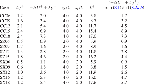

Figure 16. Plots of  ${-\Delta U^{+}}+{{\ell _{U}}^{+}}$ vs ${k}^{+}$, ${\ell _{uv}}^{+}$ and ${({m}{\ell })_e}^{+}$ in ( $a$), ( $b$) and ( $c$), respectively: $\bullet$ (blue), collocated posts (C); ${\blacksquare }$ (red), collocated posts with alternating heights (CC); ${\blacklozenge }$ (green), spanwise-staggered posts (SZ); ${\blacktriangle }$ (magenta), streamwise-staggered posts (SX). —, linear fit $0.78{\ell _{uv}}^{+}$; – – linear fit $0.16{({m}{\ell })_e}^{+}$. Panels (a,b) reproduced using data in Abderrahaman-Elena et al. (Reference Abderrahaman-Elena, Fairhall and García-Mayoral2019). Panel ( $c$) shows ${-\Delta U^{+}}+{{\ell _{U}}^{+}}$ vs their corresponding values of ${{({m}{\ell })}^{+}_e}$ as estimated using (8.2a,b).
Alternatively, one may classify surfaces using appropriate flow quantities instead (Orlandi et al. Reference Orlandi, Leonardi and Antonia2006; Abderrahaman-Elena et al. Reference Abderrahaman-Elena, Fairhall and García-Mayoral2019). The findings of Abderrahaman- Elena et al. (Reference Abderrahaman-Elena, Fairhall and García-Mayoral2019), which are reproduced in figure 16(b), demonstrated that the overall effect of the surfaces in tables 2 and 4 on the turbulent flow are well characterizable using a single flow quantity, namely  ${\ell _{uv}}^{+}$.
Observing the fact that  ${\ell _{uv}}^{+}$ shows a strong linear scaling with respect to ${({m}{\ell })}^{+}$, it is reasonable to assume that the various cases of table 4 should be characterizable in terms of ${({m}{\ell })}^{+}$ while not showing the disparity they do when using $k^{+}$. However, conducting TRM simulations with the aim of reproducing the effects of all these surfaces, as was done in § 6 for the collocated posts (C surfaces), would have entailed a considerable undertaking and fell outside of the scope of this work. Instead, by relying upon a physical intuition of flow over roughness in conjunction with the arguments underlying the TRM boundary conditions, it is examined whether the linear relation between ${-\Delta U^{+}}+{{\ell _{U}}^{+}}$ and ${({m}{\ell })}^{+}$ obtained for the collocated posts can be leveraged for the other surfaces in table 4.
The linear relation between  ${-\Delta U^{+}}+{{\ell _{U}}^{+}}$ and ${({m}{\ell })}^{+}$ obtained for the collocated posts and shown in figure 11(b) is
 \begin{equation} ({-\Delta U^{+}}+{{\ell_{U}}^{+}}) \approx {0.185{{({m}{\ell})}^{+}}+0.36}.\end{equation}
The geometrical differences of the other surface types (table 4) relative to the collocated posts is mainly in terms of their pitch lengths, such that, for a similar height ( $k^{+}$), different levels of drag results. As was argued in § 6.2, the pitch of the posts determines the amount of slip velocity which can arise at the crest plane, and the cross-flow slip plays a role in the occurrence of transpiration. Assuming that, for a given height, the various surfaces translate to a similar transpiration length (i.e. they permit wall-normal momentum to penetrate to approximately the same depth), then the only effect which must be accounted for is the cross-flow slip, which affects transpiration. Hence, the $m^{+}$ contribution of the transpiration factor, ${({m}{\ell })}^{+}$, is assumed to remain fixed, while the ${\ell }^{+}$ component is adjusted
 \begin{equation} {\left ({m}{\ell}\right )}^{+}_e \approx \alpha {{\left ({m}{\ell}\right )}^{+}},\quad \alpha=\frac{{\ell_X}^{+}}{{\ell_C}^{+}}\approx \frac{{\ell_{U,X}}^{+}}{{\ell_{U,C}}^{+}}.\end{equation}
Here,  ${{\ell _{U,X}}^{+}}$ is the mean flow origin (slip velocity) of either the C, CC, SX or SZ surfaces of table 4; ${{\ell _{U,C}}^{+}}$ is the mean flow origin of the collocated posts of table 2 and ${({m}{\ell } )}^{+}_e$ is the expected transpiration factor. As a litmus test for the veracity of the approach undertaken here, the drag estimations obtained from using (8.2a,b) with (8.1) are gathered in table 4 alongside the DNS acquired drag values of Abderrahaman-Elena et al. (Reference Abderrahaman-Elena, Fairhall and García-Mayoral2019). The relative closeness of the estimates to the DNS values substantiates the preceding physical argument which led to (8.2a,b).
Figure 16(c) plots  ${-\Delta U^{+}}+{{\ell _{U}}^{+}}$ of the various surfaces against their corresponding values of ${({m}{\ell })}^{+}_e$. When compared with figure 16(a), it is evident that the transpiration factor serves as a more suitable parameter for characterizing rough surfaces in the transitionally rough regime of turbulence.
The analysis carried out in this section is mainly meant to promote the idea that, for transitionally rough surfaces, effective flow quantities such as  ${\ell }^{+}$ and ${m}^{+}$, which represent the effect of a surface on the flow, may be more suitable for characterizing surfaces in terms of drag rather than surface properties alone, particularly since ${\Delta U^{+}}$ itself is a flow quantity. This could potentially also be exploited for predictive purposes, however, drag prediction of rough surfaces remains an outstanding challenge, even for the fully rough flow regime as detailed in a recent review of the topic by Chung et al. (Reference Chung, Hutchins, Schultz and Flack2021).
9. Conclusions
This work has investigated the TRM, a set of boundary conditions proposed by Lacis et al. (Reference Lacis, Sudhakar, Pasche and Bagheri2020) for modelling the hydrodynamic effect of surface micro-textures on turbulent flows. The occurrence of transpiration is an important physical mechanism of drag-altering surfaces, in particular rough surfaces which cause a drag penalty. The TRM expresses transpiration as being due to the variations in shear of the tangential velocities. This permitted investigating three different conditions for transpiration; only due to streamwise variations ( ${\rm L}\langle \cdot \rangle {\rm MX}\langle \cdot \rangle$), only due to spanwise variations ( ${\rm L}\langle \cdot \rangle {\rm MZ}\langle \cdot \rangle$) and due to variations in both ( ${\rm L}\langle \cdot \rangle {\rm M}\langle \cdot \cdot \rangle$). Coupling to streamwise variations only, while leading to relaxed impermeability, caused no drag increase due to an absence of Reynolds shear stress generation at the boundary plane. Conversely, explicit coupling to spanwise shear variations led to the greatest degree of drag increase due to pronounced turbulent activity taking place at the boundary plane. These simulations reaffirmed that transpiration in wall-bounded canonical turbulence is principally caused by the quasi-streamwise vortices of the near-wall cycle, which to first order induce a spanwise flow.
In terms of surfaces, the effect of small textures would be a displacement of these vortices. This was the effect described by Luchini et al. (Reference Luchini, Manzo and Pozzi1991) for explaining the drag reduction mechanism of riblets. Luchini (Reference Luchini1996) conceptualized this effect as a height difference between imaginary smooth walls perceived by the mean flow and near-wall turbulence with the flow remaining otherwise smooth-wall like. Ibrahim et al. (Reference Ibrahim, Gómez-de-Segura, Chung and García-Mayoral2021) expanded this into a virtual-origin framework for imposing a priori determined virtual origins on the velocities and predicting the resulting drag change. The regime of smooth-wall-like turbulence is also observed for a number of the simulations in this work, with the change in drag being quantified by the difference between the mean flow and turbulence origins expressed by (3.4). Certain conditions identified by Ibrahim et al. (Reference Ibrahim, Gómez-de-Segura, Chung and García-Mayoral2021), which upon violation lead to turbulence ceasing to be smooth-wall like, also remained applicable here. These would be the quasi-streamwise vortices becoming displaced so far downward that they collide with the domain boundary (i.e.  ${{\ell _{uv}}^{+}}\gtrsim 5$) and the near-wall streaks becoming too constricted (i.e. ${\ell _{uv}}^{+}\gtrsim {{{\ell _u}^{+}}+2}$).
The applicability of the TRM in serving as an effective model for rough surfaces in the transitionally rough turbulence regime was also examined. The geometry-resolving transitionally rough DNS data of Abderrahaman-Elena et al. (Reference Abderrahaman-Elena, Fairhall and García-Mayoral2019) were used as references for evaluation. The boundary conditions demonstrate the capability of reproducing the behaviour of the rough surfaces examined up to  $k^{+}\approx 18$, with the flow over the largest roughness sizes falling outside of the regime of smooth-wall-like turbulence. This seems to indicate that such boundary conditions may also cover the flow conditions in the initial region of this non-smooth-like regime. Clearly, this does not apply to situations where the nonlinear interactions between the texture-coherent flow and turbulence become a major component of the near-wall flow dynamics (Abderrahaman-Elena et al. Reference Abderrahaman-Elena, Fairhall and García-Mayoral2019; Fairhall et al. Reference Fairhall, Abderrahaman-Elena and García-Mayoral2019).
A brief examination of TRM derived relations obtained for a specific roughness geometry were leveraged to investigate whether characterizing surfaces in terms of effective flow quantities such as slip and transpiration lengths provide a better means of characterizing roughness in the transitionally rough regime. This was predicated upon the previously observed strong linear relation between the turbulence origin,  $\ell _{uv}^{+}$, and the roughness function, $\Delta U^{+}$, by Abderrahaman-Elena et al. (Reference Abderrahaman-Elena, Fairhall and García-Mayoral2019) for the rough surface geometries they had examined. Unlike measures such as sand-grain roughness height, ${k_s}^{+}$, or effective roughness height, $k^{+}$, which are inadequate in characterizing surfaces in the transitional regime, the transpiration factor, ${({m}{\ell })}^{+}$, is shown to better suit this purpose. Indeed, ${({m}{\ell })}^{+}$ is an indicator of the amount of wall-normal flux that can take place across the crest plane.
For potential future investigations, it is necessary to investigate alternative methods for determining the transpiration coefficients of both regular and irregular rough surfaces. Cost-effective approaches, such as minimal-span channels (Chung et al. Reference Chung, Chan, MacDonald, Hutchins and Ooi2015) or model-based methods (Chavarin & Luhar Reference Chavarin and Luhar2020; Ran, Zare & Jovanović Reference Ran, Zare and Jovanović2021) may prove useful for such purposes. Indeed, it has been shown that the transpiration factor serves the dual purpose of both being an input parameter in the boundary conditions as well as being a metric for characterizing drag. Therefore, once representative values of  $(m\ell )^{+}$ are found, they may be used in CFD applications to investigate more complex geometries. The transpiration lengths obtained in this work by comparing the TRM simulations with geometry-resolving DNS will serve as a reference for developing procedures to determine $m^{+}$ beyond the Stokes regime. Finally, a more extensive formulation of the TRM (Lacis et al. Reference Lacis, Sudhakar, Pasche and Bagheri2020) derived for modelling the effect of porous media on turbulent flows may be similarly investigated. Many of the flow features observed over rough surfaces are also observed over porous structures, such as the linear regime of drag change due to smooth-wall-like turbulence displacement and the existence of a regime exhibiting a Kelvin–Helmholtz-type instability (Jiménez et al. Reference Jiménez, Uhlmann, Pinelli and Kawahara2001; Breugem et al. Reference Breugem, Boersma and Uittenbogaard2006; Manes et al. Reference Manes, Poggi and Ridolfi2011; Kuwata & Suga Reference Kuwata and Suga2017; Gómez-de-Segura & García-Mayoral Reference Gómez-de-Segura and García-Mayoral2019).
Funding
This research was undertaken with the financial support of the Swedish Foundation for Strategic Research (SSF), provided through grant SSF-FFL15-0001. Computational resources were provided by the Swedish National Infrastructure for Computing (SNIC) at the PDC and HPC2N computing centres. The authors also express their gratitude to Dr S. Yogaraj at IIT Goa, for his efforts in developing an earlier implementation of the transpiration boundary condition.
Declaration of interests
The authors report no conflicts of interest.
Appendix A. Numerical solver validation and grid convergence
Figure 17 compares the one-point statistics of the solver used in this work against those of Lee & Moser (Reference Lee and Moser2015), which were obtained using a spectral solver. The agreement between the two datasets is good; with the absolute maximum difference between the mean velocity, r.m.s. velocity fluctuations and Reynolds shear stress not exceeding  $1\,\%$, $2\,\%$ and $1.2\,\%$, respectively. Existing discrepancies are due to the lower effective resolution of second-order finite difference schemes relative to spectral methods at similar grid resolutions as explained by Lee & Moser (Reference Lee and Moser2015).

Figure 17. Mean velocity ( $a$), r.m.s. velocity fluctuation ( $b$) and Reynolds shear stress profiles ( $c$) for a smooth-wall turbulent channel flow: —, solver used in this study; ${\boldsymbol {\circ }}$ (crimson), Lee & Moser (Reference Lee and Moser2015).
For validation of the TRM's Robin boundary conditions; cases L2M0, L5M5 and L10M10 were compared against case DHV220 of Gómez-de-Segura & García-Mayoral (Reference Gómez-de-Segura and García-Mayoral2020) along with cases UWVL2 and UWVL4 of Ibrahim et al. (Reference Ibrahim, Gómez-de-Segura, Chung and García-Mayoral2021). As mentioned in § 3, for isotropic transpiration lengths the wall-normal velocity boundary condition of (2.5) becomes similar to (2.6a–c). Since matching lengths have been used in the boundary conditions of the selected cases, they are equivalent and thus the results should be the same. Unlike the solver used in this study which uses finite differences discretization in all three grid directions, that used by Gómez-de-Segura & García-Mayoral (Reference Gómez-de-Segura and García-Mayoral2020) and Ibrahim et al. (Reference Ibrahim, Gómez-de-Segura, Chung and García-Mayoral2021) employs spectral discretization in the  $x$ and $z$ directions. Nevertheless, as can be seen in figure 18, the data from the simulations are in good agreement, validating the implementation of the boundary conditions.

Figure 18. Comparison of case DHV220,  ${\boldsymbol {\circ }}$ (blue), of Gómez-de-Segura & García-Mayoral (Reference Gómez-de-Segura and García-Mayoral2020) and cases UWVL2, ${\boldsymbol {\square }}$ (green), UWVL4, ${\boldsymbol {\lozenge }}$ (red), of Ibrahim et al. (Reference Ibrahim, Gómez-de-Segura, Chung and García-Mayoral2021) with cases L2M0, — (blue solid line), L5M5, — (green solid line), and L10M10, — (red solid line). The slip and transpiration lengths used in the boundary conditions are listed in table 1 of § 5. The black line represents smooth-wall channel data. Mean velocity $(a)$, r.m.s. velocity fluctuation $(b)$ and Reynolds shear stress $(c)$ profiles.
Figure 19 compares two of the TRM simulations, L2M2 and L2MZ5, with higher resolution counterparts where  $\Delta x^{+} = 4.4$, $\Delta z^{+} = 2.2$, and $0.3\leqslant \Delta y^{+}\leqslant 2.7$ to assess solution grid independence. The mean velocity profiles for both cases do not exceed a $0.6\,\%$ difference in absolute maximum. For the r.m.s. velocity fluctuations; L2M2 and L2MZ5 have absolute maximum differences of approximately $0.2\,\%$ and $0.5\,\%$ respectively for both ${u^{\prime }}_{{rms}}^{+}$ and ${v^{\prime }}_{{rms}}^{+}$, while for ${w^{\prime }}_{{rms}}^{+}$ it is approximately $1\,\%$. The Reynolds shear stress for L2M2 has an absolute maximum difference of approximately $0.3\,\%$, while for L2MZ5 it is $1.4\,\%$. The results demonstrate satisfactory grid independence, with any additional accuracy obtainable by using a higher resolution grid not justifying the increased simulation cost that would result from doing so.

Figure 19. Mean velocity  $(a)$, r.m.s. velocity fluctuation $(b)$ and Reynolds shear stress $(c)$ profiles: — (purple solid line), L2M2, — (green solid line), L2MZ5 with $(N_x, N_y, N_z) = (192, 144, 160)$; — $\!{\square }\!$— (purple), L2M2, — $\!{\lozenge }\!$— (green), L2MZ5 with $(N_x, N_y, N_z) = (256, 252, 256)$.
Appendix B. Cross-analysis with the framework of imposing a priori calculated virtual origins for smooth-wall-like turbulence
The virtual-origin framework has been leveraged in this work to highlight the contributing components to drag modification and identify whether the effect can be solely attributed to that of smooth-wall-like turbulence displacement or alterations of a different nature. It then becomes apt to further compare the results of this work with those of Ibrahim et al. (Reference Ibrahim, Gómez-de-Segura, Chung and García-Mayoral2021) who proposed the framework.
It should first be emphasized that the objective of Ibrahim et al. (Reference Ibrahim, Gómez-de-Segura, Chung and García-Mayoral2021) was prediction of the resulting virtual origins of the different velocity components for a given set of slip-length coefficients,  ${\ell _x}^{+}$, ${\ell _y}^{+}$, ${\ell _z}^{+}$, used in the Robin boundary conditions of (2.6a–c). To do so, they assume that the structure of turbulence remains smooth-wall like and use the r.m.s. velocity profiles of a smooth-wall solution to a priori calculate ${\ell _u}^{+}$, ${\ell _v}^{+}$ and ${\ell _w}^{+}$ using their wall-normal gradients close to the boundary. The calculated origins using smooth-wall data are valid so long as the resulting DNS solutions with the robin boundary conditions fall within the smooth-wall turbulence regime. Within this regime, it also becomes possible to predict the resulting origin for the turbulence, ${y^{+}=-\ell _{uv}}^{+}$, using the origins of ${\ell _w}^{+}$ and ${\ell _v}^{+}$, which quantify the displacement of the quasi-streamwise vortices.
There is a subtle difference between the virtual origins of the velocities,  ${\ell _u}^{+}$, ${\ell _v}^{+}$ and ${\ell _w}^{+}$, and that of the turbulence, ${\ell _{uv}}^{+}$. The latter defines the imaginary smooth wall that the near-wall cycle (essentially the quasi-streamwise vortices) perceives while the former represent the imaginary walls where the velocity components are expected to decay to zero from their values at the boundary plane ( $y^{+}=0$). Hence, while shifting the origin to ${\ell _{uv}}^{+}$ recovers smooth-wall-like turbulence profiles, there would still be some discrepancy in ${u^{\prime }}^{+}$, ${v^{\prime }}^{+}$, ${w^{\prime }}^{+}$ and $-\overline {u^{\prime }v^{\prime }}^{+}$ for the first few layers of $y^{+}$. This is evident in the results of Ibrahim et al. (Reference Ibrahim, Gómez-de-Segura, Chung and García-Mayoral2021) and in the rough-wall simulations of Abderrahaman-Elena et al. (Reference Abderrahaman-Elena, Fairhall and García-Mayoral2019), which remained overall smooth-wall like, with the latter authors observing that ‘Very near the rough surface, different variables would extrapolate to zero at different heights, as is particularly evident for ${u^{\prime }}^{+}$ and ${w^{\prime }}^{+}$ which experience virtual origins shallower than ${\ell _{uv}}^{+}$’ (see figure 13 of the respective paper). This was also pointed out by Ibrahim et al. (Reference Ibrahim, Gómez-de-Segura, Chung and García-Mayoral2021), where they state that ‘The offsets ${\ell _v}^{+}$ and ${\ell _w}^{+}$ are merely prescribed, a priori values to quantify the offset in $v$ and $w$ caused by the surface, but turbulence would react to their combined effect, perceiving a single origin if it is to remain smooth-wall-like’. Additionally, the weakening of permeability to any degree will subject the otherwise viscous-dominated near-wall region to greater perturbations and degrade its laminar-like quality. Hence, a priori determined virtual origins derived from smooth-wall statistics will not be entirely representative of the actual resulting virtual origins of ${u^{\prime }}^{+}$, ${v^{\prime }}^{+}$ and ${w^{\prime }}^{+}$ from DNS where length coefficients have been imposed using boundary conditions for the velocity components, even if the overall turbulence statistics remain smooth-wall like.
The preceding explanations are the reason why, for cases with matching boundary condition coefficients, the a posteriori calculated virtual origins in table 1 differ from the a priori ones of Ibrahim et al. (Reference Ibrahim, Gómez-de-Segura, Chung and García-Mayoral2021). As well be examined further below, this discrepancy does not extend to the origin of the turbulence for matching cases which retain smooth-wall-like turbulence.
For the cases in table 1 involving a transpiration boundary condition, the virtual origin of the turbulence,  ${\ell _{uv}}^{+}$, generally falls in between those of the spanwise and wall-normal velocities, ${\ell _w}^{+}$ and ${\ell _v}^{+}$. This is consistent with the observations made by Gómez-de-Segura et al. (Reference Gómez-de-Segura, Fairhall, MacDonald, Chung and García-Mayoral2018), Gómez-de-Segura & García-Mayoral (Reference Gómez-de-Segura and García-Mayoral2020) and Ibrahim et al. (Reference Ibrahim, Gómez-de-Segura, Chung and García-Mayoral2021). The underlying physical mechanism implied by this was explained in § 3.2.
For drag-reducing cases in which the imposed transpiration length was always smaller than the spanwise slip length ( ${\ell _y}^{+}<{\ell _z}^{+}$), but the predicted origin for $v$ was deeper than $w$ (
$w$ ( ${\ell _v}^{+}>{\ell _w}^{+}$), Ibrahim et al. (Reference Ibrahim, Gómez-de-Segura, Chung and García-Mayoral2021) observed that ${\ell _{uv}}^{+}={\ell _{w}}^{+}$. None of the cases in table 1 have transpiration lengths which are smaller than the slip lengths. The drag neutral case of L2M2 has ${\ell _v}^{+}\approx 2.4$ and ${\ell _w}^{+}\approx 1.7$, but this does not result in ${\ell _{uv}}^{+}={\ell _{w}}^{+}$. Interestingly, case DHV222 of Gómez-de-Segura et al. (Reference Gómez-de-Segura, Fairhall, MacDonald, Chung and García-Mayoral2018) is similar to case L2M2 and the virtual origins reported for it are ${\ell _v}^{+}\approx 2.3$ and ${\ell _w}^{+}\approx 2.0$ ( $1.7$ when curvature is accounted for, as later reported by Gómez-de-Segura & García-Mayoral Reference Gómez-de-Segura and García-Mayoral2020).
To better assess this observed difference, case UWV4 of Ibrahim et al. (Reference Ibrahim, Gómez-de-Segura, Chung and García-Mayoral2021) was replicated. The replicating case is designated L4M2.5 and its raw results were in agreement with that of UWV4 (figure 20). The a posteriori estimated virtual origins for L4M2.5, however, were  ${\ell _u}^{+}\approx 3.2$, ${\ell _w}^{+}\approx 3.0$ and ${\ell _v}^{+}\approx 2.8$, unlike the a priori obtained origins for UWV4 which were ${\ell _u}^{+}\approx 3.6$, ${\ell _w}^{+}\approx 2.9$ and ${\ell _v}^{+}\approx 3.9$. The a posteriori calculated mean flow and turbulence origins for both UWV4 and L4M2.5 are in agreement ( ${\ell _U}^{+}\approx 3.9$, ${\ell _{uv}}^{+}\approx 3.0$ for L4M2.5 and ${\ell _U}^{+}\approx 3.8$, ${\ell _{uv}}^{+}\approx 2.9$ for UWV4 of Ibrahim et al. Reference Ibrahim, Gómez-de-Segura, Chung and García-Mayoral2021), which is to be expected since the simulation results were in agreement.

Figure 20. Comparison of case UWV4,  ${\bullet }$ (blue), of Ibrahim et al. (Reference Ibrahim, Gómez-de-Segura, Chung and García-Mayoral2021) with case L4M2.5, — (red solid line). The slip and transpiration lengths used were ${\ell _x}^{+}={\ell _z}^{+}=4.0$ and ${m_x}^{+}={m_z}^{+}=2.5$. The black line represents smooth-wall data. Mean velocity $(a)$, r.m.s. velocity fluctuations $(b)$ and Reynolds shear stress $(c)$.
Beyond their drag-reducing cases, the virtual-origin framework remained inapplicable to the cases of Ibrahim et al. (Reference Ibrahim, Gómez-de-Segura, Chung and García-Mayoral2021) which demonstrated drag increase as most of them fell outside of the regime smooth-wall-like turbulence. The drag-increasing cases of this work also fall outside of the smooth-wall-like regime. Hence, there are no discrepancies where such cases are concerned.


 Open access