


1. Introduction
The Rayleigh–Taylor (RT) instability occurs at the interface between two superposed fluid layers when the overlying fluid is the more dense and it falls into the lower density fluid under the action of gravity. Given its many applications in nature and in technology (e.g. Sharp Reference Sharp1984; Kull Reference Kull1991), the RT instability has been studied extensively both experimentally (e.g. Lewis Reference Lewis1950; Emmons, Chang & Watson Reference Emmons, Chang and Watson1960; Cole & Tankin Reference Cole and Tankin1973; Fermigier et al. Reference Fermigier, Limat, Wesfreid, Boudinet and Quilliet1992) and theoretically (e.g. Rayleigh Reference Rayleigh1883; Taylor Reference Taylor1950; Chandrasekhar Reference Chandrasekhar1981; Yiantsios & Higgins Reference Yiantsios and Higgins1989; Newhouse & Pozrikidis Reference Newhouse and Pozrikidis1990), with the focus on the case of a thin viscous liquid resting on a horizontal surface or hanging on the underside of a plate. In the equilibrium configuration the interface between the two fluids is flat. A small-amplitude perturbation to this rest state undergoes linear growth followed by the formation of pendant drops (Yiantsios & Higgins Reference Yiantsios and Higgins1989; Elgowainy & Ashgriz Reference Elgowainy and Ashgriz1997) or mushroom-shaped structures (Newhouse & Pozrikidis Reference Newhouse and Pozrikidis1990) in the nonlinear regime. In certain cases the RT instability can be completely suppressed by using an electric field (Taylor & McEwan Reference Taylor and McEwan1965; Tseluiko & Papageorgiou Reference Tseluiko and Papageorgiou2007; Cimpeanu, Papageorgiou & Petropoulos Reference Cimpeanu, Papageorgiou and Petropoulos2014; Anderson et al. Reference Anderson, Cimpeanu, Papageorgiou and Petropoulos2017), a temperature gradient (Kopbosynov & Pukhnachev Reference Kopbosynov and Pukhnachev1986; Burgess et al. Reference Burgess, Juel, McCormick, Swift and Swinney2001) or an insoluble surfactant (Frenkel & Halpern Reference Frenkel and Halpern2017; Kalogirou Reference Kalogirou2018), or through vertical vibrations of the wall (Wolf Reference Wolf1970) or the introduction of wall curvature (Trinh et al. Reference Trinh, Kim, Hammoud, Howell, Chapman and Stone2014). The presence of a shear flow can lead to a nonlinear saturation of the RT instability (Babchin et al. Reference Babchin, Frenkel, Levich and Sivashinsky1983; Frenkel & Halpern Reference Frenkel and Halpern2000; Halpern & Frenkel Reference Halpern and Frenkel2001), in which case the flow can be described by a Kuramoto–Sivashinsky equation (Hooper & Grimshaw Reference Hooper and Grimshaw1985).
In this work we consider the RT instability that emerges at the interface between two immiscible viscous fluids in a horizontal channel which are undergoing shear flow due to the horizontal translation of the upper channel wall. Inertia is neglected so that instability due to viscosity stratification does not occur (Yih Reference Yih1967). This system is susceptible to the early-stage linear growth alluded to above and a formal linear stability analysis demonstrates that small-amplitude wave-like disturbances are unstable if their wavenumber lies in a range that is subtended between zero and a finite cut-off value (assuming non-zero interfacial tension) (Chandrasekhar Reference Chandrasekhar1981). Thus the instability is essentially long-wave in character and with this in mind we focus our attention on long-wave perturbations. In particular we study the dynamics mainly via a nonlinear evolution equation that we derive and which includes the effects of surface tension, viscosity stratification and gravity, but ignores inertia.
Interestingly, even though related lubrication equations have been obtained by several other authors (Hammond Reference Hammond1983; Yiantsios & Higgins Reference Yiantsios and Higgins1989; Oron, Davis & Bankoff Reference Oron, Davis and Bankoff1997; Bertozzi & Pugh Reference Bertozzi and Pugh1998; Jensen Reference Jensen2000; Lister et al. Reference Lister, Rallison, King, Cummings and Jensen2006; Tseluiko & Papageorgiou Reference Tseluiko and Papageorgiou2007), investigations of the validity of such equations through comparisons with experimental data or direct numerical simulations (DNS) have been limited. Anderson et al. (Reference Anderson, Cimpeanu, Papageorgiou and Petropoulos2017) obtained a non-local equation describing the evolution of an electrified viscous thin film wetting the underside of a wall, and carried out DNS to assess the accuracy of the asymptotic model. In this work we also perform DNS, and attempt qualitative comparisons to examine the validity of our numerical results based on the lubrication equation, even for parameter sets outside the applicability region of the model.
A key parameter in our problem is the Bond number, which acts as a measure of the relative strength of gravitational and surface tension forces. In our case adverse density stratification is in place for any positive value of the Bond number, leading to RT instability and the appearance of large-amplitude protrusions at the fluid–fluid interface. As we shall see, these protrusions initially take the form of individual fingers that travel in the same direction as the basic shear flow. The emergence of such fingers is of course common in RT phenomena; what is of particular interest here is the way in which these fingers are advected with the flow and interact with one another. In fact we see in our simulations that a coarsening of the dynamics occurs as the fingers run into one another, following a sequence of merging events that leads ultimately to the formation of a residual, solitary finger which propagates with a very nearly fixed form and at a near-constant speed. When the Bond number is sufficiently large, this solitary wave spans the whole of the channel height and, in so doing, effectively (almost) segregates the two fluids. We also establish that the interface may not achieve touch-down or touch-up at the channel walls in finite time. We note that singularity formation has been investigated analytically in related thin-film flow studies (e.g. Bertozzi & Pugh Reference Bertozzi and Pugh1998; Tseluiko & Papageorgiou Reference Tseluiko and Papageorgiou2007), where uniform boundedness of solutions has been rigorously established.
In § 2 we introduce the governing equations and present the lubrication model partial differential equation (the derivation is provided in an appendix). In § 3 we present and discuss the results of unsteady numerical simulations of the model equation (§ 3.1) to reveal the coarsening dynamics mentioned above and the eventual emergence of fixed-form travelling-wave solutions. The latter are investigated using a continuation method in § 3.3, and the results are compared with those obtained from DNS of the full Stokes equations in § 3.4. Further insight into the shape of the final travelling-wave state is attained in § 4 via a large-Bond-number asymptotic analysis that also reveals a simple leading-order formula for the wave speed which depends only on the viscosity stratification parameter. In § 5 we summarise our findings.
2. Mathematical model
We consider an unstably stratified two-fluid flow in a horizontal channel of fixed height  $d$, with the top fluid (labelled as fluid 2) being heavier than the bottom fluid (labelled as fluid 1) such that the fluid densities satisfy $\rho _2>\rho _1$. The two fluids have generally different viscosities $\mu _1\ne \mu _2$, and the flow in the channel is driven by the horizontal motion of the upper channel wall with speed $U$. The problem is expressed in non-dimensional form by rescaling lengths with $d$, velocities with $U$, pressures with $\mu _1U/d$ and time with $d/U$. We neglect fluid inertia and study the dynamics under the conditions of Stokes flow.
We define a Cartesian coordinate system, with  $x$ being the horizontal coordinate, $y$ the vertical coordinate and $t$ denoting time. In non-dimensional terms, the channel walls are at $y=0$ and $y=1$ and the fluids are separated by an interface at $y=h(x,t)$. Defining the velocity vector $\boldsymbol {u}_j=(u_j,v_j)$ in each fluid ( $j=1,2$), where the velocity components are space- and time-dependent, the dynamics within each fluid layer is governed by the non-dimensional continuity and Stokes equations:
 \begin{equation} \boldsymbol{\nabla} \boldsymbol{\cdot} \boldsymbol{u}_j = 0, \quad 0 ={-}\boldsymbol{\nabla} p_j + m_j\nabla^2\boldsymbol{u}_j - \frac{r_j}{(r-1)}\frac{B}{C}\boldsymbol{\hat{y}}, \end{equation}
where  $p_j=p_j(x,y,t)$ is the fluid pressure, $\boldsymbol {\nabla }=(\partial _x,\partial _y)$ is the gradient operator and ${\hat {\boldsymbol {y}}=(0,1)^{\rm T}}$ is the unit vector that points in the opposite direction to the gravitational force. The parameters $m_1=1$, $m_2=m$, $r_1=1$ and $r_2=r$, where $m=\mu _2/\mu _1$ and
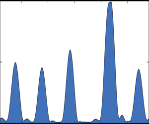
  $r=\rho _2/\rho _1$ are the viscosity ratio and the density ratio, respectively. The capillary number, $C$, and the Bond number, $B$, are defined by
 \begin{equation} C = \frac{\mu_1U}{\gamma} > 0, \quad B = \frac{(\rho_2-\rho_1)gd^2}{\gamma} = (r-1)\frac{\rho_1gd^2}{\gamma} > 0, \end{equation}
where  $\gamma$ is the interfacial tension and $g$ is the acceleration due to gravity. The boundary conditions at the channel walls and at the interface are
 \begin{align}& \boldsymbol{u}_1=(0,0) \quad\text{at}\ y=0; \quad \boldsymbol{u}_2=(1,0) \quad\text{at}\ y=1; \end{align}
 \begin{align}& \boldsymbol{u}_1 = \boldsymbol{u}_2, \quad \left[(\boldsymbol{n}\boldsymbol{\cdot}\boldsymbol{\sigma}_j)\boldsymbol{\cdot} \boldsymbol{n}\right]_2^1 = C^{{-}1}\kappa, \quad \left[(\boldsymbol{n}\boldsymbol{\cdot}\boldsymbol{\sigma}_j)\boldsymbol{\cdot} \boldsymbol{t} \right]_2^1 = 0 \quad\text{at}\ y=h(x,t), \end{align}
where the jump notation  $[f_j]_2^1=f_1-f_2$ is used. The last two equations in (2.3b) are the interfacial normal and tangential stress jumps, respectively, where $\boldsymbol {\sigma }_j$ is the (dimensionless) stress tensor in fluid $j$, defined by
 \begin{equation} \boldsymbol{\sigma}_j ={-}p_j\boldsymbol{I} + \left( \boldsymbol{\nabla}\boldsymbol{u} + (\boldsymbol{\nabla}\boldsymbol{u})^{\rm T} \right), \quad j=1,2, \end{equation}
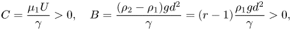
and  $\boldsymbol {I}$ is the identity matrix. The unit normal vector $\boldsymbol {n}$ at the interface (pointing into the lower fluid), the unit tangent vector $\boldsymbol {t}$ at the interface and the interfacial curvature $\kappa$ are given by
 \begin{equation} \boldsymbol{n} = \frac{(h_x, -1)}{(1+h_x^2)^{1/2}}, \quad \boldsymbol{t} = \frac{(1,h_x)}{(1+h_x^2)^{1/2}}, \quad \kappa = \frac{h_{xx}}{(1+h_x^2)^{3/2}}. \end{equation}
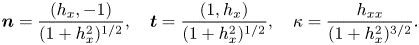
Following Ooms, Segal & Cheung (Reference Ooms, Segal and Cheung1985), we impose the constraint that the total flow rate through the channel,
 \begin{equation} Q(t) = \int_0^{h(x,t)} u_1(x,y,t)\,{\mathrm d} y + \int_{h(x,t)}^1 u_2(x,y,t)\,{\mathrm d} y, \end{equation}
is fixed at time  $t$ so that there is no pressure drop over a domain of specified length in the $x$ direction.
The unstably stratified system is characterised by the appearance of long waves at the interface (Yiantsios & Higgins Reference Yiantsios and Higgins1989). Consequently, exploiting the disparity between the  $x$ and $y$ length scales, we perform a lubrication analysis to derive the following model system that will allow us to study the nonlinear spatio-temporal interfacial dynamics (see Appendix A for a detailed derivation):
 \begin{equation} h_t + q_x = 0,\quad{\rm with}\ q = \mathscr{D}^{{-}1}\left( mh^2H_1 + \frac{1}{3}h^3(1-h)^3H_2\mathcal{F} \right), \end{equation}
where  $\mathscr {D}$, $H_1$, $H_2$, $\mathcal {F}$ are all functions of $h$ and are defined by
 \begin{align} \mathscr{D}(h) &= m^2h^4 + 2mh(1-h)\Big(2-h(1-h)\Big) + (1-h)^4 > 0, \end{align}
 \begin{align}H_1(h) &= (m-1)h^3 + (Q-1)(m-1)h^2 + (1-2Q)h + (3Q-1), \end{align}
 \begin{align}H_2(h) &= (1-h)+mh > 0, \end{align}
 \begin{align}\mathcal{F}(h) &= C^{{-}1}(Bh_x + h_{xxx}). \end{align}
The functions  $\mathscr {D}$ and $H_2$ are positive provided that $0< h<1$, while the functions $H_1$ and $\mathcal {F}$ can each be of either sign depending on the values of $Q(t)$, $h_x$ and $h_{xxx}$. The lubrication model presented above is similar to the model of Tilley, Davis & Bankoff (Reference Tilley, Davis and Bankoff1994) and it reduces to those obtained in related studies on channel flows with surfactant (Blyth & Pozrikidis Reference Blyth and Pozrikidis2004; Frenkel & Halpern Reference Frenkel and Halpern2017; Kalogirou & Blyth Reference Kalogirou and Blyth2020), in the case when surfactant is neglected.
Small-amplitude long-wave disturbances are unstable according to (2.7) as is expected in the presence of adverse density stratification,  $B>0$, when gravity has a destabilising effect (Oron et al. Reference Oron, Davis and Bankoff1997). Of particular interest here is the character of the nonlinear wave development as the interfacial amplitude grows beyond the confines of the linear regime. To this end, in the next section we focus on carrying out numerical simulations of the evolution equation (2.7) in a domain that is sufficiently large, to capture the instability due to density stratification.
3. Numerical results
3.1. Time-dependent simulations of the lubrication equation (2.7)
The lubrication equation (2.7) is solved numerically using a pseudospectral scheme (e.g. Trefethen Reference Trefethen2000) on a periodic domain  $[-L,L]$ and the unconditionally stable Crank–Nicolson method is used for the time discretisation. The discretised nonlinear system is solved at each time level by using Newton's method. The (unknown) flow rate $Q(t)$ is calculated at each time step by imposing the zero-pressure-drop condition (A12), which is done numerically by setting the integral of the pressure gradient (A11) to zero and solving for $Q(t)$ (integrals are approximated by the trapezoidal rule). In all the simulations presented in this work, the (half) domain length is fixed to $L=28$, which is sufficiently large to capture the phenomena of interest. Typically, $512$ grid points are used to discretise the spatial domain, so the grid resolution is $2L/512=0.0194$, and a time step of size $0.05$ is found to be sufficient to produce accurate results.
The initial condition corresponds to a sinusoidal disturbance superimposed on a flat interface at uniform height  $h_0$, and is given by
 \begin{equation} h(x,0) = h_0\left[ 1 + h_A \cos\left(\frac{n{\rm \pi} x}{L}\right) \right], \end{equation}
where  $h_A$ is a constant and $n$ is an integer. In what follows we describe the dynamics for the particular case $h_A=0.2$ and $n=1$. Following extensive simulations with other choices of these parameters (some further comment on which is provided below), including combinations of Fourier modes and amplitudes $h_A$ selected from a random distribution, this was found to be representative of the dynamics that is observed. Unless otherwise stated, the parameters used in the numerical computations are $h_0=0.2$, $m=0.5$, $C=10^{-3}$ and $B=1$.
Interfacial profiles at different stages of the simulation starting from the initial condition (3.1) and using the aforementioned parameter set are shown in figure 1. At early times a number of protrusions, hereinafter referred to as fingers, appear on the interface. In this case six fingers emerge, as can be seen in figure 1(a–c) corresponding to  $t=15,20,35$. Intuition suggests that the number of fingers will be dependent on the size of the Bond number, since a greater density disparity between the two fluids should correspond to a greater susceptibility to interfacial instability. While in the present results it takes approximately 35 time units for all six fingers to clearly form at the interface, we note that for larger values of $B$ more fingers develop and also these emerge earlier in the simulation.

Figure 1. Interfacial profiles obtained at different times (a)  $t=15$, (b) $t=20$, (c) $t=35$, (d) $t=50$, (e) $t=100$ and ( f) $t=200$ for the parameter values $h_0=0.2$, $m=0.5$, $C=10^{-3}$ and $B=1$. Starting from an initial condition of the form (3.1) with $h_A=0.2$ and $n=1$ (also shown with a broken line in panel a), six distinct fingers are seen to develop at early times in the simulation. These then get closer to the lower wall and slowly drift to the right due to background shear flow. The tallest finger travels faster and eventually merges with the finger directly in front of it. The merging dynamics continues to take place until a single wide finger remains that almost touches both channel walls. The solution seen in ( f) has been shifted to the right by a distance $L=28$ for better visualisation of the final finger. The time evolution of the interfacial profile can be seen in the supplementary movie available at https://doi.org/10.1017/jfm.2022.1070.
The number of fingers formed can be estimated using the growth rates determined from linear theory (e.g. Tseluiko & Papageorgiou Reference Tseluiko and Papageorgiou2007). These are calculated from (2.7) by writing  $h=h_0+A\exp (\mathrm {i} Kx+\sigma t)+ \text {c.c.}$ (complex conjugate), and linearising on the basis that $A/h_0\ll 1$ with a view to calculating $\sigma$ for a prescribed wavenumber $K$ (more details are provided in Appendix B). In figure 2, the linear growth rate, $\mathrm {Re}(\sigma )$, is plotted against the spatial frequency $k = L K /{\rm \pi}$ for various values of the Bond number $B$. In the context of the numerical simulations of the evolution equation (2.7), the variable $k$ is taken to be an integer corresponding to the number of wavelengths that fit exactly into the computational domain of length $2L$. The fastest growing mode in the numerical simulation corresponds to the spatial frequency closest to that which maximises the growth rate, namely $k_{max} = (L/{\rm \pi} )\sqrt {B/2}$ (see Appendix B). For example, when $L=28$ we have $k_{max}\approx 6$ for $B=1$ and $k_{max}\approx 9$ for $B=2$, the former prediction being in line with the six fingers that are observed in figure 1(c). The cut-off wavenumber for linear instability is $K_c=\sqrt {B}$ so that the range of unstable wavenumbers depends solely on the Bond number (see also Oron et al. Reference Oron, Davis and Bankoff1997). Accordingly, in the simulations we must choose integer $k< LK_c/{\rm \pi}$ in order to observe instability.
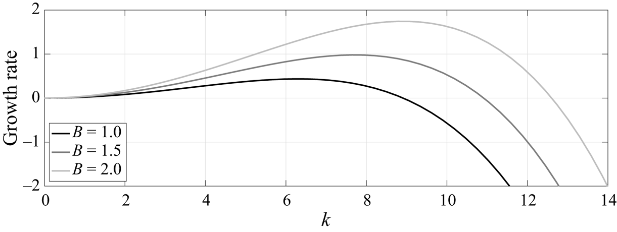
Figure 2. Linear growth rate for different values of the Bond number, plotted against  $k=({L}/{{\rm \pi} })K$, where $K$ is the wavenumber and $L=28$ is the (half) domain length. Parameter values for $h_0$, $m$,
$m$,  $C$ are the same as in figure 1. A positive growth rate is supported for wavenumbers in the range $K\in (0,\sqrt {B})$, so interfacial instability is enhanced as the value of $B$ increases. The maximum growth rate occurs at $k_{{max}}=(L/{\rm \pi} )\sqrt {B/2}$.
Finger formation similar to that seen in figure 1 has also been observed in a related study of channel flow by Mavromoustaki, Matar & Craster (Reference Mavromoustaki, Matar and Craster2010). In the absence of the shear flow (so when the upper wall is stationary), the finger pattern in the interfacial profile retains the symmetry of the initial condition (3.1) approximately  $x=0$ (see related studies on static liquid film configurations, for example those by Yiantsios & Higgins (Reference Yiantsios and Higgins1989), Bertozzi & Pugh (Reference Bertozzi and Pugh1998), Tseluiko & Papageorgiou (Reference Tseluiko and Papageorgiou2007), Wang, Mählmann & Papageorgiou (Reference Wang, Mählmann and Papageorgiou2009), Barannyk et al. (Reference Barannyk, Papageorgiou, Petropoulos and Vanden-Broeck2015) and Wang & Papageorgiou (Reference Wang and Papageorgiou2018)). Here the symmetry is broken by the superimposed shear flow and consequently the interfacial profile tends to drift in the positive $x$ direction. The individual fingers (as seen in the various panels of figure 1) travel more or less holding their shape, size and speed. Generally speaking, taller fingers have greater volume and move faster, as is confirmed in § 3.3. As a result the tallest finger eventually catches up with the finger directly in front of it, and the pair subsequently merge to form a larger finger whose volume is approximately the sum of the two individual volumes. An example can be seen in figure 1(c,d), where the interfacial profiles are displayed at $t=35,50$. After this first coalescence, the tallest finger has gained sufficient volume to approach the upper channel wall (see figure 1d). The merging process continues so that the number of fingers gradually diminishes until only a single, rather wide, finger remains (see figure 1f); this finger essentially combines the individual volumes of all fingers from the earlier stage of the simulation, with any deficit accounted for in the thin lower fluid film that comprises the remainder of the flow domain. Note that despite the apparently rather steep slope on either side of the finger, the scales are such that the gradient here is modest, so that the legitimacy of the assumed lubrication approximation ought to be maintained. With reference to alternative choices of initial condition mentioned above, broadly similar dynamics is observed, including the occurrence of merging events, the only difference being the number of final-state fingers (akin to that at $t=200$ in figure 1) that are ultimately obtained. Similar coarsening dynamics has been reported by Glasner & Witelski (Reference Glasner and Witelski2003) and Kitavtsev (Reference Kitavtsev2014) who investigated dewetting of thin films, as well as by Chang, Demekhin & Kalaidin (Reference Chang, Demekhin and Kalaidin2000) and Razis et al. (Reference Razis, Edwards, Gray and van der Weele2014) in their studies of roll wave structures propagating down an inclined plane.
The merging events just described can also be seen in the evolution of the displacement norm  $\|h-h_0\|_2$ shown in figure 3(a), where each of the sudden upward steps in the curve corresponds to the merging of a pair of fingers. The final merging event occurs at around $t=150$ when the norm reaches the final plateau, and after this time the solitary finger propagates downstream essentially retaining the same form for the remainder of the simulation. Also shown in figure 3 is the trace of the interfacial minimum and maximum during the simulation. The minimum first decreases until around $t=35$ when the interface almost makes contact with the bottom wall; at the same time the maximum increases until the interface almost touches the upper wall (this occurs at around $t=50$; see also figure 1c,d). At later times the interfacial minimum and maximum settle down to a near-constant value; in fact they exhibit small-amplitude and apparently random fluctuations approximately a mean level, as can be seen from figure 3(d,e). This irregular large-time behaviour is reminiscent of the chaotic dynamics seen in the evolution of thin films (e.g. Kawahara Reference Kawahara1983; Kawahara & Toh Reference Kawahara and Toh1988; Kalogirou & Papageorgiou Reference Kalogirou and Papageorgiou2016). We explain this by noting that at large times the near-saturated state features a thin film of the lower fluid over much of the domain, and a thin film of the upper fluid confined between the top of the finger and the upper wall. The evolution of these thin films can be described by Kuramoto–Sivashinsky-type equations (see Appendix C and the related studies by Hooper & Grimshaw (Reference Hooper and Grimshaw1985), Charru & Fabre (Reference Charru and Fabre1994), Tilley et al. (Reference Tilley, Davis and Bankoff1994) and Kalogirou et al. (Reference Kalogirou, Cimpeanu, Keaveny and Papageorgiou2016)), which are well known for demonstrating chaotic behaviour (Papageorgiou, Maldarelli & Rumschitzki Reference Papageorgiou, Maldarelli and Rumschitzki1990). Both films are linearly unstable with a growth rate of the order of $10^{-3}$; its small size is attributable to the $h_0^3$ and $(1-h_0)^3$ terms in the growth rate formula (B2). In related studies where the flow evolves from a static initial state, the fluid film tends to approach the wall in infinite time (Tseluiko & Papageorgiou Reference Tseluiko and Papageorgiou2007). Such a touch-down scenario appears to be absent here, and we believe the near saturation combined with thin-gap chaotic dynamics is connected with the background shear flow. In Appendix D we provide an analytical argument to support the numerical results seen in figures 1 and 3, in particular that the solution remains bounded such that $0< h<1$ for all time.
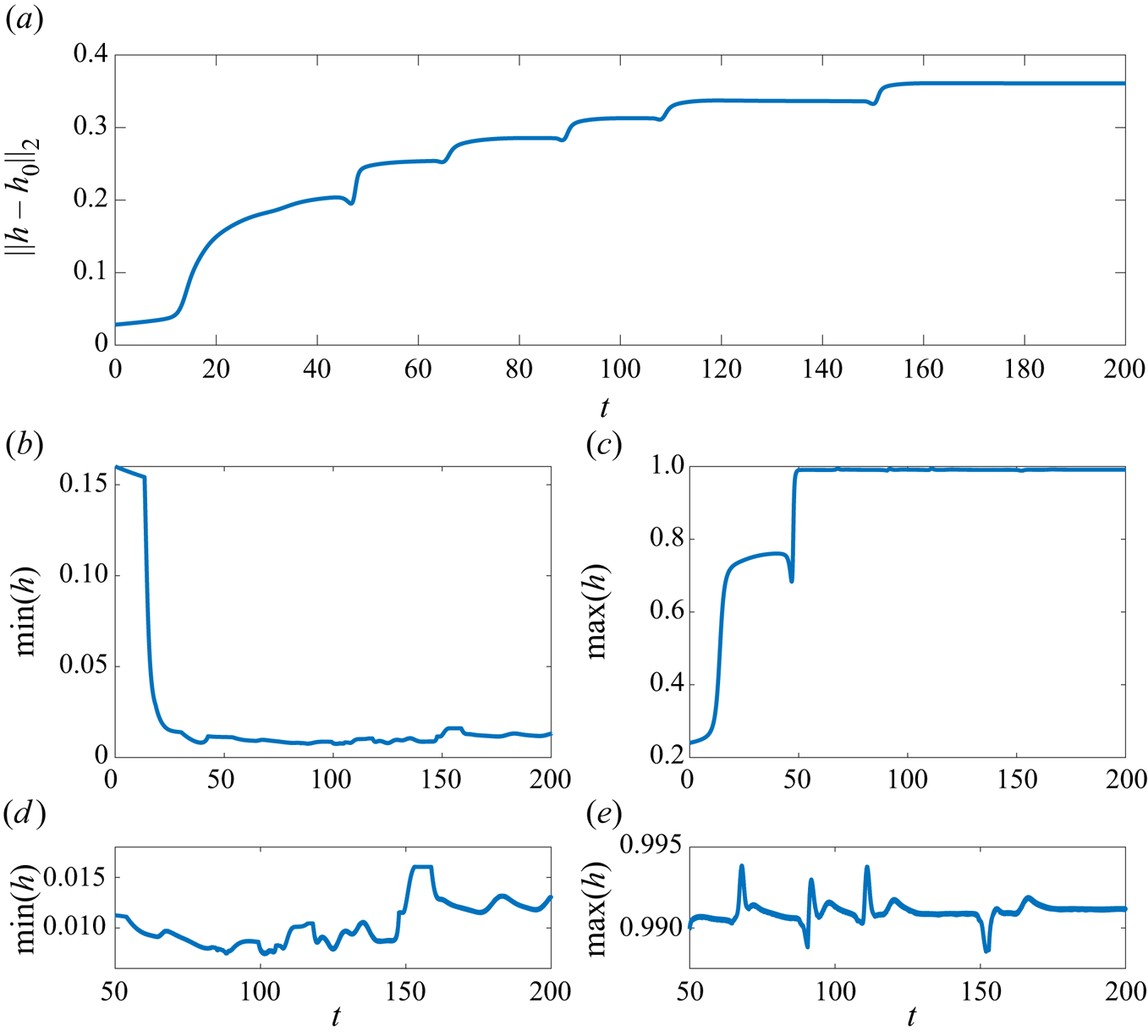
Figure 3. (a) Time evolution of interfacial solution norm, (b,c) interfacial minimum and maximum, including (d,e) a close-up evolution at later times of the simulation. Parameter values for  $h_0$, $m$,
$m$,  $C$,
$C$,  $B$ remain the same as in figure 1.
The final interfacial wave profile in figure 1( f), also shown in figure 4(a), features a capillary ridge and a depression on the top-right and the bottom-right part of the finger, respectively (these features are more obviously seen in the sketch in figure 11; see also in figure 13b). The interfacial velocity, shown with a red thin line in figure 4(a), becomes large in magnitude at the two points  $x_1$ and $x_2$ where the interface is closest to each wall (similar behaviour was observed in Papageorgiou, Petropoulos & Vanden-Broeck (Reference Papageorgiou, Petropoulos and Vanden-Broeck2005), Wang et al. (Reference Wang, Mählmann and Papageorgiou2009) and Barannyk et al. (Reference Barannyk, Papageorgiou, Petropoulos and Vanden-Broeck2015)). To understand the source of these peaks we plotted the magnitude of the various terms that define the interfacial velocity in (A8) to determine which term dominates. We found that the $\mathcal {F}$ term, defined in (2.8d), experiences (positive or negative) peaks as can be seen in figure 4(b), but these are most pronounced where the interface is closest to each wall (i.e. at the points labelled as $x_1$ and $x_2$). We note that the $\mathcal {F}$ term is related to $F_\chi$ in (A7b) and that this term dominates over the other terms in the pressure gradient expression (A11). The large negative peaks in the profile of $\mathcal {F}$ lead to large negative spikes in pressure gradient, which drives the rapid flow near the walls (note that the flat parts of the $\mathcal {F}$ curve are much smaller in magnitude, on the scale shown, but not constant).
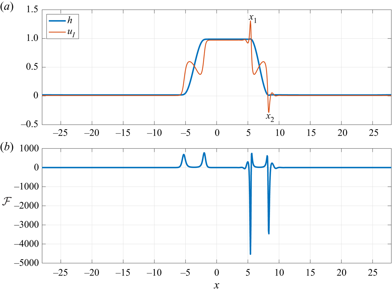
Figure 4. (a) Profile  $h$ of the interfacial wave (blue line) and interfacial horizontal velocity $u_I=u|_{y=h}$ (red line) and (b) term $\mathcal {F}=C^{-1}(Bh_x + h_{xxx})$ which dominates in the pressure gradient distribution, plotted at time $t=200$. Parameter values for $h_0$, $m$,
$m$,  $C$,
$C$,  $B$ are the same as in figure 1. The interfacial velocity is seen to become large in magnitude at the two points $x_1$ and $x_2$ where the interface takes the form of a capillary ridge or depression and is closest to the upper/lower channel walls. This is accompanied by a drop in the pressure gradient as evident by the dips in the profile of term $\mathcal {F}$.
3.2. Physical discussion
Intuition might suggest that the action of gravity will lead to the heavier fluid displacing the lower, lighter fluid. In a static configuration for which there is no preference for flow to the right or left, one would anticipate that a localised interfacial disturbance will tend to migrate upwards as fluid is drawn in from either side by hydrostatic force. Since the shear flow removes the left/right symmetry, the possibility arises of a finite-amplitude travelling wave that is sustained by a tripartite combination of shear, gravity and surface tension. Indeed, this has been demonstrated in the weakly nonlinear regime by Babchin et al. (Reference Babchin, Frenkel, Levich and Sivashinsky1983). Examples of fully nonlinear waves in related unstably stratified problems include travelling waves on fluid films flowing down the underside of an inclined plane – see, for example, Kofman et al. (Reference Kofman, Rohlfs, Gallaire, Scheid and Ruyer-Quil2018) and Zhou & Prosperetti (Reference Zhou and Prosperetti2022).
Considering moderate- to large-amplitude waves, we now examine more closely one of the travelling-wave solutions obtained as the large time limit of the initial value problem for the lubrication model equation (2.7) solved in § 3. In figure 5 we show the final-state interfacial profile when  $B=0.1$ together with the corresponding streamline pattern in a frame of reference that is travelling at the wave speed. Figure 6 shows a more highly deformed interfacial profile computed for $B=0.4$. We note the striking qualitative similarity between the interfacial profile seen in figure 5 and that computed for a viscous film flowing on the underside of an inclined plate (see e.g. Kofman et al. Reference Kofman, Rohlfs, Gallaire, Scheid and Ruyer-Quil2018; Zhou & Prosperetti Reference Zhou and Prosperetti2022).

Figure 5. (a) Flow configuration and (b) interfacial curvature for  $B=0.1$ and parameters $h_0$, $m$,
$m$,  $C$ fixed to the same values as in figure 1. In (a), the colour corresponds to the vertical velocity $v_1$ in the lower fluid, the thick line indicates the location of the interface and thin lines shown within the fluids are the streamlines.
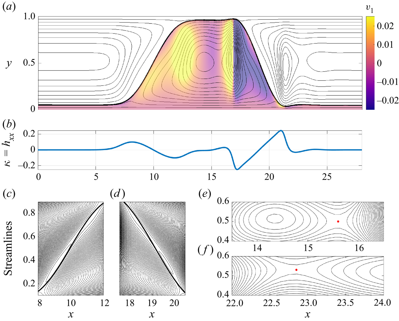
Figure 6. (a) Flow configuration and (b) interfacial curvature for  $B=0.4$ and parameters $h_0$, $m$,
$m$,  $C$ fixed to the same values as in figure 1. The colour in (a) corresponds to the vertical velocity $v_1$ in the lower fluid. In (a,c–f), the thick line indicates the location of the interface and the thin lines shown within the fluids are the streamlines. Two clockwise-moving eddies exist in each fluid (panel a), and the streamlines are seen to cross at two stagnation points at $(x,y)=(15.6,0.5)$ and $(22.85,0.53)$, indicated by red dots in (e, f). Near the transition regions where the interface ascends/descends from one wall to the other, a total of four smaller counterclockwise-moving eddies are generated due to the draught from the surrounding fluids, as shown in (c,d).
The speed of the travelling frame is 0.18 for figure 5 and 0.465 for figure 6, both of which values are smaller than the upper wall speed, which is unity according to our non-dimensionalisation. Consequently, in both figures the flow is from right to left in the lower part of the channel and from left to right in the upper part of the channel. Focusing on the results in figure 5, located in the main part of the upward bulge in the lower fluid is an eddy with fluid circulating in the clockwise direction. Critically, the interface is not symmetric about the vertical line through the eddy centre. The fluid is drawn upward on the left-hand side of the eddy by hydrostatic force. On the right-hand side of the eddy the large curvatures that occur around  $x=-2.5$ and $x=5$ suggest that the capillary force is sufficiently strong to combat the hydrostatic effect and to drive the fluid downwards. The whole structure is sustained by the background shear flow which flushes the rest of the lower fluid away to the left.
For fairly small Bond number, the effect of surface tension is relatively strong and only reasonably mild interfacial curvature is needed to provide the necessary capillary pressure to support the eddy motion. For larger Bond number the relative effect of surface tension is weaker and much larger curvatures are needed to provide the necessary capillary pressure. Thus we see the notably sharper features in the interfacial profile for  $B=0.4$ in figure 6 at approximately $x=17$ and $x=21$, and the much stronger curvatures at the same locations, roughly a factor of ten larger than the corresponding values for the $B=0.1$ case. Interestingly, the flow structure is more complex for the larger Bond number. There are many stagnation points within a single flow period: eight are located at the centre of eddies (note the four very slender eddies adjacent to the interface, which can be seen in figure 6c,d), two more are located at local saddle points in the streamline pattern evident in figure 6(e,f) and several others are located on the interface itself.
3.3. Travelling-wave solutions
The results of the numerical simulation discussed in the previous section indicated that the interface evolves into a travelling wave. Although the flow was found to be chaotic in the narrow gaps at the walls, this does not significantly affect the rest of the wave profile so that overall the interfacial travelling wave propagates with approximately fixed form and constant speed in the direction of the background shear flow. Motivated by this, in this section we seek travelling-wave solutions to the evolution equation (2.7) using the continuation software AUTO-07p (Doedel & Oldman Reference Doedel and Oldman2009). Introducing the travelling-wave coordinate  $\xi =x-ct$, with wave speed $c>0$, equation (2.7) becomes
 \begin{equation} - ch_\xi + q_\xi = 0. \end{equation}
Assuming steady flow in the travelling-wave frame, we take the total flow rate  $Q$ to be constant.
To prepare the ground for the computations in AUTO, we define the scaled independent variable  $X=(\xi +L)/(2L)$, so that $X\in [0,1]$, and rewrite (3.2) as the first-order system of ordinary differential equations $\boldsymbol {U}_X = 2L\mathcal {A}(\boldsymbol {U})$, where
 \begin{align} \boldsymbol{U} \equiv (U_1, U_2, U_3, U_4) \equiv (h, h_X, h_{XX}, h_{XXX}) \quad \text{and} \quad \mathcal{A}(\boldsymbol{U}) \equiv \left(U_2, U_3, U_4, \mathcal{N}(\boldsymbol{U})\right). \end{align}
The nonlinear function  $\mathcal {N}(\boldsymbol {U})$ in (3.3a,b) is found by rearranging equation (3.2) for $h_{XXXX}$; see also the expression for $q$ in (2.7b) and the definition of $\mathcal {F}$ in (2.8d). Periodic boundary conditions are imposed on $h, h_X, h_{XX}$. Three integral constraints are imposed to fix the volume of each fluid in a domain period, to break the translational invariance of the system (Sandstede Reference Sandstede2002; Champneys & Sandstede Reference Champneys and Sandstede2007) and to enforce the zero-pressure-drop condition (A12). The parameter continuation is initiated close to the bifurcation point for small-amplitude periodic waves using the approximate solution $h(X) = h_0 + 10^{-3}\cos (2{\rm \pi} X)$. The remaining parameters are determined so that the initial guess is close to neutral stability, according to predictions from linear theory (see Appendix B).
The number of free parameters in the continuation is determined by the relation  $N_{cont}=N_{bc}+N_{int}-N_{dim}+1$, where $N_{bc}$ is the number of boundary conditions, $N_{int}$ is the number of integral constraints and $N_{dim}$ is the size of the system (Doedel & Oldman Reference Doedel and Oldman2009). Here we have $N_{bc}=N_{int}=3$ and $N_{dim}=4$ (cf. (3.3a,b)), and hence $N_{cont}=3$. We perform continuation in terms of the travelling-wave speed $c$, the flow rate $Q$ and one other geometrical or physical parameter, such as the (half) domain length $L$ or the undisturbed lower fluid thickness $h_0$, while holding the rest of the parameters fixed.
Interfacial wave profiles obtained for different values of  $B$ are shown in figure 7 (the parameters $h_0$, $m$ and $C$ are set to the same values as in the previous section). Evidently the interface forms an increasingly pronounced finger as the Bond number increases. This results in a near segregation of the two fluids as the finger almost touches the walls at sufficiently large $B$. This is consistent with the time-dependent calculations of the previous section. In fact the profile for $B=1$ is almost identical to the final wave state in figure 1(f), the only difference being that the thin-film regions near each wall are in the present case flat and steady. The capillary ridge and the depression at the leading edge of the finger are also apparent.
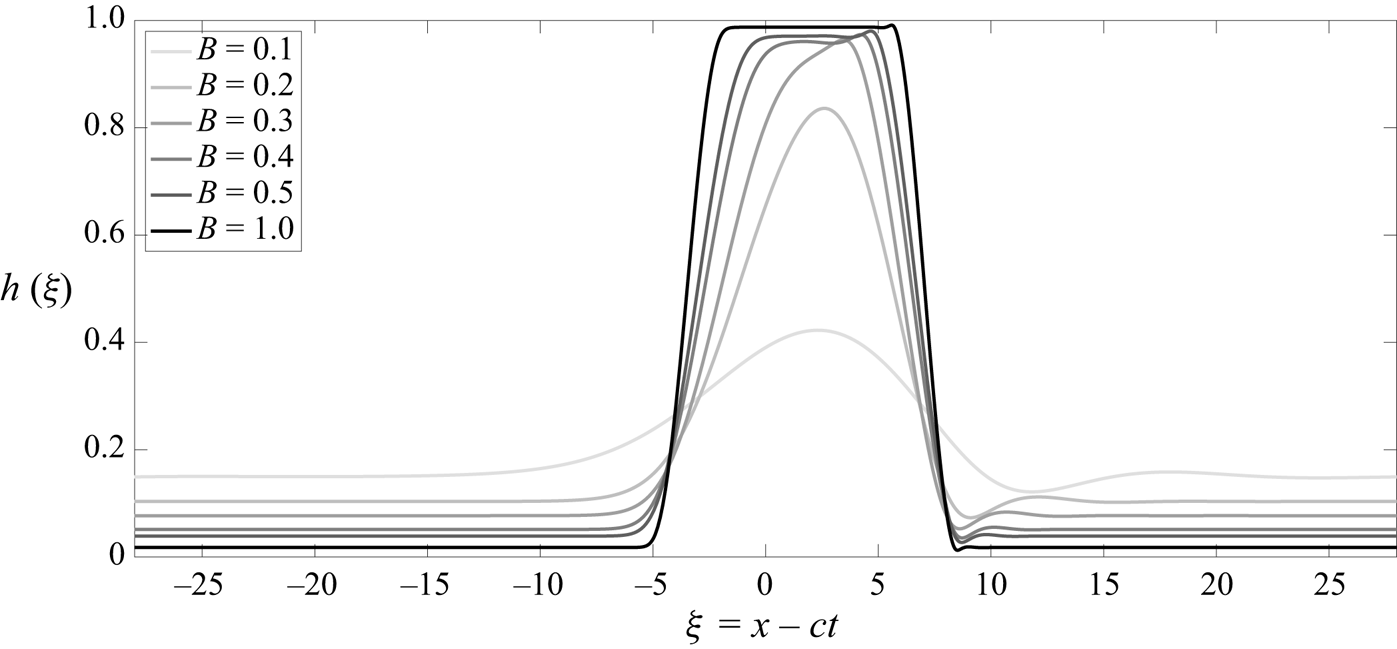
Figure 7. Interfacial travelling-wave profiles computed using AUTO for various values of  $B$. The parameters $h_0$, $m$,
$m$,  $C$ are fixed to the same values as in figure 1.
Figure 8 shows the variation of the travelling-wave speed  $c$ and the flow rate $Q$ with the Bond number $B$, for different values of the undisturbed lower fluid thickness $h_0$, capillary number $C$ and viscosity ratio $m$. Strikingly, for sufficiently large Bond number, both $c$ and $Q$ reach a plateau at the same limiting value. Furthermore, this limiting value increases with $m$ but seems to be independent of both $h_0$ and $C$. Reducing $h_0$ delays the approach to the plateau, i.e. the wave speed becomes constant at a larger value of the Bond number. These results may be used to corroborate the comments made in the previous section on finger merging. From figure 8(a) it is clear that $c$ depends strongly on $h_0$ before the plateau is attained. In a domain of fixed length $2L$, increasing $h_0$ increases the volume of the lower fluid leading to a taller finger. According to figure 8, roughly speaking $c$ increases with $h_0$ so that a taller finger travels faster. Once $h_0$ is sufficiently large for the travelling wave to (almost) touch the upper wall, the finger widens as $h_0$ increases but the wave speed remains approximately constant.
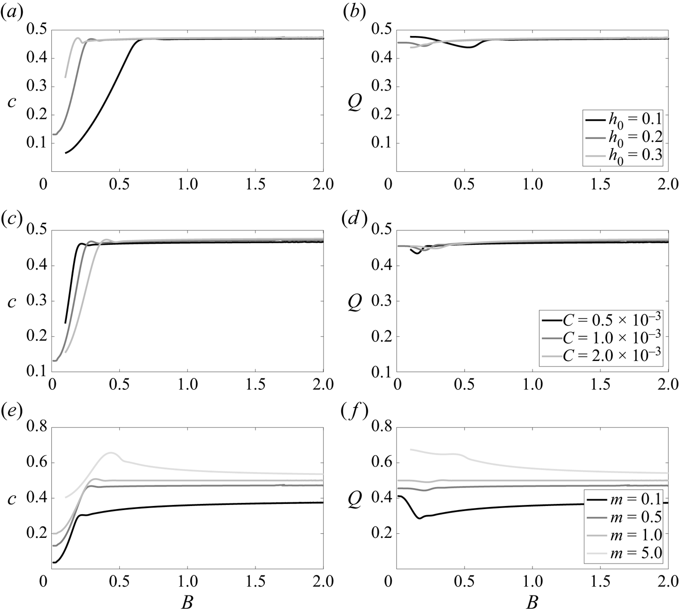
Figure 8. Variation of wave speed  $c$ and flow rate $Q$ with Bond number $B$. The various curves shown are obtained for different values of (a,b) undisturbed lower fluid thickness $h_0$, (c,d) capillary number C or (e, f) viscosity ratio m, as quoted in the respective legends (legends refer to both panels in the same row). Unless given in the legends, parameters $h_0$, $m$,
$m$,  $C$ take the same values as in figure 1.
3.4. Direct numerical simulations
Thus far our observations have been based on solutions to the model long-wave evolution equation (2.7). We have also considered values of the Bond number at which, strictly speaking, the model equation is outside of its range of validity (see the derivation in Appendix A). To provide some reassurance that our results are nonetheless relevant to a real flow, in this section we consider the full system (2.1), (2.3) and (A4) with no long-wave approximation. We solve this system numerically using the finite-element object-oriented multi-physics library oomph-lib (Heil & Hazel Reference Heil and Hazel2006a,Reference Heil and Hazelb). The flow set-up is otherwise the same and we again start our simulations from the initial condition (3.1). Some additional details about the numerical implementation in oomph-lib are provided in Appendix E.
Generally speaking the interfacial displacement evolves in time in a manner similar to that predicted by the lubrication model. For sufficiently large Bond number this includes the early finger formation, the ensuing merging dynamics and the subsequent near-wall touch-down/touch-up behaviour. The ultimate fully merged profile comprising a single wide finger is shown in figure 9. Superimposed onto this profile is that found from the travelling-wave solution to the lubrication model (cf. § 3.3) and the large-time profile obtained from the time-dependent simulation of the lubrication model (cf. § 3.1). Despite the moderate size of the Bond number (here  $B=1$ and the lubrication model strictly requires $B\ll 1$) there is excellent agreement between all three sets of results. The only minor discrepancies occur in the upper part of the finger which is slightly wider in the DNS profile (figure 9a), and in the thin film near to the lower wall (figure 9c,d) where small interfacial ripples are observed in both sets of time-dependent calculations.
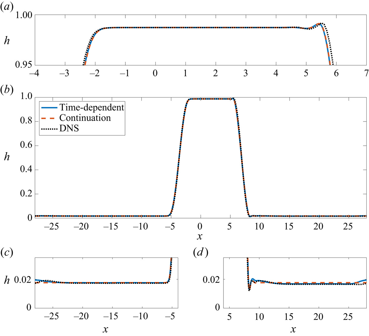
Figure 9. Comparison of interfacial profiles obtained from time-dependent calculations of the lubrication model, travelling-wave calculations of the same model and DNS of the Navier–Stokes equations. Each solution has been shifted to the right by an appropriate distance for better visualisation. The solution over the whole computational domain in shown in (b) with magnifications thereof illustrated in (a,c,d). Parameter values for  $h_0$, $m$,
$m$,  $C$,
$C$,  $B$ are the same as in figure 1.
Inspired by the good agreement seen in figure 9 between model results and DNS, we performed extensive numerical simulations for a range of Bond numbers to establish the predictive power of the model. A comparison between numerical results obtained from time-dependent simulations of the model evolution equation (2.7) and DNS can be found in figure 10. In figure 10(a), the maximum absolute error is shown as a function of the Bond number, found by calculating the difference between the two final-time interfacial profiles. An overall trend of growing error for increasing Bond number is evident, indicating that the model will eventually (for much larger  $B$) not be able to capture the ‘true’ dynamics. Figure 10(b) demonstrates that the amplitude of the two solutions is almost identical for all Bond numbers considered. For $B\gtrapprox 0.4$, the interfacial structure almost touches both channel walls and the amplitude approaches the value 1 (cf. figure 8a). This allows us to conclude that the apparent increase in error at higher Bond numbers is mainly due to width disparity between the fingers, similar to that seen in figure 9(a).

Figure 10. Comparison between numerical results obtained from time-dependent simulations of the model evolution equation (2.7) and DNS, for various Bond numbers. (a) Maximum absolute error found by calculating the difference between the two final-time interfacial profiles (model and DNS). (b) Solution amplitude found by taking the difference between the interfacial maximum and minimum at the final time. The parameters  $h_0$, $m$,
$m$,  $C$ are fixed to the same values as in figure 1.
4. Asymptotic analysis for large Bond number
Encouraged by the results in § 3, and in a bid to further understand the plateauing behaviour seen in figure 8, we now present an asymptotic analysis of the fully merged large-time travelling-wave state in the limit of large Bond number using the lubrication model.
We start by integrating equation (3.2) and using the definition of the flux in (2.7b), giving
 \begin{equation} q = \mathscr{D}^{{-}1}\left( mh^2H_1 + \tfrac{1}{3}h^3(1-h)H_2\mathcal{F} \right) = ch - \mathscr{C}, \quad \text{for some constant } \mathscr{C}, \end{equation}
where the first term on the right-hand side is the additional flux in the lower layer introduced by the shift in reference frame. Seeking a solution in the limit  $B\to \infty$ to support the results found in §§ 3.1–3.3, we divide the expected wide-finger solution into a number of asymptotic regions as shown in figure 11. This includes two transition regions ${{T_L}}$, ${{T_R}}$ in which the profile ascends/descends from one wall to the other (here, subscripts ${L}$ and ${R}$ denote ‘left’ and ‘right’); two flat thin-film regions ${{F_D}}$ and ${{F_U}}$ (here, subscripts ${D}/{U}$ mean down/up); and four connection regions ${{C_{RD}}}$, ${{C_{RU}}}$, ${{C_{LD}}}$, ${{C_{LU}}}$ that match the right/left transition regions to the down/up thin-film regions.

Figure 11. Sketch of the saturated interfacial profile of width  $\mathscr {L}$, with the various asymptotic regions. The dashed vertical lines indicate locations of matching between solutions in the different regions. Key to region names: ${T_R/T_L}$, right/left transition regions; ${F_D/F_U}$, down/up flat-film regions; ${C_{RD}/C_{RU}/C_{LD}/C_{LU}}$, right/left and down/up connection regions.
4.1. Transition regions  ${{T_R}}$ and ${{T_L}}$


We suppose there exist two transition regions in which (asymptotically) the two walls are connected to each other by a section of the interface which meets them at zero contact angle. In both of these regions the interface has a relatively steep slope. We seek a solution in the form
 \begin{equation} h = \mathscr{H}(\zeta),\quad {\rm with}\quad \xi = B^{{-}1/2}\zeta \quad \text{in }{{T_R}}; \quad \xi ={-}\mathscr{L} - B^{{-}1/2}\zeta \quad \text{in }{{T_L}}, \end{equation}
where  $\mathscr {H}$ is to be found, $\zeta =\textit {O}{\left (1 \right )}$ and $\mathscr {L}$ is the width of region ${F_U}$ (see figure 11). We note that the scaling of $B^{-1/2}\ll 1$ for the $\xi$ coordinate was chosen to retain the effect of surface tension at leading order, by ensuring the balance of the two terms on the right-hand side of (2.8d). In the coordinate rescalings (4.2b,c), the origin of $\xi$ is assumed to be in region ${T_R}$ and hence (4.2c) is essentially a shift of (4.2b) by a distance $\mathscr {L}$. The value of $\mathscr {L}$ can be estimated analytically by noticing that almost all the volume of the lower fluid is included in the finger. The volume of the finger is approximately $\mathscr {L}$ (the dimensionless height of the channel is 1), and this should be equal to the lower fluid volume in the undisturbed state. Therefore at leading order, $\mathscr {L}=2Lh_0$, where $2L$ is the domain length and $h_0$ is the undisturbed lower fluid height.
We assume that  $m$,
$m$,  $C$ and $Q$ are of order 1, and that $c=\textit {O}{\left (1 \right )}$ and $\mathscr {C}=o{\left (B^{3/2} \right )}$ (these latter scalings will be confirmed later). Then (4.1) becomes at leading order
 \begin{equation} \mathscr{H}_\zeta + \mathscr{H}_{\zeta \zeta \zeta} = 0, \end{equation}
noting that  $\mathscr {D}$ and $H_2$ are positive for $0<\mathscr {H}<1$. Assuming a solution in which the interface meets each wall with zero contact angle, then
 \begin{equation} \mathscr{H} = \frac{1}{2}(1 - \sin\zeta), \quad \text{over } -\frac{\rm \pi}{2}<\zeta<\frac{\rm \pi}{2}. \end{equation}
For later reference, it is important to note that
 $$\begin{align} \mathscr{H} &\sim \frac{1}{4}\left(\zeta - \frac{\rm \pi}{2}\right)^2, \quad \text{as } \zeta \to \frac{\rm \pi}{2}, \end{align}$$
 $$\begin{align}\mathscr{H} &\sim 1 - \frac{1}{4}\left(\zeta + \frac{\rm \pi}{2}\right)^2, \quad \text{as } \zeta \to -\frac{\rm \pi}{2}. \end{align}$$
In both transition regions the limit  $\zeta \to \pm {\rm \pi}/2$ corresponds to approaching the film near the lower/upper wall, respectively.
4.2. Flat-film regions ${F_D}$ and ${F_U}$


In the flat thin-film regions against the lower/upper walls (these regions lie outside/inside the finger), the film is of approximately uniform thickness and we take, respectively,
 \begin{equation} h = B^{{-}1}H_{D} \quad \text{or} \quad h = 1 - B^{{-}1}H_{U}, \end{equation}
where  $H_{D}$ and $H_{U}$ are both constant. The scaling of $B^{-1}$ is chosen for matching purposes as we will see later. In region ${F_D}$, (2.7b) implies $q\sim B^{-2}$, and so the right-hand side dominates in (4.1) and the flat-film thickness is found to be
 \begin{equation} H
_{D} = \frac{\hat{\mathscr{C}}}{c},
\end{equation}
\begin{equation} H
_{D} = \frac{\hat{\mathscr{C}}}{c},
\end{equation}where we have defined
 \begin{equation} \mathscr{C}=B^{{-}1}\hat{\mathscr{C}}. \end{equation}
In region  ${F_U}$, we expand $q$ in terms of $B^{-1}$, apply the scaling (4.8) in (4.1) and disregard terms of $\textit {O}{\left (B^{-2} \right )}$, resulting in
 \begin{equation} Q - B^{{-}1}H_{U} = c - B^{{-}1}\left( cH_{U} + \hat{\mathscr{C}} \right). \end{equation}
Hence the appropriate balance at  $\textit {O}{\left (1 \right )}$ and $\textit {O}{\left (B^{-1} \right )}$ gives, respectively,
 \begin{equation} Q = c \quad \text{and} \quad H_{U} = \frac{\hat{\mathscr{C}}}{1-c} = \frac{c}{(1-c)}H_{D}, \end{equation}
on using (4.7). The leading-order relationship between  $c$ and $Q$ in (4.10a) has already been noted in the results of figure 8.
4.3. Connection regions ${C_{RD}}$ and ${C_{RU}}$


Here we write
 \begin{equation} h = B^{{-}1}\tilde H(z) \quad \text{or} \quad h = 1-B^{{-}1}\hat H(z), \quad \text{and} \quad \xi ={\pm} \left( B^{{-}1/2}\frac{\rm \pi}{2} + B^{{-}1}z \right), \end{equation}
where (4.11a,b) are introduced in regions  ${C_{RD}}/{C_{RU}}$ (near the lower/upper walls), respectively, and the plus/minus signs in (4.11c) apply in the respective regions ${C_{RD}}/{C_{RU}}$.
Taking Taylor expansions with respect to  $B^{-1}$ in the various functions used to define the flux $q$ in (2.7b), and substituting in (4.1), provides the leading-order balance in each connection region. In particular, accounting for (4.8), in region ${C_{RD}}$ we find at $\textit {O}{\left (B^{-1} \right )}$
 \begin{equation} \frac{1}{3C}\tilde H^3 \tilde H_{zzz} = c \tilde H - \hat{\mathscr{C}}, \end{equation}
and in region  ${C_{RU}}$ we recover (4.10a) at $\textit {O}{\left (1 \right )}$, while at $\textit {O}{\left (B^{-1} \right )}$ we get
 \begin{equation} \frac{1}{3mC}\hat H^3\hat H_{zzz} = (1-c)\hat H - \hat{\mathscr{C}}. \end{equation}
Making use of (4.7) and (4.10b), we rescale by writing  $\{\tilde H,\hat H\} = \{H_{D},H_{U}\} H$ and $z = \beta _{\{{D},{U}\}} Z$, where $\beta _{D}=H_{D}/(3Cc)^{1/3}$ and $\beta _{U}=H_{U}/(3mC(1-c))^{1/3}$. Then (4.12) both reduce to the Landau–Levich equation (Landau & Levich Reference Landau and Levich1942, see also Bretherton Reference Bretherton1961)
 \begin{equation} H^{'''} = \frac{H-1}{H^3}, \end{equation}
where a prime denotes a derivative with respect to  $Z$.
$Z$.
The far-field conditions follow by matching to the solution in transition region  ${T_R}$ and to the flat-film solution at the walls. Reconciling the scalings (4.2b) and (4.11c), and using (4.5) and (4.6), the required matching conditions in regions ${C_{RD}}/{C_{RU}}$ are
 \begin{equation} H \sim \frac{1}{2}\mathscr{A}_{\{{D},{U}\}} Z^2 \quad \text{as } Z\to-\infty \quad \text{and} \quad H \sim 1 \quad \text{as } Z\to \infty, \end{equation}
where
 \begin{equation} \mathscr{A}_{D} = \frac{\beta_{D}^2}{2H_{D}} \quad \text{and} \quad \mathscr{A}_{U} = \frac{\beta_{U}^2}{2H_{U}}. \end{equation}
The first and second conditions in (4.14a,b) effect the matches with the transition region  ${T_R}$ and with the flat thin-film regions ${F_D}$, ${F_U}$, respectively. The connecting region problems near the right transition region thus require the solution of the Landau–Levich equation (4.13) subject to the matching conditions (4.14a,b). This problem appears in a number of related studies including the dragging of a liquid by a moving plate (Landau & Levich Reference Landau and Levich1942), the motion of long bubbles in horizontal tubes (Bretherton Reference Bretherton1961) and the capillary draining of annular films in horizontal tubes (Hammond Reference Hammond1983; Lister et al. Reference Lister, Rallison, King, Cummings and Jensen2006) and vertical tubes (Jensen Reference Jensen2000). It has a one-parameter family of solutions, meaning that $\mathscr {A}_{\{{D},{U}\}}$ cannot be determined at this stage.
4.4. Connection regions ${C_{LD}}$ and ${C_{LU}}$


Working as in the previous section, we write
 \begin{align} h = B^{{-}1}\tilde{\mathscr{H}}(z) \quad \text{or} \quad h = 1-B^{{-}1}\hat{\mathscr{H}}(z), \quad \text{and} \quad \xi ={-}\mathscr{L} \pm \left({-}B^{{-}1/2}\frac{\rm \pi}{2} + B^{{-}1}z \right), \end{align}
where  $\mathscr {L}$ was introduced in (4.2c). The scalings (4.16a,b) are applied in regions ${C_{LD}}/{C_{LU}}$ (near the lower/upper walls), respectively, and the plus/minus signs in (4.16c) apply in the respective regions ${C_{LD}}/{C_{LU}}$.
Introducing the same scalings as before,  $\{\mathscr {H},\tilde{\mathscr{H}}\} = \{H_{D},H_{U}\} H$ and $z = \beta _{\{{D},{U}\}} Z$, we again obtain the Landau–Levich equation (4.13). The matching conditions are
 \begin{equation} H \sim \frac{1}{2}\mathscr{A}_{\{{D},{U}\}} Z^2 \quad \text{as } Z\to\infty \quad \text{and} \quad H \sim 1 \quad \text{as } Z\to-\infty. \end{equation}
The asymptotic problem given by (4.13) and (4.17a,b) admits a unique solution and therefore  $\mathscr {A}_{D}=\mathscr {A}_{U}$. We find numerically that these constants are equal to $0.643$, which agrees with the value quoted elsewhere in the literature (e.g. Bretherton Reference Bretherton1961; Jensen Reference Jensen2000; Lister et al. Reference Lister, Rallison, King, Cummings and Jensen2006).
4.5. Comparison with numerical solutions
Since  $\mathscr {A}_{D}=\mathscr {A}_{U}$, it follows from (4.15a,b) that an explicit formula can be obtained for the wave speed at leading order (using also the definitions of $H_{D}$ and $H_{U}$ from (4.7) and (4.10b)), given by
 \begin{equation} c = \frac{m^{2/5}}{1+m^{2/5}}. \end{equation}
It is surprising that  $c$ depends only on the viscosity ratio, but this is in line with the results presented in § 3.3, in particular figure 8. The relationship (4.18) is plotted in figure 12. The wave speed varies rapidly with $m$ when $m<1$ and the lower fluid is the more viscous. Note that $0< c<1$ and so the wave speed is less than the wall speed (which has been used to non-dimensionalise velocities); in particular $c=1/2$ when $m=1/2$ so that the wave propagates at half the wall speed for equal-viscosity fluids. These remarks agree with the results in figure 8.

Figure 12. Variation of the interfacial wave speed  $c$ against the viscosity ratio $m$, according to the asymptotic result in (4.18).
Since  $\mathscr {A}_{D}=\mathscr {A}_{U}=0.643$, it follows that the as yet undetermined constant $\hat{\mathscr{C}}$ is given by
 \begin{equation} \hat{\mathscr{C}} = 2.675 \, C^{2/3} c^{5/3}, \end{equation}
where  $c$ is given by (4.18). This result may be combined with (4.6), (4.7) and (4.10b) to yield an estimate for the thin-film thickness in regions ${F_D}$, ${F_U}$ for a particular value of $B$.
$B$.
We conclude this section by comparing the predictions of the present asymptotic analysis with numerical solutions of the lubrication model and of the full equations via DNS. To facilitate this comparison, we fix the parameters to the same values that were used in the numerical computations in § 3, namely  $h_0=0.2$, $m=0.5$, $C=10^{-3}$, and we take a moderate value for the Bond number such as $B=1$. Setting $m=0.5$ in (4.18) yields the leading-order prediction for the wave speed $c=0.43$. The numerically computed speed for the lubrication model is approximately $c=0.4725$; this was obtained from a time-dependent simulation of the lubrication model (2.7) and it was confirmed by a travelling-wave calculation as described in § 3.3; see, in particular, figure 8. The corresponding wave speed obtained from DNS is approximately $c_{DNS}=0.4723$. Once again we note that the lubrication model agrees well with full DNS even for Bond numbers outside its strict range of validity.
Using these results and taking the same parameter values in (4.19), (4.7), (4.10b) and then (4.6), we find the individual film thicknesses to be  $h_{FD}=0.015$ and $h_{FU}=0.012$ near the down/up walls, respectively, while the numerically computed values from the lubrication model are 0.0176 and 0.0126, respectively, and the corresponding DNS values are approximately 0.0175 and 0.0127. Clearly the results obtained from simulations of the lubrication model and DNS are almost identical, and they are in good agreement with the asymptotic results.
Finally we compare the numerical solution of the asymptotic problem in each connection region with that obtained via a time-dependent simulation of the lubrication model. Numerically solving the Landau–Levich equation (4.13) with far-field conditions (4.14a,b) or (4.17a,b) gives the solutions shown with the red curves in figure 13 (the results have been scaled back to the original variables). The solution obtained from time-dependent simulations is superimposed with black curves (this is the same profile shown in figure 1f), providing good agreement between the two sets of results.

Figure 13. Solution to the asymptotic problem in the (a) left and (b) right connection regions, plotted for the same parameter values used in previous figures ( $h_0=0.2$, $m=0.5$, $C=10^{-3}$, $B=1$), and shown with red dashed curves. The black solid curves correspond to the time-dependent results. The asymptotic results have been rescaled back to the original variables, $h=h(\xi )$, by using the appropriate values for $\beta _{\{{D},{U}\}}$ and scalings in (4.11), and have been also shifted horizontally in order to match the spatial location of the connection regions as seen in figure 1( f).
5. Conclusions
We have considered the RT instability that arises at the interface between two immiscible viscous fluids in a channel that is undergoing a shearing motion due to the translation of the upper wall. We have derived a nonlinear lubrication equation that is appropriate for describing the evolution of the fluid–fluid interface on the assumption that the wavelength of the interfacial disturbances is large in comparison with the channel height. For any positive Bond number, meaning that the fluids are unstably stratified and RT instability is present, a small-amplitude perturbation to the initially flat interface grows to develop a highly nonlinear structure. Numerical computations performed assuming periodic boundary conditions, and on the assumption that there is no pressure drop across one period, demonstrated the appearance of a pronounced finger-like pattern with the number of fingers in one period accurately predicted by linear stability theory. The fingers in general have different heights and travel at different speeds (taller fingers travel faster) so that inter-finger collisions and merging events occur. As merging continues the number of fingers gradually reduces leaving finally a residual finger which roughly encompasses all of the lower fluid volume. This behaviour is similar to the coarsening dynamics of roll wave structures propagating down an inclined plane (Chang et al. Reference Chang, Demekhin and Kalaidin2000; Razis et al. Reference Razis, Edwards, Gray and van der Weele2014). At sufficiently large Bond number the final finger spans the entire channel cross-section so that it essentially segregates the two fluids; the width of the finger is set by the initial volume ratio of the two fluids in the periodic domain. The finger propagates as a more-or-less fixed-form travelling wave, although thin-film coatings of each fluid adjacent to the channel walls are unsteady. Their highly irregular behaviour is reminiscent of the chaotic dynamics that characterises the evolution of thin films in certain parameter regimes (Kawahara Reference Kawahara1983; Kawahara & Toh Reference Kawahara and Toh1988; Kalogirou & Papageorgiou Reference Kalogirou and Papageorgiou2016). We have demonstrated analytically that touch-down/touch-up of the interface with the channel walls does not occur in finite time, and our numerics in fact indicate that the minimum gap almost saturates in time due to the presence of a base shear flow.
The existence of fully steady travelling-wave solutions was confirmed by a continuation procedure carried out using AUTO-07p (Doedel & Oldman Reference Doedel and Oldman2009) in a moving reference frame. These calculations successfully reproduced the large-time interfacial profile attained in the unsteady simulations (overlooking the persistent chaotic behaviour in the thin-film regions). Furthermore they demonstrated that the wave speed and the total channel flux both reach a plateau as the Bond number is increased to a relatively large value (in fact roughly around  $B=1$), and that this plateau depends only on the size of the viscosity ratio. This behaviour was further investigated via a large-Bond-number asymptotic analysis that revealed the finer details of the post-coarsening final-state travelling wave and confirmed that the wave speed and channel flux approach the same value in the large- $B$ limit. The asymptotic structure includes localised depression and capillary ridge features that occur in narrow connection regions close to the wall wherein the system is well approximated by the Landau–Levich equation (Landau & Levich Reference Landau and Levich1942). In this regard our analysis resembles that presented by other authors for similar problems (e.g. Bretherton Reference Bretherton1961; Hammond Reference Hammond1983; Jensen Reference Jensen2000; Lister et al. Reference Lister, Rallison, King, Cummings and Jensen2006).
Although we have focused our attention on relatively large values of the Bond number, our lubrication equation is formally only valid for small values of this parameter (in that case, smaller-amplitude travelling waves that do not straddle the whole channel height are achieved; see the light grey curve in figure 7 for an example using  $B=0.1$). With this in mind we have also carried out time-dependent simulations of the full Stokes equations. These were found to be in excellent agreement with the predictions of the lubrication model, even for moderate sized Bond number. Both qualitative and quantitative agreement was found, for example in the estimation of the final-state travelling-wave speed and the residual film thickness at the channel walls. For sufficiently large Bond number, the model predictions are not expected to accurately characterise the dynamics (cf. figure 10). In fact, for large enough Bond number we expect to see features such as interfacial break-up and droplet formation (Kalogirou, Cimpeanu & Blyth Reference Kalogirou, Cimpeanu and Blyth2020).
The stability of the final travelling-wave states has not been addressed here directly. However, since for both the lubrication model and the full Stokes equations the waves emerge as the large-time limit of an initial value problem, this suggests that they are stable to two-dimensional disturbances; although loss of stability to perturbations of wavelength greater than the length of our computational domain cannot be ruled out. The stability of the system to transverse perturbations, however, remains to be investigated (e.g. Mavromoustaki, Matar & Craster Reference Mavromoustaki, Matar and Craster2011). While in this paper we have focused on single-finger saturated states, multi-finger states can also be attained in unsteady simulations through particular choices of the initial condition, and these are the subject of our ongoing research. A further point of interest suggested by the asymptotic analysis of § 4 concerns the possibility of finding shock-like solutions wherein the interfacial level changes smoothly from one constant value to another from upstream to downstream in the manner of a hydraulic fall. It should be noted that the analysis of § 4 does not determine the width of the travelling wave,  $\mathscr {L}$, this being set effectively by the volume ratio of the two fluids in the periodic domain. With this in mind, by extending the domain length to infinity, shock solutions of the kind computed for an inclined channel with stationary walls by Mavromoustaki et al. (Reference Mavromoustaki, Matar and Craster2010), using the entropy-flux approach of Bertozzi, Münch & Shearer (Reference Bertozzi, Münch and Shearer1999), could presumably be constructed. This is left as a topic for future investigation.
Supplementary movie
Supplementary movie is available at https://doi.org/10.1017/jfm.2022.1070.
Acknowledgements
We thank Professor A. Hazel for the help with setting up the oomph-lib code which was used for the DNS.
Funding
This research received no specific grant from any funding agency, commercial or not-for-profit sectors.
Declaration of interests
The authors report no conflict of interest.
Appendix A. Derivation of the lubrication equation
A lubrication equation for the evolution of a disturbance at the interface can be derived by assuming that the wavelength of the disturbance is much larger than the channel height. This suggests a rescaling of the horizontal coordinate and the introduction of a slow time scale as follows:
 \begin{equation} \chi = \epsilon\,x, \quad \tau = \epsilon\,t, \quad \text{with} \ \epsilon\ll1, \end{equation}
where  $\epsilon$ is the height-to-wavelength ratio and $\chi$, $\tau$ are of $\textit {O}{\left (1 \right )}$. The flow velocities and pressures are expanded in the following manner (Tilley et al. Reference Tilley, Davis and Bankoff1994):
 \begin{equation} u_j = u_j^{(0)} + \epsilon\,u_j^{(1)}, \quad v_j = \epsilon\,v_j^{(0)} + \epsilon^2v_j^{(1)}, \quad p_j = \epsilon^{{-}1}p_j^{(0)} + p_j^{(1)}. \end{equation}
The following rescaling for the Bond and capillary numbers is also introduced, in order to keep the effects of gravity and surface tension in the leading-order dynamics (e.g. Mavromoustaki et al. Reference Mavromoustaki, Matar and Craster2010):
 \begin{equation} B = \epsilon^2\tilde{B}, \quad C = \epsilon^3\tilde{C} \quad \text{with} \ \tilde{B}, \tilde{C} = \textit{O}{\left(1 \right)}. \end{equation}
Expansions (A2a–c) and rescalings (A1) and (A3) are substituted into the kinematic equation
 \begin{equation} h_t + \left( \int_0^{h(x,t)} u_1\,{\mathrm d} y \right)_x = 0 \quad \text{at} \ y=h(x,t), \end{equation}
the momentum and continuity equations (2.1), and the normal and tangential stress balances given in (2.3), yielding the leading-order system
 \begin{align} m_j u_{jyy}^{(0)} - p_{j\chi}^{(0)} &= 0, \quad \text{for} \ j=1,2, \end{align}
 \begin{align}p_{jy}^{(0)} + \frac{r_j}{(r-1)}\frac{\tilde{B}}{\tilde{C}}&= 0, \quad \text{for} \ j=1,2, \end{align}
 \begin{align}u_{j\chi}^{(0)} + v_{jy}^{(0)} &= 0, \quad \text{for} \ j=1,2, \end{align}
 \begin{align}u_1^{(0)} = 0, \quad v_1^{(0)} &= 0, \quad \text{at} \ y=0, \end{align}
 \begin{align}u_2^{(0)} = 1, \quad v_2^{(0)} &= 0, \quad \text{at} \ y=1, \end{align}
 \begin{align}u_1^{(0)} &= u_2^{(0)}, \quad \text{at} \ y=h(\chi,\tau), \end{align}
 \begin{align}mu_{2y}^{(0)} - u_{1y}^{(0)} &= 0, \quad \text{at} \ y=h(\chi,\tau), \end{align}
 \begin{align}p_2^{(0)} - p_1^{(0)} &= \frac{1}{\tilde{C}}h_{\chi\chi}, \quad \text{at} \ y=h(\chi,\tau), \end{align}
 \begin{align}\int_0^h u_1^{(0)}\,{\mathrm d} y + \int_h^1 u_2^{(0)}\,{\mathrm d} y &= Q(t). \end{align}
Integrating (A5b) in  $y$ gives
 \begin{equation} p_j^{(0)} ={-} \frac{r_j}{(r-1)}\frac{\tilde{B}}{\tilde{C}}y + P_j, \end{equation}
where the functions  $P_j(\chi,\tau )$ are related to each other, via condition (A5h), as
 \begin{equation} P_2 = P_1 + F,\quad{\rm where}\ F = \tilde{C}^{{-}1}(\tilde{B} h + h_{\chi\chi}). \end{equation}
The momentum equations (A5a) can then be integrated in  $y$ twice to obtain
 \begin{equation} u_1^{(0)} = \frac{1}{2}y^2P_{1\chi} + yA_1, \quad u_2^{(0)} = \frac{1}{2~m}(y^2-1)P_{2\chi} + (y-1)A_2 + 1, \end{equation}
where the no-slip boundary conditions at the walls (A5d), (A5e) have been applied. The arbitrary functions  $A_j=A_j(\chi,\tau )$ are determined by using the two conditions (A5f), (A5g), and then using (A7a). Their expressions simplify to
 \begin{equation} A_2 = \frac{1}{m}\left( A_1 - h F_\chi \right), \quad A_1 = \frac{ 2m - (1+(m-1)h^2)P_{1\chi} - (h-1)^2 F_\chi}{2(1+(m-1)h)}. \end{equation}
 The continuity equations (A5c) can be used to provide similar expressions for the leading-order vertical velocity perturbations; integrating in  $y$ and using the no-penetration boundary conditions at the walls (A5d), (A5e), yields
 \begin{equation} v_1^{(0)} ={-}\frac{1}{6}y^3P_{1\chi\chi} - \frac{1}{2}y^2A_{1\chi}, \quad v_2^{(0)} ={-}\frac{1}{6m}(y^3-3y+2)P_{2\chi\chi} - \frac{1}{2}(y^2-2y+1)A_{2\chi}. \end{equation}
It remains to use the integral constraint (A5i) to determine the leading-order pressure gradient, finding
 \begin{align} P_{1\chi} &= \mathscr{D}^{{-}1} \left[ - 6m\left( (m-1)h^2 - 2(m-1)h - 1 \right) \right. \nonumber\\ &\left.\quad + (h-1)^2\left( (m-1)h^2+2(1-2m)h-1 \right)F_\chi - 12m\left( (m-1)h+1 \right)Q(t) \right], \end{align}
where  $\mathscr {D}$ is defined in (2.8a). We note that the flow rate $Q(t)$ can be found by satisfying a periodicity condition on the pressure (Ooms et al. Reference Ooms, Segal and Cheung1985; Blyth & Pozrikidis Reference Blyth and Pozrikidis2004; Kalogirou & Blyth Reference Kalogirou and Blyth2020), e.g.
 \begin{equation} \int_{{-}L}^{L} P_{1\chi}\,{\mathrm d}\kern0.7pt x = P_1(L,\tau) - P_1({-}L,\tau) = 0, \end{equation}
or equivalently fixing the pressure drop in the streamwise direction to be zero over a specified domain of length  $2L$.
$2L$.
With the solution for  $P_{1\chi }$ known from (A11), function $A_1$ and then $A_2$ can be found from (A9a,b) and finally $P_{2\chi }$ can be found using (A7a). The leading-order horizontal velocities in each fluid can then be obtained from (A8). The evolution of the interfacial displacement is found by inserting the leading-order horizontal velocity (A8a) into the kinematic equation (A4), and is given by
 \begin{equation} h_\tau + q_\chi = 0 \quad \text{with} \ q = \frac{1}{6}P_{1\chi}h^3 + \frac{1}{2}A_1h^2. \end{equation}
The evolution equation (A13) can be scaled back to the original variables  $x$,
$x$,  $t$ and the result is given in (2.7), which also includes the original parameters $B$,
$B$,  $C$. We note that the expression for $q$ in (2.7) is the same as that in (A13), but it is written in a different form for convenience.
Appendix B. Linear stability theory
The growth rate of (2.7) is found by writing  $h=h_0+A\exp ({\rm i}Kx+\sigma t)+ \text {c.c.}$ (complex conjugate) for some small amplitude $A$. Here, $\sigma$ is the growth rate which is generally a complex number and $K$ is the wavenumber, assumed real. Substituting this expression into (2.7) yields
 \begin{equation} \sigma + {\rm i}K\mathscr{D}(h_0)^{{-}1}\left( mh_0^2H_1(h_0) + \frac{1}{3C}h_0^3(1-h_0)^3H_2(h_0)({\rm i}KB-{\rm i}K^3) \right) = 0. \end{equation}
The growth rate is then provided by the real part of  $\sigma$ and is given by
 \begin{equation} \mathrm{Re}(\sigma) = K^2(B-K^2)\frac{ h_0^3(1-h_0)^3H_2(h_0) }{ 3C \mathscr{D}(h_0) }. \end{equation}
Since  $0< h_0<1$, and $\mathscr {D}>0$, $H_2>0$, the growth rate is clearly positive if $K< K_c$, where the cut-off wavenumber is $K_c=\sqrt {B}$. The growth rate attains its maximum at the point where $\partial _K(\mathrm {Re}(\sigma ))=0$, which is located at $K_{max}=\sqrt {B/2}$.
Appendix C. Weakly nonlinear analysis
Writing  $h(x,t)=\delta \big(H_0+\delta H(x,t)\big)$ in (2.7), with $\delta \ll 1$, $H_0=\textit {O}{\left (1 \right )}$ is constant and $H=\textit {O}{\left (1 \right )}$, we find
 \begin{align}
\delta^2H_t &+ \left[ \alpha_1H\delta^3 + \left(\alpha_2H+\alpha_3H^2\right)\delta^4\right.\nonumber\\ &\quad\left. + \left(\alpha_4H+\alpha_5H^2+\alpha_{6}H_x+\alpha_{7}H_{xxx}\right)\delta^5
+ \textit{O}{\left(\delta^6 \right)} \right]_x = 0,
\end{align}
\begin{align}
\delta^2H_t &+ \left[ \alpha_1H\delta^3 + \left(\alpha_2H+\alpha_3H^2\right)\delta^4\right.\nonumber\\ &\quad\left. + \left(\alpha_4H+\alpha_5H^2+\alpha_{6}H_x+\alpha_{7}H_{xxx}\right)\delta^5
+ \textit{O}{\left(\delta^6 \right)} \right]_x = 0,
\end{align}
where  $\alpha _i=\alpha _i(H_0,m,Q(t))$ for $i=1,\ldots,5$, and $\alpha _{6}=H_0^3B/(3C)$, $\alpha _{7}=H_0^3/(3C)$. The numerical evidence suggests that the flow rate $Q$ is a constant in the large-time limit when the travelling-wave structure is reached (see figure 8), so we treat $Q(t)$ as a constant to leading order. The second term on the left-hand side can be then removed by taking a Galilean transformation of the form $\hat {x}=x-\delta \alpha _1t$. A slow-time scale is introduced by $\hat {t}=\delta ^2t$, and the capillary number is rescaled as $C=\delta C_0$ (Kalogirou & Papageorgiou Reference Kalogirou and Papageorgiou2016), and so the evolution equation (C1) becomes at leading order
 \begin{equation} H_{\hat{t}} + \alpha H_{\hat{x}} + 2\alpha_3HH_{\hat{x}} + \frac{H_0^3}{3C_0}\left(BH_{\hat{x}\hat{x}}+H_{\hat{x}\hat{x}\hat{x}\hat{x}}\right) = 0, \end{equation}
where  $\alpha$ is a time-dependent coefficient which depends on the first-order correction to $Q(t)$.
Appendix D. Boundedness of solutions
The results in § 3.1 suggest that when the interface gets close to one of the channel walls, then the  $\mathcal {F}$ term in (2.8d) dominates the evolution equation (2.7); cf. figure 4. To examine near-wall touch-down/touch-up, it is therefore sufficient to keep only the dominant terms in the evolution equation, which reduces to
 \begin{equation} h_t + \left( \frac{1}{3}h^3(1-h)^3\mathscr{D}^{{-}1}H_2\mathcal{F} \right)_x = 0, \end{equation}
where we recall that  $\mathcal {F}=C^{-1}(Bh_x + h_{xxx})$. A similar equation has been obtained in related studies investigating the RT instability in thin viscous films (Yiantsios & Higgins Reference Yiantsios and Higgins1989), also in the presence of electric fields (Tseluiko & Papageorgiou Reference Tseluiko and Papageorgiou2007; Anderson et al. Reference Anderson, Cimpeanu, Papageorgiou and Petropoulos2017). In particular, if the interface is in the vicinity of the lower or upper wall, that is, $h\approx 0$ or $h\approx 1$, the evolution equation (D1) is similar to those previously derived by Tseluiko & Papageorgiou (Reference Tseluiko and Papageorgiou2007) or Anderson et al. (Reference Anderson, Cimpeanu, Papageorgiou and Petropoulos2017), respectively, if the influence of electric fields is omitted in both of these studies.
Here we aim to prove that smooth solutions are uniformly bounded. We follow closely the proof of Tseluiko & Papageorgiou (Reference Tseluiko and Papageorgiou2007) for an electrified film. We begin by defining the functional
 \begin{equation} E(h) = \frac{1}{2}C^{{-}1}\int_{{-}L}^L \left({-}Bh^2 + h_x^2 \right) \,{\mathrm d}\kern0.7pt x. \end{equation}
This can be shown to be non-increasing in time, as follows:
 \begin{align} \frac{{\mathrm d} E}{{\mathrm d} t} &= \int_{{-}L}^L C^{{-}1}\left({-}B hh_t + h_x h_{xt} \right) \,{\mathrm d}\kern0.7pt x = \int_{{-}L}^L C^{{-}1}\left( B h + h_{xx} \right)({-}h_t) \,{\mathrm d}\kern0.7pt x \nonumber\\ &= \int_{{-}L}^L C^{{-}1}\left( B h + h_{xx} \right)\left( \frac{1}{3}h^3(1-h)^3\mathscr{D}^{{-}1}H_2\mathcal{F} \right)_x \,{\mathrm d}\kern0.7pt x \nonumber\\ &={-} \int_{{-}L}^L \frac{1}{3}h^3(1-h)^3\mathscr{D}^{{-}1}H_2\mathcal{F}^2 \,{\mathrm d}\kern0.7pt x \le0, \end{align}
where we have used (D1) to replace  $h_t$, and the periodicity of $h$ to remove the boundary terms when integrating by parts. The inequality in (D3) is proved on recalling that $\mathscr {D}>0$ and $H_2>0$ from (2.8a) and (2.8c), respectively. The functional in (D2) can be written as
 \begin{equation} E(h) ={-}\frac{1}{2}C^{{-}1}B\|h\|_2^2 + \frac{1}{2}C^{{-}1}\|h_x\|_2^2 = \alpha_1 \|h\|_{H^1}^2 - \alpha_2 \|h\|_2^2, \end{equation}
where  $\alpha _1=\tfrac {1}{2}C^{-1}>0$ and $\alpha _2=\tfrac {1}{2}C^{-1}(B+1)>0$. Here, $\|h\|_2$ denotes the L $_2$-norm and $\|h\|_{H^1}^2 = \|h\|_2^2 + \|h_x\|_2^2$ is the norm defined in the $H^1$ Sobolev space comprising periodic functions in $[-L,L]$.
Using the interpolation inequality gives (e.g. Bertozzi & Pugh Reference Bertozzi and Pugh1998)
 \begin{align} \|h\|_2 \le \gamma_1 \|h\|_{H^1}^{1/3} \|h\|_1^{2/3}, \end{align}
where  $\|h\|_1$ is the L $_1$-norm and $\gamma _1$ is a positive constant. Applying Young's inequality to the right-hand side of (D5a) yields
 \begin{equation} \|h\|_2 \le \gamma_1 \left( \frac{\varepsilon}{3}\|h\|_{H^1} + \frac{2}{3\sqrt{\varepsilon}}\|h\|_1 \right), \end{equation}
where  $\varepsilon$ is a positive constant, and hence
 \begin{equation} \|h\|_2^2 \le \gamma_1^2 \left( \frac{\varepsilon^2}{9}\|h\|_{H^1}^2 + \frac{4}{9\varepsilon}\|h\|_1^2 + \frac{4\sqrt{\varepsilon}}{9}\|h\|_{H^1}\|h\|_1 \right) \le 2\gamma_1^2 \left( \frac{\varepsilon^2}{9}\|h\|_{H^1}^2 + \frac{4}{9\varepsilon}\|h\|_1^2 \right). \end{equation}
By inserting the result in (D5c) into (D4), we establish that
 \begin{equation} E(h) \ge \tilde{\alpha}_1\|h\|_{H^1}^2 - \tilde{\alpha}_2\|h\|_1^2, \quad \text{or equivalently} \quad \|h\|_{H^1}^2 \le \beta_1 E(h) + \beta_2 \|h\|_1^2. \end{equation}
Here,  $\tilde {\alpha }_1=\alpha _1-2\alpha _2\gamma _1^2\varepsilon ^2/9$, $\tilde {\alpha }_2=8\alpha _2\gamma _1^2/(9\varepsilon )$ and $\beta _1=1/\tilde {\alpha }_1$, $\beta _2=\tilde {\alpha }_2/\tilde {\alpha }_1$. We note that $\tilde {\alpha }_1$ is positive for small enough $\varepsilon$ and $\tilde {\alpha }_2>0$ for any $\varepsilon >0$, and hence we can ensure that both $\beta _1$, $\beta _2$ are positive by choosing $\varepsilon$ to be sufficiently small.
Assuming a smooth initial condition  $h(x,0)=h^{(0)}(x) \in H^1$ satisfying periodicity in the domain $[-L,L]$, then the norm $\|h\|_{H^1}$ is uniformly bounded since from (D6) we find
 \begin{equation} \|h\|_{H^1}^2 \le \beta_1 E(h^{(0)}) + \beta_2 \|h^{(0)}\|_1^2 \equiv \bar{C}, \end{equation}
using the result in (D3) and conservation of volume, i.e.  $\|h\|_1=\|h^{(0)}\|_1$, which follows immediately from (D1). This proves that the Sobolev norm of the solution $h$ is bounded for all $t>0$.
We use this boundedness result to show that the interface cannot touch the channel walls in finite time. We start by tracking the time evolution of the two spatial integrals
 \begin{equation} \frac{{\mathrm d}}{{\mathrm d} t}\int_{{-}L}^L \frac{1}{h}\,{\mathrm d}\kern0.7pt x = \int_{{-}L}^L -\frac{h_t}{h^2}\,{\mathrm d}\kern0.7pt x = \frac{2}{3}\int_{{-}L}^L h_x(1-h)^3\mathscr{D}^{{-}1}H_2\mathcal{F}\,{\mathrm d}\kern0.7pt x \end{equation}
and
 \begin{equation} \frac{{\mathrm d}}{{\mathrm d} t}\int_{{-}L}^L \frac{1}{(1-h)}\,{\mathrm d}\kern0.7pt x = \int_{{-}L}^L \frac{h_t}{(1-h)^2}\,{\mathrm d}\kern0.7pt x = \frac{2}{3}\int_{{-}L}^L h_xh^3\mathscr{D}^{{-}1}H_2\mathcal{F}\,{\mathrm d}\kern0.7pt x, \end{equation}
where in both integrals we have substituted the expression for  $h_t$ from (D1) and integrated by parts. The upper bound $\mathscr {D}^{-1}H_2\leqslant \max \{1,m^{-1}\}\equiv \mathcal {M}$ is valid for $0< h<1$ (in fact, the bound of 1 or $m^{-1}$ is approached when $h\approx 0$ or $h\approx 1$, respectively). Using this result and the definition of $\mathcal {F}$ from (2.8d), we can show that the integrals on the far right-hand sides in (D8) are bounded by
 \begin{align} \frac{2}{3}\mathcal{M} C^{{-}1} \int_{{-}L}^L h_x(Bh_x + h_{xxx})\,{\mathrm d}\kern0.7pt x &= \frac{2}{3}\mathcal{M} C^{{-}1}\left( B \|h_x\|_2^2 - \|h_{xx}\|_2^2 \right) \nonumber\\ &\leqslant a\|h_x\|_2^2 \leqslant a\|h_x\|_2^2 + a\|h\|_2^2 = a\|h\|_{H^1}^2 \leqslant a\bar{C}, \end{align}
with  $a=\tfrac {2}{3}\mathcal {M} C^{-1}B>0$. The last step in (D9) applies the uniform bound result shown earlier in (D7). We have therefore proved that the spatial integrals of $h^{-1}$ and $(1-h)^{-1}$ remain bounded over a finite time interval. This result can be used to show that a solution satisfying $0< h<1$ initially, will satisfy this condition at all (finite) times; equivalently, that is to say the interface will not touch down/up in finite time. The rest of the proof is based on Agmon's inequality (Agmon Reference Agmon1965) and can be completed in the same way as in Tseluiko & Papageorgiou (Reference Tseluiko and Papageorgiou2007).
Appendix E. Details of the oomph-lib implementation
The governing equations are discretised in space using the finite-element method and in time using the second-order-accurate backward differentiation formulae (BDF). A Newton solver is then applied to solve the fully space–time discretised system, and adaptive time stepping is employed so that a temporal root-mean-square error norm (based on the difference between a prediction and the computed solution) remains below a tolerance of  $10^{-5}$. We refer the reader to the oomph-lib webpage (Heil & Hazel Reference Heil and Hazel2006b) for more details on the methods used.
The mesh is based on quadrilateral Crouzeix–Raviart elements and the method of spines is used to approximate the nodal position of the interface at a given location. A simulation for  $B=1$ uses 600 elements in the horizontal direction and 16 elements in the vertical direction in each fluid layer. These parameters were found to be sufficient to produce accurate results, in the sense that simulations with double resolution gave interfacial profiles that are visually indistinguishable from those seen in figure 9. An example of the mesh for the highly deformed saturated state obtained for $B=1$ is depicted in figure 14. We note that smaller values of $B$ produce less deformed interfacial structures and hence require fewer elements to produce accurate results.

Figure 14. Lower fluid mesh from a DNS in oomph-lib, using 600 elements in the horizontal direction and 16 elements in the vertical direction in each fluid layer. The saturated interfacial profile shown is obtained for  $B=1$. The colour corresponds to the horizontal velocity in the lower fluid, varying from 0 (blue) on the lower channel wall to 1 (red) on the upper wall. The fluid is seen to move slightly faster than the upper wall (darker red colour) right before the capillary ridge at $x=12.5$.


 Open access