


1. Introduction
The Cauchy–Poisson problem is classical in fluid mechanics and applied mathematics. This pioneering initial-value problem for water waves is described in the textbook by Lamb (Reference Lamb1932, pp. 384–398). It is hereafter referred to as the CP problem. There are two separate subproblems of the fully linearized CP problem: (i) The primary CP problem, where the fluid starts its motion from rest, with a prescribed surface elevation. (ii) The secondary CP problem, where the fluid is forced into motion with zero initial surface elevation (initially horizontal surface). The present paper is devoted to this secondary CP problem, which we will formulate in its fully nonlinear version. The way to initiate the flow in our secondary CP problem, is to apply an instantaneous pressure impulse to the initially horizontal surface and thereafter let the nonlinear free-surface flow evolve in a uniform gravitational field.
Not much research exists on the fully nonlinear CP problem. Shinbrot (Reference Shinbrot1976) and Reeder & Shinbrot (Reference Reeder and Shinbrot1976, Reference Reeder and Shinbrot1979) performed mathematical investigations for this class of problems. Debnath (Reference Debnath1989) studied weak free-surface nonlinearities by the Lagrangian description of motion.
These mathematical papers did not consider the causal initiation of free-surface nonlinearity, which is our present focus. At infinite depth, the early time span of a gravitational time unit will be decisive for the further nonlinear process. This is known from two theoretical studies on the present class of Cauchy–Poisson problem, where a surface pressure is turned on to work on the initially horizontal surface of a semi-infinite fluid. Saffman & Yuen (Reference Saffman and Yuen1979) applied a surface pressure which was sinusoidal in space and time, but of finite duration. Their aim was to investigate numerically the highest non-breaking standing waves which are periodic in space and as close as possible to periodic in time. They found interesting results with full nonlinearity, but their dilemma was that their induced flow departed too much from strict periodicity in time. Longuet-Higgins & Dommermuth (Reference Longuet-Higgins and Dommermuth2001) realized that a similar model could be interesting for investigating the highest transient waves, which they did. They applied an instantaneous pressure impulse instead of the surface pressure of long duration studied by Saffman & Yuen (Reference Saffman and Yuen1979). Longuet-Higgins & Dommermuth (Reference Longuet-Higgins and Dommermuth2001) achieved much higher amplitudes of transient waves than are known experimentally for periodic waves (Taylor Reference Taylor1953), but they did not compute the motion after the stagnant peaks had been reached, since these peaks will experience essentially free fall which inevitably leads to surface breaking.
Our theoretical model follows the earlier work by Longuet-Higgins & Dommermuth (Reference Longuet-Higgins and Dommermuth2001), with one essential difference. They considered a spatially periodic pressure impulse (sinusoidal), while we will consider a localized pressure impulse (of the multipole type). Spatial periodicity forbids deep-water dispersion from reducing nonlinearity by shifting the energy to longer wavelengths, since the longest wavelength is that of the pressure impulse itself. Only shorter wavelengths can be triggered in these periodic models, which makes the growing of nonlinearity in time inevitable.
During the first gravitational time unit, it is not very essential whether a nonlinear flow is spatially periodic or not. The build-up of free-surface nonlinearity that our model will give during the gravitational time unit will be analogous to the previous work, but after that, it will become very different. After a gravitational time unit, we will have a dominating deep-water dispersion spreading out the non-periodic wave pattern to reduce its amplitude and make it gradually adapt to linear theory. After a couple of gravitational time units, our type of flow will become linearized, although there will be surviving signatures from the early stage where nonlinearity was crucial. These signatures will be increasingly difficult to extract as the linearized dispersive flow dominates.
The strong-impact limit of impulsive flow, which is studied here for the secondary CP problem, is essentially a slamming type of flow (Wagner Reference Wagner1932; Korobkin & Pukhnachov Reference Korobkin and Pukhnachov1988). The conventional way of modelling incompressible slamming problems (water impact) is to give the forced impulsive motion of a body entering a liquid with an initially free horizontal surface, and compute the resulting flow and the impact pressure forces that it generates on the body. The normal velocity is then the cause, and the impulsive pressure field is its effect. In the present paper we will take an opposite causal view on slamming, where an impulsive surface pressure distribution is taken as the cause, and the resulting free-surface flow is the induced effect. The present type of theory may be considered as a parallel development which is complementary to the voluminous slamming theory. A mathematical advantage with our approach is our consistent analysis of the early free-surface nonlinearities that evolve within an impulsive time scale, before gravity takes over and dominates the process.
The present work consists of two parts. In this first part we will develop an analytical small-time expansion to third order in time, in the standard Eulerian description of motion. Exact closed-form solutions will be given for two families of pressure impulses; the dipole type and the quadrupole type. Numerical simulations for the fully nonlinear free-surface flow will be presented, but only for the quadrupole type of pressure impulses because of the slow far-field decay of the dipole distributions. Comparisons between analytical and numerical results will be postponed to Part 2 of this work (Tyvand, Mulstad & Bestehorn Reference Tyvand, Mulstad and Bestehorn2021), where a second-order small-time expansion is developed in the Lagrangian description of motion. We will then show and compare two analytical and one numerical approach to the same strongly nonlinear problem, and investigate in detail how the analytical solutions fail when the free-surface nonlinearity becomes too strong.
2. Modelling assumptions and formulation
We consider an inviscid and incompressible fluid (liquid) which is initially at rest with the horizontal free surface  $z=0$. The fluid has constant depth $h$ and a free surface subject to constant atmospheric pressure. Time is denoted by $t$. Cartesian coordinates $x, y, z$ are introduced, where the $z$ axis is directed upwards in the gravity field and the horizontal $x, y$ plane defines the undisturbed free surface. The fluid layer is of infinite horizontal extent. The gravitational acceleration is $g$, and $\rho$ denotes the constant fluid density. The components of the velocity vector $\boldsymbol {v}$ are denoted by $(u,v,w)$. The surface elevation is $\eta (x,y,t)$. It is very important to note that $\eta$ by definition represents the strictly vertical motion of the mathematical free surface, not the motion of a fluid particle at the surface. This means that the following integral is zero
 \begin{equation} \int_{-\infty}^{\infty} \int_{-\infty}^{\infty} \eta(x, y) \, \textrm{d} x\, \textrm{d} y = 0, \end{equation}
since the average surface level must be constant in the absence of mass sources in the fluid domain.
We assume a forced initial flow  $w(x,y,0,0)$ at the free surface, and its forcing will be discussed in detail below. The forcing transfers a net downward momentum in the fluid, and a net energy (being equal to the kinetic energy at $t=0^{+}$), but zero mass flux, as already stated in (2.1). We will see that the forcing induces not only a vertical velocity but also horizontal velocity components at the parts of the surface where the forcing takes place. No vorticity is generated within the inviscid fluid, which implies that the flow is irrotational according to Lord Kelvin's theorem
 \begin{equation} \boldsymbol{\nabla} \times \boldsymbol{v} = 0, \end{equation}
implying the existence of a velocity potential  $\varPhi (x,y,z,t)$ so that $\boldsymbol {v} = \boldsymbol {\nabla } \varPhi$. The incompressible flow of the homogeneous fluid implies the validity of Laplace's equation
 \begin{equation} \nabla^{2} \varPhi = 0, \end{equation}
in the entire fluid domain. From the equation of motion Bernoulli's equation follows
 \begin{equation} \frac{p-p_{atm}}{\rho} + \frac{\partial \varPhi}{\partial t} + \frac{1}{2} \vert \boldsymbol{\nabla} \varPhi \vert^{2} + g z = 0. \end{equation}
The atmospheric pressure  $p_{atm}$ appears as an integration constant. The flow decays to zero at infinite distance of a disturbance taking place around the origin, which means that $p=p_{atm}$ at $z=0$ as $\vert \boldsymbol {\nabla } \varPhi \vert \rightarrow 0$ in the far field ( $x^{2} + y^{2} \rightarrow \infty$) for finite time $t$. From now on we will disregard the reference pressure $p_{atm}$ (which corresponds to making the transformation $p-p_{atm} \rightarrow p$).
The nonlinear kinematic free-surface condition is
 \begin{equation} \frac{\partial \eta}{\partial t}+ \boldsymbol{\nabla} \varPhi \boldsymbol{\cdot} \boldsymbol{\nabla} \eta = \frac{\partial \varPhi}{\partial z}, \quad z=\eta(x,y,t). \end{equation}
The nonlinear dynamic free-surface condition is given by
 \begin{equation} \frac{\partial \varPhi}{\partial t} + \frac{1}{2} \vert \boldsymbol{\nabla} \varPhi \vert^{2} + g \eta = 0, \quad z=\eta(x,y,t), \end{equation}
where surface tension is neglected. Both these nonlinear conditions are relevant for  $t>0^{+}$, after the forcing of the flow has been finished. We generally assume constant fluid depth $h$, and the kinematic bottom condition is
 \begin{equation} \frac{\partial \varPhi}{\partial z} = 0, \quad z=-h. \end{equation}
The analysis below will concentrate on the case of infinite depth.
The initial-value problem remains to be formulated. It is a CP problem of the secondary type where the free surface is assumed horizontal at  $t=0^{+}$
 \begin{equation} \eta(x,y,0^{+}) = 0. \end{equation}
We assume an initial forcing stage of infinitesimal duration  $0<t<0^{+}$, during which a surface pressure impulse $P(x,y)$ is applied in order to force the surface into a finite vertical motion $w(x,y,0,0^{+})$. This pressure impulse has the dimension of pressure multiplied by time. Figure 1 gives a sketch of the two-dimensional pressure impulse and resulting surface elevation.

Figure 1. Definition sketch for a two-dimensional free-surface flow generated by a surface pressure impulse  $P(x)$ (dashed) on an initially horizontal surface. The surface elevation is $\eta (x,t)$.
We now introduce the following small-time expansion
 \begin{align} (p, \varPhi, \eta) = (p_{-1},0 ,0) \delta(t) + H(t)((p_0, \phi_0, 0) + t (p_1, \phi_1, \eta_1) + t^{2}(p_2, \phi_2,\eta_2) + \cdots), \end{align}
where  $\delta (t)$ is the Dirac delta function and $H(t)$ is the Heaviside unit step function. In the small-time expansion we have applied the condition (2.8), as there is no zeroth-order elevation in this type of Cauchy–Poisson problem. The pressure impulse in the small-time expansion is linked to the zeroth-order potential by the relationship
 \begin{equation} p_{-1} = -\rho \phi_0, \end{equation}
which is valid everywhere in the fluid and follows from inserting this small-time expansion into the Bernoulli equation (2.4). The Dirac term for the pressure is here balanced by the time derivative of the suddenly triggered zeroth-order potential, since the derivative of the Heaviside function is the Dirac delta function. This relationship links the pressure impulse to the initial flow field arising at  $t=0^{+}$. The pressure impulse received by the surface, thereby forcing the fluid into motion, is thus given by
 \begin{equation} P(x,y) = p_{-1}(x,y,0) = -\rho \phi_0 (x, y, 0). \end{equation}
The gradient of the function  $P(x,y)$ creates a horizontal force on the surface particles, so that they will not have a purely vertical motion, as they do when the surface remains free during the impulsive start. This makes the free-surface process in our nonlinear CP problem more complicated mathematically than the related problem of a submerged body forced impulsively into motion (Tyvand & Miloh Reference Tyvand and Miloh1995a,Reference Tyvand and Milohb). On the other hand, the absence of moving solid boundaries is a simplifying element in our problem.
Apart from  $p_{-1}$, which assembles the total pressure impulse received on the surface during an infinitesimal time span of impulsive forcing, all the other quantities that enter the small-time expansion will refer to the situation after the forcing has been finished. This implies that the initial condition for the pressure is
 \begin{equation} p(x,y,0,0^{+}) = 0, \end{equation}
which means physically that the surface is again free after the surface forcing has been finished.
2.1. On conservation of momentum and energy
The physical consistency of the present model will now be demonstrated by checking the conservation of momentum and energy, but these general arguments will be completed only for the case of infinite depth. We consider a vertical fluid column below an infinitesimal surface area  $\, \textrm {d} x \, \textrm {d} y$. The principle of momentum conservation for such a column is given as
 \begin{gather} \, \textrm{d} x \, \textrm{d} y \int_0^{0^{+}} (p(x,y,-h,t) - p(x,y,0,t)) \, \textrm{d} t = \left. \rho \, \textrm{d} x \, \textrm{d} y\int_{-h}^{0} \frac{\partial \varPhi}{\partial z} \right\vert_{t=0^{+}} \, \textrm{d} z. \end{gather}
Here, we will not discuss the possible interaction of the pressure impulse with a rigid bottom. The present arguments for the conservation of momentum apply only to the limit  $h \rightarrow \infty$. Carrying out the integrations for infinite depth yields
 \begin{equation} {-}p_{-1}(x,y,0) = \rho \varPhi (x,y,0,0^{+}), \end{equation}
which is identical to (2.11), confirming that our model satisfies the conservation of momentum for infinite depth. The conservation of momentum is also valid for individual vertical columns of fluid, since the pressure forces in the horizontal direction does not contribute to that balance. Nevertheless, it can be shown that the local surface momentum may occasionally be upward, in the direction opposite of a positive local pressure impulse. In such cases, there must be a stronger downward momentum in the fluid domain below the surface to compensate for the surface momentum. The simple identity (2.13) confirms the conservation of the imposed downward momentum for the initial flow.
We proceed to consider the subsequent momentum balance for  $t>0^{+}$. Then the surface is again free, since the surface pressure impulse has been terminated. We restrict this analysis to two-dimensional (2-D) flow in the $x, z$ plane, and start from the vertical component of the Euler equation, which can be written as
 \begin{equation} \frac{\partial w}{\partial t} + \frac{\partial}{\partial x}(u w) + \frac{\partial}{\partial z}(w^{2}) = - \frac{1}{\rho}\frac{\partial p}{\partial z} - g, \end{equation}
valid for incompressible irrotational 2-D flow in an inviscid fluid. We integrate (2.15) over  $z$, from the bottom $z = - h$ to the instantaneous surface $z = \eta (x,t)$
 \begin{equation} \int_{-h}^{\eta} \partial_t w\, \textrm{d} z + \int_{-h}^{\eta} \partial_x(uw)\, \textrm{d} z +w^{2}(\eta)-w^{2}(-h) = -\frac{p(\eta)-p(-h)}{\rho}-g (\eta+h). \end{equation}
Applying the Leibniz rule and using the kinematic condition expressed as
 \begin{equation} \frac{\partial \eta}{\partial t} = w(\eta) - u(\eta) \frac{\partial \eta}{\partial x} \end{equation}
this turns into
 \begin{equation} \frac{\partial}{\partial t} \int_{-h}^{\eta} w\, \textrm{d} z + \frac{\partial}{\partial x} \int_{-h}^{\eta} uw\, \textrm{d} z = \frac{p(-h)}{\rho}-g (\eta+h) \end{equation}
where we assume  $p(\eta )=0$ and $w(-h)=0$. This applies after the pressure impulse is terminated, and we let $h\rightarrow \infty$. The pressure impulse itself has already been considered separately. As $h\rightarrow \infty$, the fluid at the bottom is at rest, with hydrostatic pressure $p(-h) = \rho g h$. Thus
 \begin{equation} \frac{\partial}{\partial t} \int_{-h}^{\eta} w \, \textrm{d} z = - \frac{\partial}{\partial x} \int_{-h}^{\eta} uw \, \textrm{d} z - g \eta. \end{equation}
Equation (2.19) constitutes a formula for the evolution of the vertical momentum of a column with height  $h+\eta$. Its linear part is just the local surface deformation. According to linear theory, the vertical momentum initially delivered by the pressure impulse is gradually reduced due to the weight of the moving vertical surface column. We may say that the downward momentum is absorbed by the buoyancy force of the displaced fluid, when the surface motion is downward. This means that there is a steady-state vertical motion due to inertia as long as linear theory is valid to first order in the small-time expansion. In linear theory only gravity can modify this steady initial flow, and gravity enters the small-time expansion at a higher (third) order and starts reducing the amplitude of the vertical flow. The initiation of a steady inertial motion is the reason that we can use the small-time expansion for describing the early stages of the flow, even with full nonlinear effects included. However, as soon as the gravitational effects become dominating, the small-time expansion loses its relevance, just as the initial vertical momentum is being converted to oscillatory motion where there is no longer a net vertical momentum. The nonlinear contribution to (2.19) expresses that the vertical momentum is also transmitted in the horizontal direction, and the later oscillatory wave motion will no longer have any net momentum in the vertical direction.
The validity of the small-time expansion rests on the existence of a net vertical momentum, which means that the small-time asymptotic expansion will diverge once the oscillatory wave motion has started. Strong free-surface nonlinearity can only develop before the flow has become oscillatory, which is known from the work by Longuet-Higgins & Dommermuth (Reference Longuet-Higgins and Dommermuth2001) on a similar problem with spatial periodicity. These authors considered infinite depth in order to make the impulsive suction more efficient for generating high surface peaks with strong nonlinearity. With no bottom present, the vertical force impulse initially delivered to the surface converts fully and instantaneously into vertical momentum of the bulk fluid.
We look at the conservation of energy. The kinetic energy  $E_0$ in the fluid at $t=0^{+}$ is generated by the pressure impulse, and is equal to the surface-integrated pressure impulse multiplied by the average velocity ( $w\vert _{z=0}/2$) during the infinitesimal time interval $0 < t < 0^{+}$ of impulsive start. Conservation of energy then gives
 \begin{equation} E_0 = - \frac{1}{2} \int_{S_0} p_{-1}(x,y,0) w(x,y,0) \, \textrm{d} x\, \textrm{d} y = \frac{\rho}{2} \int_S \left(\phi_0 \frac{\partial \phi_0}{\partial z}\right)_{z=0} \, \textrm{d} S, \end{equation}
inserting from (2.11). Here,  $S_0$ is the entire horizontal plane $z=0$, but we have extended the integration area to $S$ which consists of $S_0$ plus a hemisphere surface (for $z<0$) with infinite radius. Here we assume that the flow field decays sufficiently quickly at infinity, so the integral has zero contribution from the hemisphere surface at infinity. We develop this integral further, as follows
 \begin{equation} E_0 = \frac{\rho}{2} \int_S (\phi_0 \boldsymbol{\nabla} \phi_0 )_{z=0} \boldsymbol{\cdot} \, \textrm{d} \boldsymbol{S} = \frac{\rho}{2} \int_{z<0} \vert \boldsymbol{\nabla} \phi_0 \vert^{2} \, \textrm{d} x \, \textrm{d} y \, \textrm{d} z = \frac{1}{2}\int_{z<0} \vert \boldsymbol{\nabla} \phi_0 \vert^{2} \, \textrm{d} m, \end{equation}
where we have applied the Gauss theorem and introduced the infinitesimal mass element  $\textrm {d} m$. We have now reproduced the kinetic energy integral, which confirms the conservation of energy.
3. The small-time expansion to each order
Laplace's equation is valid to each order in the small-time expansion
 \begin{equation} \nabla^{2} \phi_n = 0, \quad n=0, 1, 2,\ldots. \end{equation}
We already have the dynamic surface condition for the initial flow
 \begin{equation} \phi_0(x,y,0) = - \frac{P(x,y)}{\rho}, \end{equation}
where the pressure impulse distribution  $P(x,y)$ will be a given function, representing the causal forcing of the entire flow. This instantaneous forcing delivers the momentum and energy of the subsequent fluid flow.
The derivation of the higher-order flow conditions is carried out by introducing the free-surface operator of individual time derivative
 \begin{equation} \left(\frac{ \textrm{d}}{ \textrm{d} t}\right)_{surface} = \frac{\partial}{\partial t} + \frac{\partial \eta}{\partial t} \frac{\partial}{\partial z}. \end{equation}
We need to apply this operator (3.3) successively, reinserting the small-time expansion at each stage, finally taking the limit  $t \rightarrow 0$. The partial (spatial) derivatives will from now on be denoted by subscripts. Again we emphasize that the surface elevation $\eta (x,y,t)$ represents the strictly vertical motion of the surface, otherwise the operator (3.3) could not have this form with a purely vertical convective term.
First the three leading orders of the kinematic condition (2.5) are derived, giving
 \begin{gather} \eta_1 = \phi_{0z}, \quad z=0, \end{gather}
 \begin{gather}2 \eta_2 = \phi_{1z} + \eta_1 \phi_{0zz} - \boldsymbol{\nabla} \eta_1 \boldsymbol{\cdot} \boldsymbol{\nabla} \phi_{0},\quad z=0, \\\nonumber\end{gather}
 \begin{align} 6 \eta_3 &= 2 \phi_{2z} + 2 \eta_2 \phi_{0zz} + 2 \eta_1 \phi_{1zz} - \eta_1^{2} \nabla^{2} \eta_1 \nonumber\\ & \quad - 2 \boldsymbol{\nabla} \phi_1 \boldsymbol{\cdot} \boldsymbol{\nabla} \eta_1 - 2 \boldsymbol{\nabla} \phi_0 \boldsymbol{\cdot} \boldsymbol{\nabla} \eta_2 - 2 \eta_1 \vert \boldsymbol{\nabla} \eta_1 \vert^{2},\quad z=0. \end{align}
 These kinematic conditions differ from those valid when the surface is free during the impulsive start (Tyvand & Miloh Reference Tyvand and Miloh1995a,Reference Tyvand and Milohb). New non-zero terms like  $\phi _{0x}$ and $\phi _{0y}$ appear because of the surface pressure impulse. These terms vanish when the flow is started by an impulsive forcing beneath the free surface, because an equipotential initial surface condition will then be valid. We see that the physics of the nonlinear free-surface flow will be different with a non-zero horizontal surface velocity being present initially.
The mass balance constraint (2.1) must be valid to each order
 \begin{equation} \int_{-\infty}^{\infty} \int_{-\infty}^{\infty} \eta_n(x, y) \, \textrm{d} x\, \textrm{d} y = 0, \quad n=1, 2,\ldots . \end{equation}
 The leading-order dynamic condition has already been stated in (3.2). It tells that a steady-state velocity field is built up by the externally imposed impulsive pressure field  $P(x,y)$, and this steady flow lasts due to inertia after this instantaneous external forcing has been turned off. As the leading-order kinematic condition (3.4) shows, this early steady flow will build up a surface elevation as a linear function of time, as long as linear theory is valid, and gravity has not yet been triggered. The physical insight that an impulsive surface pressure creates an immediate yet lasting steady flow with elevation growing linearly in time, is the basis for applying the small-time expansion. Its validity is based on the lasting steady inertial flow in the bulk of the fluid kicked into motion of a surface pressure impulse. The higher-order temporal Taylor series terms then come automatically as they are triggered by the linearly increasing elevation interacting with itself and later also involving gravity. These interactions are clean, in the sense that no other time dependence than power series in time will appear in this small-time asymptotics as long as there is no singularities at the free surface, which again requires that the function $P(x,y)$ is a continuous function of $x$ and $y$ along the entire surface. Korobkin & Yilmaz (Reference Korobkin and Yilmaz2009) showed that singularities in such free-surface flows must be resolved by inner expansions that are not power series in time.
Now we have argued physically for the validity of the asymptotic small-time expansion in terms of a Taylor series in time. Since there is no steady forcing, this argument is given indirectly via fluid inertia, which is a less obvious reasoning than referring to a steady cause for the flow. In the case of a steady submerged sink being turned on impulsively (Tyvand Reference Tyvand1992; Miloh & Tyvand Reference Miloh and Tyvand1993), the steady cause of the flow is obvious and makes it easy to argue for the asymptotic validity of a Taylor series expansion in time.
We have now established the kinematic conditions to third order, as well as the leading-order dynamic condition (3.2). Let us derive the two next orders of the dynamic condition (2.6). The small-time expansion inserted into the condition itself gives
 \begin{equation} \phi_1 = - \tfrac{1}{2} \vert \boldsymbol{\nabla} \phi_0 \vert^{2}, \quad z=0, \end{equation}
after evaluating it at  $t=0$. Next we apply the operator (3.3) once to derive the third-order dynamic condition
 \begin{equation} 2 \phi_2 = - \eta_1 \phi_{1z} - \boldsymbol{\nabla} \phi_0 \boldsymbol{\cdot} \boldsymbol{\nabla} \phi_1 - \eta_1 \boldsymbol{\nabla} \phi_0 \boldsymbol{\cdot} \boldsymbol{\nabla} \phi_{0z} - g \eta_1, \quad z=0. \end{equation}
 For constant depth  $h$, the kinematic bottom condition to each order is
 \begin{equation} \frac{\partial\phi_n}{\partial z} = 0, \quad z=-h, \ n=0, 1, 2,\ldots . \end{equation}
In the limit of infinite depth ( $h \rightarrow \infty$), we have the condition $\vert \boldsymbol {\nabla } \phi _n \vert \rightarrow 0$ as $z \rightarrow -\infty$, valid at each order $n$.
$n$.
We note that there is only one gravitational term in this three-term expansion. In order to determine the three first orders of the flow field, we first need to know the pressure impulse in the entire fluid, from which the zeroth-order potential and the first-order surface elevation follows. The next step is to calculate the first-order potential from its Dirichlet condition (3.8). We can then calculate the second-order potential from the Dirichlet condition (3.9), inserting the known first-order elevation and lower-order potentials.
So far, the formulation is valid for three-dimensional flow. The following calculations will be limited to two-dimensional flows, and we will only consider a semi-infinite fluid domain ( $h \rightarrow \infty$).
4. Initial flows for given pressure impulses
In the absence of gravity, linearized theory is very simple. It is governed by (2.11) alone. The initial flow for the semi-infinite fluid continues steadily without any modification from the linearized surface. This fully linearized flow is steady but represents an artificial situation where the initial flux is fed steadily through a fixed isoflux boundary  $z=0$. With this perspective, we realize that the entire surface deformation is a nonlinear phenomenon in the absence of gravity. The steady linearized flow that is initially started by the pressure impulse, continues steadily by inertia, provided the appropriate flux is fed to the semi-infinite domain, in or out through the boundary $z=0$.
The arguments leading to (2.14) show that the zeroth-order potential  $\phi _0$ takes care of the initial momentum delivered to the fluid. Equation (2.19) indicates how this initial momentum is gradually changed by nonlinear advection and buoyancy. Our analytical study is limited to early stages of this nonlinear process, and the small-time expansion will diverge before a gravitational time unit has passed since the impulsive initiation of the flow.
5. The 2-D symmetric dipole pressure impulse
This paper will be devoted to 2-D multipole distributions of the initial pressure impulse covering the entire surface. One advantage is to avoid singularities in the flow, making the small-time expansion uniformly valid. Another advantage is that all higher-order flows belong to the multipole family of flows. The multipole potentials can be derived by successive differentiations and exact Laurent series expansions, which will be shown in appendix B. The efficiency of these calculations outperforms residue calculus for each new potential arising in the small-time expansion.
The family of distributions that we will study here, is generated by a mathematical source located outside the fluid domain, in the external apex point  $(x, z) = (0, L)$. We first consider the symmetric impulsive pressure field due to a fictitious vertical dipole in the apex. The symmetric pressure impulse field is thus chosen as the following harmonic function
 \begin{equation} p_{-1}(x,z) = - P_0 \frac{z/L - 1}{(x/L)^{2} + (z/L - 1)^{2}}, \end{equation}
which is a symmetric (vertical) dipole field that is an analytical continuation of the surface pressure impulse
 \begin{equation} P(x) = p_{-1}(x,0) = P_0 \frac{1}{(x/L)^{2} + 1}, \end{equation}
where  $P_0$ again denotes the maximal value of the surface pressure impulse. The zeroth-order potential that is induced by the symmetric pressure impulse is given by
 \begin{equation} \phi_0(x,z) = - \frac{p_{-1}(x,z)}{\rho} = \frac{P_0}{\rho} \frac{z/L - 1}{(x/L)^{2} + (z/L - 1)^{2}}. \end{equation}
 We will now introduce dimensionless variables, noting that  $L$ is the only length scale. Choosing $L$ as the unit of dimensionless surface elevation means that the mathematical apex point is located one length unit above the undisturbed free surface; $P_0/(\rho L)$ is the unit of dimensionless velocity, which implies $\rho L^{2}/P_0$ as unit of dimensionless time. The dimensionless group appearing in our small-time expansion is the dimensionless gravity parameter $G$ defined as
 \begin{equation} G = \frac{\rho^{2} L^{3}}{P_0^{2}} g, \end{equation}
measuring the importance of gravity in the early nonlinear CP problem. The larger the value of  $G$, the smaller time is available for developing strong local nonlinearities at the free surface before outward radiation of waves will dominate; $G$ increases with the width of the pressure impulse distribution, and with the density of the fluid, but it decreases with the amplitude of the pressure impulse. The stronger pressure impulse, the weaker is the gravitation in comparison with the nonlinear free-surface effects developing during the early stages of the impulsively generated flow.
The dimensionless free-surface conditions have the same form as those with dimension. The only modification occurs in the dynamic condition for the second-order potential (3.9) which gets the dimensionless form
 \begin{equation} 2 \phi_2 = - \eta_1 \phi_{1z} - \boldsymbol{\nabla} \phi_0 \boldsymbol{\cdot} \boldsymbol{\nabla} \phi_1 - \eta_1 \boldsymbol{\nabla} \phi_0 \boldsymbol{\cdot} \boldsymbol{\nabla} \phi_{0z} - G \eta_1 , \quad z=0, \end{equation}
where the dimensionless gravity parameter  $G = \rho ^{2} L^{3} g/P_0^{2}$ replaces the gravitational acceleration $g$ in the version with dimension (3.9). For our 2-D problem, the third-order dynamic condition (5.5) can be rewritten as
 \begin{equation} 2 \phi_2 = - 2 \eta_1 \phi_{1z} - \phi_{0x} \phi_{1x} - \eta_1 \eta_1' \phi_{0x} + \eta_1^{2} \phi_{0xx} - G \eta_1 , \quad z=0. \end{equation}
The dimensionless version of the zeroth-order potential is
 \begin{equation} \phi_0(x,z) = \frac{z - 1}{x^{2} + (z - 1)^{2}}. \end{equation}
It is advantageous to introduce the harmonic functions  $f_n(x,z)$ and $g_n(x,z)$, defined by their value at the boundary $z=0$
$z=0$
 \begin{gather} f_n(x,0) = (1+x^{2})^{-n}, \end{gather}
 \begin{gather}g_n(x,0) = x (1+x^{2})^{-n}, \end{gather}
where  $n=1, 2, 3,\ldots\,$. Tyvand & Miloh (Reference Tyvand and Miloh1995b) considered the functions $f_n$ and $g_n$, formulating the recursive scheme elaborated in appendix B. It is already known that
 \begin{equation} \phi_0(x, z) = - f_1(x, z), \end{equation}
which is introduced into the dynamic condition (3.8), implying
 \begin{equation} \phi_1(x,0) = - \frac{1}{2(x^{2}+1)^{2}} = - f_2(x,0)/2, \end{equation}
which by analytical extension implies  $\phi _1(x,z)=-f_2(x,z)/2$ in the undisturbed fluid domain $z<0$. From the kinematic conditions (3.4) and (3.5) we have
 \begin{equation} \eta_1(x) = \phi_{0z}(x,0) = \frac{-1+x^{2}}{(1+x^{2})^{2}} = f_1(x, 0) - 2 f_2(x,0) = - \frac{\partial g_1}{\partial x}(x,0). \end{equation}
 \begin{align} \eta_2(x) &= \left. \frac{\phi_{1z} - \eta_1 \phi_{0xx} - \eta_1' \phi_{0x}}{2} \right\vert_{z=0} = \frac{5 - 80 x^{2} + 50 x^{4} + 8 x^{6} + x^{8}}{8 (1 + x^{2})^{5}}\nonumber\\ &= \left(\frac{f_1}{8} + \frac{f_2}{2} + 4 f_3 - 20 f_4 + 16 f_5\right)_{z=0} = \frac{\partial}{\partial x}\left(2 g_{4} - g_{3} - \frac{g_{2}}{4} - \frac{g_{1}}{8} \right)_{z=0}. \end{align}
The separate functions  $f_m(x,0)$ arise from Laurent series expansions around the complex point $x=i$, carried out by Mathematica (temporarily introducing $x^{2}$ as a variable). These series of symmetric $f_m$ functions is a sum of horizontally differentiated antisymmetric $g_m$ functions.
A useful check for the surface elevation to each order is the constraint of zero net upward volume flux
 \begin{equation} \int_{-\infty}^{\infty}\eta_n(x) \, \textrm{d} x = 0, \quad (n=1, 2, 3), \end{equation}
which expresses conservation of mass. This constraint is obviously satisfied in (5.12) and (5.13), since the functions  $g_n$ vanish in the limit $\vert x \vert \rightarrow \infty$.
We will now express the third-order dynamic condition (5.6) in terms of the functions  $f_n$ and $g_n$:
 \begin{align} 2 \phi_2 &= - 2 \eta_1 \phi_{1z} - \phi_{0x} \phi_{1x} - \eta_1 \eta_1' \phi_{0x} + \eta_1^{2} \phi_{0xx} - G \eta_1\nonumber\\ &= \eta_1 f_{2z} - f_{1x} f_{2x}/2 + \eta_1 \eta_1' f_{1x} - \eta_1^{2} f_{1xx} - G \eta_1 , \quad z=0. \end{align}
Summing up these contributions, we get the relationship
 \begin{equation} 2 \phi_2 = - \frac{f_2}{2} - f_3 + 2 f_4 + G (2 f_2 - f_1). \end{equation}
Equation (5.16) originates from a condition valid at  $z=0$, but by analytical extension of these harmonic functions it is valid in the entire half-plane $z<0$. We achieve finite expansions in terms of the functions $f_m$ and $g_m$, both for the potentials and the surface elevations to each order. Due to symmetry around $x=0$, the antisymmetric functions $g_m$ disappear in the final expressions for $\phi _2$ and $\eta _3$.
The total third-order elevation (3.6)
 \begin{align} 6 \eta_3 &= \left(2 \phi_{2z} + 2 \eta_2 \phi_{0zz} + 2 \eta_1 \phi_{1zz} - \eta_1^{2} \nabla^{2} \eta_1 \right. \nonumber\\ &\quad - \left. 2 \boldsymbol{\nabla} \phi_1 \boldsymbol{\cdot} \boldsymbol{\nabla} \eta_1 - 2 \boldsymbol{\nabla} \phi_0 \boldsymbol{\cdot} \boldsymbol{\nabla} \eta_2 - 2 \eta_1 \vert \boldsymbol{\nabla} \eta_1 \vert^{2}\right)_{z=0}, \end{align}
consists of three categories of terms
 \begin{equation} \eta_3 = \eta_{33} + \eta_{321} +\eta_{3111}, \end{equation}
where
 \begin{align} \eta_{33} &= \left.\frac{\phi_{2z}}{3}\right\vert_{z=0} = \frac{1}{6} \left(- \frac{f_{2z}}{2} - f_{3z} + 2 f_{4z} + G (2 f_{2z} - f_{1z})\right)_{z=0}\nonumber\\ &= \left(\frac{f_2}{8} - \frac{f_3}{6} - \frac{7}{3} f_4 + \frac{8}{3} f_5 + G \left(\frac{4}{3} f_3 - f_2\right) \right)_{z=0} = \frac{1}{3} \frac{\partial}{\partial x} \left(g_{4} - \frac{g_{2}}{8} + G g_{2} \right)_{z=0}, \end{align}
are the direct contributions (without interactions) from the third-order flow field (second-order potential).
There are two remaining contributions to  $\eta _3$: first the contributions from the second-order solution interacting with the first-order solution
 \begin{align} \eta_{321} &= \frac{1}{3}\left(\eta_2 \phi_{0zz} + \eta_1 \phi_{1zz} - \phi_{1x} \eta_1' - \phi_{0x} \eta_2'\right)_{z=0} \nonumber\\ &= \frac{1}{6}\left(2 \eta_2 f_{1xx} + \eta_1 f_{2xx} + f_{2x} \eta_1' + 2 f_{1x} \eta_2'\right)_{z=0}\nonumber\\ &= \left(\frac{5}{12} f_3 + \frac{13}{2} f_4 + 4 f_5 - 160 f_6 + \frac{896}{3} f_7 - \frac{448}{3} f_8 \right)_{z=0} \nonumber\\ &= \frac{1}{12} \frac{\partial}{\partial x} \left(- g_3 - 12 g_4 - 16 g_5 + 160 g_6 - 128 g_7 \right)_{z=0}, \end{align}
and finally the triple self-interaction of the first-order solution
 \begin{align} \eta_{3111} &= - \frac{1}{6} (\eta_1^{2} \eta_1'' + 2 \eta_1 (\eta_1')^{2}) = \frac{1}{3} \left(- 7 f_4 + 80 f_5 - 300 f_6 + 448 f_7 - 224 f_8 \right)_{z=0}\nonumber\\ &= \frac{1}{3} \frac{\partial}{\partial x} \left(g_4 - 8 g_5 + 20 g_6 - 16 g_7 \right)_{z=0}. \end{align}
Each category of third-order terms in (5.18) satisfies mass balance individually
 \begin{equation} \int_{-\infty}^{\infty} \eta_{33} \, \textrm{d} x = 0, \quad \int_{-\infty}^{\infty} \eta_{321} \, \textrm{d} x = 0, \quad \int_{-\infty}^{\infty} \eta_{3111} \, \textrm{d} x = 0, \end{equation}
as each integral is zero. In total, there are four separate mass balances, including the gravitational contribution in  $\eta _{33}$. We leave as an open question whether there are mathematical reasons for these separate mass balances.
The total third-order elevation is thus
 \begin{align} \eta_3(x) &= \eta_{33} + \eta_{321}+\eta_{3111} \nonumber\\ &=\left(\frac{f_2}{8} + \frac{f_3}{4} + \frac{11}{6} f_4 + \frac{100}{3} f_5 - 260 f_6 + 448 f_7 - 224 f_8 + G \left( - f_2 + \frac{4}{3} f_3 \right) \right)_{z=0}\nonumber\\ &= \frac{1}{24} \frac{\partial}{\partial x} \left( - g_2 - 2 g_3 - 8 g_4 - 96 g_5 + 480 g_6 - 384 g_7 + 8 G g_2 \right)_{z=0}. \end{align}
6. The 2-D oblique dipole pressure impulse
We will now study the full early nonlinear interactions between a symmetric vertical dipole pressure impulse (with dimensionless amplitude  $A$) and an antisymmetric horizontal dipole pressure impulse (with dimensionless amplitude $B$). This is equivalent to consider an oblique dipole (with arbitrary orientation), located in the fictitious apex point in the dimensionless position $(x, z) = (0, 1)$ outside the fluid. This oblique dipole is a superposition of a vertical dipole and a horizontal dipole.
The capital subscripts  $A$ and $B$ will here refer to the contributions from the symmetric and antisymmetric dipole pressure impulses. Combined or repeated subscripts like $AB$ and $BB$ will refer to higher-order cross-interactions or self-interactions.
The total dimensionless zeroth-order potential at the free surface is then
 \begin{equation} \phi_0(x, 0) = - \frac{A}{x^{2} +1} - \frac{B x}{x^{2} +1} = - A f_1(x, 0) - B g_1(x,0), \end{equation}
implying that  $\phi _0 = \phi _{0A} + \phi _{0B} = - A f_1 - B g_1$ in the entire half-plane $z \le 0$. This oblique dipole field will always have a sign change in the surface pressure impulse $P(x) = -\rho \phi _0(x,0) = \rho (A f_1(x,0) + B g_1(x,0))$, because $\vert f_1(x,0)\vert$ decays more rapidly to zero than $\vert g_1(x,0) \vert$ as $\vert x \vert \rightarrow \infty$. The first-order elevation is
 \begin{equation} \eta_1(x) = \eta_{1A} + \eta_{1B} = - A f_{1z} - B g_{1z} = A (\,f_1 - 2 f_2) - 2 B g_2, \quad z=0. \end{equation}
The leading-order interaction potential is denoted by  $\phi _{1AB}$, and it is given by the second-order dynamic condition
 \begin{equation} \phi_{1AB} = - AB (\,f_{1x} g_{1x} + f_{1z} g_{1z}) = - AB (\,f_{1x} g_{1x} + (2 f_2 - f_1) 2 g_2) = 0, \quad z=0, \end{equation}
and by analytical extension the first-order potential comprises no interaction between the two superposed pressure impulses with amplitudes  $A$ and $B$:
$B$:
 \begin{equation} \phi_{1AB}= 0, \quad z\le 0. \end{equation}
The total first-order potential is thus
 \begin{equation} \phi_1 = \phi_{1A} + \phi_{1B} = - \frac{A^{2} + B^{2}}{2} f_2, \end{equation}
with the corresponding total second-order elevation
 \begin{align} \eta_2(x) &= \eta_{2A} + \eta_{2B} + \eta_{2AB} = \frac{A^{2}}{8} \left(\,f_1 + 4 f_2 + 32 f_3 - 160 f_4 + 128 f_5\right)_{z=0} \nonumber\\ &\quad + \frac{B^{2}}{8} \left(\,f_1 + 4 f_2 - 48 f_3 + 160 f_4 - 128 f_5\right)_{z=0} + A B (2 g_3 - 24 g_4 + 32 g_5)_{z=0}. \end{align}
This total second-order elevation comprises two qualitatively different contributions: (i) The symmetric superposition of the separate elevations generated by the vertical and horizontal dipole fields of pressure impulses. (ii) An antisymmetric function representing the leading nonlinear interaction between the horizontal-dipole and vertical dipole pressure impulses, being revealed by the product  $A B$ of the respective amplitudes for these dipole pressure impulses.
The third-order elevation  $\eta _3$ is complicated. First we must calculate the new second-order interactions potentials $\phi _{2AAB}$ and $\phi _{2ABB}$ at $z=0$. The third-order dynamic condition (3.9) is
 \begin{align} \phi_{2} &= \frac{1}{2}( - 2 \eta_1 \phi_{1z} - \phi_{0x} \phi_{1x} - \eta_1 \eta_1' \phi_{0x} + \eta_1^{2} \phi_{0xx} - G \eta_1)\nonumber\\ &= (A^{2} + B^{2}) \left( A \frac{- f_2 - 2 f_3 + 4 f_4}{4} + B \frac{g_3 + 2 g_4}{2} \right)\nonumber\\ &\quad + G \left(A \frac{2 f_2 - f_1}{2} + B g_2 \right), \quad z=0. \end{align}
Again, there are three contributions to the third-order elevation
 \begin{equation} \eta_3 = \eta_{33} + \eta_{321} +\eta_{3111}, \end{equation}
first the elevation following directly from the vertical gradient of the second-order potential
 \begin{align} \eta_{33} &= \left.\frac{\phi_{2z}}{3}~\right\vert_{z=0} = (A^{2} + B^{2}) \left( A \frac{- f_{2z} - 2 f_{3z} + f_{4z}}{12} + B \frac{g_{3z} + 2 g_{4z}}{6} \right)_{z=0}\nonumber\\ &\quad + \frac{G}{3} \left(A \frac{2 f_{2z} - f_{1z}}{2} + B g_{2z} \right)_{z=0}\nonumber\\ &= A (A^{2} + B^{2}) \left(\frac{f_2}{8} - \frac{f_3}{6} - \frac{7}{3} f_4 + \frac{8}{3} f_5 \right)_{z=0} + A G \left(\frac{4}{3} f_3 - f_2\right)_{z=0}\nonumber\\ &\quad + B (A^{2} + B^{2}) \left(- \frac{g_2}{12} - \frac{g_3}{2} + \frac{8}{3} g_5 \right)_{z=0} + \frac{B G}{3} (4 g_3 - g_2 )_{z=0}. \end{align}
The contributions from the second-order solution interacting with the first-order solution are
 \begin{align} \eta_{321} &= - \frac{1}{3}\left(\eta_2 \phi_{0xx} + \eta_1 \phi_{1xx} + \phi_{1x} \eta_1' + \phi_{0x} \eta_2'\right)_{z=0}\nonumber\\ &= A^{3}\left(\frac{5}{12} f_3 + \frac{13}{2} f_4 + 4 f_5 - 160 f_6 + \frac{896}{3} f_7 - \frac{448}{3} f_8 \right)_{z=0} \nonumber\\ &\quad + B^{3} \left(\frac{g_3}{6} + \frac{g_4}{2} - \frac{88}{3} g_5 + 120 g_6 - 224 g_7 + \frac{448}{3} g_8 \right)_{z=0}\nonumber\\ &\quad + A^{2} B \left(\frac{g_3}{6} + \frac{g_4}{2} + 8 g_5 - \frac{760}{3} g_6 + 672 g_7 - 448 g_8 \right)_{z=0}\nonumber\\ &\quad + A B^{2} \left(\frac{5}{12} f_3 + \frac{67}{6} f_4 - \frac{463}{3} f_5 + \frac{1760}{3} f_6 - 896 f_7 + 448 f_8 \right)_{z=0}, \end{align}
and finally the contributions from the first-order solution interacting three times with itself
 \begin{align} \eta_{3111} &= - \frac{1}{6} (\eta_1^{2} \eta_1'' + 2 \eta_1 (\eta_1')^{2}) = \frac{A^{3}}{3} \left(- 7 f_4 + 80 f_5 - 300 f_6 + 448 f_7 - 224 f_8 \right)_{z=0}\nonumber\\ &\quad + B^{3} \left(40 g_6 - 112 g_7 + \frac{224}{3} g_8 \right)_{z=0} + A^{2} B \left(\frac{56}{3} g_5 - \frac{440}{3} g_6 + 336 g_7 - 224 g_8 \right)_{z=0}\nonumber\\ &\quad + A B^{2} \left(- 48 f_5 + \frac{820}{3} f_6 - 448 f_7 + 224 f_8 \right)_{z=0}. \end{align}
In the formulas for  $\eta _{312}$ and $\eta _{3111}$ we have checked that mass balance is satisfied for the symmetric interaction terms with amplitudes $A B^{2}$.
 \begin{align} &\int(\eta_{321}(x), \eta_{3111}(x))\, \textrm{d} x\nonumber\\ &\quad = A B^{2} \left(\left(-\frac{g_3}{12}-\frac{5}{3} g_4 +\frac{44}{3} g_5 - 40 g_6 + 32 g_7\right), \left(\frac{16}{3} g_5 - 20 g_6 + 16 g_7\right) \right)\nonumber\\ &\qquad + O(A^{3}) + O(B^{3}) + O(A^{2} B). \end{align}
These indefinite integrals confirm mass balance, as each of the integrated terms go to zero as  $\vert x \vert \rightarrow \infty$.
Mass balance is trivial for the antisymmetric terms with amplitudes  $B^{3}$ and $A^{2} B$. Each elevation term $g_n(x)$ has zero net mass flux over the entire surface, for any $n\ge 2$. However, the case $n=1$ is exceptional as the pressure impulse $g_1(x)$ gives a diverging momentum flux on each side of $x=0$. In other words, there are infinite upward and downward momentum fluxes in this case. These fluxes balance one another with zero sum, and there is finite energy and finite mass fluxes at the surface $z=0$.
The total third-order elevation for the oblique dipole field is given by the formula
 \begin{align} \eta_3(x) &= \eta_{33} + \eta_{321} + \eta_{3111}\nonumber\\ &=A^{3} \left(\frac{f_2}{8} + \frac{f_3}{4} + \frac{11}{6} f_4 + \frac{100}{3} f_5 - 260 f_6 + 448 f_7 - 224 f_8 \right)_{z=0}\nonumber\\ &\quad + B^{3} \left(- \frac{g_2}{12} - \frac{g_3}{3} + \frac{g_4}{2} - \frac{80}{3} g_5 + 160 g_6 - 336 g_7 + 224 g_8 \right)_{z=0}\nonumber\\ &\quad + A^{2} B \left(- \frac{g_2}{12} - \frac{g_3}{3} + \frac{g_4}{2} + \frac{88}{3} g_5 - 400 g_6 + 1008 g_7 - 672 g_8 \right)_{z=0} \nonumber\\ &\quad + A B^{2} \left(\frac{f_2}{8} + \frac{f_3}{4} + \frac{53}{6} f_4 - \frac{572}{3} f_5 + 860 f_6 - 1344 f_7 + 672 f_8 \right)_{z=0}\nonumber\\ &\quad + G \left( A \left( - f_2 + \frac{4}{3} f_3 \right) + \frac{B}{3} (- g_2 + 4 g_3) \right)_{z=0}. \end{align}
This expression includes the full third-order nonlinear interactions.
Figure 2 illustrates the three different types of dipole-type pressure impulse distributions that are contained in the general formulas: the symmetric case, the antisymmetric case and an asymmetric case (with central downward flow). All the first-, second- and third-order elevation components resulting from this family of pressure impulses are illustrated in figure 3. In Part 2, these contributions will be summed up to give the total third-order elevation, to be compared with the second-order elevation according to the Lagrangian description of motion.

Figure 2. Dipole-type pressure impulses  $P(x)$: the symmetric case where $P(x)=P(-x)$ is represented by $(A=1, B=0)$. The antisymmetric case where $P(x) = - P(-x)$ is represented $(A=0, B=1)$. An asymmetric case $(A=B=1)$ is added.

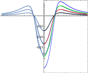
Figure 3. Dipole-type pressure impulses: their induced dimensionless elevations:  $\eta _1(x)$ (dotted), $\eta _2(x)$ (dashed), $\eta _3(x)\vert _{G=0}$. (a) The symmetric case $A=1, B=0$. (b) The antisymmetric case $A=0, B=1$. (c) An asymmetric case $A=B=1$. (d) Gravitational contributions $\eta _3/G$ for $A=1, B=0$ (symmetric) and $A=0, B=1$ (antisymmetric).
7. The 2-D symmetric quadrupole-type impulse
We turn our attention to quadrupole-type pressure impulses. These are fields with a dominant quadrupole contribution, with a dipole term added for the purpose of minimizing the far-field forcing of the horizontal velocity. This improves the possibilities for comparison with slamming flow, where the far-field free-surface flow is strictly vertical. Our quadrupole-type pressure impulse decays so strongly in space that the horizontal far-field velocity is negligible compared with the vertical far-field velocity. The symmetric pressure impulse field of the quadrupole type is chosen as the following harmonic function
 \begin{equation} p_{-1} (x, z) = P_0 \frac{2-5(z/L)-(x/L)^{2} (z/L)+4(z/L)^{2}-(z/L)^{3}}{2((x/L)^{2}+(z/L-1)^{2})^{2}}, \end{equation}
which is an analytical continuation of the surface pressure impulse
 \begin{equation} P(x) = p_{-1}(x,0) = P_0\frac{1}{((x/L)^{2} + 1)^{2}}, \end{equation}
where  $P_0$ again denotes the maximum pressure impulse. The induced zeroth-order potential is
 \begin{equation} \phi_0(x,z) = - \frac{p_{-1}(x,z)}{\rho} = \frac{P_0}{\rho} \frac{-2+5(z/L)+(x/L)^{2} (z/L)-4(z/L)^{2}+(z/L)^{3}}{2((x/L)^{2}+(z/L-1)^{2})^{2}}, \end{equation}
and it is a symmetric quadrupole potential plus a dipole correction providing a far-field decay as  $(x/L)^{-4}$.
Now we introduce dimensionless variables in the same manner as we did for the dipole impulses above. The following transformations
 \begin{equation} \frac{\rho}{P_0} \phi \rightarrow \phi, \quad \left(\frac{x}{L},\frac{z}{L}\right) \rightarrow (x, z), \quad \frac{P_0}{\rho L^{2}} t \rightarrow t, \end{equation}
replace variables with dimension by dimensionless variables, recalling the dimensionless gravity parameter  $G$, still defined by (5.4) above.
We omit most details of the calculations, being similar to those for the dipole pressure impulse. We first give the dimensionless version of the zeroth-order potential (7.3)
 \begin{equation} \phi_0(x,z) = \frac{-2+5 z + x^{2} z - 4 z^{2}+z^{3}}{2(x^{2}+(z-1)^{2})^{2}} = - f_2(x, z), \end{equation}
leading to the first-order elevation
 \begin{align} \eta_1(x) = \phi_{0z}\vert_{z=0} &= \left(\frac{1}{2}f_1+ 2f_2 - 4 f_3\right)_{z=0}\nonumber\\ &= \frac{\partial}{\partial x}\left(-\frac{1}{2}g_1 - g_2 \right)_{z=0}. \end{align}
The first-order potential is
 \begin{equation} \phi_1(x,0) = - \frac{1}{8(x^{2}+1)^{2}} - \frac{1}{(x^{2}+1)^{3}} = -\frac{1}{8}f_2(x, 0) - f_3(x, 0), \end{equation}
which by analytic extension implies  $\phi _1 (x, z) = - f_2(x,z)/8 - f_3(x,z)$ leading to the second-order elevation
 \begin{align} \eta_2(x) & = \left. \frac{1}{2} (\phi_{1z} - \eta_1 \phi_{0xx} - \eta_1' \phi_{0x}) \right\vert_{z=0}\nonumber\\ & = \left(\frac{7}{32}f_1 + \frac{1}{2}f_2 + \frac{5}{4}f_3 + 4 f_4 + 28 f_5 - 128 f_6 + 96 f_7\right)_{z=0}\nonumber\\ & = \frac{\partial}{\partial x}\left(-\frac{7}{32}g_1 - \frac{5}{16}g_2 - \frac{1}{2}g_3 - g_4 - 4g_5 + 8g_6\right)_{z=0}. \end{align}
Taking this procedure one step further, yields the second-order potential, first defined along the undisturbed surface  $z=0$
$z=0$
 \begin{align} 2 \phi_2 & = - 2 \eta_1 \phi_{1z} - \phi_{0x} \phi_{1x} - \eta_1 \eta_1' \phi_{0x} + \eta_1^{2} \phi_{0xx} - G \eta_1\nonumber\\ & = -\frac{7}{16}f_2 - \frac{11}{4}f_3 - 3f_4 - f_5 + 10f_6 + G\left(-\frac{1}{2}f_1 - 2f_2 + 4f_3\right), \quad z=0, \end{align}
and by analytic extension this dependency of  $\phi _2$ on the functions $f_n,\ (n=1,\ldots .,6)$ holds for all $z\le 0$. From this knowledge we derive the total third-order elevation
 \begin{align} \eta_3(x) &= \left( \frac{33}{128}f_2 + \frac{29}{32}f_3 + \frac{13}{24}f_4 + \frac{11}{3}f_5 +\frac{35}{3}f_6 + 84 f_7 + 728 f_8 \right. \nonumber\\ &\quad - \left.\vphantom{\frac{7}{24}}5248 f_9 + 8256 f_{10} - 3840 f_{11} + G (-f_1 - 4 f_2 -2 f_3 +12 f_4)\right)_{z=0}\nonumber\\ & = \frac{\partial}{\partial x} \left(-\frac{11}{128}g_2 - \frac{1}{4}g_3 - \frac{7}{24}g_4 - \frac{2}{3}g_5 - \frac{5}{3}g_6 - 8g_7 - 56g_8 + 256g_9-192g_{10} \right.\nonumber\\ &\quad + G \left.\vphantom{\frac{7}{24}}( g_{1} +2g_2+2g_3 )\right)_{z=0}. \end{align}
These surface elevations are integrated in  $x$ in order to verify mass balance, according to (3.7).
8. The 2-D asymmetric quadrupole-type impulse
We will now study the full early nonlinear interactions between a symmetric quadrupole-type pressure impulse (with dimensionless amplitude  $A$) and an antisymmetric quadrupole-type pressure impulse (with dimensionless amplitude $B$). This oblique quadrupole-type field has its singularities located in the fictitious apex point with dimensionless position $(x, z) = (0, 1)$ outside the fluid.
As in case of an oblique dipole field, capital subscripts  $A$ and $B$ will refer to the contributions from the symmetric and antisymmetric pressure impulses. Combined or repeated subscripts like $AB$ and $BB$ will refer to higher-order cross-interactions or self-interactions.
The total dimensionless zeroth-order potential at the free surface is then
 \begin{equation} \phi_0(x, 0) = - \frac{A}{(x^{2} +1)^{2}} - \frac{B x}{(x^{2} +1)^{2}} = - A f_2(x, 0) - B g_2(x,0), \end{equation}
and by definition  $\phi _0 = \phi _{0A} + \phi _{0B} = - A f_2 - B g_2$ in the entire half-plane $z \le 0$. The dimensionless surface pressure impulse is $P(x) = -\phi _0(x,0) = (A f_2(x,0) + B g_2(x,0))$.
 \begin{equation} \phi_0(x, 0) = - \frac{A}{(x^{2} +1)^{2}} - \frac{B x}{(x^{2} +1)^{2}} = - A f_2(x, 0) - B g_2(x,0), \end{equation}
where the first-order surface elevation
 \begin{align} \eta_1(x) &= \eta_{1A} + \eta_{1B}, \quad z=0\nonumber\\ & = - A f_{2z} - B g_{2z}, \quad z=0, \end{align}
can be written as
 \begin{equation} \eta_1(x) = A (\tfrac{1}{2}f_1 + 2 f_2 - 4 f_3) + B (g_2-4 g_3), \quad z=0. \end{equation}
From this we derive the first-order potential
 \begin{align} \phi_1 & = -\tfrac{1}{2}(\phi_{0x}^{2}+\phi_{0z}^{2}) = \phi_{1A} + \phi_{1B} + \phi_{1AB}\nonumber\\ & = A^{2}(- \tfrac{1}{8}f_2-f_3) + B^{2} (- \tfrac{1}{2}f_3) + AB(-\tfrac{1}{2}g_3), \end{align}
where the last expression is valid for all  $z \le 0$. There is a non-zero interaction potential $\phi _{1AB} = - g_3/2$, while the similar interaction potential was found to be zero for an oblique dipole-field impulsive pressure.
The induced second-order elevation is
 \begin{align} \eta_2(x) &= \eta_{2A} + \eta_{2B} + \eta_{2AB} \nonumber\\ & = A^{2} (\tfrac{7}{32}f_1 +\tfrac{1}{2}f_2 + \tfrac{5}{4}f_3+4f_4+28f_5-128f_6+96f_7)_{z=0} \nonumber\\ &\quad + B^{2} (\tfrac{3}{32}f_1+\tfrac{3}{16}f_2 + \tfrac{3}{4}f_3+9f_4-84f_5+168f_6-96f_7 )_{z=0}\nonumber\\ &\quad + A B (\tfrac{1}{16}g_2+\tfrac{1}{2}g_3+3g_4+32g_5-200g_6+192g_7)_{z=0}. \end{align}
The second-order potential at the undisturbed surface is
 \begin{align} \phi_{2} &= \tfrac{1}{2}( - 2 \eta_1 \phi_{1z} - \phi_{0x} \phi_{1x} - \eta_1 \eta_1' \phi_{0x} + \eta_1^{2} \phi_{0xx} - G \eta_1)\nonumber\\ &= A^{3} ( -\tfrac{7}{32}f_2 -\tfrac{11}{8}f_3 - \tfrac{3}{2}f_4 - \tfrac{1}{2}f_5 + 5f_6 )\nonumber\\ &\quad + B^{3} (-\tfrac{3}{16}g_3 + \tfrac{3}{8}g_4 +3g_6 )\nonumber\\ &\quad + A^{2} B ( -\tfrac{1}{2} g_3 + 7g_6 )\nonumber\\ &\quad + A B^{2} ( -\tfrac{3}{32}f_2 -\tfrac{11}{16}f_3 - \tfrac{9}{8}f_4 - \tfrac{3}{2}f_5 + f_6 )\nonumber\\ &\quad + G (A(-\tfrac{1}{4}f_1 - f_2 + 2f_3)+B (-\tfrac{1}{2}g_2 + 2g_3 )), \quad z=0. \end{align}
The exact formula for the third-order elevation of an oblique quadrupole-type pressure impulse distribution is
 \begin{align} \eta_3(x)& = \eta_{33} + \eta_{321} + \eta_{3111}\nonumber\\ &= A^{3} ( \tfrac{33}{128}f_2 + \tfrac{29}{32}f_3 + \tfrac{13}{24} f_4 + \tfrac{11}{3} f_5 + \tfrac{35}{3} f_6 + 84 f_7 + 728 f_8 -5248f_9 \nonumber\\ &\quad+ 8256f_{10} - 3840f_{11} )_{z=0} \nonumber\\ &\quad + B^{3}(-\tfrac{7}{128}g_2 - \tfrac{3}{32}g_3 - \tfrac{9}{16}g_4 + \tfrac{1}{2} g_5 + 5 g_6 + 150 g_7 - 2016 g_8 + 6720g_9 \nonumber\\ &\quad -8640g_{10} + 3840g_{11})_{z=0} \nonumber\\ &\quad+ A^{2} B ( - \tfrac{11}{128}g_2 - \tfrac{1}{32}g_3 - \tfrac{9}{16}g_4 + \tfrac{7}{3} g_5 + \tfrac{35}{3}g_6 + 116 g_7 + 1288 g_8 - 11392g_9 \nonumber\\ &\quad+ 21312g_{10} -11520g_{11})_{z=0} \nonumber\\ &\quad+ A B^{2} (\tfrac{35}{128}f_1 + \tfrac{65}{128}f_2 + \tfrac{35}{32}f_3 + \tfrac{29}{16} f_4 + \tfrac{19}{2} f_5 + \tfrac{73}{2} f_6 + 722 f_7 - 8820 f_8 \nonumber\\ & \quad + 25920f_9 - 29376f_{10} + 11520f_{11})_{z=0}\nonumber\\ &\quad+ G ( A ( -\tfrac{10}{3} f_3 + 4f_4 ) + B (- 2g_3 + 4 g_4) )_{z=0}. \end{align}
We have performed the mass balance verifications of these expressions, but omit them in the text. These new consistency checks apply to  $\eta _{2BB}$ and $\eta _{3ABB}$, in addition to $\eta _{1A}$, $\eta _{2AA}$, $\eta _{3AAA}$, already checked in the previous section. The remaining contributions to the surface elevation (up to third order) have trivial mass balances. Equation (8.8) includes the full third-order nonlinear interactions.
Figure 4 illustrates the three different types of quadrupole-type pressure impulse distributions that are contained in the general formulas: the symmetric case, the antisymmetric case and an asymmetric case (with central downward flow). All the first-, second- and third-order elevation components resulting from this family of pressure impulses are illustrated in figure 5. In Part 2, these contributions will be summed up to give the total third-order elevation, to be compared with the second-order elevation according to the Lagrangian description of motion. Comparisons with numerical solutions will also be given.

Figure 4. Quadrupole-type pressure impulses  $P(x)$: the symmetric case where $P(x)=P(-x)$ is represented by $(A=1, B=0)$. The antisymmetric case where $P(x) = - P(-x)$ is represented $(A=0, B=1)$. An asymmetric case $(A=B=1)$ is added.

Figure 5. Quadrupole-type pressure impulses: their induced dimensionless elevations:  $\eta _1(x)$ (dotted), $\eta _2(x)$ (dashed), $\eta _3(x)\vert _{G=0}$. (a) The symmetric case $A=1, B=0$. (b) The antisymmetric case $A=0, B=1$. (c) An asymmetric case $A=B=1$. (d) Gravitational contributions $\eta _3/G$ for $A=1, B=0$ (symmetric) and $A=0, B=1$ (antisymmetric).
9. Numerical results for the nonlinear problem
We will here complement our analytical formulas with numerical simulations for the resulting nonlinear wave motion generated by the pressure impulse.
For the numerical computations performed in this section, we apply a dimension-reduced deep-water model which is derived in detail in Bestehorn, Tyvand & Michelitsch (Reference Bestehorn, Tyvand and Michelitsch2019), for a brief overview see appendix C.
The  $(1+1)$ dimensional system in gravitational units (appendix A) has the form
 \begin{gather} \partial_t u_s = - \partial_x(\tfrac 12 u_s^{2} + \eta) + (\partial_x\eta)\hat D \eta, \end{gather}
 \begin{gather}\partial_t \eta = -\partial_x (\hat D^{-1} u_s -\hat D^{-1}(\eta\hat D u_s) + \eta u_s), \end{gather}
where  $u_s=u(x,z=\eta (x,t),t)$ is the horizontal surface velocity and $\eta (x,t)$ denotes the location of the free surface. For the definition of the fractal operator $\hat D$ and its inverse $\hat D^{-1}$ see appendix C.
To integrate (9.1), (9.2) numerically it is effective to evaluate  $\hat D \eta ,\ \hat D u_s$ and $\hat D^{-1}u_s$ in Fourier space, then perform the products $\eta \hat D u_s$ and $\eta u_s$ in real space and finally compute $\hat D^{-1} (\eta \hat D u_s)$ in Fourier space again. Thus, seven Fourier transforms (three forward and four backward) have to be performed at each time step what is achieved applying standard fast Fourier transforms (Swarztrauber Reference Swarztrauber1982).
The derivatives with respect to  $x$ are approximated with centred differences
 \begin{equation} \partial_x f|_{x_i} \longrightarrow \frac{f_{i+1}-f_{i-1}}{2{\rm \Delta} x} \end{equation}
which ensures the conservation of  $\sum _i f_i$, important for mass conservation of (9.2). Finally, time marching is obtained by an explicit fourth-order Runge–Kutta algorithm Bestehorn (Reference Bestehorn2018).
We performed several runs with a symmetric quadrupole-type pressure impulse which is best suited for numerical investigation because it generates flows that are localized in the sense that they decay quickly towards infinity.
The numerical representation of the initial delta-shaped pressure pulse is resolved to a rectangle according to
 \begin{equation} P(x,t) =
\begin{cases} \displaystyle \dfrac{1}{\delta t}
\dfrac{P_0}{(1+x^{2})^{2}} & \mbox{for}\ 0 \le t \le \delta
t, \\ 0 & \mbox{for}\ \delta t< t.
\end{cases} \end{equation}
\begin{equation} P(x,t) =
\begin{cases} \displaystyle \dfrac{1}{\delta t}
\dfrac{P_0}{(1+x^{2})^{2}} & \mbox{for}\ 0 \le t \le \delta
t, \\ 0 & \mbox{for}\ \delta t< t.
\end{cases} \end{equation}
For the impulse time we take  $\delta t = 20 {\rm \Delta} t$, where ${\rm \Delta} t=3\times 10^{-5}$ is the Runge–Kutta time step. For the spatial discretization, 4048 mesh points are used, giving an accurate representation for the intrinsic time and length scales of the solutions. The initial condition for all runs is $\eta (x,0)=u_s(x,0)=0$.
Figure 6 shows time sequences for three different values of  $p_0$. Since the shape of $\eta$ stays mirror symmetric ( $\eta (x,t)=\eta (-x,t$)) for all times, only half of the layer is plotted. It can be clearly seen how the nonlinearities influence the time evolution of the surface shape if $P_0$ increases.

Figure 6. Snapshots for different times with an initial pressure as (9.4) with  $P_0 = 0.1,\ 0.3, \ 0.5$ (a–c). Dashed lines are computed with the linearized set of (9.1), (9.2), solid lines correspond to fully nonlinear solutions. Nonlinear effects increase with increasing initial pressure and surface amplitude.
Nonlinear effects in wave crests are essentially different from nonlinear effects in wave troughs. This is seen immediately from our small-time expansion, because a sign change of the basic amplitude  $A$ does not affect the second-order elevation but changes the signs of the first- and third-order elevations. We will therefore show results for a negative amplitude of the quadrupole-type distribution of pressure impulse, $P_0 = - 0.225$. For a negative initial pressure, the surface is lifted in the initial phase and then spreads out in the form of a travelling localized wave, see figure 7.

Figure 7. Same as figure 6, but for a negative (sucking) initial pressure  $P_0 = -0.225$.
10. Discussion
We have investigated a nonlinear Cauchy–Poisson problem where the flow is caused entirely by an impulsive surface pressure which puts the initially horizontal surface instantaneously into motion. The force impulse that is delivered to the fluid is converted into a net vertical momentum for each fluid column. Even though the net momentum is vertical, most surface particles will also be put into tangential initial motion, because of the tangential derivative of the surface pressure impulse. Due to inertia, the initial flow continues with its momentum after this instantaneous driving force has been turned off, and the total energy is conserved in this inviscid flow. Even though the net momentum is vertical, there is no net mass transport, which is forbidden by mass conservation with zero net mass flux at infinity.
A small-time expansion of the fully nonlinear free-surface flow has been carried out exactly to third order, for two multipole families of surface pressure impulses. We let  $A$ represent the amplitude of the symmetric contribution to each multipole family of pressure impulses that we consider, while $B$ represents the corresponding antisymmetric contribution. The third-order Eulerian solution gives us an opportunity of seeing in detail how the free-surface flow from an asymmetric pressure impulse deviates from a superposition of symmetric and antisymmetric flows. To the second order in time, these deviations enter the product terms $AB$. To the third order in time, these deviations appears as product terms $A B^{2}$ and $A^{2} B$, but their time window of significance is narrow, as the full numerical solution confirms: there is only a short time span from the time when the third-order flow becomes important, until the whole small-time asymptotics breaks down and we are left with only numerical predictions of the further nonlinear flow evolution.
A symmetric pressure impulse with negative amplitude  $-A$ will not give a mirror image of the nonlinear free-surface flow induced by the positive amplitude $+A$. The second-order elevation has the amplitude $A^{2}$ and does not change sign when the pressure impulse changes sign. As a contrast, the first- and third-order elevations have the amplitudes $A$ and $A^{3}$, changing sign when $A$ changes sign. Important nonlinear effects are therefore revealed by comparing two initial pressure impulses that are equal, apart from having opposite signs.
The influence of gravity on the early free-surface flow is governed by the parameter  $G$ defined as
 \begin{equation} G = \frac{\rho^{2} L^{3} g}{P_0^{2}}, \end{equation}
and alternatively the amplitude of the pressure impulse is measured in gravitational units as
 \begin{equation} \hat{P}_0 = G^{-1/2} = \frac{P_0}{\rho L^{3/2} g^{1/2}}. \end{equation}
The highest value of  $\hat {P}_0$ that produces a reasonably accurate surface peak in the numerical computations is $\hat {P}_0 = 0.5$. The surface will probably break if the pressure impulse is significantly stronger than that.
The present small-time expansion is strictly Eulerian. The higher-order surface deformations are described solely through adding up these vertical elevations  $\eta _n$, not by mixing them with Lagrangian descriptions that include tangential motion of the surface particles. This is an important point in the presence of initial tangential surface motion, and it will be investigated in Part 2 of this work whether a small-time expansion in Lagrangian variables may give a closer approximation to the fully nonlinear process than the present Eulerian description. We will not be able to develop a third-order analytical solution in a Lagrangian small-time expansion, only a second-order solution. The present work operates at the limit of what can be done consistently and exactly analytically for moderately strong nonlinear processes. Highly nonlinear free-surface processes can hardly ever be followed closely analytically. The present nonlinear processes are moderately strong, since two consecutive levels of fully nonlinear interactions are calculated exactly in closed form with a finite number of terms. Our full algebra is huge, but it could be carried out efficiently and systematically by Mathematica. All symmetric contributions to the surface elevation have been shown to obey the constraints of mass balance, which is a very useful check for the algebra.
Longuet-Higgins & Dommermuth (Reference Longuet-Higgins and Dommermuth2001) investigated a fully nonlinear standing oscillation which starts as a Cauchy–Poisson problem with a periodic pressure impulse. Their free-surface flow has the following linearized limit
 \begin{equation} \hat{\eta}(\hat{x},\hat{t}) = C \cos (\hat{x}) \sin (\hat{t}), \end{equation}
expressed in gravitational units. Here,  $C$ is the initial vertical velocity at the initially horizontal free surface. A case that is comparable with our present results is represented by $C=0.5$, where maximal surface deflection occurs at the time $t=1.67$ after the impulsive start. The extremal points at the surface are then approximately $\eta _{max} = 0.67$ at the crest and $\eta _{min} = -0.4$ at the trough. Linear theory would give $\eta _{max} = \vert \eta _{min} \vert = 0.5$ occurring at $t = {\rm \pi}/2 = 1.57$. When $C<0.5$, the surface performs a gentle oscillation with almost periodic time dependence, even though the initial state of a horizontal free surface is not fully recovered.
A direct comparison between our results and those of Longuet-Higgins & Dommermuth (Reference Longuet-Higgins and Dommermuth2001) is not possible because of the incompatible definitions of length units, but our strongest computed pressure impulse  $\hat {P}_0 = 0.5$ seems to be reasonably comparable with their case $C=0.5$. Longuet-Higgins & Dommermuth (Reference Longuet-Higgins and Dommermuth2001) has also computed cases with $C>0.5$, and in these cases slender upward spikes will be formed under a strong impulsive suction (negative pressure impulse). Such upward spikes cannot continue as waves, so they will eventually fall down as slender jet flows with an acceleration close to gravity and inevitably lead to breaking of the free surface.
More general conclusions concerning the present model and its three solution methods will be presented at the end of Part 2.
Declaration of interests
The authors report no conflict of interest.
Appendix A. Gravitational dimensionless variables
In the main text we have introduced and applied dimensionless variables based on the amplitude of the pressure impulse, which is convenient for the early nonlinear process where gravity does not enter the second-order problem. However, the process will become gravitational after this early stage, so we need gravitational units for describing the gravitational free-surface flow that takes over after the early impulsive stage is finished.
We will now introduce dimensionless variables based on gravity, noting that  $L$ is the only length scale. With infinite depth, $L$ must still be chosen as the length scale of the pressure impulse. The mathematical apex point for the dipole field is thus located one length unit above the undisturbed free surface. We choose gravitational units for the flow, which means that we informally can introduce all the dimensionless units by putting $g=1,~L=1$ and $\rho =1$.
The formal introduction of dimensionless variables in gravitational units can be given as follows
 \begin{gather} \frac{(x, y, z)}{L} = (\tilde{x},\tilde{y}, \tilde{z}), \quad L \boldsymbol{\nabla} = \tilde{\boldsymbol{\nabla}}, \quad L^{-1} \eta = \tilde{\eta}, \quad \sqrt{\frac{g}{L}} t = \tilde{t}, \end{gather}
 \begin{gather}\frac{(u, v, w)}{\sqrt{gL}} = (\tilde{u},\tilde{v}, \tilde{w}), \quad (g L^{3})^{-1/2} \varPhi = \tilde{\varPhi}, \quad \frac{p}{\rho g L} = \tilde{p}, \quad \frac{P}{\rho g^{1/2} L^{3/2}} = \tilde{P}, \end{gather}
where the dimensionless quantities are represented by a tilde superscript. In the main text we have worked with dimensionless quantities based on the pressure impulse amplitude  $P_0$, which generates unit flow amplitudes in this dimensionless description, and gravity enters the problem through a dimensionless gravity parameter
 \begin{equation} G = \frac{\rho^{2} L^{3}}{P_0^{2}} g, \end{equation}
scaled with the amplitude and length scale of the pressure impulse. With gravitational units for dimensionless variables, the gravitational parameter will always be unity, making the substitution  $G \rightarrow 1$ in the equations of the main text. With gravitational variables, the flow amplitude will no longer be unity but instead given by the initial condition
 \begin{equation} {-}\rho \phi(x,y,0) = P(x,y), \end{equation}
which has the dimensionless version
 \begin{equation} {-}\tilde{\phi}(\tilde{x},\tilde{y},0) = \tilde{P}(\tilde{x},\tilde{y}) = \frac{P(x,y)}{\rho (g L^{3})^{1/2}}. \end{equation}
The dimensionless amplitude of the pressure impulse is thus given by
 \begin{equation} \tilde{P}_0 = \frac{P_0}{\rho (g L^{3})^{1/2}} = \frac{1}{\sqrt{G}}, \end{equation}
which now represents the initial flow amplitude of the dimensionless zeroth-order potential  $\tilde {\phi }_0$ in the small-time expansion. We note the relationship between $\tilde {P}_0$ and the dimensionless gravity parameter $G$ which was used in the main text.
Appendix B. Two families of harmonic functions
We will here develop recursive schemes for calculating the requested higher orders of the harmonic functions  $f_n(x,z)$ and $g_n(x,z)$ defined by their values at the boundary of the half-plane $z<0$
$z<0$
 \begin{gather} f_n(x,0) = \frac{1}{(1+x^{2})^{n}}, \end{gather}
 \begin{gather}g_n(x,0) = \frac{x}{(1+x^{2})^{n}}, \end{gather}
where  $n$ is a positive integer. These functions are here presented in dimensionless form.
We note the useful identities
 \begin{gather} f_m (x, 0) f_n (x, 0) = f_{m+n} (x, 0), \end{gather}
 \begin{gather}g_m (x, 0) f_n (x, 0) = g_{m+n} (x, 0), \end{gather}
 \begin{gather}g_m (x, 0) g_n (x, 0) = f_{m+n-1} (x, 0) - f_{m+n} (x, 0). \end{gather}
We will now show how these related families of multipole-type functions can be calculated recursively. First, we introduce a source potential  $\chi$ in the apex point $(0,1)$, which is a fictitious point located outside the fluid domain,
 \begin{equation} \chi = \tfrac{1}{2} \log(x^{2} + (z-1)^{2}) \end{equation}
and its gradients give us the two first-order functions
 \begin{gather} f_1(x,z) = - \frac{\partial \chi}{\partial z} = \frac{1-z}{x^{2} + (z-1)^{2}}, \end{gather}
 \begin{gather}g_1(x,z) = \frac{\partial \chi}{\partial x} = \frac{x}{x^{2} + (z-1)^{2}}. \end{gather}
Each new order function is a linear combination of the  $z$ derivative of the previous function plus a linear combination of the lower-order function, according to the following recursive scheme
 \begin{gather} 2 f_2 = f_1 + \frac{\partial f_1}{\partial z}, \end{gather}
 \begin{gather}2 g_2 = \frac{\partial g_1}{\partial z}, \end{gather}
 \begin{gather}4 f_3 = \frac{1}{2} f_1 + 2 f_2 + \frac{\partial f_2}{\partial z}, \end{gather}
 \begin{gather}4 g_3 = g_2 + \frac{\partial g_2}{\partial z}, \end{gather}
 \begin{gather}6 f_4 = \frac{3}{8} f_1 + \frac{3}{4} f_2 + 3 f_3 +\frac{\partial f_3}{\partial z}, \end{gather}
 \begin{gather}6 g_4 = \frac{1}{4} g_2 + 2 g_3 + \frac{\partial g_3}{\partial z}, \end{gather}
 \begin{gather}8 f_5 = \frac{5}{16} f_1 + \frac{1}{2} f_2 + f_3 + 4 f_4 + \frac{\partial f_4}{\partial z}, \end{gather}
 \begin{gather}8 g_5 = \frac{1}{8} g_2 + \frac{1}{2} g_3 + 3 g_4 + \frac{\partial g_4}{\partial z}, \end{gather}
 \begin{gather}10 f_6 = \frac{35}{128} f_1 + \frac{25}{64} f_2 + \frac{5}{8} f_3 + \frac{5}{4} f_4 + 5 f_5 + \frac{\partial f_5}{\partial z}, \end{gather}
 \begin{gather}10 g_6 = \frac{5}{64} g_2 + \frac{1}{4} g_3 + \frac{3}{4} g_4 + 4 g_5 + \frac{\partial g_5}{\partial z}, \end{gather}
 \begin{gather}12 f_7 = \frac{63}{256} f_1 + \frac{21}{64} f_2 + \frac{15}{32} f_3 + \frac{3}{4} f_4 + \frac{3}{2} f_5 + 6 f_6 +\frac{\partial f_6}{\partial z}, \end{gather}
 \begin{gather}12 g_7 = \frac{7}{128} g_2 + \frac{5}{32} g_3 + \frac{3}{8} g_4 + g_5 + 5 g_6 + \frac{\partial g_6}{\partial z}, \end{gather}
 \begin{gather}14 f_8 = \frac{231}{1024} f_1 + \frac{147}{512} f_2 + \frac{49}{128} f_3 + \frac{35}{64} f_4 + \frac{7}{8} f_5 + \frac{7}{4} f_6 + 7 f_7 + \frac{\partial f_7}{\partial z}, \end{gather}
 \begin{gather}14 g_8 = \frac{21}{512} g_2 + \frac{7}{64} g_3 + \frac{15}{64} g_4 + \frac{1}{2} g_5 + \frac{5}{4} g_6 + 6 g_7 + \frac{\partial g_7}{\partial z}, \end{gather}
 \begin{gather}16 f_9 = \frac{429}{2048} f_1 + \frac{33}{128} f_2 + \frac{21}{64} f_3 + \frac{7}{16} f_4 + \frac{5}{8} f_5 + f_6 + 2 f_7 + 8 f_8 + \frac{\partial f_8}{\partial z}, \end{gather}
 \begin{gather}16 g_9 = \frac{33}{1024} g_2 + \frac{21}{256} g_3 + \frac{21}{128} g_4 + \frac{5}{16} g_5 + \frac{5}{8} g_6 + \frac{3}{2} g_7 + 7 g_8 + \frac{\partial g_8}{\partial z}, \\\nonumber\end{gather}
 \begin{align} 18 f_{10} &= \frac{6435}{32768} f_1 + \frac{3861}{16384} f_2 + \frac{297}{1024} f_3 + \frac{189}{512} f_4 + \frac{63}{128} f_5 + \frac{45}{64} f_6 + \frac{9}{8} f_7 \nonumber\\ &\quad + \frac{9}{4} f_8 + 9 f_9 + \frac{\partial f_9}{\partial z}, \end{align}
 \begin{align} 18 g_{10} &= \frac{429}{16384} g_2 + \frac{33}{512} g_3 + \frac{63}{512} g_4 + \frac{7}{32} g_5 + \frac{25}{64} g_6 + \frac{3}{4} g_7 + \frac{7}{4} g_8 + 8 g_9 + \frac{\partial g_9}{\partial z},\\ 20 f_{11} &= \frac{12155}{65536} f_1 + \frac{3575}{16384} f_2 + \frac{2145}{8192} f_3 + \frac{165}{512} f_4 + \frac{105}{256} f_5 + \frac{35}{64} f_6 + \frac{25}{32} f_7 \nonumber\\ &\quad + \frac{5}{4} f_8 + \frac{5}{2} f_9 + 10 f_{10}+ \frac{\partial f_{10}}{\partial z}, \end{align}
 \begin{align} 20 g_{11} &= \frac{715}{32768} g_2 + \frac{429}{8192} g_3 + \frac{99}{1024} g_4 + \frac{21}{128} g_5 + \frac{35}{128} g_6 \nonumber\\ &\quad + \frac{15}{32} g_7 + \frac{7}{8} g_8 + 2 g_9 + 9 g_{10}+ \frac{\partial g_{10}}{\partial z}. \end{align}
Note that these recursive formulas are valid in the entire half-plane  $z \le 0$.
In the free-surface conditions we need the first and second derivatives of these functions, to be expressed by the values of the functions at the undisturbed free surface,  $f_n(x,0)$ and $g_n(x,0)$. The recursion formulas that we have developed here, contain the information for calculating these derivatives. We will now list the coefficients entering the expressions for the vertical derivatives at the undisturbed free surface, defined by
 \begin{equation} \left.\frac{\partial f_n}{\partial z}\right\vert_{z=0} = \sum_{j=1}^{j=n+1} A_{nj} f_j(x,0), \quad \left. \frac{\partial g_n}{\partial z}\right\vert_{z=0} = \sum_{j=2}^{j=n+1} B_{nj} g_j(x,0), \end{equation}
where  $n = 1, 2,\ldots$. The increasing-order sets of coefficients for the vertical derivatives of the functions $f_n$ are
 \begin{gather} (A_{11}, A_{12}) = (-1, 2), \end{gather}
 \begin{gather}(A_{21}, A_{22}, A_{23}) = (-\tfrac{1}{2}, -2, 4), \end{gather}
 \begin{gather}(A_{31}, A_{32}, A_{33}, A_{34}) = (-\tfrac{3}{8},-\tfrac{3}{4}, -3, 6), \end{gather}
 \begin{gather}(A_{41}, A_{42}, A_{43}, A_{44}, A_{45}) = (-\tfrac{5}{16},-\tfrac{1}{2}, -1, -4, 8), \end{gather}
 \begin{gather}(A_{51}, A_{52}, A_{53}, A_{54}, A_{55}, A_{56}) = (-\tfrac{35}{128},-\tfrac{25}{64}, -\tfrac{5}{8}, -\tfrac{5}{4}, -5, 10), \end{gather}
 \begin{gather}(A_{61}, A_{62}, A_{63}, A_{64}, A_{65}, A_{66}, A_{67}) = (-\tfrac{63}{256}, -\tfrac{21}{64}, -\tfrac{15}{32}, -\tfrac{3}{4}, -\tfrac{3}{2}, -6, 12), \nonumber \end{gather}
 \begin{gather} (A_{71}, A_{72}, A_{73}, A_{74}, A_{75}, A_{76}, A_{77}, A_{78}) = (-\tfrac{231}{1024}, -\tfrac{147}{512}, -\tfrac{49}{128}, -\tfrac{35}{64}, -\tfrac{7}{8}, -\tfrac{7}{4}, -7, 14), \end{gather}
 \begin{align} &(A_{81}, A_{82}, A_{83}, A_{84}, A_{85}, A_{86}, A_{87}, A_{88}, A_{89})\nonumber\\ &\quad = (-\tfrac{429}{2048}, -\tfrac{33}{128}, -\tfrac{21}{64}, -\tfrac{7}{16}, -\tfrac{5}{8}, - 1, - 2, -8, 16), \end{align}
 \begin{align} &(A_{91}, A_{92}, A_{93}, A_{94}, A_{95}, A_{96}, A_{97}, A_{98}, A_{99}, A_{9,10})\nonumber\\ &\quad = (-\tfrac{6435}{32768}, -\tfrac{3861}{16384}, -\tfrac{297}{1024}, -\tfrac{189}{512}, -\tfrac{63}{128}, -\tfrac{45}{64}, -\tfrac{9}{8}, -\tfrac{9}{4}, - 9 , 18),\end{align}
 \begin{align} &(A_{101}, A_{102}, A_{103}, A_{104}, A_{105}, A_{106}, A_{107}, A_{108}, A_{109}, A_{10,10}, A_{10,11}) \notag\\ &\quad =(-\tfrac{12155}{65536}, -\tfrac{3575}{16384}, -\tfrac{2145}{8192}, -\tfrac{165}{512}, -\tfrac{105}{256}, -\tfrac{35}{64}, -\tfrac{25}{32}, -\tfrac{5}{4}, -\tfrac{5}{2}, - 10 , 20). \end{align}
The increasing-order sets of non-zero coefficients for the vertical derivatives of the functions  $g_n$ are
 \begin{gather} B_{12} = 2, \end{gather}
 \begin{gather}(B_{22}, B_{23}) = (-1, 4), \end{gather}
 \begin{gather}(B_{32}, B_{33}, B_{34}) = (-\tfrac{1}{4},-2, 6 ), \end{gather}
 \begin{gather}(B_{42}, B_{43}, B_{44}, B_{45}) = (-\tfrac{1}{8},-\tfrac{1}{2}, -3, 8), \end{gather}
 \begin{gather}(B_{52}, B_{53}, B_{54}, B_{55}, B_{56}) = (-\tfrac{5}{64},-\tfrac{1}{4}, -\tfrac{3}{4}, -4, 10), \end{gather}
 \begin{gather}(B_{62}, B_{63}, B_{64}, B_{65}, B_{66}, B_{67}) = (-\tfrac{7}{128}, -\tfrac{5}{32}, -\tfrac{3}{8}, -1, -5, 12), \end{gather}
 \begin{gather}(B_{72}, B_{73}, B_{74}, B_{75}, B_{76}, B_{77}, B_{78}) = (-\tfrac{21}{512}, -\tfrac{7}{64}, -\tfrac{15}{64}, -\tfrac{1}{2}, -\tfrac{5}{4}, - 6, 14), \\[-3pc]\nonumber\end{gather}
 \begin{align} &(B_{82}, B_{83}, B_{84}, B_{85}, B_{86}, B_{87}, B_{88}, B_{89})\nonumber\\ &\quad = (-\tfrac{33}{1024}, -\tfrac{21}{256}, -\tfrac{21}{128}, -\tfrac{5}{16}, -\tfrac{5}{8}, -\tfrac{3}{2} , - 7, 16), \end{align}
 \begin{align} &(B_{92}, B_{93}, B_{94}, B_{95}, B_{96}, B_{97}, B_{98}, B_{99}, B_{9,10})\nonumber\\ &\quad = (-\tfrac{429}{16384}, -\tfrac{33}{512}, -\tfrac{63}{512}, -\tfrac{7}{32}, -\tfrac{25}{64}, -\tfrac{3}{4}, - \tfrac{7}{4}, - 8, 18), \end{align}
 \begin{align} &(B_{102}, B_{103}, B_{104}, B_{105}, B_{106}, B_{107}, B_{108}, B_{109}, B_{10,10}, B_{10,11})\nonumber\\ &\quad = (-\tfrac{715}{32768}, -\tfrac{429}{8192}, -\tfrac{99}{1024}, -\tfrac{21}{128}, -\tfrac{35}{128}, -\tfrac{15}{32}, - \tfrac{7}{8}, - 2, -9, 20). \end{align}
The relationships for the horizontal derivatives of these functions can be written by general formulas (valid for all positive integers  $n$)
$n$)
 \begin{gather} \left.\frac{\partial f_n}{\partial x}\right\vert_{z=0} = -2 n g_{n+1}(x,0), \end{gather}
 \begin{gather}\left.\frac{\partial g_n}{\partial x}\right\vert_{z=0} = (1 - 2 n) f_n(x,0) + 2 n f_{n+1}(x,0), \end{gather}
 \begin{gather}\left.\frac{\partial^{2} f_n}{\partial x^{2}}\right\vert_{z=0} = 2 n (2 n + 1) f_{n+1}(x,0) - 4 n (n+1)f_{n+2}(x,0) = - \left. \frac{\partial^{2} f_n}{\partial z^{2}}\right\vert_{z=0} , \end{gather}
 \begin{gather}\left.\frac{\partial^{2} g_n}{\partial x^{2}}\right\vert_{z=0} = 2 n (2 n - 1) g_{n+1}(x,0) - 4 n (n + 1) g_{n+2}(x,0) = - \left. \frac{\partial^{2} g_n}{\partial z^{2}}\right\vert_{z=0} , \end{gather}
where Laplace's equation has been utilized.
Appendix C. Dimension-reduced deep-water model
We give a brief derivation for the dimension-reduced deep-water model (9.1), (9.2) applied for the numerical computations of § 9. For more details see Bestehorn et al. (Reference Bestehorn, Tyvand and Michelitsch2019).
Starting from the kinematic boundary condition and the Euler equations for an incompressible, potential flow, the set
 \begin{equation} \left.\begin{array}{c}
\partial_t u_s = - \left.\dfrac 12\partial_x( u_s)^{2}
-\dfrac{1}{\rho}\partial_x p \right|_{z=\eta},
\\ \partial_t \eta = -\partial_x S,
\end{array}\right\} \end{equation}
\begin{equation} \left.\begin{array}{c}
\partial_t u_s = - \left.\dfrac 12\partial_x( u_s)^{2}
-\dfrac{1}{\rho}\partial_x p \right|_{z=\eta},
\\ \partial_t \eta = -\partial_x S,
\end{array}\right\} \end{equation}
is found where  $u_s(x,t) = u(x,z=\eta (x,t),t)$ is the horizontal velocity component at the free surface located at $z=\eta (x,t)$ and
 \begin{equation} S(x,t) = \int_{-\infty}^{\eta(x,t)} \, \textrm{d} z u(x,z,t), \end{equation}
denotes the horizontal flux. From  $\nabla ^{2} u = 0$, the general form for $u$ reads
 \begin{equation} u = \sum_k u_k(t) \mbox{e}^{|k|z} \,\mbox{e}^{\textrm{i} k x} + \textrm{c.c.}, \end{equation}
and therefore
 \begin{equation} S(x,t) = \sum_k \frac{\mbox{e}^{|k|\eta(x,t)}}{|k|} u_k(t)\,\mbox{e}^{\textrm{i} k x} + \textrm{c.c.}, \end{equation}
where c.c. stands for complex conjugate. Expanding e $^{|k|\eta }$ with respect to the (small) steepness $s=|k|\eta$ (C 3) is written as
 \begin{equation} u_s = \sum_k u_k(t)\sum_{n=0}^{N}\frac{(|k|\eta)^{n}}{n!} \,\mbox{e}^{\textrm{i} k x} + \textrm{c.c.} \end{equation}
We define the linear fractional operator of order  $s^{N}$
 \begin{equation} \hat L_N(\eta) = \sum_{n=0}^{N}\frac{\eta^{n}\hat D^{n}}{n!}, \end{equation}
with  $\hat D$ as the self-adjoint operator
 \begin{equation} \hat D \equiv (-\partial_{xx})^{1/2}, \end{equation}
that has the Fourier representation  $\hat D^{n} \longrightarrow |k|^{n}$. Now, $u_k$ can be eliminated between (C 4), (C 5) and up to order $s^{N}$ (C 2) takes the form
 \begin{equation} S_N(x,t) = \hat L_N(\eta) \hat D^{-1} \hat L_N^{-1}(\eta) u_s(x,t), \end{equation}
with  $\hat L_N^{-1}$ as operator inverse constructed from
 \begin{equation} \hat L_N^{-1} \hat L_N = 1 + O(\eta^{N+1}). \end{equation}
Up to first order ( $N=1$), (C 6) and (C 9) yield
 \begin{equation} \hat L_1 = 1 + \eta\hat D, \quad \hat L_1^{-1} = 1 - \eta\hat D , \end{equation}
and (C 8) explicitly reads
 \begin{equation} S_1 = \hat D^{-1} u_s -\hat D^{-1}(\eta\hat D u_s) + \eta u_s . \end{equation}
Assuming for the surface pressure  $p(x, z=\eta (x)) = \textrm {const.}$, the pressure gradient in (C 1) reads $\partial _x p|_{z=\eta } = -\partial _z p|_{z=\eta }\partial _x\eta$ and with the Euler equation (first order)
 \begin{equation} \partial_z p|_{z=\eta} = \rho (g +\partial_t w_s)\partial_x \eta . \end{equation}
Here,  $w_s(x,t) = w(x, z=\eta (x,t),t)$ denotes the vertical velocity component at the surface and can be taken from the continuity equation in appropriate order as $w_s = -\partial _x \hat D^{-1} u_s$. Finally, (C 1) turns into
 \begin{equation} [1-(\partial_x\eta)\partial_x\hat D^{-1}]\partial_t u_s = - \partial_x(\tfrac 12 u_s^{2} + g \eta). \end{equation}
Inversion of the operator in the brackets on the left-hand side of (C 13) and scaling according to appendix A, (9.1) and (9.2) are obtained in the desired second order  $s^{2}$.


 Open access