2. Formulation of the mathematical model

We consider an inviscid and incompressible fluid which has initially a horizontal free surface $z=0$. The fluid (liquid) has a free surface subject to constant atmospheric pressure $p_{atm}$. Cartesian coordinates $x, y, z$ are introduced, where the $z$ axis is directed upwards in the gravity field and the horizontal $x, y$ plane defines the undisturbed free surface. The gravitational acceleration is ${\boldsymbol {g}}$, and $\rho$ denotes the constant fluid density. The undisturbed fluid is initially at rest with a horizontal free surface $z=0$. See the definition sketch in the previous paper (Part 1).

The nonlinear free-surface flow will be described by the Lagrangian description of motion, whereby we define the flow variables

(2.1a–c)\begin{equation} x = x(a,b,c,t),\quad y = y(a,b,c,t),\quad z = z(a,b,c,t), \end{equation}

with the corresponding representation of the pressure field

(2.2)\begin{equation} p = p(a,b,c,t). \end{equation}

Equations (2.1a–c) and (2.2) constitute the Lagrangian description of motion, with independent Lagrangian variables $(a,b,c)$ following individual particles in their motion, while time is denoted by $t$. We restrict the analysis to semi-infinite fluid domains, with vanishing flow as $z \rightarrow - \infty$. The free-surface flow vanishes as $c \rightarrow - \infty$ in Lagrangian variables.

Our Lagrangian description of motion follows Lamb (Reference Lamb1932). We identify the Lagrangian variables $(a,b,c)$ with the position before the motion starts at $t=0$

(2.3)\begin{equation} a = x(a,b,c,t),\quad b = y(a,b,c,t),\quad c = z(a,b,c,t),\quad t \le 0. \end{equation}

Hereby, the free surface is defined by $c=0$ at all times. The Lagrangian continuity equation is

(2.4)\begin{equation} \frac{\partial(x,y,z)}{\partial(a,b,c)} = 1. \end{equation}

The components of the equation of motion are

(2.5)\begin{gather} \frac{\partial^2 x}{\partial t^2} \frac{\partial x}{\partial a} + \frac{\partial^2 y}{\partial t^2} \frac{\partial y}{\partial a} + \left(\frac{\partial^2 z}{\partial t^2} + g \right) \frac{\partial z}{\partial a} + \frac{1}{\rho} \frac{\partial p}{\partial a} = 0, \end{gather}

(2.6)\begin{gather}\frac{\partial^2 x}{\partial t^2} \frac{\partial x}{\partial b} + \frac{\partial^2 y}{\partial t^2} \frac{\partial y}{\partial b} + \left(\frac{\partial^2 z}{\partial t^2} + g \right) \frac{\partial z}{\partial b} + \frac{1}{\rho} \frac{\partial p}{\partial b} = 0, \end{gather}

(2.7)\begin{gather}\frac{\partial^2 x}{\partial t^2} \frac{\partial x}{\partial c} + \frac{\partial^2 y}{\partial t^2} \frac{\partial y}{\partial c} + \left(\frac{\partial^2 z}{\partial t^2} + g \right) \frac{\partial z}{\partial c} + \frac{1}{\rho} \frac{\partial p}{\partial c} = 0. \end{gather}

The nonlinear dynamic free-surface condition is

(2.8a,b)\begin{equation} \frac{\partial p}{\partial a} = \frac{\partial p}{\partial b} = 0,\quad c=0, \end{equation}

expressing constant (atmospheric) pressure along the free surface $c=0$.

3. The small-time expansion

The motionless fluid is forced impulsively into motion at $t=0$, giving the relationships

(3.1)\begin{gather} x(a,b,c,t) = a + H(t)(x_1(a,b,c) t + x_2(a,b,c) t^2 +\cdots) , \end{gather}

(3.2)\begin{gather}y(a,b,c,t) = b + H(t)(y_1(a,b,c) t + y_2(a,b,c) t^2 +\cdots) , \end{gather}

(3.3)\begin{gather}z(a,b,c,t) = c + H(t)(z_1(a,b,c) t + z_2(a,b,c) t^2 +\cdots) , \end{gather}

valid for small time after the impulsive forcing during the infinitesimal time interval $0<t<0^+$. Here, $H(t)$ is the Heaviside unit step function. The small-time expansion for the liquid pressure is

(3.4)\begin{equation} p(a,b,c,t) = -\rho g c + \delta(t) p_{-1}(a,b,c) + H(t)(p_0(a,b,c) + p_1(a,b,c) t +\cdots), \end{equation}

where $\delta (t)$ denotes Dirac's delta function. Surface tension is neglected, and the pressure is measured relative to the atmospheric pressure. Pohle (Reference Pohle1952) performed an early Lagrangian small-time expansion of dam breaking, expanding the flow to second order. Since his work covers only linear theory, it is not comparable with our nonlinear theory.

3.1. The first-order problem

We will first derive the boundary value problem to the leading order. It is linearized description, corresponding to the leading-order Eulerian description of our preceding paper (Part 1). The leading-order flow is determined by integrating the equation of motion over the infinitesimal interval of impulsive start, determining the net pressure impulse $P(a,b,0)$ applied to the surface

(3.5)\begin{equation} P(a,b) = \int_0^{0^+} p(a,b,0,t) \,\textrm{d}t = p_{-1} (a,b,0), \end{equation}

applying (3.4). The same integrating in time of the equation of motion gives

(3.6a–c)\begin{equation} x_1 + \frac{1}{\rho} \frac{\partial p_{-1}}{\partial a} = 0,\quad y_1 + \frac{1}{\rho} \frac{\partial p_{-1}}{\partial b} = 0,\quad z_1 + \frac{1}{\rho} \frac{\partial p_{-1}}{\partial c} = 0, \end{equation}

to be evaluated at the surface for specifying the dynamic initial conditions

(3.7a,b)\begin{equation} x_1(a,b,0) + \frac{1}{\rho} \frac{\partial P}{\partial a} = 0,\quad y_1(a,b,0) + \frac{1}{\rho} \frac{\partial P}{\partial b} = 0. \end{equation}

Lord Kelvin's circulation theorem requires that the initial flow has zero vorticity, which gives

(3.8a–c)\begin{equation} \frac{\partial x_1}{\partial b} - \frac{\partial y_1}{\partial a} = 0,\quad \frac{\partial y_1}{\partial c} - \frac{\partial z_1}{\partial b} = 0,\quad \frac{\partial z_1}{\partial a} - \frac{\partial x_1}{\partial c} = 0, \end{equation}

and it follows that the initial velocity is the gradient of a potential $\phi _1(a,b,c)$

(3.9)\begin{equation} (x_1, y_1, z_1) = \boldsymbol{\nabla}_L \phi_1, \end{equation}

introducing the Lagrangian gradient operator $\boldsymbol {\nabla }_L$ by its components

(3.10)\begin{equation} \boldsymbol{\nabla}_L = \left(\frac{\partial}{\partial a}, \frac{\partial}{\partial b}, \frac{\partial}{\partial c} \right). \end{equation}

The first-order continuity equation follows from the time derivative of (2.4)

(3.11)\begin{equation} \frac{\partial x_1}{\partial a} + \frac{\partial y_1}{\partial b} + \frac{\partial z_1}{\partial c} = 0. \end{equation}

Inserting (3.9) into (3.11) leads to Laplace's equation in Lagrangian coordinates

(3.12)\begin{equation} {\nabla}_L^2 \phi_1 = 0. \end{equation}

Integrating each horizontal component of the equation of motion (3.6a–c) gives

(3.13)\begin{equation} \phi_1 = - \frac{p_{-1}}{\rho}. \end{equation}

This relationship is valid in the entire fluid domain. The surface condition is

(3.14)\begin{equation} \phi_1(a,b,0) = - \frac{P(a,b)}{\rho} = - \frac{p_{-1}(a,b,0)}{\rho}, \end{equation}

and we extend analytically this surface pressure impulse $P(a,b)$ as a harmonic function $p_{-1}(a,b,c)$.

3.2. The second-order problem

The second-order problem follows from the equation of motion (2.5)–(2.7). Inserting the small-time expansion and putting $t=0$ produces the gradient relationship

(3.15)\begin{equation} (x_2, y_2, z_2) = - \frac{1}{2 \rho} \boldsymbol{\nabla}_L p_0 = \boldsymbol{\nabla}_L \phi_2, \end{equation}

introducing a second-order potential $\phi _2(a, b, c)$. The governing equation for the second-order potential is found from the continuity equation (2.4), differentiated twice in time, yielding

(3.16)\begin{equation} {\nabla}_L^2 \phi_2 = \frac{\partial x_1}{\partial c} \frac{\partial z_1}{\partial a} + \frac{\partial y_1}{\partial a} \frac{\partial x_1}{\partial b} + \frac{\partial z_1}{\partial b} \frac{\partial y_1}{\partial c} - \frac{\partial x_1}{\partial a} \frac{\partial z_1}{\partial c} - \frac{\partial y_1}{\partial b} \frac{\partial x_1}{\partial a} - \frac{\partial z_1}{\partial c} \frac{\partial y_1}{\partial b}, \end{equation}

after inserting the small-time expansion and put $t=0$. This governing equation is rewritten as

(3.17)\begin{align} {\nabla}_L^2 \phi_2 = \left(\frac{\partial^2 \phi_1}{\partial a \partial b}\right)^2 + \left(\frac{\partial^2 \phi_1}{\partial b \partial c}\right)^2 + \left(\frac{\partial^2 \phi_1}{\partial c \partial a}\right)^2 - \frac{\partial^2 \phi_1}{\partial a^2} \frac{\partial^2 \phi_1}{\partial b^2} - \frac{\partial^2 \phi_1}{\partial b^2} \frac{\partial^2 \phi_1}{\partial c^2} - \frac{\partial^2 \phi_1}{\partial c^2} \frac{\partial^2 \phi_1}{\partial a^2}. \end{align}

The right-hand side corrects to second order a mass defect induced by the first-order terms. This is Poisson's equation ${\nabla }_L^2 \phi _2 = Q(a,b,c)$, with a source distribution $Q(a,b,c)$. The only boundary conditions (with infinite depth) are the two components of the dynamic condition (2.8a,b). Combined with the equation of motion, the dynamic conditions emerge

(3.18a,b)\begin{equation} x_2 = y_2 = 0,\quad c=0, \end{equation}

whereby we arrive at a single dynamic equipotential condition

(3.19a,b)\begin{equation} \phi_2 = 0,\quad c=0. \end{equation}

This dynamic free-surface condition is a condition of antisymmetry around $c=0$,

(3.20)\begin{equation} \phi_2(a, b, c) = - \phi_2(a, b, -c). \end{equation}

This completes our second-order formulation in three dimensions.

Our Lagrangian small-time expansion is carried out to second order, where there is no influence from gravity. Our preceding paper (Part 1) gives analytical and numerical results concerning the related gravitational problem of oscillatory waves. Gravity is important at the gravitational time scale, which is a large time scale for a strong pressure impulse. A strong suction impulse (upward) will induce surface breaking when the flow becomes gravitational (Longuet-Higgins & Dommermuth Reference Longuet-Higgins and Dommermuth2001).

3.3. Solution procedure for the second-order problem

From now on we work with two-dimensional (2-D) flow in the $x, z$ plane, proceeding in parallel with our 2-D Eulerian theory for the same problem (Part 1), where we applied a third-order small-time expansion. We will consider 2-D dipole and quadrupole distributions for the pressure impulse. We take the following transformations from variables with dimension to non-dimensional variables

(3.21a,b)\begin{equation} \left(\frac{a}{L}, \frac{c}{L}\right) \rightarrow (a, c),\quad \frac{P_0}{\rho L^2} t \rightarrow t, \end{equation}

where $L$ is the length scale of the pressure impulse, and $P_0$ is its amplitude. To the present order of approximation, the omission of the density $\rho$ is the only visible change when the description becomes dimensionless. Our preceding paper (Part 1, appendix A) introduces an alternative set of gravitational dimensionless variables as a second option.

The governing equation (3.17) in its 2-D version reduces to

(3.22)\begin{equation} {\nabla}_L^2 \phi_2 = \left(\frac{\partial^2 \phi_1}{\partial a \partial c}\right)^2 - \frac{\partial^2 \phi_1}{\partial a^2} \frac{\partial^2 \phi_1}{\partial c^2} = \left(\frac{\partial^2 \phi_1}{\partial a \partial c}\right)^2 + \left(\frac{\partial^2 \phi_1}{\partial a^2}\right)^2,\quad c<0, \end{equation}

applying Laplace's equation. By the dynamic condition (3.20), we extend the governing equation

(3.23)\begin{equation} {\nabla}_L^2 \phi_2 = - \mbox{sign}(c) \left( \left(\frac{\partial^2 \phi_1}{\partial a \partial c}\right)^2 + \left(\frac{\partial^2 \phi_1}{\partial a^2}\right)^2 \right) = q(a,c), \end{equation}

to the entire $a, c$ plane by the source distribution $q(a,c)$. It is similar to a distribution of free charges in electrostatics. Mass balance to second order is achieved by the Green's function integral

(3.24)\begin{equation} \phi_2(a, c) = \frac{1}{4 {\rm \pi}} \int_{-\infty}^{\infty} \int_{-\infty}^{\infty} q(a', c') \log ((a-a')^2 + (c-c')^2) \,\textrm{d}a' \,\textrm{d}c'. \end{equation}

4. Oblique dipole-type pressure impulse

As in our previous paper (Part 1) we define the multipole-type 2-D harmonic functions

(4.1)\begin{gather} f_n(a, c),\ \mbox{defined~by}~f_n(a, 0) = \frac{1}{(1 + a^2)^n},\quad n=1, 2,\ldots, \end{gather}

(4.2)\begin{gather}g_n(a, c),\ \mbox{defined~by}~g_n(a, 0) = \frac{a}{(1 + a^2)^n},\quad n=1, 2,\ldots . \end{gather}

The dimensionless pressure impulse is equal to $(-\phi _1)$. First we consider the oblique dipole-type pressure impulse, with the Lagrangian first-order potential

(4.3)\begin{equation} - \phi_1(a, 0) = A f_1(a, 0) + B g_1(a, 0). \end{equation}

Here, $A$ and $B$ are dimensionless amplitudes for the symmetric and antisymmetric contribution to the pressure impulse. Figure 1 shows the three different types of dipole-type pressure impulses that we will represent graphically, where $\vert A \vert$ and $\vert B \vert$ will be chosen as either one or zero. Since the sign of $A$ makes a difference, there are in total five different types of flow arising from these combinations.

Figure 1. Dipole-type distributions of pressure impulses $P(x)$. The downward symmetric case $A=1, B=0$. The asymmetric case $A=0, B=1$. An antisymmetric case $A=B=1$.

A first-order Lagrangian potential corresponds to a zeroth-order Eulerian potential. Analytical extension of the harmonic functions in (4.3) gives

(4.4)\begin{equation} - \phi_1(a, c) = A f_1(a, c) + B g_1(a, c) = A \frac{1 - c}{a^2 + (c-1)^2} + B \frac{a}{a^2 + (c-1)^2}. \end{equation}

The induced first-order deformation is given by

(4.5)\begin{equation} (x_1, z_1) = \boldsymbol{\nabla}_L \phi_1(a, c) = \boldsymbol{\nabla}_L (A f_1(a, c) + B g_1(a, c)). \end{equation}

These deformation components generate the source term $q(a, c)$ prescribed by (3.23) as

(4.6)\begin{equation} q(a, c) = - 4\,\mbox{sign}(c) \frac{A^2 + B^2}{(a^2 + (1 + \vert c \vert)^2)^3}. \end{equation}

The Green's function integral (3.24) is evaluated over a finite square with sides $2L$

(4.7)\begin{equation} \phi_2(a, c) = \frac{1}{4 {\rm \pi}} \int_{-L}^{L} \int_{-L}^{L} q(a', c') \log ((a-a')^2 + (c-c')^2) \,\textrm{d}a' \,\textrm{d}c'. \end{equation}

We approximate this integral by choosing $L=10$ in our calculations for the dipole-type pressure impulses. The second-order surface deformation is then approximated as

(4.8)\begin{equation} (x_2(a,0), z_2(a,0)) = \boldsymbol{\nabla}_L \phi_2\vert_{c=0} = \left(0, \lim_{\epsilon \rightarrow 0} \frac{\phi_2(a, \epsilon)}{\epsilon}\right), \end{equation}

evaluated by a finite-difference approximation by the choice $\epsilon =0.001$, utilizing that the potential is zero at $c=0$. The surface snapshots are given by

(4.9)\begin{equation} (x(a,0,t), z(a,0,t)) = (a, 0) + t (x_1(a, 0), z_1(a, 0)) + t^2 (0, z_2(a, 0)) + O(t^3), \end{equation}

disregarding error terms of order $t^3$. The second-order horizontal displacement $x_2$ vanishes at the free surface $c=0$.

Figures 2–6 show snapshots of the free surface $c=0$ at dimensionless times $t=0.1$, 0.2, 0.3 for five basic cases of dipole-type pressure impulses. In this small-time asymptotics of the nonlinear free-surface flow, gravity is neglected, showing early stages of flow generated by a strong pressure impulse. The dashed curves represent the present Lagrangian solutions, while the solid lines represent the third-order Eulerian solutions from Part 1. The Eulerian solution is exact to each order. We evaluate the Lagrangian second-order integral solution numerically at 61 equidistant points between $x=-3$ and $x=3$, and small interpolation errors may arise for the dashed curves that represent the Lagrangian solution. The Lagrangian and Eulerian solutions agree very well up to $t=0.2$, but at $t=0.3$ there are serious discrepancies. False undulations appear in the Eulerian solution, while the Lagrangian solution exposes a visible mass defect, revealed by comparison with the exact mass balance of the Eulerian solution. The complementary errors of these two complementary solutions are revealed at the same time, and also at the same surface locations. The Lagrangian mass defects tend to under-predict the amplitudes of central peaks and troughs.

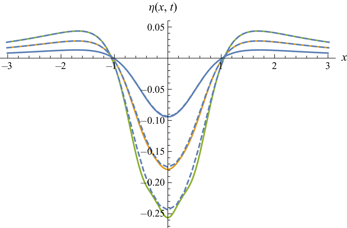
Figure 2. Symmetric dipole-type downward pressure impulse ($A=1, B=0$). Surface shape at $t=0.1$, 0.2, 0.3. Second-order Lagrangian solution (dashed) versus third-order Eulerian solution (solid lines).

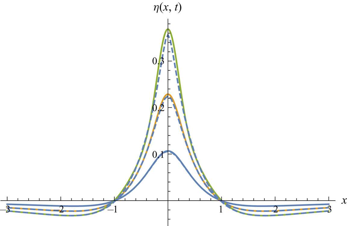
Figure 3. Symmetric dipole-type upward pressure impulse ($A=-1, B=0$). Surface shape at $t=0.1$, 0.2, 0.3. Second-order Lagrangian solution (dashed) versus third-order Eulerian solution (solid lines).

Figure 4. Antisymmetric dipole-type pressure impulse ($A=0, B=1$). Surface shape at $t=0.1$, 0.2, 0.3. Second-order Lagrangian solution (dashed) versus third-order Eulerian solution (solid lines).

Figure 5. Asymmetric dipole-type pressure impulse, downward in centre ($A=1, B=1$). Surface shape at $t=0.1$, 0.2, 0.3. Second-order Lagrangian solution (dashed) versus third-order Eulerian solution (solid lines).

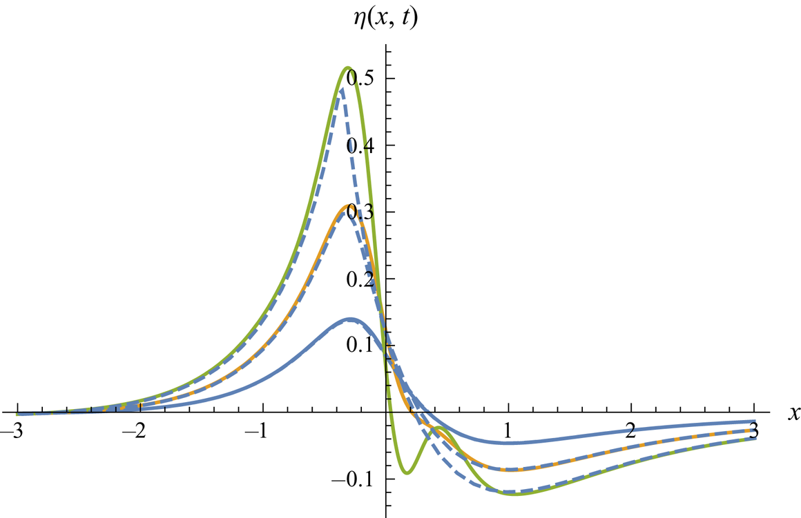
Figure 6. Asymmetric dipole-type pressure impulse, upward in centre ($A=-1, B=1$). Surface shape at $t=0.1$, 0.2, 0.3. Second-order Lagrangian solution (dashed) versus third-order Eulerian solution (solid lines).

The nonlinear effects are important in all these cases, which is demonstrated by comparing figures 2 and 3. The only difference between these two cases is the sign of the symmetric pressure impulse, which means that the solution for $A=-1, B=0$ would simply be a mirror image of the solution for $A=1, B=0$, according to linear theory. Linear theory without gravity would give linear growth of the surface profile. The case of downward pressure impulse ($A=1$) is shown in figure 2, while the mirror image of an upward impulsive suction ($A=-1$) is shown in figure 3. The latter case gives a more narrow and tall surface peak, compared with the broader and less deep trough in figure 2. This visible difference is due to the opposite direction of the forced tangential motions of surface particles.

Figure 4 shows three surface snapshots for an antisymmetric pressure impulse $A=0, B=1$, where we note the developing deviation from an antisymmetric surface shape, which is due to nonlinearity. Figures 5 and 6 show two asymmetric pressure impulses, the first one with a central downward pressure impulse, the second one with a central upward suction.

We noted that the Eulerian solutions fail to converge as soon as they develop false small-scale undulations, while the Lagrangian solutions develop visible mass defects. Chen, Hsu & Hwung (Reference Chen, Hsu and Hwung2009) exposed a similar dilemma for analytical calculations of the highest standing deep-water wave. Their figure 3 revealed mass defects in their own Lagrangian calculations of surface profiles, in comparison with the Eulerian analysis by Penney & Price (Reference Penney and Price1952). This classical work obeys exact mass balance, but suffers from false undulations of truncated Fourier series. These two theories do not fully cope with the excellent experiments by Taylor (Reference Taylor1953), but it should be mentioned that Grant (Reference Grant1973) overcame these difficulties by a conformal mapping technique leading to an accurate prediction of the highest standing deep-water wave.

Only numerical simulations of the full nonlinear process will handle the similar challenges for our present problem, and will be carried out for quadrupole-type pressure impulses. We do not present numerical simulations for dipole-type pressure impulses, because the spatial decay of dipole forcing is too slow for our numerical method, where we apply periodic boundary conditions.

5. Oblique quadrupole-type pressure impulse

The second example from Part 1 to third order is the following first-order quadrupole-type potential at the surface

(5.1)\begin{equation} - \phi_1(a, 0) = A f_2(a, 0) + B g_2(a, 0), \end{equation}

where $A$ and $B$ are dimensionless amplitudes for the symmetric and antisymmetric contribution to the pressure impulse. Figure 7 illustrates the different types of quadrupole-type pressure impulses, where $\vert A \vert$ and $\vert B \vert$ will be chosen as either one or zero.

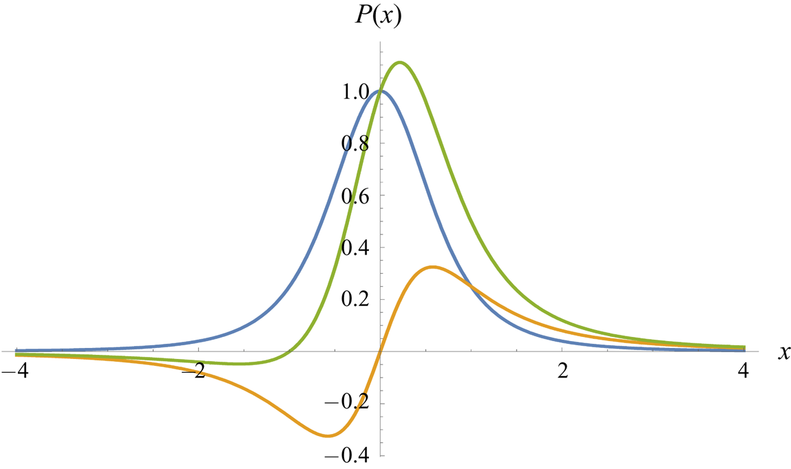
Figure 7. Quadrupole-type distributions of pressure impulses $P(x)$. The downward symmetric case $A=1, B=0$. The asymmetric case $A=0, B=1$. An antisymmetric case $A=B=1$.

Since this symmetric case (with $A=1, B=0$) was studied numerically in Part 1, we recall some findings. The free surface could easily break after the emergence of relatively tall and narrow surface peaks, where the flow became essentially nonlinear during a rapid upward motion, while the remaining oscillatory flow did not depart very much from linear theory. The strongest downward pressure-impulse amplitude (expressed in gravitational variables) that we were able to compute numerically, was $P_0 = 0.5$, which is equivalent to the dimensionless gravity parameter $G=4$. This value exceeds the upper limit of $G$ for strong nonlinearities to be able to evolve before the gravitational dispersion reduces nonlinearity. With an upward impulsive suction, the free surface is even more vulnerable for breaking, so that non-breaking flow may only develop weak nonlinearities during the first gravitational time unit. The highest absolute value that we found for impulsive suction without surface breaking was $\vert P_0 \vert = 0.225$, corresponding to the dimensionless gravity parameter $\vert G \vert = 19.75$, which is sufficiently great to suppress all third-order nonlinear effects.

The quadrupole-type pressure impulse (5.1) induces the first-order deformation

(5.2)\begin{equation} (x_1, z_1) = \boldsymbol{\nabla}_L \phi_1(a, c) = \boldsymbol{\nabla}_L (A f_2(a, c) + B g_2(a, c)), \end{equation}

where the formulas for these functions are given by Part 1 (appendix B). These deformation components generate the source term $q(a, c)$ given by (3.23)

(5.3)\begin{equation} q(a, c) = - \mbox{sign}(c) \frac{A^2 (a^2 + (4 + \vert c \vert)^2)+ 6 a A B + 9 B^2}{(a^2 + (1 + \vert c \vert)^2)^4}. \end{equation}

This source term $q(a, c)$ is to be inserted in the Green's function integral for 2-D Poisson equation (3.24). Again we evaluate the free-surface deformation by an approximation (4.8). In the numerical evaluations of the integral (4.7) for the quadrupole-type of pressure impulses, we choose the value $L=5$.

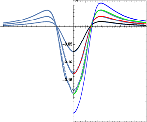
Figures 8–12 show surface snapshots for dimensionless times $t=0.05$, 0.1, 0.15 for five basic cases of quadrupole-type pressure impulses, for the non-gravitational nonlinear free-surface flow generated by a strong pressure impulse. The dashed curves represent our Lagrangian solutions, while solid lines represent the third-order Eulerian solutions from Part 1. These solutions agree very well up to $t=0.1$, but for $t=0.15$ there are serious discrepancies. Again false oscillations evolve in the Eulerian solution, while the Lagrangian solution exposes a visible mass defect. These flows from quadrupole-type forcing compare with the slower spatial decay of similar dipole-type forcing in figures 2–6.

Figure 8. Symmetric quadrupole-type downward pressure impulse ($A=1, B=0$). Surface shape at $t=0.05$, 0.1, 0.15. Second-order Lagrangian solution (dashed) versus third-order Eulerian solution (solid lines).

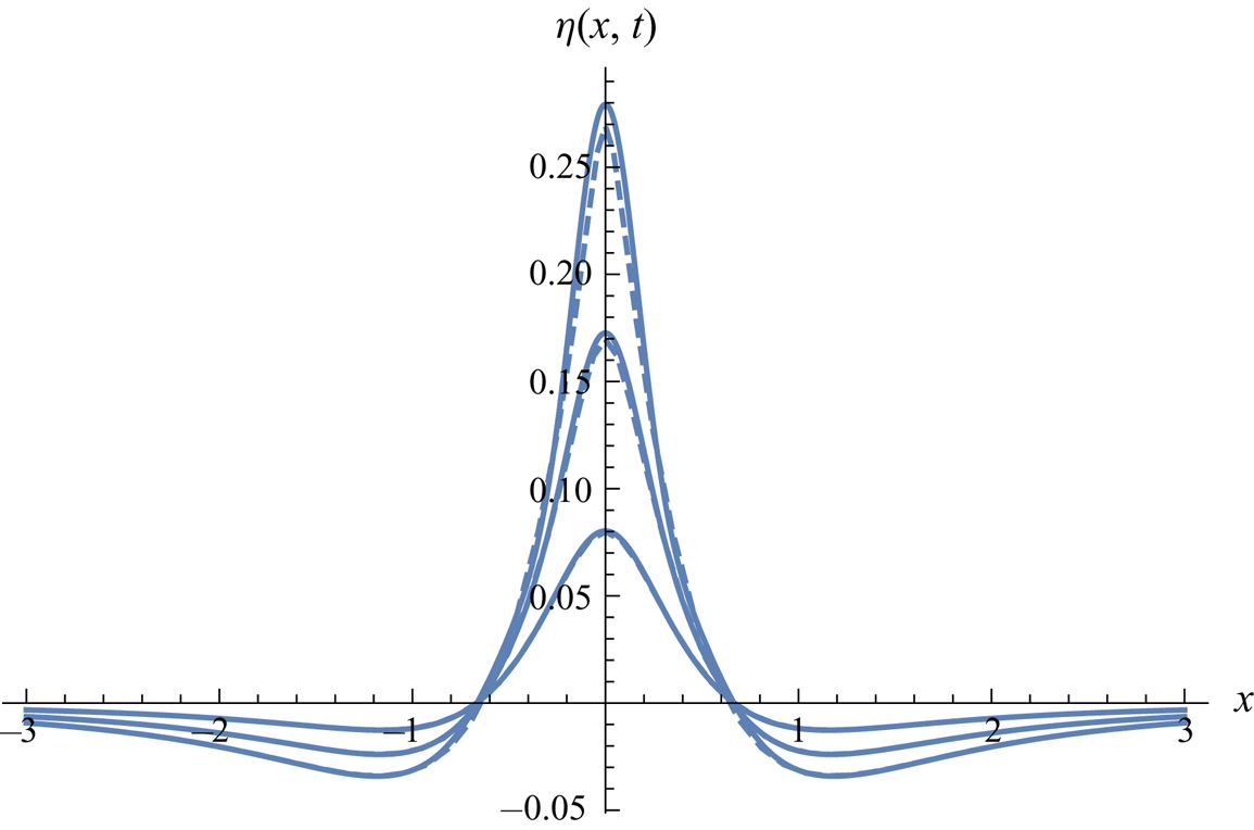
Figure 9. Symmetric quadrupole-type upward pressure impulse ($A=-1, B=0$). Surface shape at $t=0.05$, 0.1, 0.15. Second-order Lagrangian solution (dashed) versus third-order Eulerian solution (solid lines).

Figure 10. Antisymmetric quadrupole-type pressure impulse ($A=0, B=1$). Surface shape at $t=0.05$, 0.1, 0.15. Second-order Lagrangian solution (dashed) versus third-order Eulerian solution (solid lines).

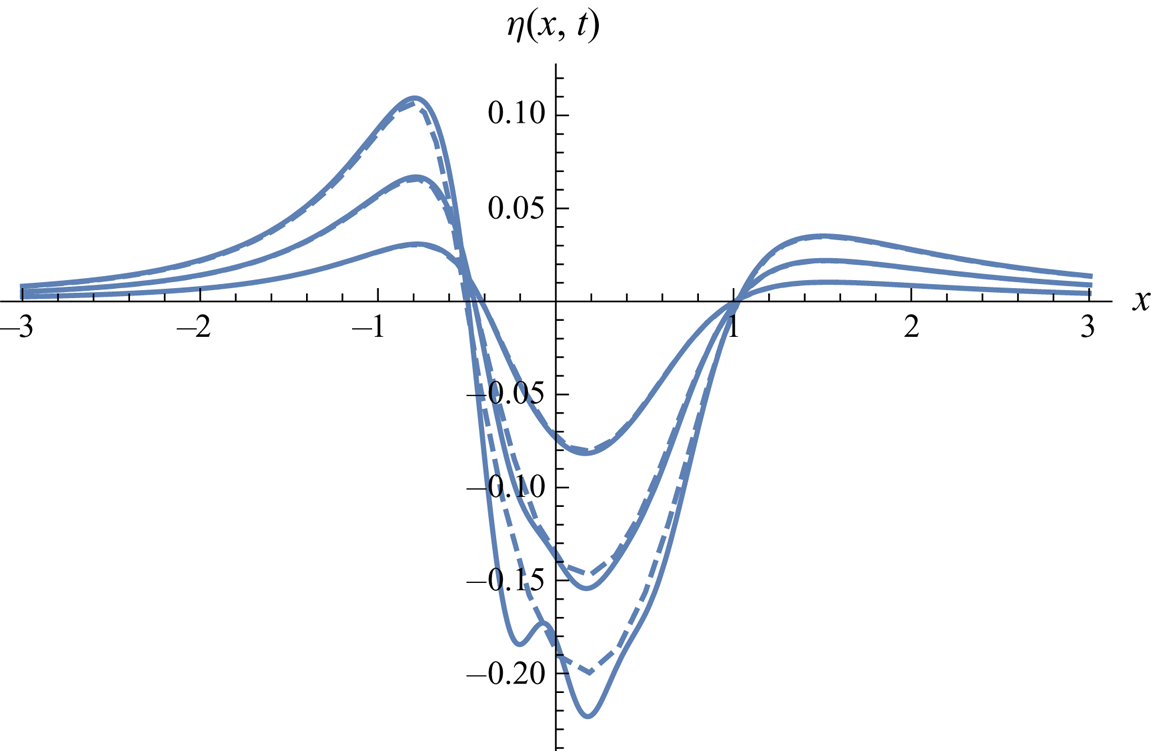
Figure 11. Asymmetric quadrupole-type pressure impulse, downward in centre ($A=1, B=1$). Surface shape at $t=0.05$, 0.1, 0.15. Second-order Lagrangian solution (dashed) versus third-order Eulerian solution (solid lines).

Figure 12. Asymmetric quadrupole-type pressure impulse, upward in centre ($A=-1, B=1$). Surface shape at $t=0.05$, 0.1, 0.15. Second-order Lagrangian solution (dashed) versus third-order Eulerian solution (solid lines).

6. Simulations for quadrupole-type pressure impulse

We will now compare these analytical results for the early nonlinear flow with our numerical method described in Part 1 (appendix C). The comparison will be limited to non-gravitational flows, because our analytical theories cannot capture gravitational oscillations. Only the first gravitational bounce back enters our third-order Eulerian small-time expansion, so we have to rely on the numerical simulations as far as the oscillatory gravitational flow is concerned.

In the numerical simulations of fully developed wave motion in Part 1, we found that moderately steep surface peaks will give divergence in the numerical methods, which is interpreted as surface breaking. This can be understood by the fact that slender surface peaks will have very little excess pressure, and in their downward motion these fluid masses will achieve almost free fall. A fluid mass with a free surface that approximately reaches free fall will induce breaking of its free surface before its downward motion is stopped.

The numerical method relies on a dimension-reduced model and is described in detail in Part 1. The spatial variable is resolved with 4096 grid points on a length of $\varGamma =20$. In the following figures, only the smaller region $[-3,3]$ is shown, represented by approximately 1230 points. The integration domain is chosen large to allow for periodic boundary conditions, which are essential for the code. The boundaries in the early times are far away from the surface elevations and have no influence. The time step is fixed with ${\rm \Delta} t = 3\times 10^{-5}$.

The code is run for $g=0$, as initial condition a flat surface with vanishing velocity is assumed. The pressure in the beginning is described by (4.3) and acts ‘infinitesimally short’, what is numerically realized by approaching the integral in (3.5) by a rectangle

(6.1)\begin{equation} P = \int_0^{0^+} p(t) \,\textrm{d}t = p(t)\delta t, \end{equation}

where $P$ being the pressure impulse and $p(t)$ the pressure

(6.2)\begin{equation} p(t) = \begin{cases} P/\delta t, & 0\le t \le \delta t, \\ 0, & \delta t < t, \end{cases}\end{equation}

with $\delta t = 20{\rm \Delta} t$.

The results are shown in figures 13–17 for the same parameters and times as in figures 8–12, where a last time interval is added, $t=0.2$. After this time, the code diverges for certain cases, which can be already noticed by the rather sharp profiles shown in figures 14 and 17.

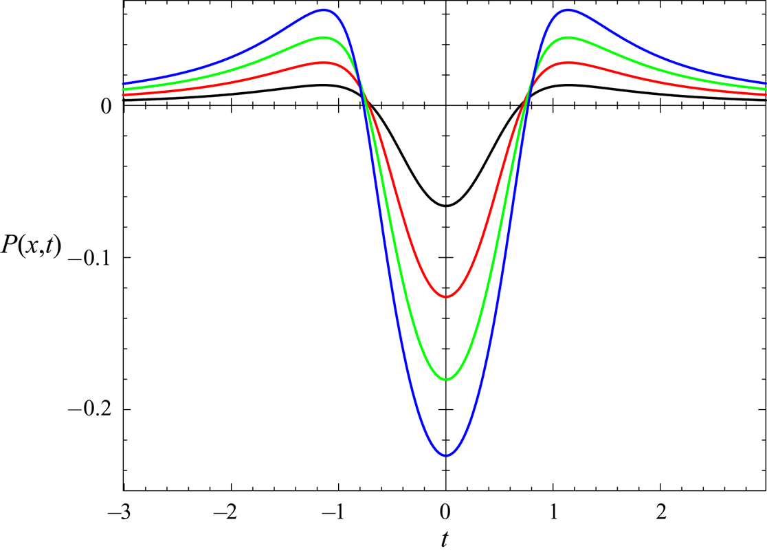
Figure 13. Numerical solution for the pressure impulse of figure 8 at $t=0.05$, 0.1, 0.15, 0.2.

Figure 14. Numerical solution for the pressure impulse of figure 9 at $t=0.05$, 0.1, 0.15, 0.2.

Figure 15. Numerical solution for the pressure impulse of figure 10 at $t=0.05$, 0.1, 0.15, 0.2.

Figure 16. Numerical solution for the pressure impulse of figure 11 at $t=0.05$, 0.1, 0.15, 0.2.

Figure 17. Numerical solution for the pressure impulse of figure 12 at $t=0.05$, 0.1, 0.15, 0.2.

7. Summary and general conclusions

The present work, presented in two parts, is concerned with the classical Cauchy–Poisson problem for initiation of water waves. The same nonlinear problem of an initiated free-surface flow is solved by two different analytical methods based on the Eulerian (Part 1) and Lagrangian description of motion (Part 2). These two analytical solutions are compared with a numerical simulation of the full nonlinear problem, representing a third solution method for the same problem.

We investigate an instantaneous pressure impulse on an initially horizontal surface. This is a second category of Cauchy–Poisson problems for water waves, where the first category is a surface elevation released from rest under gravity. The flow initiation by a pressure impulse is mathematically equivalent to specifying the initial normal velocity. The induced free-surface flow will evolve strong nonlinearities when the pressure impulse on the surface has high amplitude, measured in gravitational units. If the localized pressure impulse is weak compared with gravity, the induced deep-water wave packets will only be moderately nonlinear, with nonlinearities decreasing with time, due to the dispersive nature of deep-water waves.

Up–down asymmetry emerges in the vertical flow, since a surface crest tends to be narrow while a surface trough becomes broader, as was noted by Longuet-Higgins & Dommermuth (Reference Longuet-Higgins and Dommermuth2001). Simple arguments can be presented to explain the narrow peaks and the broader troughs that arise in the early nonlinear flow: the tangential initial velocity is outward from a trough and inward to a peak. Surface particles slide away from a surface trough to make it wider. The opposite mechanism is that surface particles pile up around a surface peak to make it more narrow. These nonlinear effects are captured more easily in a Lagrangian description, compared to an Eulerian description.

We work with two categories of pressure-impulse distributions: dipole-type distributions and quadrupole-type distributions, with five computed cases for each category. For developing the Eulerian small-time expansion in Part 1 we specified a time derivative for the surface

(7.1)\begin{equation} \left(\frac{\textrm{d}}{\textrm{d}t}\right)_{surface} = \frac{\partial}{\partial t} + \frac{\partial \eta}{\partial t} \frac{\partial}{\partial z}, \end{equation}

where the surface elevation takes only vertical motion into account, so that the horizontal motion of the surface particles does not count. The penalty for disregarding on purpose the initial tangential motion of the surface particles is the complicated second and third-order surface elevations, but the Eulerian solution is exact up to each order.

In Part 1 we also present a numerical method for the fully nonlinear free-surface flow. Calculations are performed for some quadrupole-type pressure impulses of moderate strength, where an oscillatory surface wave can develop without breaking of the free surface. It is impossible to develop a small-time expansion that accounts for a full oscillation period for the surface waves. The validity of the small-time expansion relies on the relevance of the initially delivered momentum, which is gradually absorbed by gravity so that it vanishes during the first oscillation period.

Part 2 develops a second-order small-time expansion in the Lagrangian description of motion. The Lagrangian description follows the fluid particles in their motion, in contrast to the strictly vertical surface motion of the Eulerian description. Our comparisons of all three solution methods for the fully nonlinear flow are given in Part 2. These comparisons are restricted to the non-gravitational case of inertial flow, as set by the initiation of vertical momentum from the pressure impulse. Before the Eulerian and Lagrangian small-time expansions break down, they show good agreement with one another. These two descriptions are complementary in several ways. The strength of the Eulerian method is that it is exact to the third order in the small-time expansion, with a finite number of terms. The Lagrangian method is more versatile and gives a good second-order solution, but it requires a numerical approximation of its solution integral, which forbids an extension of the analytical Lagrangian solution to third or higher order in the small-time expansion. A disadvantage with our Eulerian method is that it is highly specialized and works only for two special classes of pressure impulses, either of the dipole type or the quadrupole type.

The agreement between the Eulerian and Lagrangian solutions for the surface elevations generated pressure impulses is good until the Eulerian solution develops non-physical undulations, while the Lagrangian solution reveals a visible mass defect. A second-order Lagrangian solution may compete in accuracy with a third-order Eulerian solution because it takes the initial horizontal velocity directly into account, already in the leading order.

In a semi-infinite fluid domain with no solid boundaries present, it is known that a way of causing strongly nonlinear deep-water waves is to apply an excess surface pressure during a time interval. We therefore choose to initiate a normal velocity at the surface by a pressure impulse, and the subsequent free-surface flow may evolve strong nonlinearities. From dimensional analysis we expect that the threshold of surface breaking corresponds to a dimensionless pressure-impulse amplitude $P_0/(\rho \sqrt {g L^3})$ of order unity. This estimate is in reasonable agreement with our numerical simulations, which give non-breaking waves up to a value about 0.5 for this pressure-impulse amplitude.

The present numerical method works with periodic boundary conditions, which means that the dipole distributions for the pressure impulse is inconvenient for comparison because of its slow spatial decay. We have therefore only considered the quadrupole-type distributions of pressure impulses. The full numerical solution follows both these analytical solutions closely as long as they agree mutually. The strength of the analytical results is the representation of early nonlinearities independent of gravity. As soon as gravity takes over, we have to rely on the numerical results.

The present problem gives an opportunity to follow the evolution of strong free-surface nonlinearities from initial states, by three independent mathematical methods. The strong early nonlinear process lasts as long as the kinetic energy is considerably greater than the gravitational potential energy. It is difficult to come closer to transient surface breaking by analytical methods than what we have achieved here. The type of breaking that occurs in this physical problem, is exceptional since its cause is the forced initial impulsive flow. Breaking may only occur early in the initial interval of a gravitational time unit, while the initially delivered vertical momentum is dominating. The later gravitational flow will be only moderately nonlinear, which is the usual behaviour of free gravity waves in deep water.

We started this work by referring to slamming theory, which is a mathematically challenging field of technological importance (Korobkin & Pukhnachov Reference Korobkin and Pukhnachov1988). Our advantage over slamming theory is that we have a consistent model for the early evolution of free-surface nonlinearities. However, if we want to interpret the present results in the context of slamming, there are several shortcomings. (i) The relationship between initial forcing and induced surface motion is troublesome, if we want to interpret the forcing as the impact of a solid body. (ii) Immediately after the impact, there is no body in the fluid at all, according to our theory. (iii) We have to cover the entire surface with a non-zero pressure impulse, to avoid the free-surface singularities of slamming theory. The far-field pressure impulse must decay spatially as least at the rate of a quadrupole field in order to approach a free-surface behaviour towards infinity. We observe from our solutions that the range of our small-time expansion is smaller for the quadrupole-type pressure impulse, in comparison with the dipole impulse. Thus the range of our consistent nonlinear theory is reduced, as we get closer to a slamming model. The destiny of nonlinear slamming theory appears to be a permanent balancing between compromised physical realism and ill-posed mathematical problems.

Declaration of interests

The authors report no conflict of interest.