


1. Introduction
Turbulent boundary-layer trailing-edge (TBL-TE) noise (Brooks, Pope & Marcolini Reference Brooks, Pope and Marcolini1989) is one of the main noise generation mechanisms of various aerodynamic bodies, including wind turbine blades (Oerlemans, Sijtsma & López Reference Oerlemans, Sijtsma and López2007; Oerlemans et al. Reference Oerlemans, Fisher, Maeder and Kögler2009) and high-lift devices on aircraft (Revell et al. Reference Revell1997; Howe Reference Howe1982). It is produced by the scattering of unsteady pressure fluctuations underneath a turbulent boundary layer when a geometrical singularity, such as a TE (Howe Reference Howe1978), is present. Nevertheless, as noise regulations in both the aviation and wind turbine industries are becoming more strict, it is of great interest in the aeroacoustic communities to obtain effective approaches for attenuating TBL-TE noise. Some examples of passive noise mitigation techniques include TE serrations (Oerlemans et al. Reference Oerlemans, Fisher, Maeder and Kögler2009; Gruber, Joseph & Chong Reference Gruber, Joseph and Chong2010; Jones & Sandberg Reference Jones and Sandberg2012; Chong et al. Reference Chong, Vathylakis, Joseph and Gruber2013; León et al. Reference León, Merino-Martínez, Ragni, Avallone and Snellen2016; Avallone et al. Reference Avallone, van der Velden, Ragni and Casalino2018) and permeable (porous) TE (Hayden Reference Hayden1973; Geyer & Sarradj Reference Geyer and Sarradj2014; Herr et al. Reference Herr, Rossignol, Delfs, Lippitz and Mössner2014; Vathylakis, Chong & Joseph Reference Vathylakis, Chong and Joseph2015; Rubio Carpio et al. Reference Rubio Carpio, Merino Martinez, Avallone, Ragni, Snellen and van der Zwaag2017; Ananthan et al. Reference Ananthan, Bernicke, Akkermans, Hu and Liu2020). Unlike serrations, which are often manufactured as TE add-ons (or TE extensions), porous materials are usually employed as inserts that replace the aft section of aerofoils.
One of the earliest implementations of porosity for aerodynamic noise attenuation was reported by Hayden (Reference Hayden1973). They investigated a case of jet–flap interaction noise, in which applying a porous flap edge was found to reduce noise by more than 10 dB. Many other studies were aimed at determining the role of different porous material parameters, such as permeability, porosity and form coefficient (Ingham & Pop Reference Ingham and Pop1998), in affecting the noise reduction level. Porous TE inserts with higher permeability have been found to produce better noise reduction in general (Geyer, Sarradj & Fritzsche Reference Geyer, Sarradj and Fritzsche2010; Herr et al. Reference Herr, Rossignol, Delfs, Lippitz and Mössner2014; Rubio Carpio et al. Reference Rubio Carpio, Merino Martinez, Avallone, Ragni, Snellen and van der Zwaag2017). However, a fully porous aerofoil was considered to be undesirable as it results in substantial aerodynamic penalty (Sarradj & Geyer Reference Sarradj and Geyer2007). Although Geyer & Sarradj (Reference Geyer and Sarradj2014) found that a longer porous TE extent would improve noise reduction, they suggested to limit the extent of the porosity treatment at the aft section of the aerofoil as an acceptable trade-off against aerodynamic performance degradation.
Noise generation at a porous surface has also been examined analytically. The problem of turbulence scattering on a perforated plate has been presented in Williams (Reference Williams1972), who determined that, in the limit of low frequencies, a perforated plate with high porosity would produce predominantly dipole-type sources whereas monopoles would become more relevant for the low-porosity case. Howe (Reference Howe1979) studied the noise generation by a flat plate with a porous edge extension and found that the porous edge emitted lower sound amplitude, but noise was scattered at locations where surface impedance discontinuity is found, e.g. at the location where the solid segment ends and the porous extension begins, as well as at the downstream edge of the porous extension. This finding was later confirmed in many other investigations (Delfs et al. Reference Delfs, Faßmann, Lippitz, Lummer, Mößner, Müller, Rurkowska and Uphoff2014; Kisil & Ayton Reference Kisil and Ayton2018; Rubio Carpio et al. Reference Rubio Carpio, Avallone, Ragni, Snellen and van der Zwaag2019a). Additionally, it can be argued that Howe was also the first to suggest that implementing chordwise-varying porosity would further improve the noise attenuation level. More recently, Jaworski & Peake (Reference Jaworski and Peake2013) employed the Wiener–Hopf technique to obtain an analytical prediction on a semi-infinite poroelastic plate, where it was found that the acoustic power scattered by a porous plate scales with the sixth power of the Mach number, which implies less efficient scattering compared to that of a solid edge (Williams & Hall Reference Williams and Hall1970). Moreover, they predicted that the noise reduction of the porous plate would be mainly found in the low frequency region. Cavalieri, Wolf & Jaworski (Reference Cavalieri, Wolf and Jaworski2016) later extended this investigation to include the effect of a finite chord length, and the porous plate was found to alter the noise directivity into a dipole-like shape, unlike for the solid one, which exhibits cardioid-like directivity.
Other investigations were carried out to determine the noise mitigation mechanisms of a porous TE. Herr et al. (Reference Herr, Rossignol, Delfs, Lippitz and Mössner2014) and Delfs et al. (Reference Delfs, Faßmann, Lippitz, Lummer, Mößner, Müller, Rurkowska and Uphoff2014) suggested that the interaction between pressure fluctuations at the pressure and suction sides of the porous TE, referred to as the pressure release process, is responsible for promoting noise attenuation. They arrived at this conclusion after observing that there was no noise reduction when one side of the porous insert was covered with non-permeable tape. More recently, Rubio Carpio, Avallone & Ragni (Reference Rubio Carpio, Avallone and Ragni2018) took a different approach by applying a layer of adhesive at the symmetry plane of a metal-foam insert, which was subsequently referred to as a non-permeable porous insert. This approach was taken to preserve the surface roughness of the porous insert. The non-permeable insert was no longer reducing noise at low frequencies, but the high-frequency excess noise remained, confirming that the latter can be associated with the surface roughness effect. In Rubio Carpio et al. (Reference Rubio Carpio, Avallone, Ragni, Snellen and van der Zwaag2019a), they also observed that turbulent fluctuations in the boundary layers on both sides of the porous TE remained correlated when the adhesive layer was absent, confirming the pressure release process.
To obtain information on flow field details inside and surrounding a porous TE, high-fidelity numerical simulations offer more flexibility, although such simulations can be quite costly when involving porous materials with relatively small pore dimension compared to the overall length scale of the body (Freed Reference Freed1998). As a workaround, the macroscopic effects of the porous TE on the flow field are taken into account using porous medium models. Recently, Ananthan et al. (Reference Ananthan, Bernicke, Akkermans, Hu and Liu2020) applied a porous medium model in a numerical investigation on a DLR F16 aerofoil. The porous insert was modelled as an equivalent fluid region using volume-averaged Navier–Stokes equations where additional flow resistance terms, based on Darcy's law, were added (Ingham & Pop Reference Ingham and Pop1998). The authors were able to observe the role of the porous medium in decreasing the spanwise coherence of surface pressure fluctuations while also reducing the convection velocity, both of which were linked to noise attenuation. Using an analogous approach, Teruna et al. (Reference Teruna, Manegar, Avallone, Ragni, Casalino and Carolus2020) employed a porous medium model in a lattice Boltzmann (LB) solver to replicate the experiments of Rubio Carpio et al. (Reference Rubio Carpio, Avallone, Ragni, Snellen and van der Zwaag2019a). The authors confirmed that when the blocked porous TE was used, no noise reduction could be observed. They also proposed two noise mitigation mechanisms of the metal-foam insert: (1) reduced scattering efficiency at the actual TE due to the milder impedance jump; and (2) destructive interference between sound sources that are distributed along the porous medium surface.
Nevertheless, the use of porous medium models introduces another layer of uncertainty into the investigation, and it remains an open question whether the noise reduction mechanisms discussed in Teruna et al. (Reference Teruna, Manegar, Avallone, Ragni, Casalino and Carolus2020) are still appropriate when permeability is realised using a porous geometry instead of an equivalent fluid region. For this purpose, a synthetic unit-cell geometry has been designed and utilised to construct a porous TE insert, which is later manufactured and tested in experiments, allowing for direct comparison with simulation results. This study also looks further into how the pressure release process, which is realised by permeability, alters the noise source characteristics at the TE. Additionally, a partially blocked porous insert has been considered to elucidate the role of different segments of the porous TE in noise attenuation. Furthermore, this allows a link between the permeable extent of the porous TE and the noise attenuation level to be established.
The rest of this paper is organised as follows. The numerical procedure is briefly reported in § 2. A description of the simulation set-up is presented in § 3. Validation and verification of the simulation results will be shown in § 4, followed by in-depth analyses of the far-field noise results in § 5. Afterwards, the effects of the porous insert on the flow field are discussed in § 6. Then § 7 briefly discusses the link between the present observations with the authors’ past work. The paper is concluded in § 8, where an outlook is also provided.
2. Methodology
2.1. Flow solver
The present work employs a commercial LB solver, SIMULIA PowerFLOW 5.4b, to solve the flow field in the simulation domain. This solver has been previously used for TBL-TE noise investigations (Moreau et al. Reference Moreau, Sanjosé, Perot and Kim2011; Sanjosé et al. Reference Sanjosé, Méon, Moreau, Idier and Laffay2014; Avallone et al. Reference Avallone, van der Velden, Ragni and Casalino2018). The LB method describes fluid phenomena at mesoscopic scale in a statistical sense. It solves the discrete Boltzmann equation for particle distribution functions in a predefined number of velocity directions. In the LB method, fluid phenomena are governed by two processes, namely advection and collision, which are mathematically described as follows:
 \begin{equation} \frac{\partial{\boldsymbol{F}}}{\partial{t}} + \boldsymbol{V}\boldsymbol{\cdot} \boldsymbol{\nabla} \boldsymbol{F} = \boldsymbol{\mathcal{C}}, \end{equation}
where  $\boldsymbol {F}(\boldsymbol {x},t)$ is the particle distribution function in space ( $\boldsymbol {x}$) and time ( $t$),
$t$),  $\boldsymbol {V}$ is the particle velocity and $\boldsymbol {\mathcal {C}}$ is the collision operator. The employed implementation of the discrete LB equation uses 19 velocity directions in three dimensions (i.e. D3Q19) with a third-order truncation of the Chapman–Enskog expansion, which has been shown to accurately approximate the Navier–Stokes equations for perfect gas flow at low Mach number and isothermal conditions (Chen, Chen & Matthaeus Reference Chen, Chen and Matthaeus1992). The discretised form of the LB is written as
 \begin{equation} \boldsymbol{F}_{n}(\boldsymbol{x} + \boldsymbol{V}_{n} {\rm \Delta} t,t+{\rm \Delta} t) - \boldsymbol{F}_{n}(\boldsymbol{x} , t) = \boldsymbol{\mathcal{C}}_{n} (\boldsymbol{x},t), \end{equation}
and it is solved on a Cartesian grid that is referred to as a lattice. In (2.2),  $\boldsymbol {F}_{n}$ is the particle distribution function along the $n$th direction with respect to the lattice orientation and $\boldsymbol {V}_{n}$ is the discrete particle velocity vector. The collision term $\boldsymbol {\mathcal {C}}_{n}$ is represented using the Bhatnagar–Gross–Krook model (Bhatnagar, Gross & Krook Reference Bhatnagar, Gross and Krook1954):
 \begin{equation} \boldsymbol{\mathcal{C}}_{n} ={-} \frac{{\rm \Delta} t}{\tau} [ \boldsymbol{F}_{n}(\boldsymbol{x},t) - \boldsymbol{F}_{n}^{{eq}}(\boldsymbol{x},t) ]. \end{equation}
Here  $\tau$ is the relaxation time, which is a function of fluid viscosity and temperature; and $\boldsymbol {F}_{n}^{{eq}}$ is the equilibrium Maxwell–Boltzmann distribution function, which is approximated by a second-order expansion (Chen et al. Reference Chen, Chen and Matthaeus1992) as
 \begin{equation} \boldsymbol{F}_{n}^{{eq}}=\rho\boldsymbol{\omega}_{n} \left [ 1+\frac{\boldsymbol{V}_{n}\boldsymbol{u}}{a^{2}_s}+\frac{(\boldsymbol{V}_{n}\boldsymbol{u})^{2}}{2a^{4}_s} -\frac{\lvert \boldsymbol{u} \rvert ^{2}}{2a^{2}_s} \right ], \end{equation}
where  $\boldsymbol {\omega }_{n}$ are fixed weight functions based on the D3Q19 model (Chen et al. Reference Chen, Chen and Matthaeus1992) and $a_s = {1}/{\sqrt {3}}$ is the non-dimensional speed of sound in lattice units. After solving (2.2) to obtain the distribution functions, macroscopic flow variables, such as density $\rho$ and velocity $\boldsymbol {u}$, are computed by taking the appropriate moment of the distribution function as follows:
 \begin{gather} \rho(\boldsymbol{x},t) = \sum_{{n}} F_{n}(\boldsymbol{x},t), \end{gather}
 \begin{gather}\rho\boldsymbol{u}(\boldsymbol{x},t) = \sum_{{n}} \boldsymbol{V}_{{n}} F_{n}(\boldsymbol{x},t). \end{gather}
 Turbulence in the flow is resolved using a very large eddy simulation (VLES) approach. In this implementation, an eddy viscosity model is introduced into the collision term of the LB equation (Teixeira Reference Teixeira1998). The solver employs a modified  $k$–
$k$– $\epsilon$ two-equation model based on the renormalisation group (RNG) formulation, which is used to compute an effective relaxation time $\tau _{{eff}}$ as follows:
 \begin{equation} \tau_{{eff}}=\tau+C_\mu \frac{k^{2}/\epsilon}{\sqrt{1+\eta^{2}}}. \end{equation}
Here  $C_\mu = 0.09$ and $\eta$ are a combination of the local strain $k \lvert \boldsymbol {S}/\epsilon \rvert$, local vorticity $k \lvert \boldsymbol {\omega }/\epsilon \rvert$ and local helicity parameters. The effective relaxation time $\tau _{{eff}}$ replaces the original relaxation time in (2.2), which in turn calibrates the LB solver to the characteristic time scales of the turbulence in the flow field. Hence, the two-equation turbulence model effectively modifies the relaxation properties of the system, which enables the development of large turbulent eddies in the simulation domain. Moreover, it can be shown using the Chapman–Enskog expansion that the nonlinearity of Reynolds stresses is captured (Teixeira Reference Teixeira1998; Chen et al. Reference Chen, Orszag, Staroselsky and Succi2004). Hence the present application of the $k$–
$k$– $\epsilon$ model is different from that in Reynolds-averaged Navier–Stokes, where, in the latter, quantities derived from the turbulence model are not used to define Reynolds stresses explicitly.
The simulation domain is discretised into cubic volume elements referred to as ‘voxels’ (i.e. volumetric pixels). Refinement regions are applied to the simulation domain based on the desired spatial resolution such that the voxel size between two adjacent regions varies by a factor of 2. Solid bodies are facetised using ‘surfels’ (i.e. surface pixels) at locations where they intersect with voxels. The process of generating voxels and surfels is fully automated, allowing for complex geometrical details, such as that of the porous material, to be discretised with relative ease. The boundary condition at a solid wall is realised by applying appropriate particle interactions in the collision term of the LB scheme, such as a particle bounce-back process for a no-slip wall and specular reflection for a slip wall, respectively (Chen, Teixeira & Molvig Reference Chen, Teixeira and Molvig1998). A wall model is applied at the first wall-adjacent grid (Teixeira Reference Teixeira1998; Wilcox Reference Wilcox1998). It is based on the generalised law-of-the-wall model (Launder & Spalding Reference Launder and Spalding1983), which has been extended to consider the effects of pressure gradient.
2.2. Far-field noise computations
The solution of the LB scheme is suitable for resolving acoustic perturbations in the simulation domain since it is inherently compressible and unsteady, combined with low dissipation and dispersion characteristics. For far-field noise prediction, however, direct acoustic computation is often impracticable, especially as a minimum of approximately 15 voxels is required to resolve the acoustic wavelength corresponding to the frequency of interest (Casalino, Hazir & Mann Reference Casalino, Hazir and Mann2018). Instead, employing an acoustic analogy is more often the feasible approach. In the present study, far-field noise is computed using the Ffowcs Williams & Hawkings (Reference Ffowcs Williams and Hawkings1969) (FW-H) analogy based on the formulation 1A of Farassat & Succi (Reference Farassat and Succi1980) extended to a convective wave equation (Brès, Pérot & Freed Reference Brès, Pérot and Freed2009). The formulation has been implemented in the time domain with an advanced-time approach (Casalino Reference Casalino2003). The integration surface can be determined to be on a solid surface or on a permeable one, and the formulation of the acoustic analogy is adjusted accordingly. The input for the acoustic analogy is recorded at the finest voxel resolution level (cutoff frequency  $\approx 250\ \textrm {kHz}$) on the aerofoil surface and at the third finest resolution level (cutoff frequency $\approx 31\ \textrm {kHz}$, or $St_c \approx 310$, where $c$ is the aerofoil chord length) on a permeable surface enclosing the aerofoil. The former approach supposes a distribution of acoustic dipoles on the aerofoil surface (Curle Reference Curle1955), while, for the latter, the contribution of the volumetric source terms (i.e. quadrupoles) is also included. The permeable surface is extended by twice the aerofoil chord length downstream of the trailing edge to capture the contribution of the aerofoil wake, but its downstream face is removed to exclude the contribution of pseudo-noise (i.e. non-radiating flow perturbations) (Casper et al. Reference Casper, Lockard, Khorrami and Streett2004; Lockard & Casper Reference Lockard and Casper2005).
3. Simulation set-up
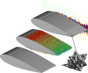
The present study employs a similar simulation set-up to that used previously by the authors (Teruna et al. Reference Teruna, Manegar, Avallone, Ragni, Casalino and Carolus2020), which is based on the experiment of Rubio Carpio et al. (Reference Rubio Carpio, Avallone and Ragni2018). A NACA 0018 aerofoil is set at zero angle of attack and it has a chord of  $c=200$ mm. Three TE configurations are investigated, as shown in figure 1: the baseline model with solid TE ( $a$), and two others equipped with permeable inserts ( $b$) and ( $c$) that replace the solid material in the last 20 % of the aerofoil chord, referred to as porous and blocked TE, respectively. The blocked TE has a thin solid partition installed along the aerofoil chord line, in between 20 % and 80 % of the porous TE extent (i.e. the last 16 % to 4 % of the aerofoil chord). Hence, this is a different treatment compared to the full-length partition previously employed in Teruna et al. (Reference Teruna, Manegar, Avallone, Ragni, Casalino and Carolus2020), but the purpose of the solid partition remains the same: it prevents the boundary layers on both sides of the TE from interacting with each other across the porous medium. The chordwise extent of the solid partition in the blocked TE has been chosen to assess the role of the pressure release process near the solid–porous junction and the actual TE.

Figure 1. A drawing of the NACA 0018 with solid ( $a$), porous ( $b$) and blocked ( $c$) TE configurations. A lateral view of the aerofoil with blocked TE is shown at bottom left, besides which is an inset depicting the unit-cell geometry.
The porous material used in the present study has a unit-cell geometry that is based on the diamond lattice structure. The unit cell consists of a network of cylindrical struts whose dimensions are reported in table 1. The unit-cell dimension is scaled to  ${D=6.36}$ mm, such that the resulting porous insert produces comparable noise reduction level and spectral features as those of the metal-foam insert previously tested in Rubio Carpio et al. (Reference Rubio Carpio, Avallone and Ragni2018) and Teruna et al. (Reference Teruna, Manegar, Avallone, Ragni, Casalino and Carolus2020). Note that the unit-cell size is different from the mean pore diameter, the latter of which is $d_p=1.2$ mm. The aerofoil span for the solid TE case equals one-fifth of that in the experiment (Teruna et al. Reference Teruna, Manegar, Avallone, Ragni, Casalino and Carolus2020), i.e. $b=0.4c=8$ cm. However, the spanwise extent of the aerofoils with the permeable TE are slightly reduced to $76.32\ \textrm {mm} = 12D$ to ensure spanwise periodicity of the unit cell. To obtain a fair comparison with the simulation results, the geometry of the porous insert is manufactured using 3-D printing for the experiment. The surface outline of the porous insert follows the solid one. This implies that some unit cells that are located near the surface are partially cut, and the resulting surface pore diameter varies between 0.45 mm and 5.3 mm. The unit-cell arrangement is also not completely symmetrical along the aerofoil chord line due to manufacturing constraints; it will be shown that this does not significantly affect the overall aerodynamic and acoustic characteristics of the porous TE.
Table 1. The geometrical properties of the diamond lattice unit cell.
The characterisation of the porous material has been carried out using a permeability test rig (Rubio Carpio et al. Reference Rubio Carpio, Merino Martinez, Avallone, Ragni, Snellen and van der Zwaag2017). Both mean pore size  $d_p$ and porosity $\phi$ can be measured from the unit-cell geometry. Differently, the permeability $K$ and form coefficient $C$ are calculated by performing a curve fit of the experimental pressure-drop test data with the Hazen–Dupuit–Darcy equation (Rubio Carpio et al. Reference Rubio Carpio, Merino Martinez, Avallone, Ragni, Snellen and van der Zwaag2017; Teruna et al. Reference Teruna, Manegar, Avallone, Casalino, Ragni, Rubio Carpio and Carolus2019). It is found in the experiment that both the permeability and form coefficient of the porous material converge once the sample is more than seven unit cells thick (i.e. the critical thickness (Dukhan & Minjeur Reference Dukhan and Minjeur2010)). These values are reported in table 2.
Table 2. The transport characteristics of the porous material.
A sketch of the computational domain is shown in figure 2. The origin of the coordinate system is defined at the midspan of the trailing edge, with the  $x$ axis aligned with the aerofoil chord, the $z$ axis with the aerofoil span and the $y$ axis perpendicular to both the $x$ and $z$ axes. Note that $x$ and $y$ can also be designated as wall-parallel and wall-normal directions when indicated as such. Hence, the aerofoil leading edge is located at $x/c=-1$, and the trailing edge at $x/c=0$. The $x$,
$x$,  $y$ and $z$ axes will be referred to as streamwise, vertical and spanwise directions, respectively. The computational domain is a rectangular box that is $100c$ long in both $x$ and $y$ directions, while its length in the $z$ direction equals $b$. To prevent acoustic field contamination due to reflection from the domain boundaries, an acoustic sponge region is applied starting from a radius of $36c$ from the origin. Static pressure $p_\infty =101\,325$ Pa and free-stream velocity $U_\infty =20$ m s $^{-1}$ are specified at the upstream, downstream, top and bottom boundaries. These flow parameters correspond to a chord-based Reynolds number of $Re_c = 2.7 \times 10^{5}$ and a free-stream Mach number of $M_\infty = {0.06}$. The lateral boundaries are defined with periodic boundary conditions. The entire aerofoil surface, including the porous medium, is specified as no-slip walls. Laminar–turbulent transition on the aerofoil is enforced using zig-zag trips (Elsinga & Westerweel Reference Elsinga and Westerweel2012) installed at $x/c=-0.8$ (i.e. 20 % of the chord length). The zig-zag trip height is $t_{trip} = 0.003c = 0.6$ mm, while the amplitude is $c_{trip} = 0.015c = 3$ mm and the wavelength is $\lambda _{trip} = 0.015c = 3$ mm. The tripping elements are the same as those in the authors’ previous study (Teruna et al. Reference Teruna, Manegar, Avallone, Ragni, Casalino and Carolus2020).

Figure 2. A sketch of the computational domain. Note that dimensions are not to scale.
The simulation domain is subdivided into 10 grid refinement regions with a resolution factor of 2 between adjacent regions. This allows for an efficient use of computational resources while retaining sufficient spatial resolution. The finest grid resolution is specified at a region surrounding the aerofoil surface where the voxel size is equal to  $3.9\times 10^{-4}c$. As such, the height of the turbulent boundary layer near the TE ( $x/c=-0.01$) is resolved by approximately 128 voxels, and the first wall-adjacent voxel height at this location corresponds to $y^{+}=3$ for the solid TE case. This discretisation strategy produces a total of $218\times 10^{6}$ and $293 \times 10^{6}$ voxels inside the simulation domain for the solid and porous TE cases, respectively. The simulations are carried out for 20 flow passes, excluding the initial transient, on the servers of Delft University of Technology and the National Supercomputing Center (IT4Innovations) of the Czech Republic. For reference, the porous TE case requires a total of 114.400 CPU hours on a 480-core Xeon Gold 6130 platform, which is approximately three times that required for the solid TE case.
4. Grid independence study and simulation validation
In this section, the numerical solutions are assessed. The grid independence study is performed using four resolution levels that correspond to  $y^{+}$ values of the first wall-adjacent voxel height: coarse ( $y^{+}=12$), medium ( $y^{+}=6$), fine ( $y^{+}=3$) and very fine ( $y^{+}=2.1$ for solid TE and $y^{+}=1.5$ for porous TE). Note that these reference $y^{+}$ values are sampled at $x/c = -0.01$ for the solid TE case; the $y^{+}$ value for the porous TE case is slightly lower although the same grid resolution is applied in both cases. At each resolution level, grid refinement is applied uniformly across the simulation domain, identical to the procedure reported in Teruna et al. (Reference Teruna, Manegar, Avallone, Ragni, Casalino and Carolus2020). For the very fine setting, however, the porous TE case has a higher grid resolution than the solid TE one in order to maintain spanwise periodicity of the porous insert. A lateral view showing the grid arrangement surrounding the aerofoil with a porous insert is provided in figure 3.

Figure 3. A lateral view of the aerofoil with porous TE, illustrating the voxel distribution with the fine grid setting.
Figure 4 illustrates the convergence trend of the boundary-layer thickness  $\delta _{99}$ near the TE ( $x/c=-0.002$). This thickness $\delta _{99}$ is defined as the distance from the wall where the mean wall-parallel velocity is 99 % of the boundary-layer edge velocity $U_e$, which is the mean velocity in the boundary layer where the integral of the spanwise vorticity along the wall-normal direction (i.e. $\int \omega _z\,{\textrm {d} y}$) becomes asymptotic (Spalart & Watmuff Reference Spalart and Watmuff1993). Figure 4 also shows the Richardson extrapolation as empty square markers up to $y^{+} = 0.75$ using the refinement ratio $M=2$ and the order of convergence $N=3$. The convergence trend of the $\delta _{99}$ is evaluated using the grid convergence index ( ${\rm GCI}$) (Roache Reference Roache1998; Slater Reference Slater2018). The ${\rm GCI}$ allows one to estimate the deviation, as a percentage, of the numerical solution at a given grid refinement setting from that of an asymptotic solution. For the fine grid resolution ( $y^{+}=3$), the solid TE has ${GCI}_{{medium,fine}} = 0.288\,\%$ and ${GCI}_{{fine,very\,fine}} = 0.0385\,\%$; these are $0.183\,\%$ and $0.0258\,\%$, respectively, for the porous TE. Moreover, the ${\rm GCI}$ ratio is also computed as in (4.1), after which ${\rm GCI}$ ratios of 0.935 and 0.875 are obtained for solid and porous TE cases, respectively. Since the ${\rm GCI}$ values next to the fine grid resolution are relatively small, and the corresponding ${\rm GCI}$ ratios are close to unity, it can be concluded that the numerical results obtained using the fine grid resolution are already within the asymptotic range of convergence (Roache Reference Roache1998):
 \begin{equation} {GCI}_{{ratio}}\big|_{{fine},{very\,fine}} =\frac{{GCI}_{{fine,very\,fine}}}{M^{N} {GCI}_{{medium,fine}}}. \end{equation}
Figure 4. The comparison of boundary-layer thickness at  $x/c=-0.002$ for the different grid resolutions. The Richardson extrapolation of the boundary-layer thickness is plotted as empty square. The thick line at $y^{+}=3$ denotes the adopted grid resolution for the rest of the paper. Data for the solid TE case have been extracted from Teruna et al. (Reference Teruna, Manegar, Avallone, Ragni, Casalino and Carolus2020).
Additionally, the mean wall-friction coefficient ( $C_f$) is also used for evaluating grid convergence, since this quantity depends on the velocity gradient next to the wall. The $C_f$ distributions for the aforementioned grid resolution levels are illustrated in figure 5. The $C_f$ distribution for the porous TE contains interpolated data points where open pores are located. For both solid and porous TE cases, the $C_f$ variations are larger between the $y^{+}=6$ (medium) and $y^{+}=3$ (fine) simulations. This is particularly noticeable where the porous TE is located (i.e. $-0.2 < x/c <0$), since the voxels at lower resolution level are incapable of resolving the intricate details of the struts in the porous TE. However, the $C_f$ distributions are similar when comparing the fine and very fine plots. Thus, it is possible to conclude that a voxel resolution corresponding to $y^{+}=3$ is sufficient, and subsequently this resolution level is employed for the rest of this paper.

Figure 5. The comparison of mean wall-friction coefficient along the aerofoil midspan at  $-0.5 < x/c < 0$ for the different grid resolutions.
In the following, flow field and acoustic predictions from the simulation are validated against experimental results. In figure 6, the mean streamwise velocity profiles are plotted at three different locations in ( $a$), while the velocity fluctuation profiles near the TE are shown in ( $b$). It is worth mentioning that the boundary-layer profiles from the experiment have been obtained using particle image velocimetry (PIV), and, as a consequence, near-wall measurements are limited due to the presence of light reflections from the aerofoil surface (Rubio Carpio et al. Reference Rubio Carpio, Martínez, Avallone, Ragni, Snellen and van der Zwaag2019b). Nevertheless, figure 6 shows good agreement between the numerical results and the experimental ones. The differences between the flow field in the solid and porous TE cases will be discussed in detail in § 6.

Figure 6. Comparisons of flow statistics in the turbulent boundary layer. All data points have been extracted at the aerofoil midspan. Mean wall-parallel velocity ( $U$) profiles at several chordwise locations are shown in ( $a$); and profiles of root mean square (r.m.s.) of velocity fluctuations in the wall-parallel ( $u_{{rms}}$) and wall-normal ( $v_{{rms}}$) directions are shown in ( $b$). Note that ‘experiment’ is abbreviated as (exp.); and SLD is short for solid.
The power spectral density of far-field acoustic pressure  $\varPhi _n$ computed in the simulations is provided in figure 7, where the frequency is expressed in Strouhal number based on the aerofoil chord, $St_c = fc/U_\infty$. The observer location for this comparison is directly above the TE ( $x/c=0, y/c=5$). Since the aerofoil span in the simulation is smaller than in the experiment, the raw noise spectra from the simulation $\varPhi _o$ has been scaled as in (4.2) (Avallone et al. Reference Avallone, van der Velden, Ragni and Casalino2018). This scaling would also allow for direct comparison with the noise spectra from the experiment:
 \begin{equation} \varPhi_n = \varPhi_o + 10\log_{10}\left(\frac{b_{{experiment}}}{b_{{simulation}}} \right). \end{equation}
Figure 7. Comparisons of far-field noise spectra obtained using the FW-H acoustic analogy using the flow information at the aerofoil surface (surface FW-H), and at a permeable surface that encloses the aerofoil (permeable FW-H). Observer location is  $x/c=0$, $y/c=5$.
Figure 7 compares the spectra calculated using the flow field information sampled at the aerofoil surface and at a permeable surface that encloses the near-field region. The noise spectra obtained from the surface FW-H formulation are in good agreement with those from the permeable FW-H approach. This implies that the noise sources on the aerofoil are predominantly of dipole type, and thus quadrupole noise sources, such as those in the turbulent aerofoil wake, do not make a substantial contribution towards noise generation, which is typically the case for low-Mach-number flows.
The validation of the far-field acoustic spectra for both TE types is provided in figure 8. Figure 8( $a$) shows that the noise prediction from the simulation generally agrees well with the experimental measurements, except for the solid TE case at $St_c > 16$. It has been previously reported in Teruna et al. (Reference Teruna, Manegar, Avallone, Ragni, Casalino and Carolus2020) that the overestimated high-frequency noise of the solid TE originates from the zig-zag trip, whereas the experiment employs a strip of carborundum particles for triggering laminar–turbulent transition (Rubio Carpio et al. Reference Rubio Carpio, Avallone, Ragni, Snellen and van der Zwaag2019a). Such discrepancy is less apparent in the porous TE case, because the self-noise of the zig-zag trip has a lower intensity compared to the excess noise from the porous material itself. The noise reduction spectra are plotted in figure 8( $b$), where positive values refer to noise attenuation, and negative ones to noise increase. The noise reduction at low frequency reaches up to 11 dB near $St_c = 6$, with the average of 10 dB in the range $4< St_c<8$. In the mid frequency range, the noise reduction gradually decreases from $St_c=8$ and it eventually vanishes at around $St_c=16$. At higher frequencies, noise increases by around 2 dB can be found in certain frequency bands. Following this, the spectra can be divided into three frequency regions: (1) a region where large noise attenuation exists ( $4< St_c<8$); (2) a transition region where the noise attenuation level gradually decreases ( $8< St_c<16$); and (3) a region where excess noise is observed ( $16< St_c<32$). This trend is in line with past analytical studies (Jaworski & Peake Reference Jaworski and Peake2013; Cavalieri et al. Reference Cavalieri, Wolf and Jaworski2016), where the noise reduction of a perforated plate has been predicted to become smaller as frequency increases.

Figure 8. A comparison of far-field noise results between those from experiment and simulation. Panel ( $a$) shows the power spectral density of acoustic pressure ( $\varPhi _n$) and panel ( $b$) shows the difference in $\varPhi _n$ values between solid and porous TE cases.
This section has shown that the simulation results can be utilised for analysing the aeroacoustic characteristics of the porous TE inserts, which will be reported in subsequent sections. Note that, from here on, the far-field noise results presented are obtained using the surface FW-H approach.
5. Aeroacoustic characteristics of the porous trailing edge
5.1. Far-field noise intensity and directivity
The comparison of far-field noise spectra between the three cases is depicted in figure 9( $a$), and the noise reduction spectra are shown in figure 9( $b$). It is evident that the solid partition added in the blocked TE case leads to smaller noise reduction, particularly at $St_c < 6$; the noise attenuation level of the blocked TE remains similar to that of the porous TE at higher frequencies. This is in line with other experimental observations (Delfs et al. Reference Delfs, Faßmann, Lippitz, Lummer, Mößner, Müller, Rurkowska and Uphoff2014; Carpio et al. Reference Carpio, Avallone, Ragni, Snellen and van der Zwaag2020) that the noise reduction of the porous TE is directly linked to the permeable extent of the porous TE. Considering that the solid partition does not cover the full extent of the blocked TE, this suggests that altering the permeable extent of the TE mainly affects the frequency range where noise reduction can be achieved, as hinted previously in Kisil & Ayton (Reference Kisil and Ayton2018). Figure 9( $b$) also shows the presence of high-frequency excess noise ( $16 < St_c < 32$) in the blocked TE case, but the average intensity is lower than that of the porous TE case. Since the surface roughness characteristics for both types of permeable TE are identical, it is possible to consider that the permeable extent of the porous insert is also related to the excess noise production. It is worth mentioning that the diamond unit-cell geometry might be unfavourable in terms of surface roughness noise, since the unit-cell struts are oblique relative to the incoming flow direction (Clark et al. Reference Clark, Daly, Devenport, Alexander, Peake, Jaworski and Glegg2016). Moreover, the partially cut unit cells at the surface also behave as additional roughness elements (Devenport et al. Reference Devenport, Alexander, Glegg and Wang2018).

Figure 9. Panel ( $a$) compares the $\varPhi _n$ spectrum for the different TE types and panel ( $b$) shows the difference ${\rm \Delta} \varPhi _n$ relative to the solid TE. The observer location is $x/c=0, y/c=5$.
Far-field noise directivity patterns for the different TE types are illustrated in figure 10. The sound pressure spectrum  $\varPhi _n$ has been integrated in the three frequency ranges previously defined in figure 8, and these are shown in figure 10( $a$–
$a$– $c$). The frequency ranges are also expressed in terms of chord-based Helmholtz number $k_c = 2 {\rm \pi}M_\infty St_c$ to identify the acoustic compactness of the aerofoil chord. To better illustrate the noise reduction and excess noise level difference between the porous and blocked TE cases, ${\rm \Delta} \mathrm {OSPL}$ values are plotted in figure 10( $d$,
$d$, $e$). Note that, throughout figure 10, the aerofoil leading edge is oriented towards $0^{\circ }$. In figure 10( $a$), the directivity of the solid TE resembles that of a compact dipole considering that $k_c$ is still close to unity in this frequency range. Both types of porous TE exhibit similar directivity, albeit with lower intensity. The porous TE achieves a noise reduction level of up to 11 dB along the main lobes. On the other hand, the blocked TE shows lower noise attenuation with an average of 4 dB. Nevertheless, the noise reduction becomes smaller at shallower observer angles, and this is more noticeable towards the downstream direction. Non-compactness behaviour starts to appear at higher Helmholtz number ranges. At $St_c = [8,16]$, the directivity patterns for all TE configurations are tilted towards the upstream direction, resembling the cardioid pattern (Williams & Hall Reference Williams and Hall1970). For the porous TE, the noise reduction in this frequency range is smaller than at the lower frequencies, with a maximum of 5 dB. In contrast, the noise attenuation level of the blocked TE matches that of the porous TE. In the high frequency region, which is shown in figure 10( $c$), the porous TE clearly shows the presence of excess noise, but the noise increase produced by the blocked TE is slightly lower except at shallow angles.

Figure 10. Far-field noise directivity of solid, porous and blocked TE, plotted in terms of overall sound pressure level (OSPL) integrated over three different frequency ranges: ( $a$)
$a$)  $4< St_c<8$, ( $b$)
$b$)  $8< St_c<16$ and ( $c$)
$c$)  $16< St_c<32$. The OSPL difference between the solid and the porous and blocked TE cases is plotted in panels ( $d$) and ( $e$); the grey circle at the centre of the polar plot indicates regions of noise increase. The aerofoil leading edge is facing towards $0^{\circ }$.
The aerofoils with porous and blocked TE exhibit a minor change in noise directivity pattern, indicated by the slightly higher noise reduction level towards the upstream direction as shown in figure 10( $d$,
$d$, $e$). As a result, the main directivity lobes of these modified aerofoils resemble a more dipole-like shape, particularly in the low to mid frequency ranges ( $St_c=[4,16]$). Such directivity shift has also been reported in the analytical study of Cavalieri et al. (Reference Cavalieri, Wolf and Jaworski2016). The porous inserts also produce excess noise at shallow angles (i.e. within $\pm 30^{\circ }$ with respect to the streamwise direction), which becomes more prominent at higher frequencies. It is possible to conjecture that the porous inserts, or at least a small extent of their surfaces, scatter noise with different directivity compared to the solid TE, which could contribute to noise reduction (Kisil & Ayton Reference Kisil and Ayton2018). Hence, to better understand the noise source behaviours on different parts of the TE region, further analyses are presented in the next subsection.
5.2. Noise source analysis
To investigate noise generation characteristics in the vicinity of the aerofoil TE, the TE region is subdivided into 11 strips as shown in figure 11, each with a chordwise length of  $0.02c$. For both porous and blocked TE, strip 1 includes the solid–porous junction. The solid partition in the blocked TE extends from strips 4 to 9 ( $-0.16 < x/c < -0.04$). Within the frequency range of interest, the chordwise extent of each strip is smaller compared to the streamwise integral length scale of the surface pressure fluctuations such that each strip can be considered as a unique scattering surface. This procedure is carried out using the same observer location as in figure 8 ( $x/c =0, y/c =5$). For this analysis, $p_m (t)$ refers to the acoustic pressure time series produced by strip $m$, and $p_1 + p_2 + \cdots + p_{11} = p_0$ is the total acoustic pressure produced by the 11 strips. Moreover, the cumulative acoustic pressure $p_{c,m}$ is defined in descending order (i.e. starting from strip 11 at $x/c=0$), such that $p_{c,m} = p_{11} + \cdots + p_m$. The power spectral density from these time series are subsequently computed, integrated over different frequency bands, and expressed as sound pressure level (SPL).

Figure 11. The segmentation of the aerofoil planform for analysis of the far-field noise contributions.
Figure 12 depicts the SPL of individual strips and the corresponding cumulative values at different frequency bands. The slope of the cumulative SPL is linked to the phase relation between a particular strip and the previous ones. For instance, an upward slope indicates an in-phase relation, whereas a downward slope indicates the opposite. The scattering on the solid TE is the strongest near the edge itself, since large cumulative SPL gradients can be found between strips 11 and 9; this is also reflected by the strip SPL of these strips being significantly higher than the rest. Further upstream, the gradient becomes less steep, but it remains positive. Differently, the SPL of strips 11 and 10 for the porous and blocked TE cases are noticeably lower compared to the solid ones. The cumulative SPL of porous TE levels off starting from strip 8, but in the case of blocked TE it climbs further before flattening at strip 7. This discrepancy can be attributed to the individual strip SPL of the blocked TE; those near the downstream edge of the solid partition (i.e. strips 8 and 9) show higher SPL compared to their counterpart on the porous TE. Thus, figure 12 implies that the smaller low-frequency noise reduction of the blocked TE can be attributed to the additional noise scattered by the solid partition. Towards the solid porous junction, the slope of the cumulative SPL of the blocked TE becomes almost zero, similar to the porous TE, which indicates that the strips in the middle section of both types of permeable TE are weakly in-phase with respect to each other. The cumulative SPL slope increases again in between strips 1 and 2, implying that the scattering at the solid–porous junction also makes a substantial contribution to far-field noise (Delfs et al. Reference Delfs, Faßmann, Lippitz, Lummer, Mößner, Müller, Rurkowska and Uphoff2014; Rubio Carpio et al. Reference Rubio Carpio, Merino Martinez, Avallone, Ragni, Snellen and van der Zwaag2017; Kisil & Ayton Reference Kisil and Ayton2018). The difference in cumulative SPL between porous and blocked TE is relatively constant between strips 7 and 3. Hence, it is possible to deduce that the solid partition at the centreline of the blocked TE has smaller influence on the noise generation at strips near the solid–porous junction. This observation will be investigated further in § 6.

Figure 12. The sound pressure level (SPL) produced by each strip and its cumulative value, integrated over three different frequency bands. Note that the cumulative SPL is computed following a descending order (i.e. starting from strip 11).
In the mid to high frequency ranges ( $8 < St_c < 32$), noise generation at the solid–porous junction becomes more significant, given that the SPL at strip 1 of the porous and blocked TE is higher compared to those of the strips downstream. However, unlike at lower frequencies, they exhibit relatively similar trends, and consequently noise attenuation level as depicted in figure 9. Thus, the influence of the solid partition on the acoustic scattering at the blocked TE appears to diminish as frequency increases. In this frequency range, the cumulative SPL values of both porous and blocked TE also exhibit upward trends, similar to the solid TE. This indicates that the noise reduction mechanisms of the permeable TE become less effective at higher frequencies. Moreover, it is worth mentioning that the excess noise from surface roughness effects is also present for $St_c > 16$. Nevertheless, figure 12 corroborates the two separate noise mitigation mechanisms of the porous TE that have been proposed in Teruna et al. (Reference Teruna, Manegar, Avallone, Ragni, Casalino and Carolus2020): (1) the reduction of scattering intensity at the tip of the TE; and (2) partial interference between noise sources that are distributed across the surface of the porous TE.
In the previous subsection, far-field noise directivity patterns of the porous TE exhibit slight discrepancies compared to that of the solid TE, particularly in the high frequency range. It is conjectured that this is due to the variation in directivity pattern emitted by different parts of the porous and blocked TE. To verify this hypothesis, the noise directivity pattern has been plotted for different strips, as shown in figure 13. The strips are combined into three groups, namely: (1) TE-junction (strips 1 to 3), (2) mid-TE (strips 4 to 9), and (3) TE-tip (strips 10 and 11). The groups are based on the slope of the cumulative SPL plots in figure 12. The directivity of the sum of all strips, as in figure 10, is also shown in figure 13. The directivity plots are provided in terms of  ${\rm \Delta} \mathrm {SPL} = \mathrm {SPL}_{solid} - \mathrm {SPL}_{permeable}$ to emphasise noise reduction/increase generated by specific parts of the permeable TE.

Figure 13. Noise directivity pattern, plotted in terms of the difference between the SPL of permeable (porous and blocked TE) and solid TE cases, i.e.  ${\rm \Delta} \mathrm {SPL} = \mathrm {SPL}_{solid}-\mathrm {SPL}_{permeable}$, for groups of strips at different frequency bands. The grey circle at the centre of the polar plot indicates regions of noise increase.
In the lowest frequency range, i.e. the leftmost plot in figure 13( $a$), noise reduction is observed for all strip groups, with the highest level ( $\approx 12\ \textrm {dB}$) found for the TE-tip group, although it represents less than one-fifth of the TE planform area. This indicates that the intense scattering at the TE of the solid aerofoil has been substantially suppressed in the porous TE case. For the blocked TE, the noise reduction level at both TE-junction and TE-tip groups is similar to that of the porous TE, but the mid-TE group has significantly smaller value, which leads to a lower total noise reduction level. In the frequency range of $8 < St_c < 16$, the OSPL values for both porous and blocked TE are almost identical. The noise reduction for the TE-tip group remains the highest, although the maximum ${\rm \Delta} \mathrm {SPL}$ is 2.5 dB lower than in the previous frequency range. Nevertheless, the decrease in ${\rm \Delta} \mathrm {SPL}$ is more noticeable for mid-TE and TE-junction groups. This implies that the thicker segment of the porous insert (near the solid–porous junction) is not as effective as the thinner one (near the actual TE) in promoting noise reduction. In the highest Strouhal-number range, the mid-TE group of the porous TE is shown to generate substantial excess noise. However, the excess noise level is lower for the blocked TE case, which implies that material permeability also plays a role in causing the noise increase. On the other hand, the TE-tip groups for both types of permeable TE still produce slight noise reduction. It is also evident that the TE-junction group also contributes to the noise increase, particularly towards the downstream direction. This seems to agree with the findings of Kisil & Ayton (Reference Kisil and Ayton2018), in which the actual TE scatters sound predominantly towards the upstream direction, similar to that of the solid TE. However, the noise radiation at the solid–porous junction tends to be towards the opposite direction, and this discrepancy becomes more prominent at higher frequencies.
6. Flow field analyses
The analyses in the previous section elucidate the differences between the aeroacoustic characteristics of the solid and porous TE, and these might be attributed to flow field modifications caused by the porous inserts (Ali, Azarpeyvand & da Silva Reference Ali, Azarpeyvand and da Silva2018; Rubio Carpio et al. Reference Rubio Carpio, Martínez, Avallone, Ragni, Snellen and van der Zwaag2019b; Ananthan et al. Reference Ananthan, Bernicke, Akkermans, Hu and Liu2020). It is also intriguing to determine how the solid partition in the blocked TE alters the flow field inside the porous medium, which eventually leads to a lower noise attenuation level with respect to porous TE. These aspects are discussed in this section.
6.1. Turbulent boundary-layer organisation
Vortical structures in the turbulent boundary layer can be assessed qualitatively using the isosurface of  $\lambda _2$ (Jeong & Hussain Reference Jeong and Hussain1995), as shown in figure 14. Near the leading edge, the boundary layer remains laminar until it reaches the zig-zag trip at $x/c=-0.8$. Streamwise vortex pairs can be observed induced by the zig-zag trip, and they break down into smaller flow structures that resemble streamwise streaks. The tripping process does not appear to be affected by the presence of the porous TE, although turbulence production appears to be enhanced near the porous medium surface, indicated by the increased number of flow structures with relatively low velocity. In the earlier section, this has been indicated in figure 6 with the higher velocity fluctuations level in the boundary layer for the porous TE with respect to the solid TE case. Qualitatively, the flow organisation on the blocked TE appears similar to the porous TE one, which suggests that the solid partition has a limited effect on the flow field outside of the porous medium.

Figure 14. Instantaneous isosurface of  $\lambda _2 = -2 \times 10^{7}\ \textrm {s}^{-2}$ coloured with non-dimensional velocity magnitude $\lVert \boldsymbol {U} \rVert /U_\infty$. Insets at the bottom of the image show the lateral view of the porous and blocked TE, where the estimated entrance length is outlined with red lines.
Figure 14 also features insets showing the lateral view of the porous TE, where transparency has been applied on the struts to reveal vortical structures inside the porous medium with similar strength to those in the boundary layer. Strong vortices can be found inside the porous cells that are directly exposed to the external flow (roughly one pore diameter away from the porous medium surface). The extent of these regions can be designated as the entrance length (Naaktgeboren, Krueger & Lage Reference Naaktgeboren, Krueger and Lage2004; Baril et al. Reference Baril, Mostafid, Lefebvre and Medraj2008), where local flow fluctuation intensity is still comparable to those in the external flow. Along the last 4 % of the aerofoil chord (i.e. near the actual TE), where the local thickness is less than half of the unit-cell dimension, turbulent structures are present throughout the porous medium. It is likely that pressure fluctuations from the boundary layer on opposite sides of the TE are interacting with each other at these locations, resulting in the pressure release process that promotes noise attenuation (Delfs et al. Reference Delfs, Faßmann, Lippitz, Lummer, Mößner, Müller, Rurkowska and Uphoff2014; Rubio Carpio et al. Reference Rubio Carpio, Avallone, Ragni, Snellen and van der Zwaag2019a).
6.2. Flow field in the porous trailing edge
The flow field inside the porous TE is further investigated using contours sampled at the aerofoil midspan in figures 15 and 16. A comparison of the time-averaged flow field between the different cases is shown in figure 15( $a$). Both permeable TE configurations are found to promote faster boundary-layer growth, resulting in a wider wake compared to the solid TE case. The velocity magnitude inside the porous medium is relatively small compared to that of the free stream (i.e. $\lVert \boldsymbol {U} \rVert < 0.1 U_\infty$), which is also evidenced by the contours of streamwise and vertical velocity components in figure 15( $b$) and ( $c$), respectively. Contours ( $b1$) and ( $b2$) display recirculation regions inside the porous medium where $U$ values tend to be negative. Streaklines in the contours clearly depict the external flow entering the porous medium through open pores at both sides of the porous insert. Some streaklines in the porous TE can be observed to flow past the chord line, but this not the case in the blocked TE due to the solid partition.

Figure 15. Contours of ( $a$) velocity magnitude $\lVert \boldsymbol {U} \rVert$, and mean velocity components in the ( $b$) streamwise $U$ and ( $c$) vertical $V$ directions for the porous and blocked TE cases. The estimated entrance length is outlined with red lines. Streaklines have been added in panels ( $b1$) and ( $b2$).

Figure 16. Contours of r.m.s. of velocity fluctuations in the ( $a$) streamwise $u_{rms}$ and ( $b$) vertical directions $v_{rms}$, and ( $c$) r.m.s. of pressure fluctuations $p_{rms}$. The estimated entrance length is outlined with red lines. Solid TE is shown at the left column, porous TE at the middle, and blocked TE at the right one.
More notable differences between the solid and permeable TE can be found in the contours of r.m.s. of the velocity and pressure fluctuations in. In the contours, velocity quantities are normalised with free-stream velocity  $U_\infty$, and the pressure ones with free-stream dynamic pressure $q_\infty = 0.5 \rho _\infty U^{2}_\infty$. Comparing $u_{rms}$ and $v_{rms}$ contours between the three cases, it is clear that both types of porous TE cause stronger velocity fluctuations throughout the boundary layer, which also indicates an enhanced turbulence production near the porous medium surface. As previously implied in figure 14, large velocity fluctuations can be found inside the porous medium, but they are limited within the entrance length (i.e. the region that is delimited with red lines in the contours). Inside the porous TE, the intensity of velocity fluctuations along the chord line tends to increase in the downstream direction where the porous material thickness is smaller. However, it decreases to zero near the chord line of the blocked TE due to the solid partition.
In figure 16( $c$1–
$c$1– $c$3), pressure fluctuations in the boundary layer are shown to be more intense for both porous and blocked cases compared to the solid one due to the enhanced turbulence intensity. The contours also reveal that higher $p_{rms}$ level at the porous medium surface tends to be concentrated at the downstream edge of the open pores. As described in Devenport et al. (Reference Devenport, Alexander, Glegg and Wang2018), this mechanism could be responsible for generating excess high-frequency noise. Such behaviour also resembles that of cavity flow although a resonance phenomenon appears to be absent based on the acoustic analyses earlier. Compared to the porous TE, pressure fluctuations near the chord line of the blocked TE are more intense, which can be attributed to the higher velocity gradient (Blake Reference Blake1970) from the blockage introduced by the solid partition.
Based on the observations in this subsection, the solid partition of the blocked TE has been confirmed to have a relatively small influence on the flow field outside of the porous medium. However, it clearly alters the pressure and velocity fluctuations inside the porous medium, and consequently the pressure release process. The link between these observations and the results from acoustic analyses in § 5 will be elucidated further in the following subsection.
6.3. Pressure fluctuations statistics
Pressure fluctuations on an aerodynamic body can be considered as equivalent noise sources (Curle Reference Curle1955; Amiet Reference Amiet1976). Consequently, any modifications in the surface pressure field caused by porous inserts might be related to the noise mitigation mechanisms. Thus this subsection takes a closer look at various surface pressure fluctuation statistics, including autospectra, and correlation lengths. Unless specified otherwise, these quantities are evaluated at different spanwise locations, and they are averaged afterwards. This is performed to take into account the spanwise variation of the porous TE geometry.
The pressure fluctuation contours presented in figure 16( $c$1–
$c$1– $c$3) are extended in figure 17, where the corresponding autospectra $S_{pp}$ are plotted. For porous and blocked TE cases, the plots are presented at different depth ratios $y/d$, where $d$ equals half of the local TE thickness, i.e. $y/d = 1$ is located at the porous medium surface, while $y/d = 0$ coincides with the chord line for porous TE, or the surface of the solid partition for blocked TE. For solid TE, surface pressure fluctuations become more intense, particularly at low frequencies, towards the TE-tip as the boundary layer becomes thicker due to the adverse pressure gradient on the aerofoil (Rozenberg, Robert & Moreau Reference Rozenberg, Robert and Moreau2012). In comparison, both types of permeable TE generate higher $S_{pp}$ level throughout the TE region, where an average difference of 4 dB can be found in the low frequency region (i.e. $4 < St_c < 8$).

Figure 17. Contours of power spectral density of spanwise-averaged pressure fluctuations  $S_{pp}$ along the last 20 % of the aerofoil chord; $S_{pp}$ is normalised with the reference pressure of 1 Pa. For porous TE, the contours are plotted at different depth ratios $y/d$.
Going deeper into the porous medium, it is evident that the  $S_{pp}$ values become noticeably lower, especially near the solid–porous junction. This is expected since the flow resistance encountered by the pressure fluctuations is proportional to the distance away from the porous medium surface (Ingham & Pop Reference Ingham and Pop1998). For instance, the $S_{pp}$ level in the blocked TE drops by an average (along $-0.2 < x/c < 0$) of $3\ \textrm {dB}$ between $y/d = 1$ and $y/d = 0.8$. However, in the last 4 % of the aerofoil chord ( $x/c > -0.04$), the $S_{pp}$ level remains comparable to that at the surface ( $< 2.5\ \textrm {dB}$ difference). As shown in figure 18, the local TE thickness within this chordwise extent becomes less than half of the unit-cell dimension. Based on this, the entrance length of the porous material is determined to be $1.5 d_p$, which is larger than the one-pore-diameter estimate that is typically applicable for metal foams (Naaktgeboren et al. Reference Naaktgeboren, Krueger and Lage2004; Kaviany Reference Kaviany2012). It is also worth mentioning that the pressure fluctuation spectra in the blocked TE case are very similar to those in the porous TE case, except along the solid partition ( $y/d=0$), where the pressure fluctuation level is slightly enhanced.

Figure 18. The aerofoil thickness variation along the chord ( $2d$) normalised by the unit-cell dimension ( $D$) and the mean pore size ( $d_p$). The estimated two-sided entrance length extent is shown as the shaded region. The dashed line marks $L_E$, the chordwise extent of the porous insert where the local thickness is equal to the two-sided entrance length extent.
From figure 17, it is possible to deduce that the acoustic scattering is the most intense at the surface of the porous medium where the pressure fluctuations are the strongest. Figure 17 also clearly shows that, near the actual TE, pressure fluctuations from the boundary layer still have a relatively strong influence inside the porous medium. It is likely that these locations are where the pressure release process is the most efficient. To confirm this, coherence analyses of pressure fluctuations on both sides of the porous TE are presented in figure 19. The magnitude-squared coherence of the surface pressure fluctuations  $\gamma _{pp}^{2}$ is defined as follows:
 \begin{equation} \gamma_{pp}^{2} (f,x) = \frac{\lvert C_{pp}(f,x,y_{{ss}},y_{{ps}}) \rvert ^{2}}{\lvert C_{pp}(f,x,y_{{ss}},y_{{ss}}) \rvert \lvert C_{pp}(f,x,y_{{ps}},y_{{ps}}) \rvert },\end{equation}
with
 \begin{align} C_{pp}(f,x,y_{{ss}},y_{{ps}}) &= \int_{0}^{T} R(x,y_{{ss}},y_{{ps}},t)\, \textrm{e}^{-\textrm{i} 2 {\rm \pi}ft} \, {\textrm{d}}t \nonumber\\ &= \lvert C(f,x,y_{{ss}},y_{{ps}}) \rvert [ \cos ( A_{pp}(f,x,y_{{ss}},y_{{ps}}) ) + \textrm{i} \sin ( A_{pp}(f,x,y_{{ss}},y_{{ps}}) )]. \end{align}
Here  $C_{pp}(f,x,y_{{ss}},y_{{ps}})$ is the cross-power spectral density, at a given chordwise position $x$, of pressure fluctuations between the suction side $y_{{ss}}$ and the pressure side $y_{{ps}}$ of the aerofoil. The cross-spectral phase angle is subsequently denoted as $A_{pp}(f,x)$. The $\gamma _{pp}^{2}$ value is computed using a periodogram method with Hanning window and 50 % overlap, resulting in a frequency resolution of ${\rm \Delta} f = 100$ Hz (i.e. ${\rm \Delta} St_c = 1$).

Figure 19. Contours of (top) the magnitude-squared coherence of surface pressure fluctuations  $\gamma ^{2}_{pp}$ and (bottom) the corresponding phase angle $A_{pp}$ between the suction and pressure sides of the aerofoil.
It is evident in figure 19 that the porous TE allows pressure fluctuations on both sides of the aerofoil to be correlated, although substantial coherence levels are found only in the last 4 % of the chord; this is identical to the blocked TE case, since the solid partition only covers  $-0.16 < x/c < -0.04$, while for solid TE the coherence level remains low in the entire region. Consistently, the $A_{pp}$ contours show that the pressure fluctuations near the actual TE location ( $x/c =0$) are strongly in-phase for the porous and blocked TE cases. Looking back at figure 18, this particular segment of the porous insert is almost entirely within the extent of the entrance length. Interestingly, the strip analysis in figure 12 has shown that the cumulative SPL values at strips 10 and 11 ( $-0.04 < x/c < 0$) of porous and blocked TE are substantially lower compared to the solid ones. This suggests that the attenuation of noise source intensity is strongly present in regions of the porous TE where the local thickness is small enough to be dominated by the entrance effect. The coherence and phase angle values for both types of porous insert are very similar between $-0.2 < x/c < -0.08$, suggesting that, once the porous medium becomes sufficiently thick, the interaction between the pressure fluctuations across the porous medium vanishes completely. At such locations, e.g. near the solid–porous junction, the solid partition also has a limited effect on the local noise source intensity, as demonstrated in figure 12. This analysis also corroborates the argument that the pressure release process is the most effective at locations where the porous medium is dominated by the entrance effect, i.e. the local thickness is approximately equal to twice the entrance length.
The results in figure 19 are also in agreement with Chase (Reference Chase1975); the intensity of noise radiated from the TE is proportional to the pressure jump across the aerofoil at the TE, which would become smaller if the incoming pressure fluctuations were well correlated and strongly in-phase. This can be demonstrated by computing the surface pressure jump spectra as
 \begin{equation} S_{p^{+},p^{-}} (f,x) = \int_{0}^{T} [ p(x,y_{ss},t) - p(x,y_{ps},t) ] \, \textrm{e}^{-\textrm{i}2 {\rm \pi}ft} \, {\textrm{d}}t,\end{equation}
where  $p^{+}$ and $p^{-}$ are pressure fluctuations at the suction and pressure sides, respectively. The surface pressure jump spectra are presented in figure 20 at three different locations on the TE region. Upstream of the solid porous junction ( $x/c = -0.21$), the pressure jump level is relatively similar for the three TE configurations. At $x/c = -0.11$, the $S_{p^{+},p^{-}}$ of the porous and blocked TE remain comparable but the values are significantly higher than those of the solid TE. This is related to the enhanced surface pressure fluctuation level caused by the permeable surface as shown in figure 17. However at $x/c =-0.01$, that is, near the TE-tip, the pressure jump intensity has decreased substantially owing to the pressure release process, which is evidence of reduced scattering intensity at the TE-tip of the porous and blocked TE.

Figure 20. The power spectral density of the surface pressure jump  $S_{p^{+},p^{-}}$ at different streamwise locations of the three TE types.
Based on the acoustic spectra in § 5, it appears that the permeable extent of the porous TE determines the frequency range where noise attenuation can be obtained. It has been suggested in the past (Hayden Reference Hayden1973; Howe Reference Howe1979) that the porous TE extent should be comparable with respect to the characteristic aerodynamic length scale at the TE region in order to achieve noise attenuation. To confirm this hypothesis for the different TE types, the streamwise correlation length of surface pressure fluctuations  $L^{x}_{pp}$ is computed as follows:
 \begin{equation} L^{x}_{pp} (f) = \lim_{{\rm \Delta} x\to\infty} \int^{{\rm \Delta} x}_{0} \sqrt{\gamma^{2}_{pp}(f,{\rm \Delta} x)} \, \mathrm{d}\kern0.7pt x. \end{equation}
Here  $\gamma ^{2}_{pp}(f,{\rm \Delta} x)$ is the magnitude-squared coherence of surface pressure fluctuations between a reference coordinate and a location further downstream along the streamwise ( $x$) direction, separated by ${\rm \Delta} x$. This $\gamma ^{2}_{pp}$ is defined as
 \begin{equation} \gamma^{2}_{pp} (f, {\rm \Delta} x) = \frac{\lvert C_{pp}(f,x_1,x_2) \rvert ^{2}}{\lvert C_{pp}(f,x_1,x_1) \rvert \lvert C_{pp}(f,x_2,x_2) \rvert }, \end{equation}
where  $C_{pp}(f,x_1,x_2)$ is the cross-power spectral density between the surface pressure fluctuations at two streamwise locations, $x_1$ and $x_2$. The $\gamma ^{2}_{pp}$ value here is computed using the same method as in (6.2). Nevertheless, the relatively short simulation time often results in poor correlation decay even at large ${\rm \Delta} x$. This can be treated by employing a curve-fitting approach based on an exponential function (Palumbo Reference Palumbo2012; Van der Velden et al. Reference Van der Velden, Van Zuijlen, De Jong and Bijl2014) such that $\gamma ^{2}_{pp}$ tends to zero at large ${\rm \Delta} x$, as shown below:
 \begin{equation} \gamma_{pp}(f,{\rm \Delta} x) = \textrm{e}^{-{\lvert {\rm \Delta} x \rvert}/{L^{x}_{pp} (f)}}.\end{equation}
 The outcome of (6.6) is plotted in figure 21 with the reference location at  $x/c=-0.05$. Predictions based on the Corcos (Reference Corcos1964) and Efimtsov (Reference Efimtsov1982) models are also shown, in which the Corcos parameter of 0.1 has been applied (Palumbo Reference Palumbo2012). Note that the streamwise correlation length is normalised against the chordwise extent of the porous insert, where the sum of the entrance length from both sides of the aerofoil is equal to the local thickness (see figure 18), $L_{{E}} = 0.038c$. Figure 21 shows that a permeable surface decreases the streamwise correlation length with respect to the solid one, especially at low frequencies ( $St_c < 12$). However, the $L^{x}_{pp}$ values of both porous TE and blocked TE are relatively similar throughout the entire frequency range. The plot for the blocked TE shows that the correlation length becomes smaller than $L_{{E}}$ at around $St_c = 8$, which is the Strouhal number below which the blocked TE begins to lose its noise reduction capability in comparison to the porous TE (see figure 9). Simultaneously, the aerofoil with blocked TE has the last 4 % of its chord being fully permeable, which is almost equal to $L_{{E}}$ where the pressure release process is the most effective for noise mitigation. This observation supports the argument that the permeable TE extent needs to be sufficiently long compared to the characteristic length of aerodynamic fluctuations in the boundary layer to enable noise reduction. This also justifies the noise reduction level of both porous TE and blocked TE being very similar at $St_c > 8$; the aerodynamic length scale at these frequencies is smaller compared to the fully permeable extent of the blocked TE.

Figure 21. Streamwise correlation length of surface pressure fluctuations  $L^{x}_{pp}$ at $x/c=-0.05$. A comparison with the Corcos (Reference Corcos1964) and Efimtsov (Reference Efimtsov1982) models is also provided.
Jaworski & Peake (Reference Jaworski and Peake2013) have pointed out a similar trend for owls, whose wings are covered in a permeable velvety structure. Those whose wings have longer chord are generally more silent in flight. This was suggested to be due to the modification of the scattering condition on a porous edge when the owl's wings are non-compact relative to a certain acoustic wavelength. However, noise attenuation cannot be observed at high frequencies in the present case, as it is likely to be masked by the excess noise from the surface roughness effect. It is also worth mentioning that in a simulation on a porous metal-foam trailing edge that utilises a porous medium model, which neglects the surface roughness, noise attenuation is still present in the high frequency range (Teruna et al. Reference Teruna, Manegar, Avallone, Ragni, Casalino and Carolus2020).
The acoustic scattering intensity at the TE is also proportional to the spanwise coherence of the pressure fluctuations along the TE (Amiet Reference Amiet1976), which might be different between the solid and porous TE. To investigate whether this aspect plays any role in noise mitigation, the spanwise correlation length of the surface pressure fluctuations  $L^{z}_{pp} (f)$ is computed and shown in figure 22. The computational procedure is the same as that for obtaining the streamwise correlation length except that, in this case, spatial coherence is computed along the spanwise direction. The values are subsequently averaged across frequency bands corresponding to the noise reduction level previously shown in figure 8. Note that $L^{z}_{pp}$ is normalised against the boundary-layer thickness near the TE ( $x/c = -0.01$) of the solid aerofoil, i.e. 9.31 mm (Teruna et al. Reference Teruna, Manegar, Avallone, Ragni, Casalino and Carolus2020).

Figure 22. Comparison of the streamwise distribution of the spanwise correlation length of surface pressure fluctuations  $L^{z}_{pp}$ between the solid and porous TE cases.
Figure 22 again confirms that the porous TE has a limited effect on the flow field upstream of the solid–porous junction since the  $L^{z}_{pp}$ values for all aerofoil variants are similar for the different frequency bands. However, there are noticeable discrepancies downstream of the solid–porous junction; the spanwise correlation lengths of both permeable TE are smaller on average compared to that of the solid one, particularly in the low to mid frequency ranges. Averaged along the streamwise direction, the $L^{z}_{pp}$ of the porous TE is 35 % lower than that of the solid TE at $St_c = [4,8]$ and 17 % lower at $St_c = [8,16]$, while the difference at the highest frequency band ( $St_c = [16,32]$) is much smaller. Similar trends have been described in Ali et al. (Reference Ali, Azarpeyvand and da Silva2018), Koh, Meinke & Schröder (Reference Koh, Meinke and Schröder2018) and Ananthan et al. (Reference Ananthan, Bernicke, Akkermans, Hu and Liu2020) for a turbulent boundary layer on a porous surface. It is worth mentioning that the spanwise correlation length on the blocked TE is almost identical to that on the porous TE, which further corroborates the argument that the solid partition has a relatively small influence on the flow field outside of the porous medium.
By incorporating the information in figures 17 and 22 into Amiet's trailing-edge noise model (Amiet Reference Amiet1976), it can be expected that the porous TE would produce a net noise increase relative to solid TE, since the enhancement of the surface pressure fluctuations (up to 4 dB) is greater than the reduction in the spanwise correlation length (up to  $2.5\ \textrm {dB}$). Thus, it is insufficient to predict the noise reduction of the permeable TE by considering only the changes in flow statistics at the aerofoil surface, unlike for a solid TE. The noise prediction model for a porous TE should take into account the fact that a porous TE can have multiple scattering locations (Kisil & Ayton Reference Kisil and Ayton2018) as well as reduced scattering efficiency due to the pressure release process (Herr et al. Reference Herr, Rossignol, Delfs, Lippitz and Mössner2014). Both mechanisms are expected to be dependent on the permeability distribution of the porous TE along its chordwise extent.
6.4. Aerodynamic performance
In the literature, the application of a permeable trailing edge has been associated with the decrease in aerodynamic performance (Iosilevskii Reference Iosilevskii2013; Geyer & Sarradj Reference Geyer and Sarradj2014, Reference Geyer and Sarradj2019), and this might also apply for the current porous TE. Considering that the NACA 0018 in the present study is installed at zero angle of attack, only the drag values would be relevant. The time-averaged drag coefficient is computed using the wake survey method outlined in Faleiros, Tuinstra & Hoeijmakers (Reference Faleiros, Tuinstra and Hoeijmakers2016):
 \begin{equation} C_d = 2 \int_{-\infty}^{\infty} \left(1-\frac{U(y)}{U_\infty} \right) \left(\frac{U(y)}{U_\infty} \right) \,\textrm{d} y. \end{equation}
Here  $U(y)$ is the distribution of time-averaged streamwise velocity component along the vertical ( $y$) direction; $U(y)$ is sampled along $-2.5 < y/c < 2.5$ over a period of 10 flow passes. Spanwise averaging has also been performed to improve the statistical convergence of the results. In addition, the drag coefficient is evaluated based on $U(y)$ at different positions (i.e. $x/c > 1$) downstream of the aerofoil to ensure that changing the wake survey position does not significantly affect the result.
The  $C_d$ for each aerofoil is summarised in table 3. Aerofoils equipped with the permeable TE produce higher drag than the solid one. Nevertheless, the drag increase in the case of blocked TE is slightly smaller than that of porous TE, which suggests that the aerodynamic penalty is linked to the permeability of the TE region. A similar trend was observed in Teruna et al. (Reference Teruna, Manegar, Avallone, Ragni, Casalino and Carolus2020), in which the blocked porous TE also produced smaller aerodynamic penalty than the fully permeable one. The cause for the drag increase can be attributed to the following aspects: (1) rough surface of the porous material (Flack & Schultz Reference Flack and Schultz2014); and (2) unsteady flow transpiration at the porous medium surface that enhances wall shear stress and turbulent fluctuations in the boundary layer (Kuwata & Suga Reference Kuwata and Suga2017). However, based on previous study by the authors (Teruna et al. Reference Teruna, Manegar, Avallone, Ragni, Casalino and Carolus2020), as well as other numerical studies (Jimenez et al. Reference Jimenez, Uhlmann, Pinelli and Kawahara2001; Ananthan et al. Reference Ananthan, Bernicke, Akkermans, Hu and Liu2020), the latter appears to be more influential considering that the drag increase caused by a porous medium is still present despite having neglected the surface roughness effect.
Table 3. Comparison of time-averaged drag coefficient between aerofoils with different TE types.

The increase of wall shear stress due to the porous TE is evident in figure 23. Interestingly, a slight  $C_f$ decrease can be observed around the solid–porous junction ( $-0.22 < x/c < 0.18$), which was also present in simulations using porous medium models (Koh et al. Reference Koh, Meinke and Schröder2018; Teruna et al. Reference Teruna, Manegar, Avallone, Ragni, Casalino and Carolus2020). Following Kametani & Fukagata (Reference Kametani and Fukagata2011) and Atzori et al. (Reference Atzori, Vinuesa, Fahland, Stroh, Gatti, Frohnapfel and Schlatter2020), the $C_f$ reduction suggests that flow ejection from the porous medium is more evident near the solid–porous junction, which can be linked to the flow recirculation pattern near the solid–porous junction in figure 15. Further downstream, the flow suction and ejection processes become more balanced, and the increased wall shear is mainly caused by the stronger velocity gradient near the porous medium surface (Koh et al. Reference Koh, Meinke and Schröder2018).

Figure 23. Chordwise distribution of time-averaged wall-friction coefficient  $C_f$ for the different TE types.
The time-averaged surface pressure distributions for both TE types are plotted in figure 24. The figure shows that the  $C_p$ distribution upstream of the solid–porous junction is relatively unaffected by the presence of a porous TE, consistent with the observation of Rubio Carpio et al. (Reference Rubio Carpio, Merino Martinez, Avallone, Ragni, Snellen and van der Zwaag2017). As the turbulent boundary layer approaches the solid–porous junction, however, it can be observed in figure 24( $b$) that the adverse pressure gradient is slightly enhanced. The pressure gradient decreases at locations further downstream up to $x/c = -0.15$, before recovering to a similar level as that on the solid TE. This leads to an overall lower $C_p$ on the porous TE that can also be linked to an increase in pressure drag.

Figure 24. Chordwise distribution of time-averaged surface pressure  $C_p$ for the entire aerofoil ( $a$) and near the TE region ( $b$).
$b$).
7. Discussions on porous material modelling approach in simulations
As mentioned in § 3, the authors (Teruna et al. Reference Teruna, Manegar, Avallone, Ragni, Casalino and Carolus2020) have previously investigated the application of a permeable TE insert using a volume-averaging technique that imposed additional forcing terms based on Darcy's law within the porous medium region. Although the porous material used in Teruna et al. (Reference Teruna, Manegar, Avallone, Ragni, Casalino and Carolus2020) was a metal foam that has different internal topology compared to the unit-cell-based porous material, an interesting discussion could still be had on the differences between a simulation that employs a fully resolved geometry and a porous medium model. The present porous insert produces slightly higher noise reduction level in the low frequency range, since its resistivity is lower compared to the metal-foam one. One noticeable difference is the inclusion of the surface roughness effect in the fully resolved case, which is responsible for generating excess noise at high frequencies. Whether this information is worth the additional computational cost and geometrical complexity remains debatable. Regardless, there are already several studies demonstrating that the volume-averaging approach for modelling porous materials is sufficient to predict the general acoustic trends (Bernicke et al. Reference Bernicke, Akkermans, Bharadwaj, Ewert, Dierke and Rossian2018; Rossian, Ewert & Delfs Reference Rossian, Ewert and Delfs2018; Ananthan et al. Reference Ananthan, Bernicke, Akkermans, Hu and Liu2020; Teruna et al. Reference Teruna, Manegar, Avallone, Ragni, Casalino and Carolus2020), implying that permeability is the relevant aspect that determines noise attenuation.
This idea is further reinforced in the present study, where it is possible to conclude that the changes in the flow field are mainly caused by permeability, such as the increase in surface pressure fluctuation intensity, skin friction and drag, as well as the reduction in turbulence length scales. Consequently, the agreement between a simulation that utilises a porous medium model and those from the experiments would depend on how the porous material resistivity is defined. One particular obstacle is the thickness dependence of the resistivity (Naaktgeboren et al. Reference Naaktgeboren, Krueger and Lage2004), which has been addressed in Teruna et al. (Reference Teruna, Manegar, Avallone, Ragni, Casalino and Carolus2020) using the multilayer modelling approach. Nevertheless, further investigations are still needed to assess its applicability for other types of porous materials.
8. Conclusion and outlook
Numerical simulations using the transient, explicit and compressible LB solver, SIMULIA PowerFLOW, have been carried out to investigate the TBL-TE noise generated by a NACA 0018 aerofoil. For the purpose of noise attenuation, the last 20 % of the aerofoil chord can be replaced by a porous insert. The porous insert is based on a lattice of diamond atoms. The geometrical details of the porous material are fully resolved in the simulation, and thus a porous medium model is not utilised. A third configuration, referred to as blocked TE, has been included where a thin solid partition is added inside the porous material at 20 % and 80 % of the porous TE extent. The rest of the simulation set-up is identical to that of the authors’ previous work (Teruna et al. Reference Teruna, Manegar, Avallone, Ragni, Casalino and Carolus2020).
The porous TE is found to produce a significant noise reduction at low frequencies ( $\approx 10\ \textrm {dB}$), although a slight noise increase is present in the high frequency range. The blocked TE performs similarly as the fully permeable one at mid to high frequencies, but the low-frequency noise reduction is noticeably lower ( $\approx 5\ \textrm {dB}$). It is found that the porous TE promotes two different noise reduction mechanisms: (1) suppression of noise source intensity at the actual trailing edge location; and (2) partial interference of noise generated by distributed sources along the porous medium surface. Both mechanisms are also present in the case of blocked TE, although the additional scattering at the downstream edge of the solid partition results in a lower noise reduction. The sound directivity from different segments of the porous TE is also evaluated. The solid–porous junction tends to scatter towards the downstream direction, which is the opposite with respect to the actual trailing edge. Moreover, the noise sources at the solid–porous junction become more dominant towards the high frequency range, which is partly responsible for the noise increase.
Compared to the solid TE, the permeable inserts enhance boundary-layer growth, resulting in a wider wake region. The porous inserts also increase flow shear in the boundary layer due to the combination of surface roughness and permeability effects, resulting in more intense velocity and pressure fluctuations near the porous medium surface. While these flow behaviours are expected to cause a stronger acoustic scattering on the porous TE, this is not the case due to the pressure release process, which refers to the interaction between pressure fluctuations on the opposite sides of the TE through the porous medium. The pressure release process is prominently observed in the last 4 % of the aerofoil chord, where the local thickness is less than half of the unit-cell dimension or twice the entrance length. These locations are also where the sound source intensity is found to be substantially lower compared to that of the solid TE. Hence, it is concluded that the pressure release process is concentrated mainly at the porous TE extent where the entrance effect dominates.
The present investigation also corroborates the argument that the noise reduction of a porous TE cannot be fully justified by considering only the modification of flow field statistics at the porous TE surface. Instead, several aeroacoustic aspects of the porous TE have to be considered in TE noise prediction models, including: (1) the presence of multiple scattering locations at the porous medium surface; and (2) the lower TE scattering efficiency due to the pressure release process. While acoustic scattering models for a thin perforated plate have been developed before, further investigations are warranted to include the effect of a finite porous medium thickness in which both static pressure drop and mass flow rate across the porous insert are governed by Darcy's law. This study has also hinted at the possibility of optimising the trade-off between noise reduction and aerodynamic performance by adjusting the permeable extent of the trailing edge, which is in line with past suggestions in the literature (Hajian & Jaworski Reference Hajian and Jaworski2017; Jaworski & Peake Reference Jaworski and Peake2020).
Acknowledgements
The authors would like to acknowledge the technical support of Dr W. van der Velden from Dassault Systèmes for the PowerFLOW template for the aerofoil trailing-edge noise study. We acknowledge that some results of this research have been achieved using the Distributed European Computing Initiative (DECI-15) resources Salomon at the National Supercomputing Center (IT4Innovations) based in Ottava, Czech Republic, with the support from the Partnership for Advanced Computing in Europe (PRANCE).
Funding
This study is supported by the project SMARTANSWER (Smart Mitigation of flow-induced Acoustic Radiation and Transmission for reduced Aircraft, surface traNSport, Workplaces and wind enERgy noise), which has received funding from the European Union's Horizon 2020 research and innovation programme under the Marie Skłodowska-Curie grant agreement no. 722401. More information can be found at https://www.h2020-smartanswer.eu/.
Declaration of interests
The authors report no conflict of interest.
Appendix A. Description of experimental technique
A.1. Acoustic beam-forming
Acoustic data are recorded with a phased microphone array composed of 64 GRAS 40PH free-field microphones. The microphones, with a flat frequency response ( $\pm$1 dB) within 10 Hz to 20 kHz, allow for a maximum input of 135 dB (with reference pressure 20 $\mathrm {\mu }$Pa). The microphone distribution is optimised to measure frequencies up to 10 kHz with minimum main-lobe width and side-lobe level (Luesutthiviboon et al. Reference Luesutthiviboon, Malgoezar, Snellen, Sijtsma and Simons2018). To improve the resolution of the antenna in the streamwise direction, microphones are distributed over an ellipse with major-to-minor axis ratio of 2, and a streamwise effective diameter of 2 m. The distance from the antenna plane to the aerofoil trailing edge is 1 m. The centre of the array is 3 cm upstream of the aerofoil trailing edge for the 40 cm $\times$ 70 cm nozzle, and 10 cm downstream for the smaller one.
Data are recorded for 20 s at a sampling rate of 51.2 kHz. The cross-spectral matrix of the measured acoustic pressure is computed by averaging sample blocks (8192 samples per block; 50  $\%$ overlap; Hann windowing function) of the signals in the frequency domain. The refraction of sound waves within the shear layer of the jet is corrected using the method proposed by Sijtsma (Reference Sijtsma2010). Beam-forming is applied on a grid ranging between $-2 < X/c < 2$ and $-2 < Z/c < 2$ with a spacing of 5 mm in both directions. Conventional frequency-domain beam-forming (Chiariotti, Martarelli & Castellini Reference Chiariotti, Martarelli and Castellini2019; Merino-Martínez et al. Reference Merino-Martínez2019) is employed to obtain acoustic source maps. Acoustic spectra are computed by integrating source maps (Sijtsma Reference Sijtsma2010) within $-0.3 < Z/c < 0.3$ and $-0.6 < X/c < 0.4$; this technique allows broadband trailing-edge noise to be isolated from other undesired acoustic sources, such as noise generated by the turbulent boundary layer over the side plates or leading-edge noise. The chosen integration area comprises noise scattered at the solid edge and the solid–permeable junction. Similar acoustic data processing has been successfully employed in previous low-noise trailing-edge research (Oerlemans et al. Reference Oerlemans, Sijtsma and López2007). With the current experimental set-up and data post-processing, the uncertainty on the reported noise levels is estimated to be $\pm$1 dB, based on the comparison with synthetic data (Sarradj et al. Reference Sarradj, Herold, Sijtsma, Merino Martinez, Geyer, Bahr, Porteous, Moreau and Doolan2017).
A.2. Planar particle image velocimetry
Time-resolved planar PIV measurements are performed on the midspan  $x$–
$x$– $y$ plane of the aerofoil. The flow is seeded with a SAFEX fog generator employing a vaporised mixture of water and glycol with mean droplet diameter of 1 $\mathrm {\mu }$m. The region of interest is illuminated with a Continuum MESA PIV (wavelength, 532 nm; energy, 18 mJ pulse $^{-1}$). The laser beam is turned into a 1 mm thick sheet with a series of cylindrical and spherical lenses. Images are recorded at a frame rate of 20 kHz with two Photron Fastcam SA1 cameras (12 bit; pixel size, 20 $\mathrm {\mu }$m) with the sensor cropped to $512 \times 512$ pixels. A total of 21 829 single images are recorded during 1.1 s. Both cameras are equipped with 105 mm macro lenses using an aperture of $f$/4. Image acquisition and processing are carried out by employing LaVision DaVis 8.4. The resolution is 15 pixel mm $^{-1}$ and the magnification factor is equal to 0.3. Particle displacement is computed employing a multistep iterative algorithm (Scarano & Riethmuller Reference Scarano and Riethmuller2000) with initial and final window sizes of $64 \times 64$ pixels and $12 \times 12$ pixels, respectively, and 75 $\%$ overlapping. The particle displacement in the free stream is approximately 15 pixels. A universal outlier detector (Westerweel & Scarano Reference Westerweel and Scarano2005) removes spurious vectors and replaces them via linear interpolation based on adjacent data. These settings result in a final spatial resolution of 0.8 mm and a vector spacing of 0.2 mm. Vector fields resulting from different cameras are cropped and stitched together to yield a final field of view of 31 mm $\times$ 51 mm ( $156 \times 251$ vectors). The schematic showing the field of view is provided in figure 25. Uncertainty quantification is computed by employing the correlation statistics method described by Wieneke (Reference Wieneke2015); upper-bound estimates on mean and r.m.s. quantities are 0.3 $\%$ and 0.6 $\%$ of the free-stream velocity, respectively, with maximum values being found in the vicinity of the trailing edge.

Figure 25. Sketch detailing the hot-wire anemometry measurement position and the resulting PIV field of view. Hot-wire anemometry measurements are indicated by circles. The PIV field of view is delimited by the green shaded area.


 Open access