


1. Introduction
Fluid deformable surfaces are ubiquitous interfaces in biology, playing an essential role in processes from the subcellular to the tissue scale. Examples are lipid bilayers, the cellular cortex or epithelia monolayers. They all can be considered as fluidic thin sheets. From a mechanical point of view, they are soft materials exhibiting a solid–fluid duality: while they store elastic energy when stretched or bent, as solid shells, under in-plane shear, they flow as viscous two-dimensional fluids. This duality has several consequences: it establishes a tight interplay between tangential flow and surface deformation. In the presence of curvature, any shape change is accompanied by a tangential flow and, vice versa, the surface deforms due to tangential flow. The dynamics of this interplay strongly depends on the relation between fluid- and solid-like properties of the thin sheets. The growing interest in these phenomena in biology is in contrast with the available tools to numerically solve the governing equations. Even for surface fluids on stationary surfaces, where the governing equations have been known since the pioneering work of Scriven (Reference Scriven1960), numerical tools have only been developed recently (see Nitschke, Voigt & Wensch (Reference Nitschke, Voigt and Wensch2012), Gross & Atzberger (Reference Gross and Atzberger2018) for simply-connected surfaces and Nitschke, Praetorius & Voigt (Reference Nitschke, Praetorius and Voigt2017), Reuther & Voigt (Reference Reuther and Voigt2018b), Fries (Reference Fries2018), Lederer, Lehrenfeld & Schöberl (Reference Lederer, Lehrenfeld and Schöberl2019) for general surfaces). The governing equations for fluid deformable surfaces have been more recently derived in a different context (see Arroyo & DeSimone (Reference Arroyo and DeSimone2009), Salbreux & Jülicher (Reference Salbreux and Jülicher2017), Miura (Reference Miura2018)), but have never been solved in a general setting. Recent approaches (Mietke, Jülicher & Sbalzarini Reference Mietke, Jülicher and Sbalzarini2019; Torres-Sanchez, Millan & Arroyo Reference Torres-Sanchez, Millan and Arroyo2019; Sahu et al. Reference Sahu, Omar, Sauer and Mandadapu2020) are restricted to the Stokes limit, simply-connected surfaces or axisymmetric settings. We overcome these limitations and provide a general numerical approach for fluid deformable surfaces.
The motivation to consider fluid deformable surfaces without the surrounding bulk phases results from the theoretical interest to explore them without any additional influence and the limit of a large Saffman–Delbrück number. This number describes the relation between the viscosities of the surface and the typically less viscous bulk fluid and allows the decoupling of surface and bulk flows (Saffman & Delbrück Reference Saffman and Delbrück1975).
The paper is structured as follows. In § 2, we sketch the derivation of the governing equations as a thin film limit and compare them with existing models for special cases. Section 3 describes the numerical approach, which is based on evolution of geometric quantities and a generic finite element formulation for tensor-valued surface partial differential equations. Numerical examples demonstrating the tight interplay between tangential flow and surface deformation as well as convergence tests for the numerical approach are provided in § 4. Conclusions are drawn in § 5.
2. Mathematical modelling
We start from a slightly more general Navier–Stokes equation in the thin film  $\Omega _{\xi }(t) = \mathcal {S}(t) \times [-{\xi }/{2},\ {\xi }/{2}] \subset \mathbb {R}^3$ with a regular evolving surface $\mathcal {S}(t)$, film thickness $\xi$ and surface normal $\boldsymbol {\nu }$. In the Eulerian description, it reads
 \begin{gather} \partial_t\boldsymbol{V} + \boldsymbol{\nabla}_{\!\!\boldsymbol{V}}{\boldsymbol{V}} = \textrm{div}\boldsymbol{\Sigma}_{P} + \frac{1}{{Re}}\boldsymbol{\Delta} \boldsymbol{V}, \end{gather}
 \begin{gather}\textrm{div}\boldsymbol{V} = 0, \end{gather}
with  $\boldsymbol {V}$ velocity, $\boldsymbol {\nabla }_{\!\!\boldsymbol {V}}{}$ directional derivative, ${Re}$ Reynolds number, $\boldsymbol {\Sigma }_{P} = -P\boldsymbol {\pi } - \phi \boldsymbol {\nu }\otimes \boldsymbol {\nu }$, where $P$ is the pressure, $\boldsymbol {\pi } = \boldsymbol {I} - \boldsymbol {\nu }\otimes \boldsymbol {\nu }$ and $\phi$ is an additional variable. The choice of $\phi = P$ results in the usual pressure gradient term $\textrm{div}\boldsymbol {\Sigma }_{P} = -\nabla P$, which allows actions resulting from pressure differences in normal direction, whereas for $\phi = 0$ actions in normal direction resulting from pressure differences are omitted, leading to $\textrm{div}\boldsymbol {\Sigma }_{P} = -\boldsymbol {\pi }\nabla P - P\mathcal {H}\boldsymbol {\nu }$ with mean curvature $\mathcal {H} = \textrm{tr}\mathcal {B}$ and $\mathcal {B} = -\nabla _{\!\mathcal {S}}\boldsymbol {\nu }$, the Weingarten mapping with covariant derivative $\nabla _{\!\mathcal {S}}$. We consider a surface observer parametrization $\boldsymbol {X}$ and a thin film observer parametrization $\boldsymbol {X}_{\xi }$ for which the surface observer velocity reads $\partial _t\boldsymbol {X} = \partial _t\boldsymbol {X}_{\xi }|_{\mathcal {S}} = \mathcal {V}\boldsymbol {\nu }$, with $\mathcal {V}$ the normal velocity of the surface. This means that the surface observer velocity and the surface velocity $\boldsymbol {V}|_{\mathcal {S}}$ differ by the surface tangential velocity $\boldsymbol {v}$. This corresponds to an Eulerian description in the tangential space and a Lagrangian description in the normal direction. With slight modifications of the analysis in Nitschke, Reuther & Voigt (Reference Nitschke, Reuther and Voigt2019a), we obtain as the thin film limit $\xi \to 0$ the surface Navier–Stokes equations for tangential and normal components of the surface velocity $\boldsymbol {u} = \boldsymbol {v} + \mathcal {V}\boldsymbol {\nu }$ and surface pressure $p$.
$p$.
 \begin{gather}
\boldsymbol{\pi}_\mathcal{S}\partial_t\boldsymbol{v}\,{+}\,
\boldsymbol{\nabla}_{\!\!\boldsymbol{v}}{\boldsymbol{v}}\,{-}\,
\mathcal{V}(\mathcal{B}\boldsymbol{v}\,{+}\,
\nabla_{\!\mathcal{S}}\mathcal{V})\,{=}\,-\nabla_{\!\mathcal{S}}p\,{+}\,\frac{1}{{Re}} ( \boldsymbol{\Delta}^{B}\boldsymbol{v}\,{+}\,
\mathcal{K}\boldsymbol{v}\,{+}\,
\mathcal{H}\nabla_{\!\mathcal{S}}\mathcal{V}\,{-}\,
\mathcal{V}\nabla_{\!\mathcal{S}}\mathcal{H}\,{-}\,
2\mathcal{B}\nabla_{\!\mathcal{S}}\mathcal{V} ),
\end{gather}
\begin{gather}
\boldsymbol{\pi}_\mathcal{S}\partial_t\boldsymbol{v}\,{+}\,
\boldsymbol{\nabla}_{\!\!\boldsymbol{v}}{\boldsymbol{v}}\,{-}\,
\mathcal{V}(\mathcal{B}\boldsymbol{v}\,{+}\,
\nabla_{\!\mathcal{S}}\mathcal{V})\,{=}\,-\nabla_{\!\mathcal{S}}p\,{+}\,\frac{1}{{Re}} ( \boldsymbol{\Delta}^{B}\boldsymbol{v}\,{+}\,
\mathcal{K}\boldsymbol{v}\,{+}\,
\mathcal{H}\nabla_{\!\mathcal{S}}\mathcal{V}\,{-}\,
\mathcal{V}\nabla_{\!\mathcal{S}}\mathcal{H}\,{-}\,
2\mathcal{B}\nabla_{\!\mathcal{S}}\mathcal{V} ),
\end{gather} \begin{gather} \textrm{div}_{\!\mathcal{S}}\boldsymbol{v} = \mathcal{V}\mathcal{H} , \end{gather}
 \begin{gather} \partial_t \mathcal{V} + 2\boldsymbol{\nabla}_{\!\!\boldsymbol{v}}{\mathcal{V}} + \left\langle \mathcal{B}\boldsymbol{v} , \boldsymbol{v} \right\rangle_{\boldsymbol{g}} = - \partial_{\boldsymbol{\nu}}\phi|_{\mathcal{S}} - \mathcal{H}( p - \phi|_{\mathcal{S}}) + \frac{2}{{Re}} ( \left\langle \mathcal{B} , \nabla_{\!\mathcal{S}}\boldsymbol{v} \right\rangle_{\boldsymbol{g}} - \mathcal{V}\|\mathcal{B}\|^2 ), \end{gather}
with  $\boldsymbol {\pi }_\mathcal {S}$ the surface projection, $\boldsymbol {\nabla }_{\!\!\boldsymbol {v}}{}$ the directional derivative, $\boldsymbol {\Delta }^{B}$ the Bochner Laplacian, $\mathcal {K} = \textrm{det}\mathcal {B}$ the Gaussian curvature and $\partial _{\boldsymbol {\nu }}\phi |_{\mathcal {S}}$ the normal derivative of $\phi$ in the thin film evaluated on the surface $\mathcal {S}$. The time derivative $\partial _t \boldsymbol {v}$ needs to be interpreted through an extension of $\boldsymbol {v}$ off the surface. Note that the left-hand sides of (2.3) and (2.5) are the tangential and normal components of the material derivatives. Equations (2.3) and (2.4) are independent of $\phi$. For given $\mathcal {V}$, these equations have also been previously derived by various approaches (see Arroyo & DeSimone (Reference Arroyo and DeSimone2009) (with corrected acceleration term Yavari, Ozakin & Sadik Reference Yavari, Ozakin and Sadik2016) and Koba, Liu & Giga (Reference Koba, Liu and Giga2017), Jankuhn, Olshanskii & Reusken (Reference Jankuhn, Olshanskii and Reusken2018), Miura (Reference Miura2018), Nitschke et al. (Reference Nitschke, Reuther and Voigt2019a)). For $\phi = 0$, also (2.5) is the same as the equation derived in Koba et al. (Reference Koba, Liu and Giga2017), Jankuhn et al. (Reference Jankuhn, Olshanskii and Reusken2018). The surface Navier–Stokes equations (2.3)–(2.5) nicely show the tight coupling between $\boldsymbol {v}$ and $\mathcal {V}$ in the presence of curvature. Most prominently, (2.4) forces any shape change to be accompanied by a tangent flow and the rate-of-deformation tensor $\boldsymbol{\mathsf{d}} = (\nabla _{\!\mathcal {S}}\boldsymbol {v} + (\nabla _{\!\mathcal {S}}\boldsymbol {v})^T )/{2} - \mathcal {V}\mathcal {B}$, with
 \begin{align} 2\textrm{div}_{\!\mathcal{S}}\boldsymbol{\mathsf{d}} &= \boldsymbol{\Delta}^{B}\boldsymbol{v} + \mathcal{K}\boldsymbol{v} + \nabla_{\!\mathcal{S}}(\mathcal{V}\mathcal{H}) - 2\textrm{div}_{\!\mathcal{S}}(\mathcal{V} \mathcal{B}) \nonumber\\ &= \boldsymbol{\Delta}^{B}\boldsymbol{v} + \mathcal{K}\boldsymbol{v} + \mathcal{H}\nabla_{\!\mathcal{S}}\mathcal{V} - \mathcal{V}\nabla_{\!\mathcal{S}}\mathcal{H} - 2\mathcal{B}\nabla_{\!\mathcal{S}}\mathcal{V} , \end{align}
in (2.3) and (2.5) forces the surface to deform due to tangential flows. However, additional coupling terms are also present in the inertial terms.
Equations (2.3)–(2.5) assume fluid-like behaviour in tangential and normal directions and can also be written in a more compact formulation for  $\boldsymbol {u}$. For $\phi = 0$, it reads
 \begin{gather} \partial_t\boldsymbol{u} + \boldsymbol{\nabla}_{\!\!\boldsymbol{u}}{\boldsymbol{u}} = -\nabla_{\!\mathcal{S}}p + \frac{2}{{Re}}\textrm{div}_{\!\mathcal{S}}\boldsymbol{\mathsf{d}} + p\mathcal{H}\boldsymbol{\nu} , \end{gather}
 \begin{gather}\textrm{div}_{\!\mathcal{S}}\boldsymbol{u} = 0 \end{gather}
(see Jankuhn et al. (Reference Jankuhn, Olshanskii and Reusken2018)). However, this formulation hides the tight interplay between tangential and normal velocity components and is thus less suited to explore the resulting phenomena. Numerical approaches for (2.3)–(2.5) or (2.7) and (2.8) only exist for special cases. Most work, including also numerical analysis, is concerned with the Stokes limit on stationary surfaces  $\mathcal {V} = 0$ (see e.g. Olshanskii et al. (Reference Olshanskii, Quaini, Reusken and Yushutin2018), Reusken (Reference Reusken2020)). For the surface Navier–Stokes equations in this situation see, for example, Nitschke et al. (Reference Nitschke, Voigt and Wensch2012), Reuther & Voigt (Reference Reuther and Voigt2018b), Fries (Reference Fries2018) and for their extension to evolving surfaces with prescribed $\mathcal {V}$ see Reuther & Voigt (Reference Reuther and Voigt2015), Reuther & Voigt (Reference Reuther and Voigt2018a), Nitschke et al. (Reference Nitschke, Reuther and Voigt2019a). The Stokes limit of (2.3)–(2.5) or (2.7) and (2.8) corresponds to the classical model of Scriven (Reference Scriven1960) and resamples, if coupled with bulk flow, with the Boussinesq–Scriven boundary condition in multiphase flow problems (see e.g. Barrett, Garcke & Nürnberg (Reference Barrett, Garcke and Nürnberg2015a,Reference Barrett, Garcke and Nürnbergb)).
We are only concerned with surface phenomena but are interested in an extended model, which in addition accounts for solid-like properties in normal direction. Such solid–fluid duality of fluid deformable surfaces is considered by supplementing the evolution equations with the contribution from a Helfrich energy  $({1}/{{Be}}) \int _{\mathcal {S}}(\mathcal {H} - \mathcal {H}_0)^2\,\text {d}\mathcal {S}$ to account for bending forces (Helfrich Reference Helfrich1973), with ${Be}$ the bending capillary number and $\mathcal {H}_0$ the spontaneous curvature. We will here only consider the case $\mathcal {H}_0 = 0$. Within the Stokes limit, the resulting equations have been derived in Arroyo & DeSimone (Reference Arroyo and DeSimone2009), Salbreux & Jülicher (Reference Salbreux and Jülicher2017), Torres-Sanchez et al. (Reference Torres-Sanchez, Millan and Arroyo2019) and are numerically solved for simply-connected and axisymmetric surfaces in Torres-Sanchez et al. (Reference Torres-Sanchez, Millan and Arroyo2019) and Arroyo & DeSimone (Reference Arroyo and DeSimone2009), Mietke et al. (Reference Mietke, Jülicher and Sbalzarini2019), respectively. Barrett et al. (Reference Barrett, Garcke and Nürnberg2015a,Reference Barrett, Garcke and Nürnbergb) consider these equations coupled with bulk flow. We will consider the full surface Navier–Stokes equations and provide a numerical approach for general surfaces (not necessarily simply-connected). Equations (2.3) and (2.4) are not affected by the considered extensions but (2.5) changes for $\phi = 0$ to
 \begin{align} \partial_t\mathcal{V} + 2\boldsymbol{\nabla}_{\!\!\boldsymbol{v}}{\mathcal{V}} + \left\langle \mathcal{B}\boldsymbol{v} , \boldsymbol{v} \right\rangle_{\boldsymbol{g}} &= -p\mathcal{H} + \frac{2}{{Re}}( \left\langle \mathcal{B} , \nabla_{\!\mathcal{S}}\boldsymbol{v} \right\rangle_{\boldsymbol{g}} - \mathcal{V}\|\mathcal{B}\|^2) \nonumber\\ &\quad + \frac{1}{{Be}} \left(-\Delta_{\mathcal{S}}\mathcal{H} - \frac{1}{2}\mathcal{H}^3 + 2\mathcal{H}\mathcal{K}\right), \end{align}
with  $\Delta _{\mathcal {S}}$ Laplace-Beltrami operator.
3. Numerical approach
To numerically solve (2.3), (2.4) and (2.9), we consider a semi-implicit Euler time stepping scheme, a Chorin-like projection approach for (2.3) and (2.4), similar to Reuther & Voigt (Reference Reuther and Voigt2018b), Nitschke et al. (Reference Nitschke, Reuther and Voigt2019a), evolution of geometric quantities and the generic finite element approach proposed in Nestler, Nitschke & Voigt (Reference Nestler, Nitschke and Voigt2019). The latter is based on a reformulation of all operators and quantities in Cartesian coordinates and penalization of normal components. Other applications of this approach can be found in, for example, Nestler et al. (Reference Nestler, Nitschke, Praetorius and Voigt2018), Jankuhn et al. (Reference Jankuhn, Olshanskii and Reusken2018), Olshanskii et al. (Reference Olshanskii, Quaini, Reusken and Yushutin2018), Nitschke et al. (Reference Nitschke, Nestler, Praetorius, Löwen and Voigt2018), Groß et al. (Reference Groß, Jankuhn, Olshanskii and Reusken2018), Hansbo, Larson & Larsson (Reference Hansbo, Larson and Larsson2020) for stationary and Nitschke, Reuther & Voigt (Reference Nitschke, Reuther and Voigt2019b) for evolving surfaces.
3.1. Time discretization
Let  $0 = t^0 < t^1 < t^2 < \cdots$ be a partition of the time with time step width $\tau ^m:=t^{m}-t^{m-1}$. Each variable/quantity with a superscript index $m$ corresponds to the respective variable/quantity at time $t^m$. The overall algorithm for (2.3), (2.4) and (2.9) reads as follows: for $m=1,2,\dots$ do
(i) Move the geometry according to $\partial _t\boldsymbol {X} = \mathcal {V}\boldsymbol {\nu }$, which reads in the time-discrete setting
(3.1)with the parametrization of the initial geometry\begin{equation} \boldsymbol{X}^{m} = \boldsymbol{X}^{m-1} + \tau^m\mathcal{V}^{m-1}\boldsymbol{\nu}^{m-1}, \end{equation}$\boldsymbol {X}^{0}$ and corresponding initial normal vector $\boldsymbol {\nu }^{0}$.
$\partial _t\boldsymbol {X} = \mathcal {V}\boldsymbol {\nu }$, which reads in the time-discrete setting
(3.1)with the parametrization of the initial geometry\begin{equation} \boldsymbol{X}^{m} = \boldsymbol{X}^{m-1} + \tau^m\mathcal{V}^{m-1}\boldsymbol{\nu}^{m-1}, \end{equation}$\boldsymbol {X}^{0}$ and corresponding initial normal vector $\boldsymbol {\nu }^{0}$.(ii) Update the normal vector according to
$\partial _t\boldsymbol {\nu } = -\nabla _{\!\mathcal {S}}\mathcal {V}$ (see Huisken (Reference Huisken1984), Kovacs, Li & Lubich (Reference Kovacs, Li and Lubich2019)). This reads in the time-discrete setting
(3.2)\begin{equation} \boldsymbol{\nu}^{m} = \boldsymbol{\nu}^{m-1} - \tau^m\nabla_{\!\mathcal{S}}\mathcal{V}^{m-1}. \end{equation}(iii) Update all other geometric quantities, e.g. the mean curvature
$\mathcal {H}^{m}$, the Gaussian curvature $\mathcal {K}^{m}$, the projection $\boldsymbol {\pi }_\mathcal {S}^{m}$ and the shape operator $\mathcal {B}^{m}$, by computing derivatives of the normal vector $\boldsymbol {\nu }^{m}$. For convergence tests of this approach, we refer to Nitschke et al. (Reference Nitschke, Reuther and Voigt2019b).(iv) Solve for normal velocity
$\mathcal {V}^m$, intermediate tangential velocity $\boldsymbol {v}^\star$ and pressure $p^m$(3.3)\begin{equation} {d}_{\mathcal{V}}^{m} + 2\boldsymbol{\nabla}_{\!\!\boldsymbol{v}^{m}}{\mathcal{V}^m} = - \frac{2}{{Re}}\mathcal{V}^m\|\mathcal{B}^m\|^2 + g^m, \end{equation}(3.4)\begin{equation}\boldsymbol{d}_{\boldsymbol{v}}^* + \boldsymbol{\nabla}_{\!\!\boldsymbol{v}^{*}}{\boldsymbol{v}^\star} - \mathcal{V}^m\mathcal{B}^m\boldsymbol{v}^\star = \frac{1}{{Re}} ( \boldsymbol{\Delta}^{B}\boldsymbol{v}^\star + \mathcal{K}^m\boldsymbol{v}^\star) + \boldsymbol{f}^m , \end{equation}(3.5)with discrete time-derivatives\begin{equation}-\tau^m \Delta_{\mathcal{S}}p^m = -\textrm{div}_{\!\mathcal{S}}\boldsymbol{v}^\star + \mathcal{V}^m\mathcal{H}^m, \end{equation}${d}_{\mathcal {V}}^{m} = ({1}/{\tau ^m}) (\mathcal {V}^m - \mathcal {V}^{m-1})$ and $\boldsymbol {d}_{\boldsymbol {v}}^* = ({1}/{\tau ^m}) \boldsymbol {\pi }_\mathcal {S}^m (\boldsymbol {v}^\star - \boldsymbol {v}^{m-1})$ and coupling terms $g^m = - p^{m}\mathcal {H}^m + ({2}/{{Re}})\left \langle \mathcal {B}^m , \nabla _{\!\mathcal {S}} \boldsymbol {v}^{m} \right \rangle _{\boldsymbol {g}} + ({1}/{{Be}}) (-\Delta _{\mathcal {S}} \mathcal {H}^m - (\mathcal {H}^m)^3/{2} + 2\mathcal {H}^m\mathcal {K}^m) - \left \langle \mathcal {B}^m\boldsymbol {v}^{m} , \boldsymbol {v}^{m} \right \rangle _{\boldsymbol {g}}$, and $\boldsymbol {f}^m = ({1}/{{Re}})( \mathcal {H}^m\nabla _{\!\mathcal {S}}\mathcal {V}^m - \mathcal {V}^m\nabla _{\!\mathcal {S}} \mathcal {H}^m - 2\mathcal {B}^m\nabla _{\!\mathcal {S}}\mathcal {V}^m ) + \mathcal {V}^m\nabla _{\!\mathcal {S}}\mathcal {V}^m$. We linearize all nonlinear terms in $p^m$, $\mathcal {V}^m$ and $\boldsymbol {v}^\star$ around the solutions at $t^{m-1}$, e.g. $\left \langle \mathcal {B}^m\boldsymbol {v}^{m} , \boldsymbol {v}^{m} \right \rangle _{\boldsymbol {g}} = \left \langle \mathcal {B}^m\boldsymbol {v}^{m} , \boldsymbol {v}^{m-1} \right \rangle _{\boldsymbol {g}} + \left \langle \mathcal {B}^m\boldsymbol {v}^{m-1} , \boldsymbol {v}^{m} \right \rangle _{\boldsymbol {g}} - \left \langle \mathcal {B}^m\boldsymbol {v}^{m-1} , \boldsymbol {v}^{m-1} \right \rangle _{\boldsymbol {g}}$, and the tangential velocity $\boldsymbol {v}^{m}$ follows from (3.6).(v) Update tangential velocity
$\boldsymbol {v}^m$(3.6)\begin{equation} \boldsymbol{v}^m = \boldsymbol{v}^\star - \tau^m\nabla_{\!\mathcal{S}}p^m. \end{equation}


3.2. Space discretization
The remaining step is to discretize (3.3)–(3.5) from the above algorithm in space by using either the generic surface finite element method for tensor-valued surface partial differential equations (PDEs) proposed in Nestler et al. (Reference Nestler, Nitschke and Voigt2019) or the surface finite element method for scalar-valued surface PDEs from Dziuk & Elliott (Reference Dziuk and Elliott2013). Let  $\mathcal {S}_h=\mathcal {S}_h(t)|_{t=t^m}$ be an interpolation of the surface $\mathcal {S}=\mathcal {S}(t)|_{t=t^m}$ at time $t^m$ such that $\mathcal {S}_h := \bigcup _{T\in \mathcal {T}}T$, where $\mathcal {T}$ denotes a conforming triangulation. Furthermore, the finite element space is introduced as $\mathbb {V}(\mathcal {S}_h) := \lbrace v\in \mathcal {C}^0(\mathcal {S}_h) : v|_T\in \mathcal {P}^1(T), \forall v\in \mathcal {T} \rbrace$ with $\mathcal {C}^k(\mathcal {S}_h)$ the space of $k$-times continuously differentiable functions on $\mathcal {S}_h$ and $\mathcal {P}^l(T)$ polynomials of degree $l$ on the triangle $T\in \mathcal {T}$. We use the finite element space $\mathbb {V}(\mathcal {S}_h)$ twice as trial and as test space and additionally introduce the $L_2$ inner product on $\mathcal {S}_h$, as $(a,b) := \int _{\mathcal {S}_h}\langle a, b\rangle dS$. Thus, the finite element approximations of (3.3)–(3.5) read: find $\mathcal {V}^{m}\in \mathbb {V}(\mathcal {S}_h)$, $\boldsymbol {v}^{m}\in \mathbb {V}(\mathcal {S}_h)^3$ and $p^{m} \in \mathbb {V}(\mathcal {S}_h)$ such that $\forall \alpha \in \mathbb {V}(\mathcal {S}_h)$, $\boldsymbol {\alpha } \in \mathbb {V}(\mathcal {S}_h)^3$ and $\beta \in \mathbb {V}(\mathcal {S}_h)$
 \begin{align} ({d}_{\mathcal{V}}^{m},\alpha) + 2 (\boldsymbol{\nabla}_{\!\!\boldsymbol{v}^{m}}{\mathcal{V}^m},\alpha) &= -\frac{2}{{Re}}\left(\|\mathcal{B}^m\|^2\mathcal{V}^m + g^m + \frac{\omega_{{a}}}{A_0^2}(A^{m}-A_0) \mathcal{H}^{m}, \alpha\right) \nonumber\\ &\quad + (D(\nabla_{\!\mathcal{S}} \mathcal{V}^{m-1} - \nabla_{\!\mathcal{S}} \mathcal{V}^{m}), \nabla_{\!\mathcal{S}} \alpha), \end{align}
 \begin{align} (\boldsymbol{d}_{\boldsymbol{v}}^{*}, \boldsymbol{\alpha}) + (\boldsymbol{\nabla}_{\!\!\boldsymbol{v}^{*}}{\boldsymbol{v}^\star},\boldsymbol{\alpha}) - (\mathcal{V}^m\mathcal{B}^m\boldsymbol{v}^\star,\boldsymbol{\alpha}) &= -\frac{1}{{Re}} (\nabla_{\!\mathcal{S}}\boldsymbol{v}^\star, \nabla_{\!\mathcal{S}}\boldsymbol{\alpha}) + \frac{1}{{Re}} (\mathcal{K}^m\boldsymbol{v}^\star, \boldsymbol{\alpha}), \nonumber\\ &\quad + (\,\boldsymbol{f}^m + \omega_{\boldsymbol{t}} (\boldsymbol{v}^\star \boldsymbol{\cdot} \boldsymbol{\nu}^m) \boldsymbol{\nu}^m, \boldsymbol{\alpha}), \end{align}
 \begin{equation} \tau^m (\nabla_{\!\mathcal{S}}p^m , \nabla_{\!\mathcal{S}}\beta) = (\boldsymbol{v}^\star, \nabla_{\!\mathcal{S}}\beta) + (\mathcal{V}^m\mathcal{H}^m, \beta). \end{equation}
Equation (3.7) is stabilized by artificial diffusion with coefficient  $D$, following ideas of Smereka (Reference Smereka2003) for surface diffusion. As in Nitschke et al. (Reference Nitschke, Reuther and Voigt2019b), an additional term for global surface area conservation is included with a penalty parameter $\omega _{{a}}>0$, initial surface area $A_0$ and actual surface area $A^m$. In (3.8), we have used the same symbols for the extended tangential velocity field $\boldsymbol {v} = (\boldsymbol {v}_{x} \boldsymbol {e}^x, \boldsymbol {v}_{y} \boldsymbol {e}^y, \boldsymbol {v}_{z} \boldsymbol {e}^z)$ and the extended operators (see Reuther & Voigt (Reference Reuther and Voigt2018b)). We further use $\textrm{div}_{\!\mathcal {S}} \boldsymbol {v} = \nabla \boldsymbol{\cdot} \boldsymbol {v} - \boldsymbol {\nu } \boldsymbol{\cdot} (\nabla \boldsymbol {v} \boldsymbol{\cdot} \boldsymbol {\nu })$ and introduce the additional term $(\omega _{\boldsymbol {t}} (\boldsymbol {v}^\star \boldsymbol{\cdot} \boldsymbol {\nu }^m) \boldsymbol {\nu }^m,\boldsymbol {\alpha })$, with $\omega _{\boldsymbol {t}} > 0$, to penalize normal components of the extended tangential velocity. For convergence studies in $\omega _{\boldsymbol {t}}$, we refer to Nestler et al. (Reference Nestler, Nitschke, Praetorius and Voigt2018). The resulting equations for the components $\boldsymbol {v}^\star _{x}, \boldsymbol {v}^\star _{y}$ and $\boldsymbol {v}^\star _{z}$ are solved by surface finite elements. From these fields, $\boldsymbol {v}^m$ can be computed. For more details, especially for evaluating the local inner products in the $L_2$ inner products for the extended tangential velocity, we refer to Nestler et al. (Reference Nestler, Nitschke and Voigt2019). All equations are solved using the adaptive finite element toolbox AMDiS (Vey & Voigt Reference Vey and Voigt2007; Witkowski et al. Reference Witkowski, Ling, Praetorius and Voigt2015). The software is open-source and the source-code used to produce the following simulation results is provided in Reuther (Reference Reuther2020).
4. Simulation results
All examples are chosen to demonstrate the tight coupling between  $\boldsymbol {v}$ and $\mathcal {V}$ in the presence of curvature. The first considers a perturbed sphere with zero velocity as the initial condition. The Helfrich term induces a normal velocity, which generates tangential flow. The final configuration is a sphere with zero velocity. The second example considers a rotating Killing vector field on a sphere as the initial condition. The tangential flow induces a normal velocity and with it dissipation. The final configuration is again a sphere with zero velocity. We compare the dynamics of both examples with respect to Reynolds number ${Re}$ and bending capillary number ${Be}$. We further consider convergence studies in mesh size $h$ and time step width $\tau$. Besides several coarse-grained measures, such as energy components and eccentricity, (2.4) is used for convergence studies. It provides a severe measure for the accuracy of the algorithm, as it is never used in the approach and contains the tangential and normal parts of the velocity, $\boldsymbol {v}$ and $\mathcal {V}$, and the geometric quantity $\mathcal {H}$. In the following simulations, we use $D=62.5$, $\omega _{\boldsymbol {t}}=1 \times 10^{5}$ and $\omega _{{a}}=1\times 10^{3}$. We further use an analytic form for $\boldsymbol {\nu }^{0}$ and have chosen the examples such that mesh distortions do not alter the simulations’ results. More extreme examples will require a redistribution of mesh points (see e.g. Mikula et al. (Reference Mikula, Remesikova, Sarkoci and Sevcovic2014)).
4.1. Relaxation of perturbed sphere
Let  $\boldsymbol {X}_{S}(\phi , \theta )$ be the standard parametrization of the unit sphere with standard parametrization angles $\phi ,\theta$. We use the parametrization $\boldsymbol {X}(\phi , \theta ) = r(\phi , \theta )\boldsymbol {X}_{S}(\phi , \theta )$ with a space-dependent radius
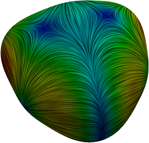
  $r(\phi , \theta ) = 1 + r_0\cos (\phi )\sin (3\theta )$. Figure 1 shows the evolution for $r_0 = 0.4$ and zero initial velocity. The dynamics of the induced tangential flow field and shape changes are clearly visible. The correspondence between $\boldsymbol {v}$ and $\mathcal {V}$ is further highlighted in kinetic energy plots, with a strong increase in normal kinetic energy and an induced but delayed response of the tangent kinetic energy at the beginning. The later relaxation towards a sphere corresponds to a more intermediate coupling. The results correspond to ${Re} = 1$ and ${Be} = 2$, and the simulations are performed with $h = 4.68 \times 10^{-2}$ and $\tau = 4.9\times 10^{-3}$. The dependency on ${Re}$ ( ${Be} = 2$) and ${Be}$ ( ${Re} = 1$) is considered in figure 2. The strongest oscillations are observed for large ${Re}$ and small ${Be}$. However, also for small ${Re}$, the dynamics significantly differs from pure Helfrich flow, which is shown for comparison.

Figure 1. (a) Relaxation of a perturbed sphere for  $t = 0$, $0.25$, $0.5$, $0.75$, $1$,
$1$,  $1.25$, $1.75$, $2$,
$2$,  $2.5$, $7.5$ (left to right, top to bottom); the tangential flow field is visualized by line integral convolution (LIC). Tangent, normal and overall kinetic energy $E_{{T}} := (\int _\mathcal {S}\langle \boldsymbol {v},\boldsymbol {v}\rangle \,\text {d}\mathcal {S})/{2}$, $E_{{N}} := (\int _\mathcal {S}\mathcal {V}^2\,\text {d}\mathcal {S})/{2}$ and $E_{{T}}+E_{{N}}$, respectively, against time $t$ (b) and tangent kinetic energy $E_{{T}}$ against normal kinetic energy $E_{{N}}$ (c).

Figure 2. Deviation from a sphere  $\sigma _{{S}}$ against time $t$ for different Reynolds numbers ${Re}$ (a,b) and Bending capillary numbers ${Be}$ (c,d) for the perturbed sphere simulation (a,c) and power spectrum of the normalized deviation from a sphere $\sigma _{{S}} / \langle \sigma _{{S}}\rangle$ (b,d) with $\langle \sigma _{{S}}\rangle$ the time average of $\sigma _{{S}}$. Pure Helfrich flow is shown for comparison as a dashed line and is indicated as ‘no flow’.
4.2. Killing vector field
The initial tangential velocity on the unit sphere is given by the Killing vector field  $\boldsymbol {v}|_{t=0}=(-z,0,x)^T$ with $\boldsymbol {X}=(x,y,z)^T\in \mathcal {S}$. The tangential velocity induces deformations towards ellipsoidal-like shapes. Due to the induced normal velocity, energy dissipates. Theoretically, a force balance with the bending forces of the Helfrich energy can be established. Using the axisymmetric setting, an ordinary differential equation for these meta-stable states can be derived. However, these states can never be reached during evolution. The shape instead overshoots, oscillates and further dissipates energy, which decreases the driving force and leads to a relaxation back to a sphere with zero tangential velocity (see figure 3). The results correspond to ${Re} = 1$ and ${Be} = 2$, and the simulations are performed with $h = 4.68\times 10^{-2}$ and $\tau = 4.9\times 10^{-3}$. Convergence studies with respect to $h$ and $\tau$ are considered, indicating almost second-order convergence in $h$ and first-order in $\tau$. However, also number, time and strength of shape oscillations change with refinement (see figure 3e). The dependency of the dynamics on ${Re}$ ( ${Be} = 2$) and ${Be}$ ( ${Re} = 1$) is shown in figure 4, again with $h = 4.68\times 10^{-2}$ and $\tau = 4.9\times 10^{-3}$. The results are similar to figure 2.

Figure 3. (a) Relaxation of Killing vector field for  $t = 0$, $1.5$, $3.5$, $15$,
$15$,  $20$ (left to right); the tangential flow field is visualized by LIC. (b,c) Contour plot of the sliced geometry in the time interval $[0,10]$ with ascending grey scale indicating increasing time (b) and plot of the $x$-/
$x$-/ $y$-coordinate of the geometry against time $t$ (c). (d,e) Experimental order of convergence (EOC) for different mesh sizes $h$ and time step widths $\tau$ with a constant ratio $h^2/\tau$ and the measure of the error $e := \|\textrm{div}_{\!\mathcal {S}}\boldsymbol {v} - \mathcal {V}\mathcal {H}\|_2$ (d). Deviation from a sphere $\sigma _{{S}}$ against time $t$ with $\sigma _{{S}} := \int _{\mathcal {S}}(\mathcal {H} - \mathcal {H}_{{S}})^2\,\text {d}\mathcal {S}$ and $\mathcal {H}_{{S}}$ the mean curvature of a sphere with equal surface area for different mesh sizes $h$ (e).

Figure 4. Deviation from a sphere  $\sigma _{{S}}$ against time $t$ for different Reynolds numbers ${Re}$ (a,b) and Bending capillary numbers ${Be}$ (c,d) for the Killing vector field relaxation (a,c) and power spectrum of the normalized deviation from a sphere $\sigma _{{S}} / \langle \sigma _{{S}}\rangle$ (b,d) with $\langle \sigma _{{S}}\rangle$ the time average of $\sigma _{{S}}$.
5. Conclusion
With the considered thin film limit, we have provided a new approach to derive the governing equations of fluid deformable surfaces. They consider fluid-like behaviour in the tangential and normal directions beyond the Stokes limit and are supplemented by a Helfrich energy to model solid-like (bending) behaviour in the normal direction. The splitting of the surface velocity into tangential and normal components shows their tight interplay with geometric quantities of the surface. This is known for the rate-of-deformation tensor. However, additional coupling terms are also present in the inertial terms. The considered numerical approach to solve these equations, which combines evolution of geometric quantities with surface finite elements and a general finite element method for tangential tensor-valued surface partial differential equations, is applicable to general surfaces (not restricted to simply-connected surfaces) and shows reasonable convergence properties with respect to mesh size  $h$ (second-order) and time step width $\tau$ (first-order). The computational examples are chosen to demonstrate the coupling between tangential and normal velocities, where in the presence of curvature any shape change is accompanied by a tangential flow and, vice versa, the surface deforms due to tangential flow. The dynamics of the relaxation strongly depends on the fluid and solid properties. However, the simulations also show that Killing vector fields are only possible as meta-stable states, in situations where the viscous force is balanced by the bending force. The only possible stable stationary state in the considered setting is a sphere with zero velocity.
The computational examples can provide benchmark problems for other numerical approaches, which can be extended to the considered model, e.g. Nitschke et al. (Reference Nitschke, Praetorius and Voigt2017), Olshanskii et al. (Reference Olshanskii, Quaini, Reusken and Yushutin2018), Torres-Sanchez, Santos-Olivan & Arroyo (Reference Torres-Sanchez, Santos-Olivan and Arroyo2020), Lederer et al. (Reference Lederer, Lehrenfeld and Schöberl2019). They also form the basis for more complex models, which include coupling with concentration fields for proteins and dependency of  $\mathcal {H}_0$ on concentration in lipid bilayers, or coupling with liquid crystal theory as in Nitschke et al. (Reference Nitschke, Reuther and Voigt2019a) for Erickson-Leslie type models or with Landau-de Gennes theory on surfaces (Nitschke et al. Reference Nitschke, Reuther and Voigt2019b) for Beris-Edwards type models, which also can be extended by active contributions to model, e.g. phenomena as considered in Keber et al. (Reference Keber, Loiseau, Sanchez, DeCamp, Giomi, Bowick, Marchetti, Dogic and Bausch2014). However, any quantitative comparison in these applications will require to also consider the surrounding bulk phases, as, for example, considered in Barrett et al. (Reference Barrett, Garcke and Nürnberg2015a), Barrett et al. (Reference Barrett, Garcke and Nürnberg2015b), or at least a constraint for the enclosed volume. Even if the approach is applicable for general surfaces, it cannot handle topological changes. This would require a reformulation of the equations using an implicit description, e.g. the diffuse interface approach (Rätz & Voigt Reference Rätz and Voigt2006).
Acknowledgements
A.V. was supported by DFG through FOR3013. We further acknowledge computing resources provided by JSC within HDR06 and ZIH at TU Dresden.
Declaration of interests
The authors report no conflict of interest.


 Open access