


1. Introduction
There has been considerable interest in how a stratified ambient affects the stability and dynamics of several canonical flows, such as plane Couette (Facchini et al. Reference Facchini, Favier, Le Gal, Wang and Le Bars2018), plane Poiseuille (Le Gal et al. Reference Le Gal, Harlander, Borcia, Le Dizès, Chen and Favier2021), Taylor–Couette (Molemaker, McWilliams & Yavneh Reference Molemaker, McWilliams and Yavneh2001; Le Bars & Le Gal Reference Le Bars and Le Gal2007) and the Stokes oscillatory boundary layer (Robinson & McEwan Reference Robinson and McEwan1975). The impacts of stable stratification on boundary layer instability and transition have been extensively studied in the context of atmospheric boundary layers. In this setting, the boundary in question has typically been modelled as flat and horizontal, with stationary external forcing (Mahrt Reference Mahrt2014). The stability of boundary layers on inclined walls with a stratified ambient fluid have also been studied, for instance in the experiments of Hart (Reference Hart1971), where a plate forming a lower boundary of a container with linearly stratified fluid was tilted at  $42^{\circ }$ from the horizontal and oscillated in its own plane in the direction of maximum slope. When the forcing amplitude was small and the forcing frequency was comparable to the buoyancy frequency, the boundary layer flow became unstable. Using perturbation analysis, Candelier, Le Dizès & Millet (Reference Candelier, Le Dizès and Millet2012) studied the inviscid stability of stably stratified, non-inflectional, unidirectional stationary boundary layer flows on a wall inclined with respect to gravity. They found the boundary layer flow to be unstable for any inclination, and the growth rate of the instability to be greatest when the wall was vertical, i.e. when the shear and the stratification were orthogonal. Note that their boundary layer flow was horizontal, whereas that in Hart (Reference Hart1971) was in the direction of the inclination. Chen, Bai & Le Dizès (Reference Chen, Bai and Le Dizès2016) studied the viscous stability of a boundary layer flow on a stationary vertical wall in a stably stratified fluid, again with the boundary layer flow in the horizontal direction. Along with the two-dimensional Tollmien–Schlichting instability, they also found a more unstable three-dimensional instability, called radiative instability, resulting from the coupling between the boundary layer shear and internal waves associated with the ambient stratification. The nonlinear evolution and development of the instability was not pursued.
Blanchette, Peacock & Cousin (Reference Blanchette, Peacock and Cousin2008) studied the stability of the boundary layer on the sidewall of a container filled with linearly stratified fluid, moving vertically at a constant velocity (using a conveyor belt rather than a long moving wall). Here the shear in the vertical wall layer was orthogonal to the stratification, but the flow in the layer was also in the vertical direction, was inflectional in the boundary layer, and diminished rapidly with distance normal to the moving wall. This is in contrast to the set-up considered in Chen et al. (Reference Chen, Bai and Le Dizès2016), where the vertical wall was stationary and the forced horizontal bulk flow monotonically came to rest at the wall. Above a critical wall velocity, Blanchette et al. (Reference Blanchette, Peacock and Cousin2008) found the boundary layer to lose stability to a nominally two-dimensional (spanwise invariant) cellular pattern that travelled in the opposite direction to the moving boundary. Once nonlinearly saturated, the cellular structures remained within the boundary layer region.
The experiments of Blanchette et al. (Reference Blanchette, Peacock and Cousin2008) were essentially the zero-frequency analogue of the earlier experiment by Robinson & McEwan (Reference Robinson and McEwan1975), who, like Hart (Reference Hart1971), forced the vertical wall (or rather, a slat covering part of the wall) to oscillate. The resulting boundary flow is a stratification-modified oscillatory Stokes layer. The oscillating slat in the rectangular container is akin to a wavemaker. A rectangular container with a wavemaker at one sidewall is a very commonly used geometry in the laboratory study of internal waves motivated by oceanographic applications (e.g. Gostiaux et al. Reference Gostiaux, Didelle, Mercier and Dauxois2007; Bordes et al. Reference Bordes, Venaille, Joubaud, Odier and Dauxois2012; Dauxois et al. Reference Dauxois, Joubaud, Odier and Venaille2018). The nature of the wavemaker used by Robinson & McEwan (Reference Robinson and McEwan1975) is different (a vertically oscillating flat slat rather than slots oscillating horizontally), but both are deployed in a rectangular container. The other difference between these studies is that Robinson & McEwan (Reference Robinson and McEwan1975) were interested in the instability of the boundary layer rather than the internal wave beams.
The oscillatory Stokes boundary layer flow in a homogeneous fluid is very stable, at least in idealized semi-unbounded settings (von Kerczek & Davis Reference von Kerczek and Davis1974; Blennerhassett & Bassom Reference Blennerhassett and Bassom2008). However, for a flow subjected to a stable buoyancy stratification, Robinson & McEwan (Reference Robinson and McEwan1975) found an unexpected (and up to now unaccounted for) instability with a distinctive pattern of oblique waves in the oscillatory boundary layer. Figure 1 includes a reproduction of their experimental observation of these oblique waves. Von Kerczek & Davis (Reference von Kerczek and Davis1976) tried to study the stability of this flow, but at the time, the complexities of the Floquet analysis of the confined experimental flow were challenging, and several idealizations were needed. These included assuming the base flow to be unidirectional, the instability modes to be spanwise invariant and the vertical direction to be periodic. These idealizations, in particular the spanwise invariance, precluded any consideration of the observed oblique modes. In the present study, we use direct numerical simulations to study the fully nonlinear three-dimensional flow corresponding to the experiments of Robinson & McEwan (Reference Robinson and McEwan1975), maintaining the effects of confinement.

Figure 1.  $(a)$ Schematic of the rectangular cavity filled with a stably stratified fluid; the (blue) slat oscillates vertically in the $z$ direction with non-dimensional amplitude $\alpha$ and frequency $\omega$. Gravity points in the negative $z$ direction. $(b)$ Image from Robinson & McEwan (Reference Robinson and McEwan1975), using a 30.5 cm f/8 schlieren system aligned normal to the slat; flow conditions correspond to buoyancy number $ {\textit {RN}}=3\times 10^{5}$, Prandtl number $ {\textit {Pr}}\approx 700$, forcing frequency $\omega =0.87$ and forcing velocity amplitude $\alpha \approx 0.02$.
Even in the absence of stratification, confinement effects are important: the oscillatory Stokes layer in a confined cavity is rolled up by the orthogonal endwalls (Vogel, Hirsa & Lopez Reference Vogel, Hirsa and Lopez2003). The resulting rollers tend to fill the cavity and are prone to instability, primarily breaking the half-period-flip symmetry (Blackburn & Lopez Reference Blackburn and Lopez2003b; Leung et al. Reference Leung, Hirsa, Blackburn, Marques and Lopez2005; Blackburn, Marques & Lopez Reference Blackburn, Marques and Lopez2005). This spatiotemporal symmetry-breaking has much in common with the instabilities of the von Kármán vortex street in the wake of a cylinder (Blackburn & Lopez Reference Blackburn and Lopez2003a; Marques, Lopez & Blackburn Reference Marques, Lopez and Blackburn2004). Of particular interest here are the modulated travelling wave modes that are aligned obliquely to the rollers. Is there a connection with the oblique modes reported in Robinson & McEwan (Reference Robinson and McEwan1975)? This is not clear. What is clear is that stratification completely destroys the rollers. In a two-dimensional setting, only planar internal wave beams are admitted into the cavity along the characteristics of the stratified medium (Wu, Welfert & Lopez Reference Wu, Welfert and Lopez2018). What happens in three dimensions, especially when the oscillating boundary has a span which is a fraction of the span of the container, as in the experiments of Robinson & McEwan (Reference Robinson and McEwan1975), is addressed here.
2. Flow configuration and governing equations
The flow system shown schematically in figure 1 mimics the geometry and parameter regimes explored experimentally in Robinson & McEwan (Reference Robinson and McEwan1975); also shown is a schlieren image of the oblique waves from their experiment. A rectangular container of height  $h$, span $s$ and length $\ell$ is filled with a fluid of kinematic viscosity $\nu$, thermal diffusivity $\kappa$ and coefficient of volume expansion $\beta$. All four vertical walls are insulated (zero flux) and the top and bottom walls are maintained at constant temperatures, with the top hotter than the bottom; their temperature difference is $\Delta T$. All walls are no-slip and stationary, except for the ‘front’ wall, which has a centred slat of width $s/2$ that oscillates vertically with angular frequency $\varOmega$ and maximal velocity $W$. Gravity $g$ acts in the downward vertical direction. If the slat is stationary, the fluid is stably linearly stratified. The system is non-dimensionalized using $h$ as the length scale and $1/N$ as the time scale, where $N=\sqrt {g\beta \Delta T/h}$ is the buoyancy frequency. A Cartesian coordinate system $\boldsymbol {x}=(x,y,z)\in [-0.5s/h,0.5s/h]\times [0,\ell /h]\times [-0.5,0.5]$ is fixed with its origin at the centre of the front wall, and the corresponding velocity is $\boldsymbol {u}=(u,v,w)$. The governing Navier–Stokes–Boussinesq equations are
 \begin{equation} \left. \begin{aligned} \boldsymbol{u}_t + (\boldsymbol{u}\boldsymbol{\cdot}\boldsymbol{\nabla})\boldsymbol{u} & ={-}\boldsymbol{\nabla} p + \varTheta\hat{\boldsymbol{z}} + \frac{1}{{\textit{RN}}}\nabla^2 \boldsymbol{u},\\ \varTheta_t + (\boldsymbol{u}\boldsymbol{\cdot}\boldsymbol{\nabla}) \varTheta & ={-}w+\frac{1}{{\textit{Pr}}\,{\textit{RN}}}\nabla^2 \varTheta, \quad \boldsymbol{\nabla}\boldsymbol{\cdot}\boldsymbol{u}=0, \end{aligned} \right\} \end{equation}
where  $p$ is the total pressure, $\varTheta =T-z$ is the deviation temperature, $ {\textit {RN}} = N h^2/\nu$ is the buoyancy number and $ {\textit {Pr}}=\nu /\kappa$ is the Prandtl number. The non-dimensional vertical velocity of the slat is $w=\alpha \sin (\omega t)$, with forcing velocity amplitude $\alpha =W/N h$ and frequency $\omega =\varOmega /N$. The non-dimensional peak-to-peak vertical displacement of the slat then is $2\alpha /\omega$.
The geometry used in Robinson & McEwan (Reference Robinson and McEwan1975) had aspect ratios  $s/h\approx 1.5$ and $\ell /h\approx 0.38$, whereas we use $s/h=1$ and $\ell /h=1/3$. They used salt rather than temperature as the stratifying agent. It was suggested by von Kerczek & Davis (Reference von Kerczek and Davis1976) that the observed instabilities were due to the large Prandtl number of salt. To test this, we consider Prandtl numbers $ {\textit {Pr}}=0.7$ (air), $ {\textit {Pr}}=7$ (water), $ {\textit {Pr}}=70$ (silicon oil) and $ {\textit {Pr}}=700$ (analogous to salt water stratification), as well as $ {\textit {Pr}}=1$. The strength of the stratification is quantified by $ {\textit {RN}}$. The experiments of Robinson & McEwan (Reference Robinson and McEwan1975) were conducted with $ {\textit {RN}}\approx 2\times 10^{5}$ and $3\times 10^{5}$; all simulations presented here have $ {\textit {RN}}=3\times 10^{5}$. We limit the discussion to two forcing frequencies: $\omega =0.87$, at which the experiments report oblique waves, and $\omega =0.51$, where oblique waves are not observed experimentally. The top and bottom boundary conditions also differ between the experiments and our simulations. Using salt stratification, the bottom wall in the experiment has zero flux, and so a stratification purely linear in $z$ is impossible. Also, in the experiments the top surface was open to the air rather than a rigid no-slip lid (issues concerning the meniscus and contact line dynamics at the vertically oscillating slat were not discussed).
The system symmetries are a vertical half-period-flip,  $\mathcal {H}_z$, and a spanwise reflection, $\mathcal {K}_x$; their actions are
 \begin{equation} \left. \begin{aligned} & \mathcal{H}_z: [u,v,w,\varTheta](x,y,z,t)\mapsto[u,v,-w,-\varTheta](x,y,-z,t+{\rm \pi}/\omega),\\ & \mathcal{K}_x: [u,v,w,\varTheta](x,y,z,t)\mapsto[{-}u,v,w,\varTheta]({-}x,y,z,t). \end{aligned} \right\} \end{equation}
 The governing equations are solved using a Chebyshev pseudo-spectral code which has been used to study other oscillatory forced stratified flows (Yalim, Lopez & Welfert Reference Yalim, Lopez and Welfert2018; Yalim, Welfert & Lopez Reference Yalim, Welfert and Lopez2019; Yalim, Lopez & Welfert Reference Yalim, Lopez and Welfert2020; Grayer et al. Reference Grayer, Yalim, Welfert and Lopez2020, Reference Grayer, Yalim, Welfert and Lopez2021; Buchta et al. Reference Buchta, Yalim, Welfert and Lopez2021). Up to  $161$ Chebyshev collocation points in each of the three spatial directions and $1000$ time steps per forcing period were used. The initial conditions used were either starting from rest or starting from a solution at a lower $\alpha$ for given $ {\textit {RN}}$, $ {\textit {Pr}}$ and $\omega$. The vertical velocity on the slat wall ( $y=0$) is regularized, as in Lopez et al. (Reference Lopez, Welfert, Wu and Yalim2017), from an oscillating step function to
 \begin{equation} w(x,0,z,t) = r_x(x)\,r_z(z)\,\alpha\,\sin(\omega t), \end{equation}
where
 \begin{equation} r_x(x) =\frac{1}{2}\left[ \tanh\frac{x+0.25}{\delta} -\tanh\frac{x-0.25}{\delta} \right] \quad \text{and}\quad r_z(z) = 1 - 2e^{{-}1/2\delta} \cosh\left(\frac{z}{\delta}\right), \end{equation}
with  $\delta =0.02$.
3. Response flows
For forcing velocity amplitudes  $\alpha$ below some critical value $\alpha _c$ (which depends on $\omega$, $ {\textit {Pr}}$, $ {\textit {RN}}$ and the aspect ratios), the response is a synchronous symmetric limit cycle. Figure 2 shows snapshots in three planes of the vertical gradient of the deviation temperature, $\varTheta _z$, at $ {\textit {RN}}=3\times 10^{5}$ and $\alpha =10^{-4}$, for $\omega =0.51$ (top row) and $\omega =0.87$ (bottom row), at various $ {\textit {Pr}}$. For the large $ {\textit {RN}}$ considered, the flow is largely unaffected by $ {\textit {Pr}}$ for $ {\textit {Pr}}>1$. For $ {\textit {Pr}}>1$, viscous diffusion, controlled by $1/ {\textit {RN}}$, dominates over thermal diffusion, controlled by $1/ {\textit {Pr}} {\textit {RN}}$. For forcing velocity amplitudes $\alpha$ below critical ( $\alpha _c\sim {\mathcal {O}}(\times 10^{-2})$ in this parameter regime), the response flows at a given forcing frequency $\omega$ scale with $\alpha$. The kinetic energy scales with $\alpha ^2$, whereas the kinetic energy of the mean flow scales with $\alpha ^4$. For very small $\alpha$, the mean flow is extremely weak, but since it grows faster with $\alpha$, at a critical $\alpha$ the synchronous limit cycle becomes unstable, breaking one or both of the symmetries.

Figure 2. Snapshots at maximal vertical velocity of the slat, showing plane sections of  $\varTheta _z$ of the symmetric limit cycle for $ {\textit {RN}}=3\times 10^{5}$, $\alpha =10^{-4}$, with $ {\textit {Pr}}$ as indicated for $(a)$
$(a)$  $\omega =0.51$ and $(b)$
$(b)$  $\omega =0.87$. The locations of the planar slices, indicated by magenta lines, are $x=0$ (vertical streamwise midplane), $y=0.01$ (vertical, spanwise in the slat boundary layer) and $z=1/\sqrt {8}$ (horizontal, at roughly 3/4 height).
The vertical oscillation of the slat creates momentum imbalances along edges of the slat. At low forcing velocity amplitude, these imbalances are mostly confined to the top and bottom edges of the slat, where it meets the horizontal walls of the container. As a result, these edges are sources of vorticity and emit wave beams carrying energy away from the slat. Along the top and bottom horizontal edges,  $(x,y,z)=(x,0,\pm 0.5)$ with $|x|\le 0.25$, the beams are directed at angles $\varphi =\mp \cos ^{-1}\omega$ relative to the vertical. At large $ {\textit {RN}}$, the angles are essentially determined by the inviscid dispersion relation for internal waves in a linearly stratified medium, independently of $ {\textit {Pr}}$ (Sutherland Reference Sutherland2010). The beams emanating from these edges propagate in the interior, forming a pair of planar vortex sheets, while beams emanating from the corners at $(x,y,z)=(\pm 0.25,0,\pm 0.5)$ propagate along rays of cones, forming quarter-conical vortex sheets that merge smoothly with the planar sheets. The vortex sheet emitted from the top is a half-period out of phase with that emitted from the bottom, due to the vertical oscillation of the slat.
At sufficiently large  $ {\textit {RN}}$, the wave beams originating from the edges are only weakly damped as they propagate along straight lines, and eventually reflect on the walls of the container. The reflection laws for internal waves in stratified fluids are similar to those for inertial waves in rotating fluids, and are in general different from standard Euclidean reflection laws (Phillips Reference Phillips1963; Wu, Welfert & Lopez Reference Wu, Welfert and Lopez2020), unless the reflecting surface is parallel or perpendicular to the direction of stratification (or the axis of rotation), as is the case here for all walls of the container. Figure 2 illustrates the patterns of the beams in three planes, $x=0$ (vertical streamwise midplane), $y=0.01$ (vertical, spanwise in the slat boundary layer) and $z=1/\sqrt {8}$ (horizontal, at roughly 3/4 height), at two forcing frequencies $\omega$. For $\omega =0.51$ and $\omega =0.87$, the beams form angles $\varphi \approx \pm 59.3^{\circ }$ and $\varphi \approx \pm 29.5^{\circ }$, respectively, with the vertical direction. This is most obvious in the streamwise midplane, showing the mid-cross-sections of the planar structure of the vortex sheets emitted from the top and bottom edges of the slat. At both these frequencies, the beams are nearly retracing (in the linear inviscid setting, they would be retracing for $\omega \approx 0.5145$ and $\omega \approx 0.8321$), reflecting a number of times off the back and front walls before reaching a corner. The planar structure of the vortex sheets within the width of the slat is manifested by their near spanwise invariance in this region in the horizontal cut at $z=1/\sqrt {8}$. The vertical plane $y=0.01$ shows the impact of the planar sheets reflected off the back wall and impacting the front wall in the region of the slat. Also evident are the traces of the conical sheets from the corners. However, these are much weaker at the low forcing velocity amplitude used ( $\alpha =10^{-4}$).
As noted above, the basic state response flows for  $\alpha <\alpha _c$ have magnitudes of $\boldsymbol {u}$ and $\varTheta$ that scale linearly with $\alpha$. The flows are never unidirectional, even for exceedingly small $\alpha$. The vertical oscillation of the slat produces horizontal temperature gradients in the slat-normal $y$ direction within the boundary layer (but not directly at the boundary, since it is insulating), as isotherms are dragged along by the oscillating slat. This leads to a baroclinic production of vorticity in the spanwise $x$ direction. Additionally, because the width of the slat is shorter than the width of the front wall, there are also horizontal temperature gradients in the $x$ direction at the edges of the slat, since the temperature on the stationary parts of the front wall remains essentially constant whilst the temperature on the slat, at any given height $z$, oscillates. These horizontal temperature gradients lead to a baroclinic production of vorticity in the $y$ direction, and so the vorticity vector is not solely pointing in the spanwise direction, as it would in an idealized two-dimensional spanwise invariant setting. Note that even if the slat extended the entire width of the front wall, there would also be horizontal temperature gradients in the $x$ direction due to the temperature on the lateral walls of the container remaining essentially constant. Furthermore, the spanwise gradients in the vertical velocity, $\partial w/\partial x$, in the regions where the stationary front wall and the oscillating slat meet also contribute to the $y$ component of vorticity. This all results in non-zero helicity density, $H=\boldsymbol {u}\boldsymbol {\cdot }(\boldsymbol {\nabla }\times \boldsymbol {u})$, in the slat boundary layer. Its magnitude scales with $\alpha ^2$ (for a unidirectional flow, the helicity density is identically zero: vorticity is orthogonal to velocity).
Figure 3 illustrates  $\varTheta _z$ (top row) and $H$ (bottom row) for the flows at $ {\textit {Pr}}=7$ and $\omega =0.87$ as $\alpha$ is increased from below to above $\alpha _c$. The flows obtained at $\alpha =0.01$ up to $\alpha =0.018$ remain very similar to the $\alpha =10^{-4}$ flow (see figure 2 for $ {\textit {Pr}}=7$). The $\varTheta _z$ contours in the various planes are spatially similar, and their magnitudes increase linearly with $\alpha$. The helicity density plots show that the response in the bulk away from the slat boundary layer continues to behave like planar waves with zero helicity density. In the slat boundary layer, helicity density grows with $\alpha ^2$. Figure 4 $(a)$ gives a three-dimensional perspective showing isosurfaces of $\varTheta _z$ and $H$ for the $\alpha =0.018$ flow, and supplementary movie 2 includes an animation of these over one forcing period. These, together with figure 3, illustrate the $\mathcal {K}_x$ and $\mathcal {H}_z$ invariances of the base flow response.

Figure 3. Plane sections of  $(a)$
$(a)$  $\varTheta _z$ and $(b)$
$(b)$  $H$ at $ {\textit {RN}}=3\times 10^{5}$, $ {\textit {Pr}}=7$, forcing frequency $\omega =0.87$ and forcing velocity amplitudes $\alpha$ as indicated. The instantaneous snapshots are shown at the maximal vertical velocity of the slat. The locations of the planar slices, indicated by magenta lines, are $x=0$ (vertical streamwise midplane), $y=0.01$ for $\varTheta _z$ and $y=0.005$ for $H$ (vertical, spanwise in the slat boundary layer), and $z=1/\sqrt {8}$ (horizontal, at roughly 3/4 height). Supplementary movie 1, available at https://doi.org/10.1017/jfm.2021.1102, animates the $\alpha =0.0195$ case over one forcing period.

Figure 4. Snapshots at maximal vertical velocity of the slat, showing isolevels  $\varTheta _z=\pm \alpha$ and $H=\pm \alpha ^2$ for $ {\textit {RN}}=3\times 10^{5}$, $ {\textit {Pr}}=7$, $\omega =0.87$, at $(a)$
$(a)$  $\alpha =0.0180$ and $(b)$
$(b)$  $\alpha =0.0195$. Supplementary movie 2 animates the responses over one forcing period.
Increasing  $\alpha$ above 0.018 leads to the breaking of these two symmetries. Figure 3 also includes the planar cuts of $\varTheta _z$ and $H$ at $\alpha =0.019$ and $\alpha =0.0195$, from which the oblique waves in the slat boundary layer are clearly evident and bear a striking resemblance to the experimental waves (see figure 1 $b$). Supplementary movie 1 animates the planar cuts of $\varTheta _z$ and $H$ over one forcing period for $\alpha =0.0195$. Figure 4 $(b)$ and supplementary movie 2 further illustrate the $\alpha =0.0195$ flow. The spanwise reflection $\mathcal {K}_x$ is clearly broken; the breaking of the spatiotemporal $\mathcal {H}_z$-symmetry is more subtle, as the response flow is no longer synchronous with forcing. It is now quasiperiodic with a second frequency associated with a very slow drift of the oblique wave structure. The figures and movies show that the oblique waves reside in the slat boundary layer. The planar cuts of $\varTheta _z$ in supplementary movie 1 indicate that there are weak emissions from the oblique waves in the boundary layer into the interior flow; these appear to merge with the beams from the upper and lower edges of the slat.
To further explore the slow dynamics associated with the oblique waves, we reduce the Prandtl number from  $ {\textit {Pr}}=7$ to $ {\textit {Pr}}=1$, keeping the other parameters the same: $ {\textit {RN}}=3\times 10^{5}$, $\omega =0.87$ and $\alpha$ varying in the neighbourhood of 0.02. This allows numerical simulations with spatial resolution of $101^3$ instead of $161^3$ collocation points, and 100 instead of 1000 time steps per forcing period, reducing the overall computational cost by a factor of 40. The nature of the oblique waves at $ {\textit {Pr}}=1$ is qualitatively the same, and the quantitative differences are small (thicker boundary layer and larger wavelength of the oblique waves); the oblique wave states are robust and not limited to large-
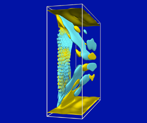
 $ {\textit {Pr}}$ flows. A snapshot of the helicity density at $\alpha =0.02$ is shown in figure 5 $(a)$. For $ {\textit {Pr}}=1$, $\alpha _c\approx 0.0196$, at which the slow modulation period is $\tau _{mod}\approx 1000$ forcing periods, whereas at $\alpha =0.020$ it is $\approx 615$. The behaviour over $\tau _{mod}$ for $\alpha =0.02$ is shown in supplementary movie 3 by strobing $H$ every forcing period in the planes $x=0$, $y=0.005$ and $z=1/\sqrt {8}$. The slow modulation corresponds to drifts in the oblique waves in diagonal directions. The spanwise reflection, $\mathcal {K}_x$, is clearly broken and the solution has a strong bias to the $+x$ side of the slat throughout the entire modulation period. Applying the $\mathcal {K}_x$-symmetry operation at any instant in time and using that as an initial condition results in the $\mathcal {K}_x$-conjugate state, with a strong bias to the $-x$ side. Repeating the simulation, but restricted to the $\mathcal {K}_x$ subspace, results in another oblique wave quasiperiodic state. The corresponding snapshot of $H$ is shown in figure 5 $(b)$. The boundary layer thickness and the oblique wavelength are the same as in the full space, but the $\pm x$ biases are removed, and $H=0$ on the vertical midplane $x=0$. The modulation in the subspace also corresponds to the oblique waves drifting diagonally, but now being $\mathcal {K}_x$-symmetric, their superpositions result in apparent vertical drifts (see supplementary movie 3). Figure 5 $(c)$ shows the power spectral densities of the spanwise velocity at a point, $u(1/\sqrt {8},1/\sqrt {72},1/\sqrt {8},t)$, for the oblique wave solutions in the full space and the $\mathcal {K}_x$ subspace. The spectra are essentially the same for response frequencies at and above the forcing frequency $\omega$. The low response frequencies appear two orders of magnitude lower than $\omega$, and the lowest frequency peak for the full space solution is approximately twice that in the $\mathcal {K}_x$ subspace. For $ {\textit {Pr}}=7$, $\tau _{mod}\approx 150$ at $\alpha =0.0195$ and grows to $\tau _{mod}\approx 4500$ at $\alpha =0.019$; this together with the $\tau _{mod}$ behaviour at $ {\textit {Pr}}=1$ is suggestive of infinite-period bifurcations akin to those observed in periodically-forced Taylor–Couette flow (Lopez & Marques Reference Lopez and Marques2000).

Figure 5. Snapshots at maximal vertical velocity of the slat, showing isolevels of  $H$ for $ {\textit {RN}}=3\times 10^{5}$, $ {\textit {Pr}}=1$, $\omega =0.87$ and $\alpha =0.02$ in $(a)$ the full space and $(b)$ the $\mathcal {K}_x$-symmetric subspace. Supplementary movie 3 shows strobes every forcing period of the full-space helicity density over the slow ${\sim } 10^{3}$-period response. $(c)$ Spectral power density (PSD) of the spanwise velocity at a point, $u(1/\sqrt {8},1/\sqrt {72},1/\sqrt {8},t)$, for the two cases shown in $(a{,}b)$; the response frequency is scaled with $\omega$.
The experimental oblique waves at  $\omega =0.87$ (Robinson & McEwan Reference Robinson and McEwan1975) shown in figure 1 $(b)$ were driven by a peak-to-peak displacement of the slat corresponding to the distance between the two thick black horizontal lines in the middle of the schlieren image. This distance is approximately 2.8 cm and the vertical depth of the fluid in the container is approximately 60 cm, giving a relative total displacement of approximately 0.047. The forcing velocity amplitude for the simulated oblique waves described earlier was $\alpha =0.0195$. This corresponds to a slat total displacement of $2\alpha /\omega =0.045$ over one period. Thus, the experimental oblique waves have been reproduced numerically at the same $ {\textit {RN}}=3\times 10^{5}$, forcing frequency and forcing amplitude, but very different Prandtl numbers (7 compared to 700). Furthermore, the wavelength of the oblique waves, in both the experiment and our simulation, is approximately the total slat displacement (see figures 1 $b$ and 3).
4. Discussion and conclusions
The oblique wave instability of the stratified oscillatory boundary layer observed by Robinson & McEwan (Reference Robinson and McEwan1975) has finally been reproduced numerically in this study, with wavelength and critical forcing amplitude being well matched. The basic state is not unidirectional, and the oscillatory boundary layer has non-trivial helicity. Internal wave beams are driven in the interior for any non-zero forcing amplitude, and their strength (velocity magnitude) increases linearly with the forcing amplitude, whereas the helicity, which resides almost exclusively in the slat boundary layer, increases quadratically with the forcing amplitude. It is possible that interactions between the wave beams and the slat boundary layer trigger the boundary layer instability, leading to the oblique waves. However, the oblique wave instability does not affect the internal waves (at least for  $\alpha$ not too far above critical). The oblique waves appear to introduce very weak disturbances which merge with the internal wave beams in the interior flow. The new frequency introduced by the oblique waves is very low, corresponding to their slow drift; forcing from such a low frequency would introduce wave beams that are almost horizontal. The oblique waves have broken reflection symmetry, and it remains to be determined whether the bifurcation is Hopf-like and local in phase space, or is global in phase space, involving an infinite period. The global bifurcation could be a saddle-node infinite-period or a homo-/heteroclinic collision, or a more exotic bluesky catastrophe (for examples of these and other global bifurcations from experiments and simulations in Taylor-Couette flows, see e.g. Lopez & Marques Reference Lopez and Marques2000, Reference Lopez and Marques2005; Abshagen et al. Reference Abshagen, Lopez, Marques and Pfister2005a,Reference Abshagen, Lopez, Marques and Pfisterb, Reference Abshagen, Lopez, Marques and Pfister2008). The fact that the new period introduced when the oblique waves appear is three orders of magnitude larger than the forcing period constitutes strong prima facie evidence supporting one or more global bifurcation scenarios.
The present system has some similarities to stratified Taylor–Couette flow, which has been extensively used as a well-controlled laboratory experiment to explore the instabilities and dynamics in astrophysical settings, such as accretion disks (Molemaker et al. Reference Molemaker, McWilliams and Yavneh2001; Shalybkov & Rüdiger Reference Shalybkov and Rüdiger2005). The stable stratification in stratified Taylor–Couette flow also inhibits bulk vertical motions, confining vertical motions primarily to the boundary layer on the rotating inner cylinder. Above a critical forcing amplitude (quantified by the inner-cylinder Reynolds number), the boundary layer loses stability to a complex pattern of helical waves with both senses of chirality (Flór et al. Reference Flór, Hirschberg, Oostenrijk and van Heijst2018; Lopez & Marques Reference Lopez and Marques2020, Reference Lopez and Marques2021) – very much in analogy with the oblique wave instability in the present system. Boundary layer flows with strongly stratified exterior bulk flows making the system stiff warrant deeper analysis.
Supplementary movies
Supplementary movies are available at https://doi.org/10.1017/jfm.2021.1102.
Acknowledgements
We thank ASU Research Computing facilities, the Open Science Grid and NSF XSEDE for computing resources.
Declaration of interests
The authors report no conflict of interest.


 Open access