


1. Introduction
Numerical solutions of turbulent flows have been challenging especially under a high-Reynolds-number condition, closely relevant to practical applications in many fields. The wall-bounded turbulent flows are particularly demanding computationally owing to the wide range of temporal and spatial length scales involved, from very large-eddies scaling with the main flow path down to the Kolmogorov micro-scales. Consequently, direct numerical simulations (DNSs) to resolve all turbulence scales are prohibitively expensive for Reynolds numbers of practical interest. The computational cost in terms of mesh count roughly scales with Reynolds number as  $O(R{e^3})$ (Jimenez Reference Jimenez2003) for DNS. Large-eddy simulations (LESs) filtering small scales to be modelled at a sub-grid level are a less costly alternative with generally clear and consistent modelling fidelity (Sagaut & Deck Reference Sagaut and Deck2009). Nevertheless, the mesh count required for LES still scales as $O(R{e^2})$ (Mizuno & Jiménez Reference Mizuno and Jiménez2013), thus the cost of full LES computations, though considerably lower than DNS, is still far too high for wide engineering applications (Jimenez & Moser Reference Jimenez and Moser2000). Even with the projected increase in computer processing power, the challenging situation will remain in the foreseeable future.
Of great relevance and interest is the near-wall region. This is where the turbulence activities are most intense, not only in terms of the level of turbulence but also in terms of the dynamics affecting the overall time-mean flow performance. This is also where the required resolution is the highest owing to the very small spatial and temporal scales of turbulence fluctuations. Being the main culprit of a high-mesh-count requirement, the near-wall region becomes a focal part for which the development of solution approaches with different fidelities and costs has evolved.
A prevalent wisdom based on past observations is that all near-wall turbulence behaves similarly in a self-sustained manner. The seemingly ‘universal’ autonomous behaviour as observed provides a strong impetus to develop a modelled, instead of resolved, treatment for the near-wall turbulent flow region. This consideration leads to the development of the hybrid approach with a scale-resolving outer flow region coupled with a modelled (typically with a Reynolds-averaged Navier–Stokes, RANS, model) near-wall region, notably by the work of Spalart et al. (Reference Spalart, Jou, Strelets and Allmaras1997), as overviewed by Spalart (Reference Spalart2009). The development of wall-modelled LES (Cabot & Moin, Reference Cabot and Moin2000; Piomelli & Balaras, Reference Piomelli and Balaras2002; Larsson, et al., Reference Larsson, Kawai, Bodart and Bermejo-Moreno2016; Bose & Park, Reference Bose and Park2018) makes scale-resolving turbulent flow solutions feasible for various practical applications, though the solution accuracy and applicability are restricted expectedly by the empirical nature of the near-wall RANS modelling as well as by how the transition from a scale-resolving outer flow region to a modelled near-wall region is realized.
Noteworthy is the significant progress in the fundamental understanding of wall-bounded turbulent flows at high Reynolds numbers made in the past decade or so through both advanced experimental measurements and high-resolution DNS analyses. An emerging new consensus recognizes that the near-wall turbulence behaves distinctively with some interesting ‘dual’ characteristics. In addition to the self-sustained ‘universal’ behaviour and dynamics, there is a clear Reynolds-number-dependent part, which seems to be largely passive as influenced by large-scale coherent structures in the outer flow region. An important aspect is the ‘foot-printing’ in the near-wall turbulence by the large coherent structures far away from the wall. The velocity field below the buffer region exhibits clear signatures of the long streaky outflow structures, as revealed in experiment data (Hutchins & Marusic Reference Hutchins and Marusic2007; Marusic, Mathis & Hutchins Reference Marusic, Mathis and Hutchins2010) and DNS results (Bernardini, Pirozzoli & Orlandi Reference Bernardini, Pirozzoli and Orlandi2013; Jimenez Reference Jimenez2013; Agostini & Leschziner Reference Agostini and Leschziner2014; Lee & Moser Reference Lee and Moser2015). The ‘foot-printing’ behaviour is argued to be quasi-steady locally in a very near-wall region (Zhang & Chernyshenko Reference Zhang and Chernyshenko2016; Agostini & Leschziner Reference Agostini and Leschziner2016a). Additionally, the near-wall turbulence seems to be subject to some interactions between local small scales and those large ‘footprints’, through a ‘modulation’ (Mathis, Hutchins & Marusic Reference Mathis, Hutchins and Marusic2009), an aspect subject to some further analyses and discussions (Talluru et al. Reference Talluru, Baidya, Hutchins and Marusic2014; Baars, Hutchins & Marusic Reference Baars, Hutchins and Marusic2017; McKeon Reference McKeon2017; Agostini & Leschziner Reference Agostini and Leschziner2019).
These recent findings on near-wall turbulence have certainly provided some extra challenges to existing modelling approaches and underlying wisdom. Some new wall-modelling efforts are sought to recognize the distinctive scale-dependent behaviour as observed, by generating a synthetic boundary condition to mimic the wall effect (Mizuno & Jiménez Reference Mizuno and Jiménez2013) or super-imposing the traditional ‘universal’ part and the Re-dependent passively influenced part (Marusic et al. Reference Marusic, Mathis and Hutchins2010; Agostini & Leschziner Reference Agostini and Leschziner2016b; Wang, Huang & Xu Reference Wang, Huang and Xu2021). Typically, the modelling efforts of this kind are based on and tested against a single or a small set of DNS data, and the Reynolds number dependency of their applicability remains to be a main issue of interest.
An alternative path, which the present work follows, is aimed at resolving, rather than modelling, the near-wall region, with the use of a small number of fine-mesh blocks, or only a single local fine-mesh block should homogeneity in the two wall-parallel directions be warranted. The primary consideration is that such a locally resolved fine-mesh solution approach must be compatible to the requirement of capturing and resolving the key features as identified in the recent research on near-wall turbulence. In particular, the method needs to capture the large-scale ‘footprints’ and resolve the local scale interactions in the near-wall region adequately.
It is recognized that there have been some previous efforts in developing scale-resolving near-wall turbulent flow in a small local truncated domain. Pascarelli, Piomelli & Candler (Reference Pascarelli, Piomelli and Candler2000) developed a method to couple a global coarse-mesh outer flow domain with a local small fine-mesh near-wall block (often labelled as a ‘minimum flow unit’ (MFU) with direct periodic conditions in the two wall-parallel directions). Their corresponding instantaneous global near-wall flow field is created by mapping the local solution of a small fine-mesh block (MFU) solution directly periodically in space. The resultant instantaneous near-wall flow is thus subject to the artificial signatures of the imposed spatial periodicity with the small block length and width, which are clearly incompatible with the footprints of the outer flow large-scale coherent structures. Tang & Akhavan (Reference Tang and Akhavan2016) adopted a two-domain ‘nested’ system with an MFU fine-mesh block and a coarse-mesh domain for a channel flow. The two domains are solved separately without direct interfacing but coupled by rescaling the flow instantaneously based on spatially averaged quantities. The spatial averaging would smear out any spatial structures in the global domain, thus diminishes the source of the ‘foot-printing’ of the large scales on the local fine-mesh domain. In addition, the coarse-mesh domain in the near-wall region, though rescaled by the fine-mesh solution in the minimal unit domain, would be subject to large discretization errors owing to the under-resolved mesh. Sandham, Johnstone & Jacobs (Reference Sandham, Johnstone and Jacobs2017) developed a method on two distinctively separated scales. The near-wall flow solutions are obtained in discrete non-space filling fine-mesh ‘patches’ which interact with the global coarse-mesh domain by providing instantaneous wall-tangential boundary conditions without any cross-flow to each other. The near-wall coarse-mesh domain is obviously under-resolved. More recently, Carney, Engquist & Moser (Reference Carney, Engquist and Moser2020) focused on non-flow interfacing between a near-wall patch and its global-domain environment. A fringe layer is introduced for which the boundary conditions and a transitional forcing are established based on the time-mean momentum balance. The ability of the near-wall patch in capturing and resolving the self-sustained ‘universal’ dynamics is clearly demonstrated, and the challenges associated with the patch in capturing the large-scale ‘footprints’ are also underlined. A common key limitation suffered by those previous local-domain-based methods seems to arise from the use of a near-wall MFU subject to the spatial periodic conditions, inherently impeding the ‘foot-printing’ by large-scale turbulence structures in an outer flow region. Without the footprints, a ‘modulation’ of near-wall flow would have no starting point.
Given the background, the key intended attributes of the present development are, first, the local fine-mesh domain should directly interact with the outer flow large structures locally and instantaneously to capture the ‘footprints’ appropriately. Second, the local and the global domains are to be coupled in a way to minimize the discretization errors of the under-resolved coarse-mesh near-wall region. A two-scale source-term-oriented approach is adopted to meet these requirements. The original framework is developed for specific multiscale problems of surface micro-structures and effusion cooling (He, Reference He2018). It is realized that the main attributes of the methodology are closely relevant to general wall-bounded turbulent flows. The framework is thus adapted and implemented in an open-source code to examine more general and fundamental cases. The local near-wall fine-mesh block is embedded in a coarse-mesh domain and the embedded block is directly interfaced with its surrounding coarse-mesh. The coupling between the two domains is facilitated by a space–time averaging of the fine-mesh solution over the overlapping coarse-mesh cells. The corresponding residual imbalance can simply be taken as the source terms and mapped to the global coarse-mesh domain. These source terms will effectively balance out the under-resolution-associated errors for the time-averaged solution over the coarse mesh.
A substantive appeal for developing such a local-embedded fine-mesh method is the possibility for much more efficient scale-resolving simulations whilst avoiding taking the wall-modelled route. The potential computational gain will thus need to be measured in terms of the mesh-count scaling with Reynolds number, which in the present context manifests in terms of the fine-mesh block size in relation to the overall mesh count. Of particular relevance is the interface location between the fine- and coarse-mesh domains in the wall-normal direction. Once again, the choice is guided by the scale-dependent outer–inner influence and interaction mechanisms as recently discovered. It is intended that the global coarse-mesh should sufficiently capture and resolve all large-scale turbulence structures, while the near-wall local fine-mesh block is designed to capture both the basic ‘universal’ self-sustaining dynamics and the ‘foot-printing’ of the large scales. It is well recognized that the large coherent structures exist in the log-law region. The correlations (Klewicki, Fife & Wei Reference Klewicki, Fife and Wei2009; Marusic et al. Reference Marusic, Monty, Hultmark and Smits2013) for the low bound of the log-region with respect to Reynolds number would thus provide a physically sound basis for the choice of the interface position.
The rest of the paper is organized as follows. In § 2, we discuss the mesh count scaling with Reynolds number, first for wall-embedded DNS (‘WeDNS’) as the main validations are carried out for DNS. Further scaling analysis is carried out for wall-embedded LES (‘WeLES’) to indicate potential computational gains for practical applications. In § 3, the two-scale methodology is described. A space–time averaging is introduced in either a direct mode or an inverse mode, to be used in the two mesh domains respectively for generating and enacting the source terms. The method implementation and cases set-up for turbulent channel flows will be introduced in § 4. In § 5, the case analyses to assess the validity of the method are presented for DNS channel flow solutions at three Reynolds numbers. In § 6, potential applications of the present method in terms of the Reynolds number scaling are illustrated for LES cases at higher Reynolds numbers. Finally, summary and concluding remarks will be presented.
2. Mesh-count scaling with Reynolds numbers
Given the focus on the near-wall region requiring the highest mesh resolution and the primary intent to facilitate localized fine-mesh blocks, we shall first examine the overall cost implication in terms of the mesh-count scaling with Reynolds number. In this section, the mesh-count estimation will be carried out based on a canonical plane channel flow. As shown in figure 1, a local near-wall fine-mesh block is embedded in a global coarse-mesh domain. The dimensions of the local embedded block are given by the streamwise length  ${l_x}$, the corresponding spanwise width ${l_z}$ and the wall-normal height ${l_y}$, in the x, $z$ and y directions, respectively. In the following, we will first discuss the choice of the embedded fine-mesh block size, and then examine the mesh count–Reynolds number scaling in the context of two-scale DNS and LES solutions.
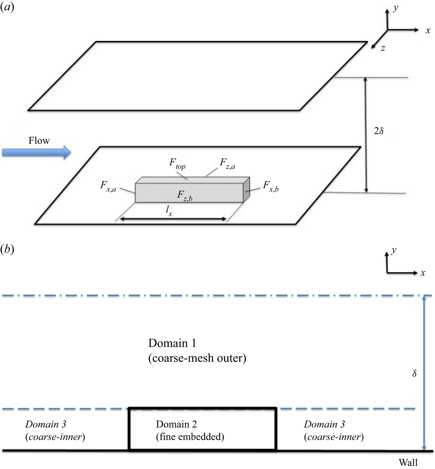
Figure 1. Domain configuration for the channel flow with locally embedded block.
2.1. Sizing fine-mesh block
The selection of the near-wall fine-mesh block size is based on examining the DNS data for an incompressible channel flow by Lee & Moser (Reference Lee and Moser2015) with a range of friction Reynolds numbers up to  $R{e_\tau } = 5200$, where $R{e_\tau } = \; {u_\tau }\delta /\nu $ is based on the wall friction velocity ${u_\tau }$, the boundary layer thickness or the half-channel height $\delta $ and the kinematic viscosity
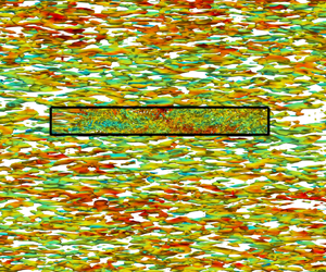
  $\nu $. This is the DNS data set with the highest Reynolds number accessible in the public domain to the authors’ knowledge. The one-dimensional pre-multiplied energy spectra are generated, as shown in figure 2, by accessing and processing the DNS database (https://turbulence.oden.utexas.edu/). The energy spectra present a clear picture of the two distinctive parts of interest: the ‘universal’ first energy peak near the wall and the departing second peak in the outer flow with increasing Reynolds numbers.
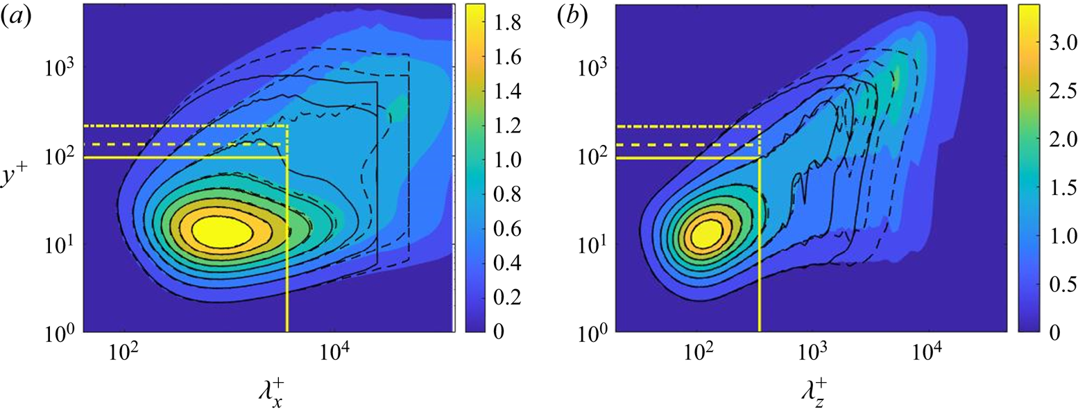
Figure 2. One-dimensional pre-multiplied energy spectra reproduced from DNS data (Lee & Moser Reference Lee and Moser2015) with respect to (a) streamwise and (b) spanwise wavelengths at  $R{e_\tau } \approx 1000$ (solid lines), 2000 (dash lines) and 5200 (shaded contours). The yellow boxes mark the fine-mesh block sizes at $R{e_\tau } \approx 1000$ (yellow solid lines), 2000 (yellow dash lines) and 5200 (yellow dash–dotted lines).
The ‘universality’ of the first peak manifests in terms of the core location at  ${y^ + }\sim 13.5$ independent of Reynolds number, where the superscript ‘+’ indicates the normalization by ${u_\tau }$ and $\nu $ and is referred to as the viscous wall unit. Owing to the dominance of small-scale activities in this inner near-wall region, the energy spectra of the first peak can be covered by constant cut-off wavelengths independent of Reynolds numbers. Based on the desired attribute for the embedded block to capture and resolve the ‘universal’ turbulence behaviour associated with the first peak, we would thus take the block sizes to be constant in wall units in the streamwise and spanwise directions respectively $l_x^ + \approx 3500$ and $l_z^ +{\approx} 350$. The corresponding physical lengths in terms of the overall domain size $(\delta )$ will be reduced with an increase in Reynolds number. The choice of the fine-mesh block sizes in the x and z directions to be constant in wall units is in line with that adopted for a near-wall DNS patch by Carney et al. (Reference Carney, Engquist and Moser2020). The much longer streamwise domain size reflects the near-wall elongated streaky structures in the streamwise direction, consistent with common observations.
In the wall-normal direction, the starting location of the log-law region correlates directly to Reynolds number as  ${y_s} = C{\delta ^ + }^{0.5}$, where $\delta $ is the boundary layer thickness or the channel half-height. In the present work, the coefficient C is taken after Marusic et al. (Reference Marusic, Monty, Hultmark and Smits2013), thus the wall-normal height of the fine-mesh block correlates with the Reynolds number as
 \begin{equation}l_y^ + = 3\sqrt {R{e_\tau }} .\end{equation}
The choice of the embedded block size as described above should suffice in serving the present requirements for the near-wall region: to both resolve the ‘universal’ part of the near-wall turbulence and to capture the ‘foot-printing’ effects of large coherent structures of the outer flow if appropriate interface conditions between the local fine-mesh block and the global coarse-mesh region can be established, as will be introduced in § 3.
2.2. Scaling mesh-count with Reynolds number
For wall-bounded flows, a two-scale consideration leads to different mesh resolution requirements for the near-wall inner part and the outer flow region. We will now examine both DNS and wall-resolved LES. The DNS is considered first because the validations for the concept proof of the present two-scale method are conducted by comparing the present wall-embedded DNS with the well-established full DNS. Then, the LES is considered, as the primary motivation is to develop an efficient alternative to the full wall-resolved LES for practical applications.
First consider a near-wall region to compare LES with DNS. The Kolmogorov micro-scales should be expectedly smaller than a typical mesh resolution of LES in general. The mesh resolution of a wall-resolved LES would however approach that of a DNS in the near-wall region (Moin & Jimenez Reference Moin and Jimenez1997; Jimenez & Moser Reference Jimenez and Moser2000). As such, the mesh resolution required for the near-wall fine-mesh block can be taken to be the same for both DNS and LES in the present work.
For the outer flow region, large-scale flow structures can be captured by a coarser mesh. Given the importance of the history effect for any coherent structures, the mesh needs to cover a global domain of the whole channel. In addition, the mesh resolution required for resolving large turbulence structures should also be much less sensitive to the sub-grid models as well as to numerical dissipations. Hence, a mesh of LES for the bulk flow region can be much coarser than that of a DNS counterpart. It then follows that the main difference in the mesh scaling between a wall-embedded DNS (denoted as ‘WeDNS’) and a wall-embedded LES (denoted as ‘WeLES’) will result from those for the global outer flow region.
2.2.1. Mesh scaling for wall-embedded DNS (WeDNS)
WeDNS scaling is introduced to keep the grid spacings constant in wall units for both the outer global domain and inner near-wall embedded block at different Reynolds numbers for consistency when compared with well-established DNS results. Following the procedure adopted by Jimenez (Reference Jimenez2003), we estimate the mesh count for the near-wall DNS block with its wall-normal height bound by  ${y_s}$ marking the start of the log-law region:
 \begin{equation}NDN{S_{fine\;inner}} = NDN{S_{embed\;block}}\sim \; {N_x}{N_z}\int_0^{y_s^ + } {\frac{{\textrm{d}{y^ + }}}{{\varDelta _y^ + }}} \sim \; {N_x}{N_z}\left( {\frac{{y_s^ + }}{{\varDelta_y^ + }}} \right)\sim \; {\delta ^{ + 0.5}},\end{equation}
where  ${N_x}$ and ${N_z}$ are the mesh count of the fine-mesh block in the x and z directions, respectively, and should be Reynolds number independent, given that the constant cut-off wavelengths in wall units $l_x^ + $ and $l_z^ + $ can be applied as discussed in § 2.1. Furthermore, in the wall-normal y direction, we have $y_s^{+} = l_y^ + {\sim} O({\delta ^ + }^{0.5})$ given by (2.1) and $\varDelta _y^ +{\sim} O(1)$.
For the outer region further away from the wall, the smallest scales to be resolved by DNS are of the order of the larger Kolmogorov scales correlated with the wall distance,  ${\varDelta ^ + }\sim {({y^ + })^{0.25}}$ (Tennekes & Lumley, Reference Tennekes and Lumley1972; Lee & Moser, Reference Lee and Moser2019), and thus
 \begin{equation}NDN{S_{coarse\;outer}}\; \sim \int_{y_s^ + }^{{\delta ^ + }} {{{({\delta ^ + }/{\varDelta ^ + })}^2}\,\textrm{d}{y^ + }/{\varDelta ^ + }\sim {\delta ^{ + 2}}} \int_{y_s^ + }^{{\delta ^ + }} {{y^{ +{-} 3/4}}\,\textrm{d}{y^ + }\sim {\delta ^{ + 2.25}}} .\end{equation}
 The final part to be considered in the present two-scale strategy is the global near-wall region covered by a coarse mesh, apart from that of the fine-mesh block (‘Domain 3’ as indicated in figure 1b). It is assumed that the resolution of this near-wall coarse mesh is comparable to that of the outer coarse-mesh at its low bound interfacing with the fine-mesh block. Thus, a largely constant mesh spacing in this region should be  ${\varDelta ^ + }\sim {(y_s^ + )^{0.25}}$. With the interface position ${y_s}$ fixed by (2.1), we then have
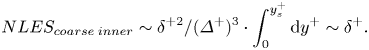
 \begin{equation}NDN{S_{coarse\;inner}}\sim {\delta ^{ + 2}}/{({\varDelta ^ + })^3} \cdot \int_0^{y_s^ + } {\textrm{d}{y^ + }\sim \; {\delta ^ + }^{2.125}} .\end{equation}
The overall mesh count of WeDNS is the sum of all three regions, (2.2)–(2.4). The scaling with Reynolds number is dictated by the highest power index. Thus, the overall mesh count scaling with Reynolds number for the wall-embedded DNS becomes
 \begin{equation}{N_{WeDNS}}\; \sim \; Re_\tau ^{2.25}.\end{equation}
 In contrast, following the same procedure, one should have a Reynolds number scaling of the mesh count for a full DNS as  ${N_{DNS}}\; \sim \; Re_\tau ^3$ (Jimenez, Reference Jimenez2003).
2.2.2. Mesh scaling for wall-embedded LES (WeLES)
As discussed in §2.2.1, the mesh resolution for the near-wall fine-mesh block for WeLES should be identical to that for WeDNS. The mesh count for the near-wall-embedded fine-mesh block will thus be
 \begin{equation}NLE{S_{fine\;inner}} = NDN{S_{embed\;block}}\; \sim \; {\delta ^{ + 0.5}}.\end{equation}
 For the LES outer region, the resolution is no longer set by the Kolmogorov scales as they are supposed to be filtered out and modelled while resolving the large energy-containing scales. Similarly, the outer region starts from the low bound of the log-region  ${y_s}$ and the integral length scales are proportional to the wall distance (Townsend Reference Townsend1976; Jimenez Reference Jimenez2003). With ${y_s}$ again fixed by (2.1), we should have
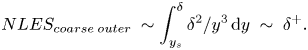 \begin{equation}NLE{S_{coarse\;outer\; }}\sim \int_{{y_s}}^\delta {{\delta ^2}/{y^3}\,\textrm{d}y\; \sim \; {\delta ^ + }} .\end{equation}
 For the large near-wall region covered by a coarse mesh, it is similarly assumed that the resolution of this near-wall coarse mesh is comparable to that of the outer coarse mesh at its low bound. Therefore, the mesh spacing in this region should be  ${\varDelta ^ + }\sim y_s^ + $. We thus have
 \begin{equation}NLE{S_{coarse\;inner}}\sim {\delta ^{ + 2}}/{({\varDelta ^ + })^3} \cdot \int_0^{y_s^ + } {\textrm{d}{y^ + }\sim {\delta ^ + }} .\end{equation}
Summing up all three parts for the overall mesh count, the mesh count scaling with Reynolds number will now be dictated by that of the global coarse meshes for both the outer and inner portions, (2.7) and (2.8). Therefore, the mesh scaling for WeLES should be
 \begin{equation}{N_{WeLES}}\sim R{e_\tau }.\end{equation}
This scaling can also be usefully contrasted to that for a full wall-resolved LES (Jimenez Reference Jimenez2003; Mizuno & Jiménez Reference Mizuno and Jiménez2013):  ${N_{WRLES}}\sim Re_\tau ^2$.
Figure 3 presents the comparison in the mesh count scaling with Reynolds number among several well-established full DNS solutions (Moser, Kim & Mansour Reference Moser, Kim and Mansour1999; Hoyas & Jimenez Reference Hoyas and Jimenez2006; Lozano-Duran & Jimenez Reference Lozano-Duran and Jimenez2014; Lee & Moser Reference Lee and Moser2015), full wall-resolved LES (WRLES) and the present two-scale approach for either a wall-embedded DNS (WeDNS) or a wall-embedded LES (WeLES).
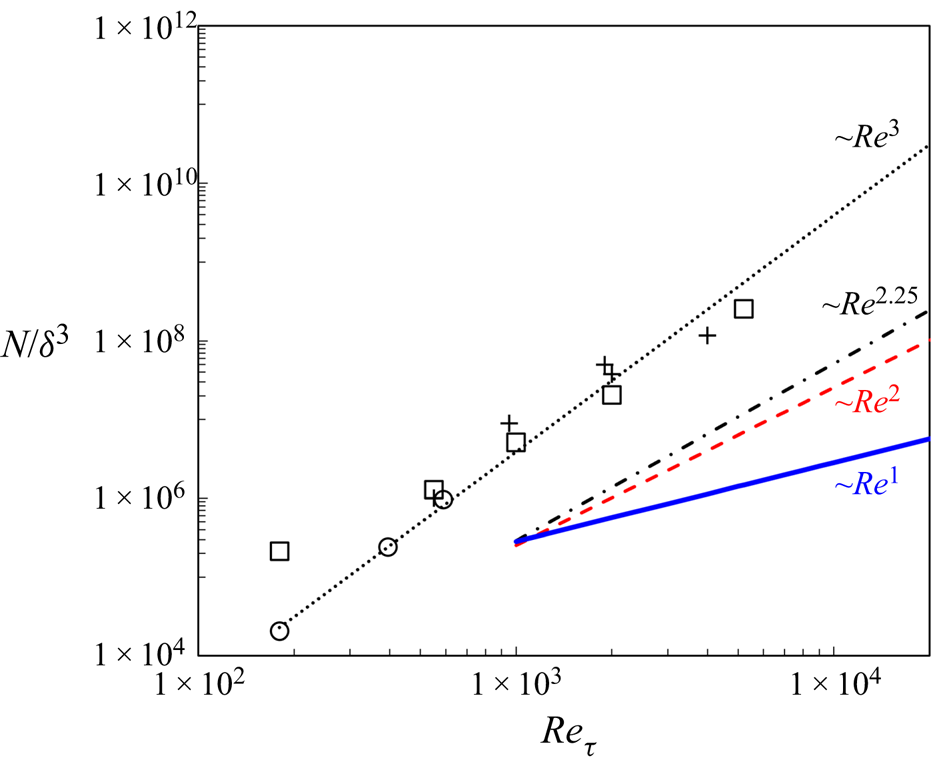
Figure 3. Comparison of mesh count scaling with Reynolds number among full DNS (black dots), full wall-resolved LES (red dash line), the present wall-embedded DNS, ‘WeDNS’ (black dash–dotted line) and wall-embedded LES, ‘WeLES’ (blue solid line). Symbols are for published DNS, ‘□’, Lee & Moser (Reference Lee and Moser2015); ‘+’, Lozano-Duran & Jimenez (Reference Lozano-Duran and Jimenez2014); ‘○’, Moser et al. (Reference Moser, Kim and Mansour1999).
3. Two-scale methodology
A canonical channel flow domain is partitioned, as shown in figure 1. Phenomenologically, the two-scale method needs to be capable of capturing and resolving all key influences and interactions between and within corresponding domains, as indicated in figure 4. First, we assume that the coarse mesh in the global outer domain will be fine enough to resolve coherent large-scale turbulence structures in the log-law region. Thereafter, close attention is paid to two key considerations pertinent to the present work:
(1) the local embedded fine-mesh domain should be able to receive the influence (‘foot-printing’) of the large-scale turbulence structures of outer flow;
(2) the global inner coarse-mesh domain (‘Domain 3’ in figure 1b) is under-resolved, and thus the corresponding discretization errors need to be minimized.
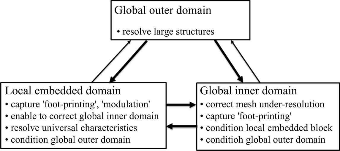
Figure 4. Domain–domain influence and interaction in a two-scale framework.
For item (1), the embedded block will have to be directly interfacing with the global coarse-mesh domain. This will certainly be the case for the top face of the local fine-mesh block ( ${F_{top}}$, as shown in figure 1a). For the upstream and downstream faces ( ${F_{x,a}}$ and ${F_{x,b}}$) and the spanwise side faces ( ${F_{z,a}}$ and ${F_{z,b}}$), direct periodic conditions, as in commonly adopted MFU, are not deemed to be suitable as the resultant periodic flow patterns in the two directions will be clearly incompatible with the large-scale coherent turbulence structures of the outer region, thus impeding the ‘foot-printing’. A key enabler adopted in the present work is a scale-dependent interface method in which the periodic condition is only applied for fine-scale fluctuations. As such, the large scales of the global coarse-mesh region can now directly interact with the local fine-mesh block to capture both the ‘foot-printing’ and the ‘modulation’ effects, as will be described in § 3.1.
For item (2), the correction on the global coarse-mesh domain in the near-wall inner region is enabled by upscaling the fine-mesh solution to the corresponding coarse-mesh cells. The forcing source terms resulting from the upscaling in the local embedded region are then simply mapped to the global inner domain to drive the coarse-mesh solution. The corresponding upscaling method with the source term generation will be described in § 3.2.
3.1. Dual meshing and interface treatment
The local fine-mesh block is created by simply subdividing the corresponding coarse-mesh cells in the near-wall region. This dual-mesh system is purposely introduced to effectively facilitate the interactions between the local embedded fine-mesh block and the global coarse-mesh inner region.
A basic consideration for an interface treatment is the flux conservation. For the present embedded meshing for the fine-mesh block, there will be non-conforming hanging mesh nodes at the interface. The interface conservation is realized through the non-conforming arbitrary mesh interface (AMI) patches based on the Galerkin projection (Farrell & Maddison Reference Farrell and Maddison2011).
Furthermore, two types of interface treatments are considered. For the interface at the top face of the embedded block ( ${F_{top}}$, as marked in figure 1a), the baseline AMI treatment will pass the full flow variable data directly between the coarse-mesh and the fine-mesh sides, effectively by interpolation.
For a pair of side faces (either  ${F_{x,a}}$ and ${F_{x,b}}$, or ${F_{z,a}}$ and ${F_{z,b}}$, as marked in figure 1a), the interface treatment needs to accommodate both the large-scale signatures passed on from the coarse-mesh side, and at the same time, avoid accuracy loss arising from the under-resolution of the coarse mesh. Noting that the fine mesh is effectively a ‘sub-grid’ in relation to the local under-resolved coarse-mesh, we adopt a scale-dependent periodic condition treatment. An instantaneous full flow variable is decomposed into the coarse-mesh resolved local base value and the fine-mesh resolved fluctuation:
 \begin{equation}\boldsymbol{u}(\boldsymbol{x},t) = {\boldsymbol{u}_C}(\boldsymbol{x},t) + {\boldsymbol{u^{\prime\prime}}_f}(\boldsymbol{x},t),\end{equation}
where  ${\boldsymbol{u}_C}(\boldsymbol{x},t)$ is coarse-mesh resolved, obtained based on the baseline AMI. For the fine-mesh fluctuation part ${\boldsymbol{u^{\prime\prime}}_f}(\boldsymbol{x},t)$, the direct spatial periodic condition is applied. For a pair of block side faces (e.g. ${F_{x,a}}$ and ${F_{x,b}}$), we shall thus have
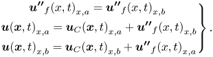 \begin{gather}
\left.\begin{gathered}
{{{\boldsymbol{u^{\prime\prime}}}_f}{{(x,t)}_{x,a}} =
{{\boldsymbol{u^{\prime\prime}}}_f}{{(x,t)}_{x,b}}\; }\\
{\boldsymbol{u}{{(\boldsymbol{x},t)}_{x,a}} =
{\boldsymbol{u}_C}{{(\boldsymbol{x},t)}_{x,a}} +
{{\boldsymbol{u^{\prime\prime}}}_f}{{(x,t)}_{x,b}}}\\
{\boldsymbol{u}{{(\boldsymbol{x},t)}_{x,b}} =
{\boldsymbol{u}_C}{{(\boldsymbol{x},t)}_{x,b}} +
{{\boldsymbol{u^{\prime\prime}}}_f}{{(x,t)}_{x,a}}}
\end{gathered} \right\}.\end{gather}
\begin{gather}
\left.\begin{gathered}
{{{\boldsymbol{u^{\prime\prime}}}_f}{{(x,t)}_{x,a}} =
{{\boldsymbol{u^{\prime\prime}}}_f}{{(x,t)}_{x,b}}\; }\\
{\boldsymbol{u}{{(\boldsymbol{x},t)}_{x,a}} =
{\boldsymbol{u}_C}{{(\boldsymbol{x},t)}_{x,a}} +
{{\boldsymbol{u^{\prime\prime}}}_f}{{(x,t)}_{x,b}}}\\
{\boldsymbol{u}{{(\boldsymbol{x},t)}_{x,b}} =
{\boldsymbol{u}_C}{{(\boldsymbol{x},t)}_{x,b}} +
{{\boldsymbol{u^{\prime\prime}}}_f}{{(x,t)}_{x,a}}}
\end{gathered} \right\}.\end{gather}
Effectively, we have periodic fine-mesh fluctuations for the pairing side faces based on corresponding inhomogeneous instantaneous coarse-mesh variables.
3.2. Two-scale formulations for flow equations
We consider the flow governing equations in a simple form for flow variable vector  $\boldsymbol{u}$:
 \begin{equation}\frac{{\partial \boldsymbol{u}}}{{\partial t}} + R(\boldsymbol{u}) = 0,\end{equation}
which in its original form will be directly solved numerically in the near-wall embedded fine-mesh block and in the global coarse-mesh outer domain as intended. For the global near-wall inner region (‘Domain 3’, figure 1b), a set of augmented flow equations need to be introduced to link the global coarse-mesh solution to the local fine-mesh solution of the embedded block. Upscaling is typically referred to as the way to generate an approximate set of equations for a coarse-scale domain of the same form as those for the fine-scale domain (Farmer Reference Farmer2002). In the present two-scale framework, the upscaling is aimed at producing a coarse-mesh solution which approaches a target solution originated from the fine-mesh domain. In the following, we will first use the commonly known time averaging (Reynolds averaging) as an illustrative example to introduce the upscaling procedure and show how it may be cast in two modes for a fine-scale and a coarse-scale domain. We will then describe how to obtain the upscaled equations for the present work based on space–time averaging.
3.2.1. Upscaling for time averaging/Reynolds averaging
We take a conventional time averaging to illustrate the upscaling with augmented equations. In this case, the fine-scale solution can be taken as a direct time-resolved turbulence solution (or detailed unsteady experimental measurement). For application purposes, we may be interested in a solution with a much lower temporal resolution, and in an extreme but very common case, we may only be interested in the solution with no temporal resolution at all (a time-averaged state). Then, the upscaling from the temporally finely resolved unsteady solution to a steady-state solution for the corresponding time-averaged flow is considered. Take a standard temporal decomposition of an unsteady flow variable into a time-averaged and a fluctuation part:
 \begin{equation}\boldsymbol{u}(\boldsymbol{x},t) = \bar{\boldsymbol{u}}(\boldsymbol{x}) + \boldsymbol{u^{\prime}}(\boldsymbol{x},t).\end{equation}
By time averaging the flow equations (3.3), we have
 \begin{equation}\overline {R(\boldsymbol{u})} = 0.\end{equation}
However, owing to nonlinearity,  $\overline {R(\boldsymbol{u})} \ne R(\bar{\boldsymbol{u}})$, The equations with the time-averaged flow variables can only be balanced with extra terms:
 \begin{equation}R(\bar{\boldsymbol{u}}) = {\boldsymbol{S}_{\boldsymbol{t}}},\end{equation}
where  ${\boldsymbol{S}_{\boldsymbol{t}}}$ is a four-element vector for an incompressible flow. The first element should be zero if the divergence-free criterion is fully achieved for the time-averaged flow. The other elements are three scalars representing the lumped Reynolds stresses in the momentum equations in the three directions, respectively. The augmented equations (3.6) are the upscaled flow equations for the coarse-scale domain, with zero temporal resolution in this case. The lumped form of the Reynolds stresses underlines the simple but fundamental way in which the turbulence stresses affect the time-averaged flow by balancing the corresponding upscaled equations.
The upscaling can be expressed in two modes to be applied in the coarse-scale (denoted with subscript ‘ $C$’) and fine-scale domains (subscript ‘ $f$’). A ‘direct mode’ of the time averaging as applied to the coarse-scale domain simply is
 \begin{equation}R({\boldsymbol{u}_{\boldsymbol{C}}}) = {\boldsymbol{S}_{\boldsymbol{t}}}.\end{equation}
Here the source term  ${\boldsymbol{S}_{\boldsymbol{t}}}$ is taken as the input and the coarse-scale solution ${\boldsymbol{u}_{\boldsymbol{C}}}$ is the output. It then follows that as long as we have a correct source term, regardless of its origin (empirically, experimentally, numerically or analytically), we will get a correct coarse-scale solution as intended. Alternatively, we can view the upscaled equation in an ‘inverse mode’ to be used in the fine-scale domain:
 \begin{equation}{\boldsymbol{S}_{\boldsymbol{t}}} = R(\overline {{\boldsymbol{u}_{\boldsymbol{f}}}} ).\end{equation}
 In this case, a known time-averaged fine-scale solution  $(\overline {{\boldsymbol{u}_{\boldsymbol{f}}}} )$ is taken as the input and the source terms as the output. This is a well-posed problem with the four elements of the source term vector as unknowns and the four flow equations. The source terms are conveniently obtained simply from the flux residual evaluations using the given fine-scale solution. After generating the source terms from the inverse mode (3.8) and driving the coarse-mesh domain to converge, we will have ${\boldsymbol{u}_{\boldsymbol{C}}} = {\bar{\boldsymbol{u}}_{\boldsymbol{f}}}$ as intended.
The inverse mode for a time averaging itself is rarely used as it seemingly does not serve any practical purpose because one will need to get the fine-scale solution in the first place. The possibility of getting a time-averaged solution through an inverse mode is illustrated for self-excited unsteady flows in the context of trailing-edge vortex-shedding (Ning & He, Reference Ning and He2001). As will be shown in the following, however, the inverse mode can be effectively used when the averaging and upscaling are extended to space as well as time.
3.2.2. Upscaling for the present space–time averaging
In the channel flow domain with distinctive two-scale regions, the flow solution of the fine mesh block is first upscaled to the corresponding coarse-mesh cells by a local volume-weighted averaging. For a coarse-mesh cell with m fine-mesh cells, the corresponding local spatially averaged coarse-mesh variable is
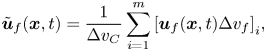 \begin{equation}{\tilde{\boldsymbol{u}}_f}(\boldsymbol{x},t) = \frac{1}{{\Delta {v_C}}}\sum\limits_{i = 1}^m {{{[{\boldsymbol{u}_f}(\boldsymbol{x},t)\Delta {v_f}]}_i}} ,\end{equation}
where  $\Delta {v_C}$ is the volume of the coarse-mesh cell: $\Delta {v_C} = {\sum\nolimits_{i = 1}^m {(\Delta {v_f})} _i}$. Similar to the time averaging, the upscaled equations on the coarse mesh can only be balanced with extra source terms:
 \begin{equation}\frac{{\partial {{\tilde{\boldsymbol{u}}}_f}}}{{\partial t}} + R({\tilde{\boldsymbol{u}}_f}) = {\boldsymbol{S}_{\boldsymbol{s}}}(\boldsymbol{x},t),\end{equation}
where  ${\boldsymbol{S}_{\boldsymbol{s}}}(\boldsymbol{x},t)$ is effectively the source term vector needed to eliminate the spatial discretization errors resulting from the under-resolved coarse mesh to reach the target upscaled solution ${\tilde{\boldsymbol{u}}_f}$ in the coarse-mesh domain. Note that ${\boldsymbol{S}_{\boldsymbol{s}}}(\boldsymbol{x},t)$ is both space and time dependent. Thus, if one simply propagates the spatial averaging associated source terms to the global coarse-mesh domain, there will have to be artificial periodic signatures characterized by the streamwise and spanwise lengths of the embedded block. This is of course to be avoided given the primary intent of the present method development as introduced earlier.
A basic motivating consideration is that for typical wall-bounded turbulent flows, a time-averaged field is much smoother than its unsteady counterpart. Furthermore, for a fully developed channel flow, we effectively have homogeneous statistics in both the streamwise and spanwise directions. This property appeals greatly in relation to propagating the upscaling effect from the local embedded domain to a global one. We thus introduce a space–time averaging to make use of the spatially homogeneous time-averaged flow in the two directions.
For a coarse-mesh cell embedded with m fine-mesh cells, the space–time-averaged flow variable can be simply defined as the local volume average of time-averaged variables of m fine-mesh cells:
 \begin{equation}{\widetilde {\bar{\boldsymbol{u}}}_f}(\boldsymbol{x}) = \frac{1}{{\Delta {v_C}}}\sum\limits_{i = 1}^m {{{[{{\bar{\boldsymbol{u}}}_f}(\boldsymbol{x})\Delta {v_f}]}_i}} .\end{equation}
Noting the averaging being a linear operator, we see that the space–time averaging can be also taken as a time averaging of the volume-averaged coarse-mesh cell as  ${\overline {\tilde{\boldsymbol{u}}} _f}(\boldsymbol{x}) = {\widetilde {\bar{\boldsymbol{u}}}_f}(\boldsymbol{x})$. The upscaled equations in the coarse-mesh domain (‘direct mode’) become
 \begin{equation}\frac{{\partial {\boldsymbol{u}_{\boldsymbol{C}}}}}{{\partial t}} + R({\boldsymbol{u}_{\boldsymbol{C}}}) = {\boldsymbol{S}_{\boldsymbol{st}}}(\boldsymbol{x}).\end{equation}
The source term  ${\boldsymbol{S}_{\boldsymbol{st}}}(\boldsymbol{x})$ is time-independent, thus homogeneous in x and z directions. It consists of two parts:
 \begin{equation}{\boldsymbol{S}_{\boldsymbol{st}}} = {({\boldsymbol{S}_{\boldsymbol{st}}})_f} + \; {({\boldsymbol{S}_{\boldsymbol{t}}})_C}.\end{equation}
The first part is generated by applying the ‘inverse mode’ of the space–time averaging to the fine-mesh time-averaged solution:
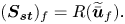 \begin{equation}{({\boldsymbol{S}_{\boldsymbol{st}}})_f} = R({\widetilde {\bar{\boldsymbol{u}}}_f}).\end{equation}
The second part arises from the nonlinear time-averaging effect of the unsteady solution on the coarse-mesh for which needs to be accounted to balance the upscaled equation for the targeted space–time-averaged solution:
 \begin{equation}{({\boldsymbol{S}_{\boldsymbol{t}}})_C} = \overline {R({\boldsymbol{u}_{\boldsymbol{C}}})} - R({\bar{\boldsymbol{u}}_C}).\end{equation}
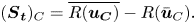
With the source terms as defined in (3.14) and (3.15), when a scale-resolving turbulent flow solution in the coarse-mesh domain is statically converged with a constant time-averaged state, we will get the following by time averaging the upscaled equation (3.12):
 \begin{equation}R({\bar{\boldsymbol{u}}_C}) = R({\widetilde {\bar{\boldsymbol{u}}}_f}).\end{equation}
Hence, the time-averaged coarse-mesh solution  ${\bar{\boldsymbol{u}}_C}$ should converge to the target space–time-averaged fine-mesh solution ${\widetilde {\bar{\boldsymbol{u}}}_f}$ as intended. The time averaging is carried out on-the-fly during the solution (He, Reference He2018).
4. Implementation for channel flow case studies
In this section, the baseline flow solution system will be briefly introduced first. The parameters for both DNS and LES channel flow case studies will then be defined.
4.1. Baseline flow solution method
For concept proof and general application purposes, the two-scale method is implemented in the open source CFD solver OpenFOAM. The present work is focused on the concept proof through case studies for canonical channel flows. The baseline unsteady incompressible flow equations in a channel flow domain  $\varOmega = [0,\; {L_x}] \times [0,\; 2\delta \; ] \times [0,\; {L_z}]\;$ are
 \begin{gather}\left.
{\begin{gathered} {\boldsymbol{\nabla
}\boldsymbol{\cdot }\boldsymbol{u} = 0}\\ {\dfrac{{\partial
\boldsymbol{u}}}{{\partial t}} +
(\boldsymbol{u}\boldsymbol{\cdot }\boldsymbol{\nabla
})\boldsymbol{u} + \dfrac{1}{\rho }\boldsymbol{\nabla }p -
\nu {\nabla^2}\boldsymbol{u} = \boldsymbol{f}} \end{gathered}}
\right\},\end{gather}
\begin{gather}\left.
{\begin{gathered} {\boldsymbol{\nabla
}\boldsymbol{\cdot }\boldsymbol{u} = 0}\\ {\dfrac{{\partial
\boldsymbol{u}}}{{\partial t}} +
(\boldsymbol{u}\boldsymbol{\cdot }\boldsymbol{\nabla
})\boldsymbol{u} + \dfrac{1}{\rho }\boldsymbol{\nabla }p -
\nu {\nabla^2}\boldsymbol{u} = \boldsymbol{f}} \end{gathered}}
\right\},\end{gather}
where  $\boldsymbol{u} = {(u,v,w)^{ - 1}}$. The only non-zero element of the baseline source term vector $\boldsymbol{f}$ is the streamwise pressure gradient, ${f_x} = \textrm{d}P/\textrm{d}\kern0.06em x$. The corresponding boundary conditions for the domain are
 \begin{equation}\left.
{\begin{gathered} {u = 0,\;\textrm{at}\;y =
0\;\textrm{and}\;y = 2\delta }\\
{u\;\textrm{and}\;p\;\textrm{periodic}\;\textrm{in}\;x\;\textrm{and}\;z\;\textrm{directions}\;\textrm{in}\;\varOmega
} \end{gathered}}
\right\}.\end{equation}
\begin{equation}\left.
{\begin{gathered} {u = 0,\;\textrm{at}\;y =
0\;\textrm{and}\;y = 2\delta }\\
{u\;\textrm{and}\;p\;\textrm{periodic}\;\textrm{in}\;x\;\textrm{and}\;z\;\textrm{directions}\;\textrm{in}\;\varOmega
} \end{gathered}}
\right\}.\end{equation}
The flow equations are discretized in a finite-volume scheme, with a second-order central difference scheme in space. The time advancement is achieved by a second-order Crank–Nicolson scheme. A constant time-step is taken in keeping the maximum Courant numbers below 0.5. The pressure-implicit splitting operators (PISO) algorithm is used for solving the incompressible flow field. A flowchart showing the main elements of the present two-scale method, as implemented in the OpenFOAM for incompressible flow, is shown in figure 5.

Figure 5. Flowchart of the two-scale solution process as implemented.
Some extra remarks should be made regarding the source term propagation in the context of capturing the ‘modulation’. In the phenomenological discussions so far, the large-scale coherent structures are regarded effectively as an external forcing from the outflow region originating the foot-printing and the modulation within the embedded near-wall block, which will in turn improve the conditioning of both the global inner coarse-mesh region and the outer flow coarse-mesh region. The related assumption is that those intermediate scales generated and affected by the modulation in the near-wall region should have negligible feedback effects on the large scales in the outer flow region. This assumption is deemed to be justifiable based on the present results, as presented in § 5.1. A simple option to further address this will also be introduced and presented in Appendix A for completeness.
4.2. Parameters for DNS and LES case studies
The implemented two-scale method is applied to a canonical turbulent plane channel flow at  $R{e_\tau } \approx 550$, 1000, 2000, 4100 and 5200. The full computational domain sizes are ${L_x} = 2{\rm \pi} \delta $ and ${L_z} = {\rm \pi}\delta $, where $\delta $ is the half-height of the channel (figure 1). The size of the computational domain corresponds to the minimum one used for the full DNS simulations (Moser et al. Reference Moser, Kim and Mansour1999; Lozano-Duran & Jimenez Reference Lozano-Duran and Jimenez2014). Thorough discussions on the effect of the domain size are made by Lozano-Duran & Jimenez (Reference Lozano-Duran and Jimenez2014), where the same domain size as that used in the present work is proven to be adequate for reproducing one-point statistics of those larger ones. The global domain size is also the same as that adopted by Tang & Akhavan (Reference Tang and Akhavan2016).
The fully developed channel flow is driven by a set mass flow. Given a bulk mean velocity  ${U_b} = (1/2\delta )\int_0^{2\delta } {\bar{u}(y)\,\textrm{d}y} $ in the streamwise direction, the present simulations are carried out at bulk Reynolds numbers in line with those of the published DNS data (Hoyas & Jimenez Reference Hoyas and Jimenez2006; Bernardini et al. Reference Bernardini, Pirozzoli and Orlandi2013; Lee & Moser Reference Lee and Moser2015). The simulations are initialized with a laminar parabolic Poiseuille profile (de Villiers Reference de Villiers2006) and run for sufficiently long time to reach a statistically steady state with mean statistics to differ less than 1 %. The turbulence statistics to be reported are obtained by ensemble-averaging the flow quantities spatially in the two homogeneous directions and in time over at least ten eddy turnover times $\delta /{u_\tau }$.
Uniform grids are implemented in streamwise and spanwise directions. In the wall normal direction (y), grids are allocated with a geometric stretching ratio around 1.05. Within the local embedded DNS region, the mesh grid spacings  $\varDelta x$, $\varDelta y$ and $\varDelta z$ follow the DNS requirement (Bernardini et al. Reference Bernardini, Pirozzoli and Orlandi2013). Given the Kolmogorov scale at wall $\eta _w^ +{\sim} 1.5$, the grid spacing in wall-parallel directions is $\varDelta x/\eta < 7$ and $\varDelta z/\eta < 5$. In the wall normal direction, the largest grid spacing relative to the local Kolmogorov scale is at the interface between the embedded block and the global coarse-mesh region, where ${(\varDelta y/\eta )_{max}}$ is kept below 1.9.
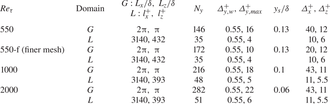
DNS simulations are run for three Reynolds numbers:  $R{e_\tau } \approx 550$, 1000 and 2000, with the details of the simulation parameters given in table 1. Solutions for different mesh densities are also run to examine the mesh sensitivity at $R{e_\tau } \approx 550$, and the result for a refined mesh (denoted as ‘550-f’) is also presented. The DNS results for validations will be presented and discussed in § 5.
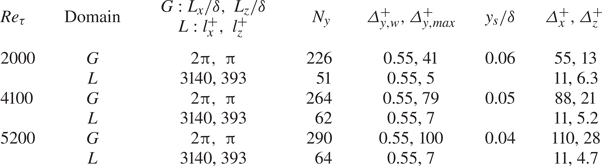
Table 1. WeDNS parameters within global  $(G)$ and local-embedded (L) domains.
Given the interest in developing an efficient method for applications at a moderate to high  $R{e_\tau }$ in the order of at least $O({10^3})$ (Smits & Marusic Reference Smits and Marusic2013), the capability of the two-scale wall-embedded LES (WeLES) is also examined and demonstrated for higher Reynolds number cases, $R{e_\tau } \approx 2000$, 4100 and 5200. For the LES global coarse grids to resolve the energy-containing large scales as intended, the grid spacing follows that of Georgiadis, Rizzetta & Fureby (Reference Georgiadis, Rizzetta and Fureby2010) and the scaling estimated in § 2.2.2. Details of the WeLES simulation parameters are given in table 2. In the present calculations, the explicit sub-grid model is not included, the solutions can thus be regarded as implicit LES where the sub-grid scales are dampened by numerical dissipations. The results of the WeLES simulations will be presented and discussed in § 6.
Table 2. WeLES parameters for global (G) and local-embedded (L) domains.
5. Wall embedded DNS
In this section, the results of the wall embedded DNS will be presented for  $R{e_\tau } \approx 550$, 1000 and 2000 in comparison with the DNS results of Lee & Moser (Reference Lee and Moser2015) and the two-dimensional (2-D) spectral results from the DNS calculations of del Alamo et al. (Reference del Alamo, Jimenez, Zandonade and Moser2004). The emphasis is placed on examining the validity of the present locally embedded two-scale methodology. In particular, attention is paid to the capability of the method in terms of the two major intended attributes: to adequately resolve the ‘universal’ near-wall small scale turbulence dynamics and interactions within the embedded block, and to capture the ‘foot-printing’ of the large-scale structures of the outer flow on the near-wall region.
5.1. Mean statistics
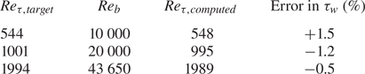
Figure 6 shows the mean velocity profiles in good agreement with the full DNS results. Table 3 presents the predicted wall shear-stresses compared with the values of the published DNS as the target. All the present calculations are set to match the bulk flow Reynolds numbers  $R{e_b}$ of the DNS results. The comparisons between $R{e_{\tau ,computed}}$ and $R{e_{\tau ,target}}$ indicate the accuracy of the wall shear-stress prediction. The errors are all within 2 %.
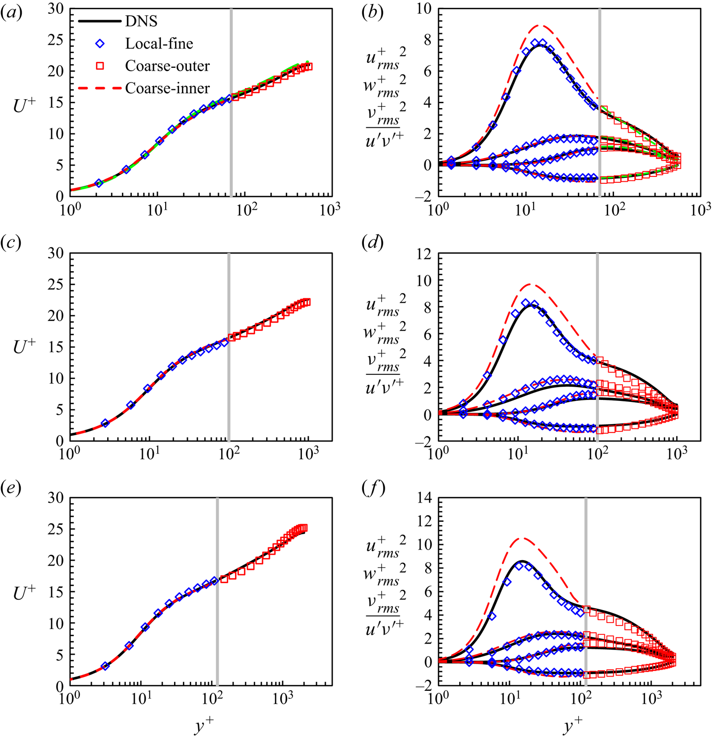
Figure 6. Mean velocity profiles (a,c,e) and turbulence fluctuations (b,d,f) compared with the DNS results (Lee & Moser Reference Lee and Moser2015) marked in black solid lines. The results are at three Reynolds numbers: (a,b)  $R{e_\tau } \approx 550$; (c,d) $R{e_\tau } \approx 1000$; (e,f) $R{e_\tau } \approx 2000$. The blue diamond symbols indicate results within the local fine-mesh block. The red squares and red dashed lines indicate results in the global coarse outer and inner region, respectively. The green dashed lines in panels (a,b) are the results of a finer mesh ‘550-f’ (table 1) in the global region. The vertical grey solid lines mark the interface location ${y_s}$. Note that not all data points are included to increase readability.
Table 3. Wall shear-stress prediction of the two-scale WeDNS approach.
Also shown in Figure 6 are the predicted turbulence intensities and the Reynolds stresses  ${u_{rms}^+}^2$, ${v_{rms}^+}^2$, ${w_{rms}^+}^2$ and ${\overline {u^{\prime}v^{\prime}} ^ + }$ where the subscript ‘rms’ denotes the root-mean-squared values. In general, the local DNS solutions (denoted as ‘Local-fine’) within the local embedded fine-mesh block match well with the full DNS. The coarse-mesh solutions behave differently in the two global regions. In the outer region (denoted as ‘Coarse-outer’), the coarse mesh solutions agree well with the corresponding full DNS both in terms of the mean flow velocities and the turbulence statistics. The results of ‘550-f’ (table 1) with a finer mesh are also presented, which are in good agreement with the standard mesh resolution (‘550’ in table 1). The two solutions from the two meshes of different resolutions are almost indistinguishable in the outer region. The large-scale structures are resolved on the global coarse grids regarding both the mean and the fluctuations. The outer ‘energy plateau’ of the turbulence fluctuations in the streamwise direction is captured by the global coarse-mesh, most clearly at the highest Reynolds number.
For the near-wall region of the global coarse-mesh (‘Domain 3’ as shown in figure 1, denoted as ‘Coarse-inner’), the agreement between the present solution and the reference DNS can only be observed for the time-mean velocities (figure 6a,c,e). It is noted however that the magnitude of turbulence fluctuations in the global near-wall inner region tends to be over-predicted, most noticeably for the streamwise components in figure 6(b,d,f). It should be remarked that the over-riding factor in the global near-wall inner region is the under-resolution of the local coarse-mesh. Lack of sufficiently resolved small scales locally should correspond to lack of dissipation, and thus the over-estimation of the local turbulence fluctuations is expected. Nevertheless, the under-resolved global inner region still serves in receiving the ‘foot-printing’ of the large-scale structures from the outer-flow region, which in turn will feed into the embedded fine-mesh block through the direct interfacing treatment at the coarse mesh resolved level as discussed in § 3.1. The source-term correction of the upscaled flow equations (3.12) is effective only in driving the time-averaged coarse-mesh flow field towards the space–time-averaged target solution of the embedded fine-mesh block. This primary objective of the present work seems to be met adequately, as demonstrated by the comparisons in the mean flow velocity profiles shown in figure 6(a,c,e).
For consistency of the two-scale methodology in the context of the global and local domain partitioning (figure 1b), the correction source terms activated in the global inner domain (‘Domain 3’) arising from the upscaling should approach zero smoothly when approaching from the inner region to the inner–outer interface in the wall-normal direction. Figure 7 presents the distributions of the source terms in the wall-normal direction, for the total source terms  ${S_{st}}$ consisting of the fine-mesh space–time-averaging term ${({S_{st}})_f}$ and the coarse-mesh time-averaging term ${({S_t})_C}$ in (3.13). As can be observed from figure 7, these terms are all decreasing asymptotically to become negligible when approaching the inner–outer interface. This indicates that the global coarse-mesh resolution at the interface is sufficiently fine to resolve the local flow directly. Thus, no corrections should arise from the upscaling around the interface. The diminishing source terms approaching the interface are also in line with the assumption that the feedback from the inner region ‘modulation’ on those large structures in the outer flow region should be negligibly small, as discussed in § 4.1 and further considered in Appendix A. It should be mentioned that the source terms in the spanwise direction, including ${({S_{st}})_{f,z}}$, ${({S_t})_{C,z}}$ and ${S_{st,z}}$, are much smaller than those in the streamwise and wall-normal directions, thus are not shown here.
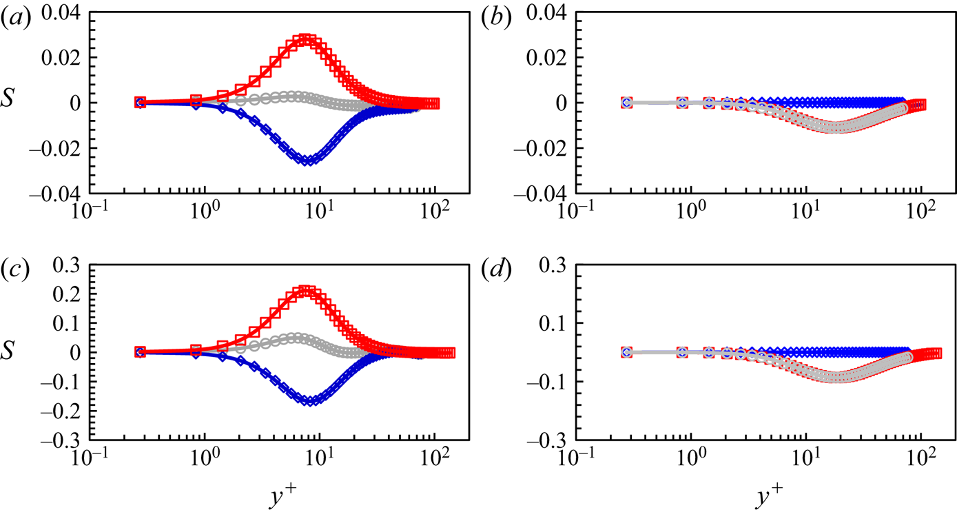
Figure 7. Source term profiles: the fine-mesh space–time-averaging term  ${({S_{st}})_f}$ in blue diamonds, the coarse-mesh time-averaging term ${({S_t})_C}$ in red squares and the total source term ${S_{st}}$ in grey circles, in relation to wall distance ${y^ + }$ at two Reynolds numbers: (a,b): $R{e_\mathrm{\tau }} \approx 1000$; (c,d) $R{e_\mathrm{\tau }} \approx 2000$. (a,c) Source terms in the streamwise direction. (b,d) Source terms in the wall-normal direction.
5.2. Spectral analysis
A key aspect pertinent to the validity and effectiveness of the locally embedded methodology is its ability in capturing and resolving a range of turbulence scales. To examine this, spatial spectral analyses on a near-wall plane are carried out. The wall-normal location commonly taken for such analyses is that around the ‘universal’ first peak of turbulence fluctuations at  ${y^ + } = 13.5$. Figure 8(a) shows the velocity field snapshot on this plane, on which the embedded block is also marked. Two points are worth noting here. First, the large meandering streaky structures are clearly captured by the global near-wall coarse mesh, which in turn feed into the embedded fine-mesh block through the direct interfacing treatment at the coarse-mesh resolved level, as discussed in § 3.1. Thus, the local fine-mesh block will be influenced directly by the large structures captured in the global coarse-mesh domain through both the top interface and the side interfaces (figure 1a). Second, the fine-mesh of the embedded block is enabled to provide a local high resolution effectively thanks to the fine-scale fluctuation based periodic condition (3.2). The two-scale characteristics in the fine-mesh block and the surrounding coarse-mesh region with contrasting resolutions are clearly seen in figure 8(b) indicating corresponding scales of vortical structures and figure 9 showing the near-wall vorticity fields on an x–y plane.
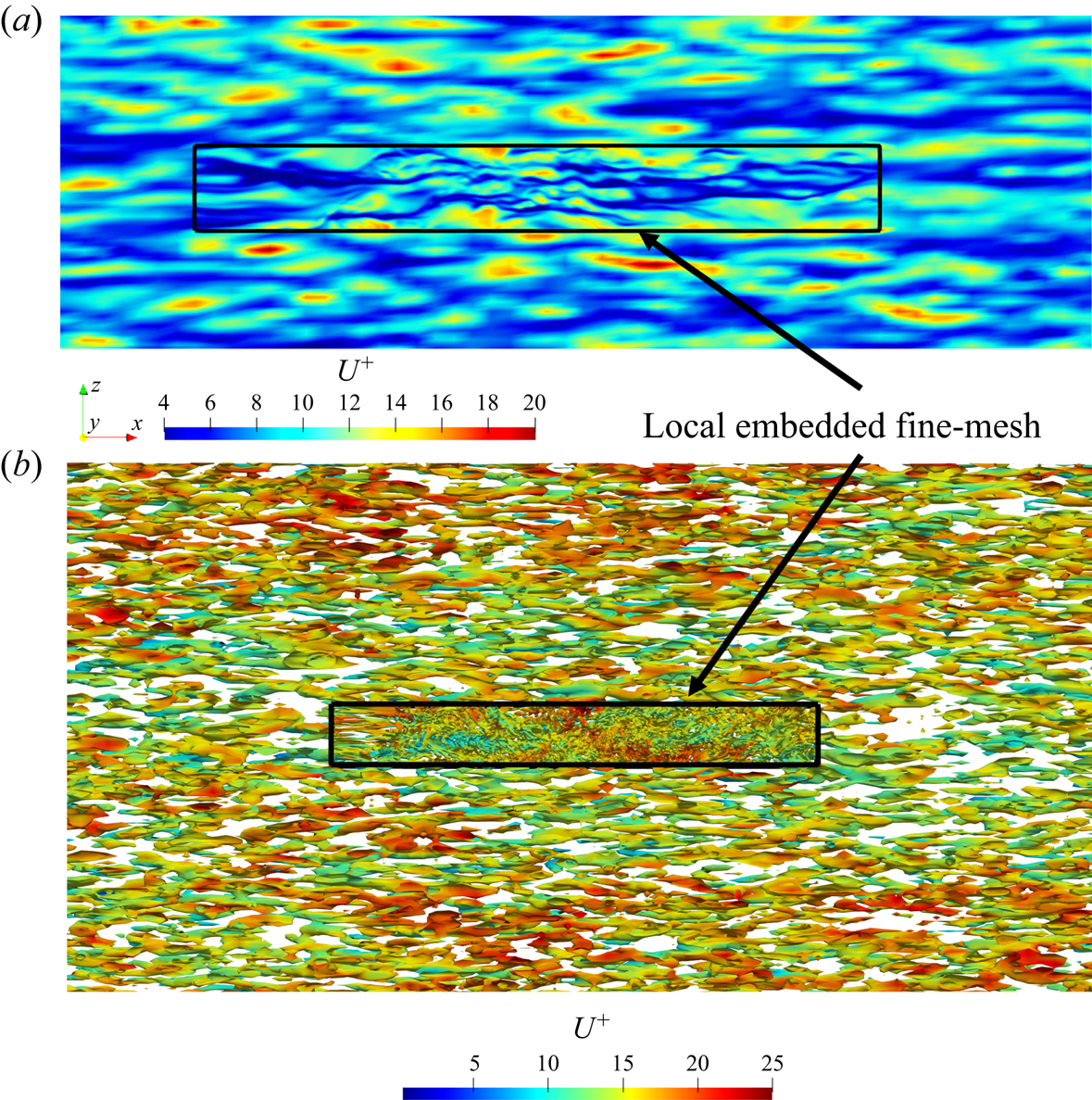
Figure 8. (a) The x–z plane snapshot of the instantaneous velocity field around the embedded block at the inner location  ${y^ + } = 13.5$. (b) Iso-surfaces of the second invariant of the velocity gradient tensor (Jeong & Hussain, Reference Jeong and Hussain1995), coloured with the instantaneous velocity contours. The solid black boxes mark the embedded fine-mesh block.
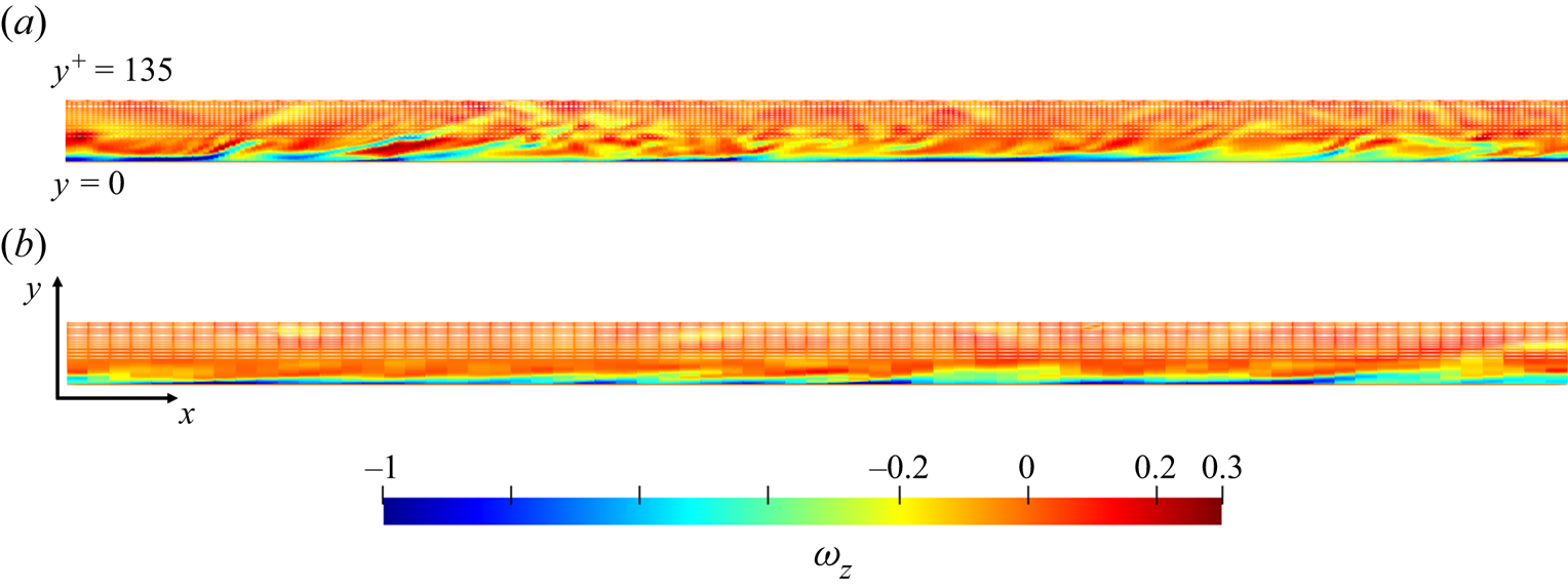
Figure 9. The x–y snapshot of the spanwise vorticity  ${\omega _z}$ contours near wall: (a) the local embedded DNS region; (b) the global coarse-mesh region on the same x–y scale. Contour values are normalized by the maximum magnitude.
Figure 10 shows the one-dimensional streamwise energy spectra. The global coarse-mesh covers adequately the large scales. However, it is clearly under-resolved at higher wave numbers. The profiles of the coarse-mesh spectra deviate from the full DNS, being overpredicted first at intermediate wavenumbers, e.g.  ${k_x} \approx 40$ (figure 10a), and then underpredicted at higher wavenumbers for small scales of the dissipation range. The resolution dependency is more strongly manifested in the energy spectra as functions of the streamwise wavenumbers ${k_x}$ (figure 10a) than those of the spanwise wavenumbers ${k_z}$ (figure 10b). For the high wavenumber part in the spectra, the numerical dissipation caused by the under-resolution of the coarse grids results in a much more abrupt drop of energy (figure 10a). However, the embedded block is sufficiently fine to resolve small scales down to the Kolmogorov ones in the near-wall region, reflected by the predicted spectra at higher wavenumbers. As discussed earlier, the embedded fine-mesh block is able to receive the disturbances of the long wavelength dictated by the global domain size adopted.
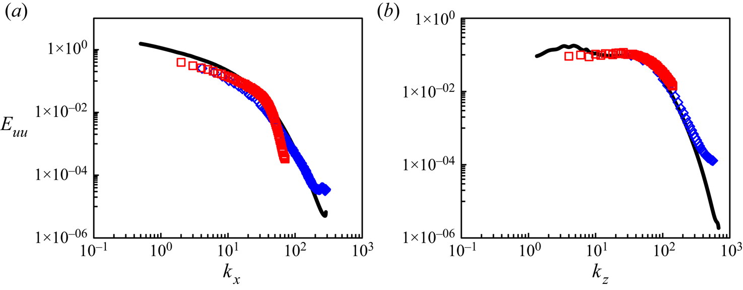
Figure 10. One-dimensional energy spectra at  ${y^ + } = 13.5$ as functions of streamwise wavenumbers ${k_x}$ and spanwise wavenumbers ${k_z}$ compared with DNS results (Lee & Moser Reference Lee and Moser2015) in black solid lines at $R{e_\tau } \approx 1000$. The blue diamond symbols indicate the results within the local fine-mesh block, while the red symbols indicate the results in the global coarse-mesh region.
The most noteworthy feature of the results shown in figure 10 is the overlapping of the two spectra from the fine- and coarse-mesh domains. The smooth overlapping of the two spectra in good agreement with the full DNS indicates that the fine-mesh block is subject to turbulence disturbances of a full spectra range. In contrast, if a global domain solution is indirectly coupled with a small fine-mesh domain with a direct periodic condition (as commonly adopted in MFU), discontinuous spectra from the two domains may occur (Tang & Akhavan Reference Tang and Akhavan2016). A more direct illustration of the length-scale range captured by the fine-mesh solution of the embedded block is provided by a local frequency power spectral density (PSD), as shown in Figure 11, where the dimensionless frequency is taken based on the half-channel height and bulk flow velocity:  $k = f\delta /{U_b}$. It is worth noting that the PSD taken from the middle of the embedded block confirms a full coverage of the spectra range in the locally fine-mesh block. However, the global coarse-mesh region is clearly subject to an underprediction for the small-scale high-frequency part (figure 11) as expected.
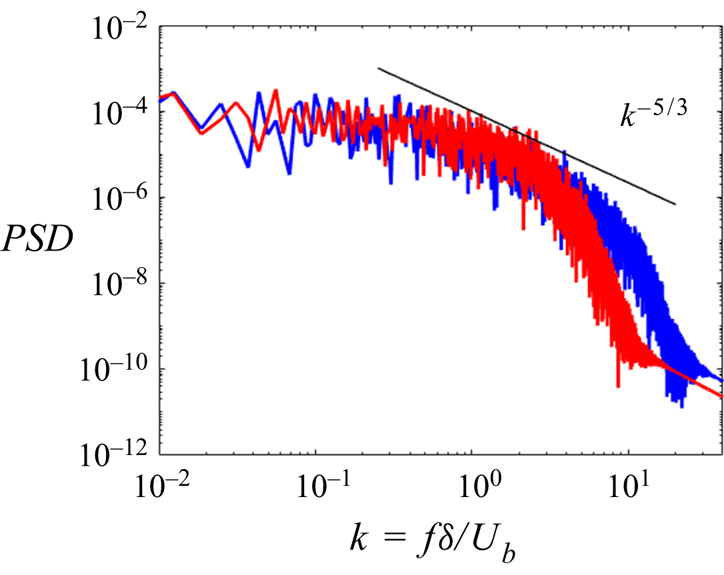
Figure 11. Turbulence power spectra density (PSD) as functions of the non-dimensional frequency at  $R{e_\tau } \approx 1000$. Data obtained at two locations of the same wall normal distance ${y^ + } = 13.5$ at the middle of the embedded fine-mesh block (blue lines) and at a coarse-mesh point outside the embedded block (red lines).
It is emphasized that although the present method is phenomenologically based on a two-scale framework, there is no spectral gap between the two scales assumed, nor is such spectral gap or separation observed in either the spatial spectra from the two domains (figure 10) or the temporal counterparts (figure 11).
Figures 12(a) and 12(c) show the one-dimensional pre-multiplied energy spectra  ${k_z}\varPhi _{uu}^ + $ of the inner embedded DNS region compared with the full DNS results. The counterpart spectra processed from the global coarse-mesh results are shown in figures 12(b) and 12(d) indicating a notable discrepancy in the near-wall region for the dominant shorter-wavelength part. The overprediction of the streamwise velocity fluctuations arising from the local under-resolution in the global inner near-wall region is consistent with the mean statistics, as shown in figure 6. The boxes with the vertical black lines indicate the embedded fine-mesh block size in the spanwise direction. It is clear that the inner ‘universal’ energy peak is sufficiently covered in the embedded block, in line with that illustrated in figure 2. The longer-wavelength disturbances are well captured in the global coarse-mesh domain, as shown in figures 12(b) and 12(d).
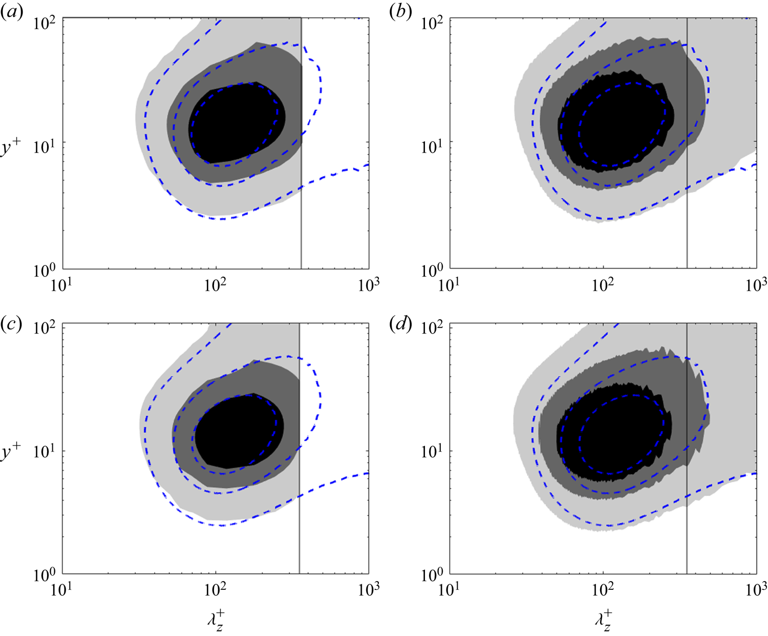
Figure 12. One-dimensional pre-multiplied energy spectra  ${k_z}\varPhi _{uu}^ + $ for the inner region normalized by ${u_\tau }$. (a,c) the present results within the embedded block with the blue dashed lines showing the results from the full DNS database (Lee & Moser Reference Lee and Moser2015); (b,d) the present results of the global coarse-mesh region compared with the same full DNS results. The contour levels are 0.5/1.5/2.5. Results in panels (a,b) are at $R{e_\tau } \approx 1000$. Results in panels (c,d) are at $R{e_\tau } \approx 2000$. Black solid lines indicate the size of the embedded block.
After examining the inner region and the local embedded block, we now evaluate the resolutions in the outer-flow region. Attention is paid to a plane at the outer location  $y_{out}^ + \approx 3.9\sqrt {R{e_\tau }} $, within the log-law region, which is taken by Marusic et al. (Reference Marusic, Mathis and Hutchins2010) as the location where the ‘outer signals’ can be extracted as inputs for their two-scale model. The grid resolution of the global coarse-mesh is examined to see if the local small scales of the large energy-containing structures can be sufficiently resolved. Figure 13 shows the 2-D pre-multiplied energy spectra ${k_x}{k_z}{\varPhi _{uu}}$ in relation to streamwise wavelengths and spanwise wavelengths. As can be seen, the coarse mesh resolves outer large scales down to ${\lambda ^ + } \approx {10^2}$ well in comparison with the full DNS data (del Alamo et al. Reference del Alamo, Jimenez, Zandonade and Moser2004).
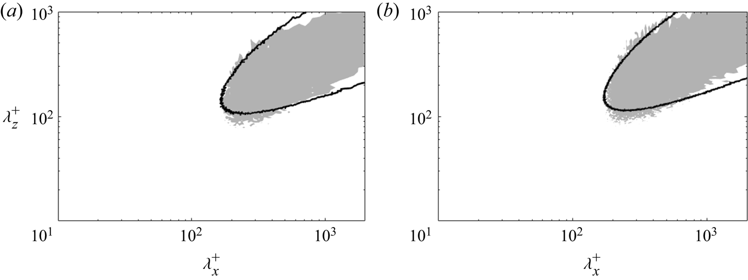
Figure 13. Two-dimensional pre-multiplied energy spectra  ${k_x}{k_z}{\varPhi _{uu}}$ (in shade) normalized by local intensity compared with the DNS (solid lines) (del Alamo et al. Reference del Alamo, Jimenez, Zandonade and Moser2004) at the outer location $y_{out}^ + \approx 3.9\sqrt {R{e_\tau }} $ at two Reynolds numbers: (a) $R{e_\tau } \approx 1000$; (b) $\; R{e_\tau } \approx 2000$. The contour levels are (a) 0.035 and (b) 0.025 of the local streamwise intensity.
Figure 14 shows the one-dimensional pre-multiplied energy spectra  ${k_z}{\varPhi _{uu}}$ as functions of spanwise wavelengths $\lambda _z^ + $ and wall distances ${y^ + }$. These results underscore the existence of two energy peaks predicted by the present WeDNS in comparison with the full DNS (Lee & Moser Reference Lee and Moser2015): the first inner one located at ${y^ + } \approx 13.5$ and the second outer one located in the log-law region, stretching from ${y^ + } \approx 3\sqrt {R{e_\tau }} $ to $y/\delta \approx 0.3$. The inner and outer energy peaks both can be observed in the present results (figure 14a). The inner region within the local embedded fine-mesh block is marked by the smaller black box. The first energy peak is with the dominant spanwise wavelength of $\lambda _z^ + \approx {10^2}$. The task to capture and resolve the first energy peak and near-wall small-scale dynamics is carried out in the fine-mesh embedded DNS block where the local solutions agree very well with the full DNS, as shown previously in figures 12(a) and 12(c). The second peak in the outer flow region contributed by the energetic large scales reaches a maximum beyond $y_s^ + = 3\sqrt {R{e_\tau }} $ that extends to the middle of the channel with the dominant spanwise wavelength of $\lambda _z^ + \approx O({10^3})$ (Agostini & Leschziner Reference Agostini and Leschziner2014) in wall units or ${\lambda _z} \approx \delta $ in the outer dimension. These large structures should be scaled with the outer variables and increase in wall units in y growing with Reynolds number. Note that the largest scales approaching the middle of the channel are cut off by the limited global domain size adopted in the present study. The influence of even larger scales is discussed by Lozano-Duran & Jimenez (Reference Lozano-Duran and Jimenez2014), which is beyond the scope of the present paper.
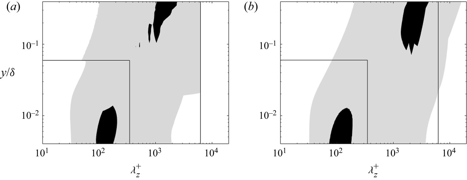
Figure 14. (a) One-dimensional pre-multiplied energy spectra  ${k_z}{\varPhi _{uu}}$ compared with (b) DNS (Lee & Moser Reference Lee and Moser2015) results at $R{e_\tau } \approx 2000$. The contour levels are 0.05/0.35 (of the local intensity). The inner smaller box marks the local embedded block, while the larger box marks the global full domain used in the present work.
5.3. ‘Foot-printing’ and ‘modulation’ in near-wall region
In this section, we will examine the instantaneous flow field in the near-wall region with an emphasis on the scale interdependence and interactions. The ‘foot-printing’ effect of the outer flow large structures on the near-wall flow motions will be examined by correlating the inner flow large scales to those of the outer flow. Furthermore, we will also analyse the interaction between the large coherent scales and small scales in a form of corresponding intermediate scales (‘modulation’) in the near-wall region.
The Huang–Hilbert empirical mode decomposition (EMD) method (Huang et al. Reference Huang, Shen, Long, Wu, Shih, Zheng, Yen, Tung and Liu1998) is applied to the instantaneous raw velocity field of the present WeDNS at  $R{e_\tau } \approx 2000$. The algorithm splits the original signals into a set of intrinsic mode functions (IMFs) based on local characteristic scales without introducing any cut-off wavelengths. This EMD method of a 2-D version is applied to decompose small- and large-scale components in DNS channel flows notably by Agostini & Leschziner (Reference Agostini and Leschziner2014, Reference Agostini and Leschziner2016a, Reference Agostini and Leschziner2016b, Reference Agostini and Leschziner2019). In the present work, with the implementation of the EMD code originally developed by Bhuiyan, Adhami & Khan (Reference Bhuiyan, Adhami and Khan2008), the last three of eight IMFs are retained as the long-pass filtered large-scale flow field. The raw data of instantaneous streamwise velocity fluctuations at an inner and outer location are shown in figures 15(a) and 15(b), respectively. The filtered large-scale structures of the inner field (figure 15c) show a clear resemblance to those of the outer flow when the local fine scales are filtered out (figure 15e). These filtered inner and outer fields are further compared by matching the zero-value contour lines of the outer flow (figure 15e) and the positive-value contours of the inner flow (figure 15c), which leads to the composite contour plot in figure 15(d). Note closely that the near-wall large scales travel continuously across the coarse–fine interface (figures 15c and 15d), similar to the contour lines cut across the interfaces smoothly seen previously in figure 8.
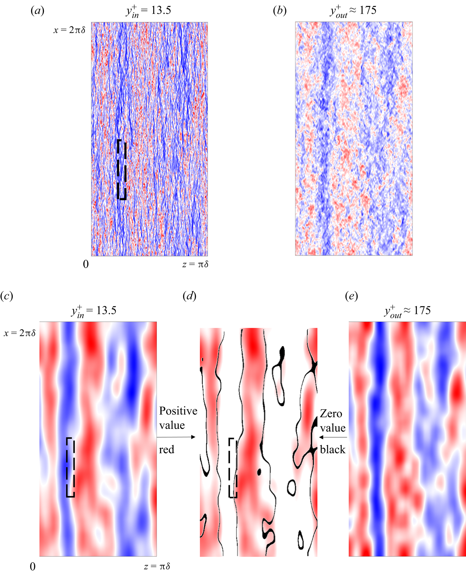
Figure 15. Illustration of the ‘foot-printing’ effect: (a) original inner instantaneous velocity field at location  $y_{in}^ +{=} 13.5$; (b) original instantaneous velocity field at $y_{out}^ +{\approx} 3.9\sqrt {R{e_\tau }} \approx 175$; (c) long-pass filtered field of panel (a); (d) red contours for the positive value of panel (c) while black lines sketch the zero envelop of panel (e); (e) long-pass filtered field of panel (b). In panel (d), the outer field snapshot is adjusted as per the inclination angle in y to be compared with the inner. All contours range from −3 (blue) to +3 (red) standard deviations of each field. Black dashed boxes indicate the embedded fine-mesh block.
Recognizing that the global coarse mesh for the whole domain under-resolves the disturbances when approaching the wall, we nevertheless can still observe clear correlations between inner and outer large-scale coherent structures. This is taken as the evidence of the ‘foot-printing’ of the outer scales on the inner region, which provides the signatures of the large scales of the global outer field on the locally embedded fine-mesh block.
Figure 16 is generated to illustrate the scale interactions between the large ‘footprints’ and the small local scales in the form of ‘modulation’ (Mathis et al. Reference Mathis, Hutchins and Marusic2009), manifested in the presence of some intermediate structures enveloped (conditioned) by the large structures of the outer flow. The inner small-scale fluctuations are retained in figure 16(b) by simply removing the large scales. This is enabled by subtracting the long-pass filtered field shown in figure 15(c) from the near-wall raw field in figure 16(a), similar to that performed by Marusic, Baars & Hutchins (Reference Marusic, Baars and Hutchins2017). We then apply the long-pass filter to the small-scale fluctuations and retain only the ‘positive’ islands shown in figure 16(c). The ‘footprinting’, as demonstrated in figure 15(d), is duplicated in figure 16(d). The presence of intermediate scales is clearly seen in figure 16(c).

Figure 16. Illustration of the ‘modulation’: (a) the original instantaneous velocity field at the inner location  $y_{in}^ +{=} 13.5$ (duplication of figure 15a); (b) equivalent short-pass filtered field of panel (a) (the raw field minus the filtered flow field in figure 15c); (c) long-pass filtered field of panel (b) with only contours of positive values retained, to be compared with the zero envelopes of panel (d); (d) duplication of figure 15(d) showing the large-scale ‘footprints’. All contours range from −3 (blue) to +3 (red) standard deviations of each field. Black dashed boxes indicate the local embedded fine-mesh domain.
The near-wall incoherent scales are the local ‘universal’ small scales modulated by the large-scale movement. We compare figure 16(c) and (d) more closely in a closeup of the embedded fine-mesh region in figure 17. The ‘modulation’ being the small-scales response to the large scales is seen to correlate to the near-wall large-scale structures, therefore is fused with the ‘footprints’. If we inspect the length-scale discrepancy of the near-wall coherent large scales (figure 16d) and the near-wall incoherent scales (figure 17a), we can easily observe that the former naturally is much larger than the size of the embedded block, while the latter is much smaller and well resolved by the local fine-mesh DNS. The ‘modulation’ due to the inter-scale interaction appears at the intermediate scales (figure 16c and figure 17b).
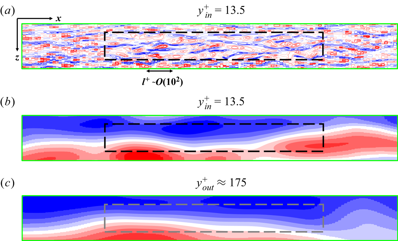
Figure 17. The instantaneous velocity fields at the vicinity of the embedded region as the green box in figure 16(b) enlarged: (a) local small-scale-pass filtered field near wall (close-up view of figure 16b); (b) intermediate scales indicative of the ‘modulation’ (close-up view of figure 16(c) with negative values added as shown in blue); (c) outer large-scale-pass filtered field (close-up view of figure 15e). The black dashed boxes in panels (a) and (b) mark the local embedded block. The grey dashed box in panel (c) only indicates the corresponding location of the embedded block underneath.
6. Wall-embedded LES
In this section, the potential applications of the two-scale approach are illustrated for WeLES cases at  $R{e_\tau } \approx 2000$, 4100 and 5200. The results are compared with the existing DNS database (Bernardini et al. Reference Bernardini, Pirozzoli and Orlandi2013; Lee & Moser Reference Lee and Moser2015). Once again, a given mass flow rate is targeted to match the same $R{e_b}$ as that of a full DNS. The mean velocity profiles predicted by the present WeLES are shown in figure 18(a–c), in good agreement with the corresponding DNS data for the three Reynolds numbers, respectively.

Figure 18. Mean velocity profiles at high Reynolds numbers: (a)  $R{e_\tau } \approx 2000$; (b) $R{e_\tau } \approx 4100$; (c) $R{e_\tau } \approx 5200$. The blue diamond symbols indicate results within the local fine-mesh block. The red squares and red solid lines indicate results in the global coarse outer and inner region, respectively. (d) Comparison in the mean velocity between the one-scale direct solution (‘One-scale5200’ shown as a dashed red line) and the present two-scale solutions (‘Two-scale5200’) with the source-term coupling on the same mesh grids at $R{e_\tau } \approx 5200$. Note that not all data points are included to increase readability.
The comparisons between the computed Reynolds number based on the friction velocity  $R{e_{\tau ,computed}}$ and those targeted $R{e_{\tau ,target}}$ are presented in table 4 indicating the accuracy in the wall shear-stress prediction. The cases computed by using the present two-scale method are labelled as ‘Two-scale2000’, ‘Two-scale4100’ and ‘Two-scale5200’ for the three nominal Reynolds numbers. Also included in the table are the two high-Reynolds-number (4100, 5200) cases computed without the source term coupling in the global inner region. These two computed cases without the source-term coupling are effectively single-scale direct solutions, thus are labelled as ‘One-scale4100’ and ‘One-scale5200’ for the two Reynolds numbers. The errors of the two-scale method solutions are all well within 1 % for these two high-Reynolds-number cases. In contrast, a much larger error (∼15 %) results from the near-wall coarse-mesh under-resolution when no source-term corrections are applied as in the direct one-scale solutions. The mean velocity profile in a closeup in the near-wall region predicted by the one-scale solution is compared with the two-scale and the DNS results, as shown in figure 18(d), in which the impact of the source term correction is clearly highlighted.
Table 4. Wall shear-stress prediction of the two-scale WeLES approach.
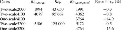
Extra attention is paid to the local fine-mesh block of the WeLES. Although this is an LES case, the local embedded block is assumed to be able to capture the inner energy peak comparably to a full DNS. The computed energy spectrum of the inner embedded block solution is shown in figure 19, which agrees well with the DNS.

Figure 19. (a) One-dimensional energy spectrum at  ${y^ + } = 13.5$ in relation to spanwise wavenumbers within the local fine-mesh block (blue diamonds) compared with the DNS results (black solid line, Lee & Moser Reference Lee and Moser2015) at $R{e_\tau } \approx 2000$. (b) One-dimensional premultiplied energy spectrum ${k_z}\varPhi _{uu}^ + $ in relation to wavelengths and wall distance in the inner region within the embedded block (greyscale contours) compared with the dashed contour lines for the DNS results from the database (Lee & Moser Reference Lee and Moser2015) at $R{e_\tau } \approx 2000$. The contour levels are 0.5/1.5/2.5.
Finally, figure 20 presents the estimated mesh-count scaling with Reynolds number compared with the actual mesh-count values adopted for the present WeLES computations. The two-scale approach with the locally embedded fine-mesh solution indicates a remarkable potential for computational efficiency gains.
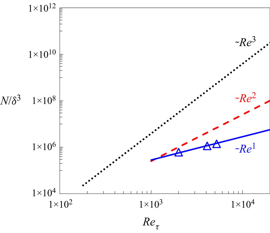
Figure 20. Comparison in mesh-count scaling with Reynolds number between the full WRLES (red dash lines) and the present two-scale WeLES (blue solid lines) underlined by the actual mesh counts of the present WeLES cases (blue triangles). The full DNS scaling (black dots) is also included.
7. Summary and conclusions
When seeking an efficient and accurate solution for wall-bounded turbulent flows by coupling a local near-wall fine-mesh block with a global coarse-mesh domain, we face two challenging issues: first, how to capture and resolve the distinctive influence of large-scale turbulent structures of the outer flow region on the near-wall turbulence, as clearly established and consistently substantiated in recent research findings, and second, how to correct the under-resolved global coarse-mesh near-wall region outside the local fine-mesh block.
We develop a two-scale method with a locally embedded fine-mesh block generated by sub-dividing the base coarse mesh cells in the near-wall region. The wall-normal height of the fine-mesh block is taken at the low bound of the log-law region (Marusic et al. Reference Marusic, Monty, Hultmark and Smits2013) and the streamwise and spanwise sizes are taken based on the spatial spectra of the full DNS data (Lee & Moser Reference Lee and Moser2015) to ensure sufficient coverage of the resolved ‘universal’ small-scale dynamics and the associated turbulence peak region for a wide range of Reynolds numbers. Correspondingly, the base coarse-mesh resolution in both the global outer flow and global near-wall regions is assumed to be sufficiently fine to capture and resolve all large-scale turbulence structures.
The influence of the large-scale structures on the locally embedded fine-mesh block is captured by a scale-dependent interface treatment with the distinctive and closely relevant capability, which is lacking in previous commonly adopted MFU-based methods. The coarse-mesh resolved disturbances can now be directly exchanged across a coarse–fine mesh domain interface, whilst only are the fine-mesh resolved fluctuations around the coarse-mesh variables subject to the periodic condition at the pairing boundaries of the fine-mesh block in the two wall-parallel directions. The results through scale filtering re-composition clearly indicate the ‘footprints’ of the outer flow large structures on the local embedded block, as well as the intermediate scales expected from the large–small scale interactions (‘modulation’) in the near-wall region. In this two-scale framework, we make no assumptions in relation to the need for the presence of a scale separation or spectral gap between the disturbances of the global coarse-mesh domain and those of the local fine-mesh block. The spatial energy spectra predicted by the present two-scale method exhibit a substantial range where the two spectra obtained from the two domains overlap smoothly. It is a manifestation of the wide and continuous range of the length scales of disturbances captured by the present two-scale coupled system. More importantly, as confirmed by a single-point temporal spectrum, the local fine-mesh domain is shown to be subject to a full range of length scales from the smallest scales resolved locally to the largest one dictated by the global domain size.
The global coarse-mesh in the near-wall region is under-resolved as expected. We resort to upscaling through a space–time averaging. The time-averaged and locally volume-averaged fine-mesh solution for corresponding coarse-mesh cells is taken as a target for the coarse-mesh region outside the embedded fine-mesh block. The corresponding forcing source terms, generated from the target solution of the fine-mesh block, are directly mapped to the corresponding coarse-mesh cells in the global inner domain, given the homogeneity of the time-averaged field in the streamwise and spanwise directions. With the pointwise source terms-based corrections, the coupling between the two domains directly reflects the physical interaction: the global domain provides improved conditioning for the local embedded fine-mesh block whilst the local fine-mesh block solution provides means to lead to an effectively improved resolution for the global domain. It follows that the improved near-wall solutions of both the embedded fine-mesh block and the coarse-mesh inner region in turn lead to improved conditioning for the global outer flow region.
The two-scale method is examined for an incompressible channel flow. Validation case studies are carried for  $R{e_\tau } \approx 550$, 1000 and 2000, with the mean statistics and energy spectra being compared with the corresponding full DNS data (del Alamo et al. Reference del Alamo, Jimenez, Zandonade and Moser2004; Lee & Moser Reference Lee and Moser2015). Analyses using the Huang–Hilbert EMD method for scale decomposition and re-composition, in a similar way to that of Marusic et al. (Reference Marusic, Baars and Hutchins2017), clearly illustrate the ‘foot-printing’ and the ‘modulation’ effects in the local fine-mesh block. It is shown that the mesh-count scaling with Reynolds number can be potentially reduced from $O(R{e^2})$ for conventional wall-resolved large-eddy simulations (WRLES) to $O(Re)$ for the present local wall-embedded LES (WeLES). Further LES tests are conducted for $R{e_\tau } \approx 2000$, 4100 and 5200, which demonstrate the projected mesh count gains and the improved accuracy of the present method over a direct coarse-mesh solution without the two-scale source-term coupling.
Finally, some further comments should be made regarding the prospect of applying the present two-scale methodology as described to more practical applications. The seemingly restrictive feature of a channel flow is the homogeneity of the time-averaged flow in the two wall-parallel directions. We intentionally make use of the simple canonical configuration to highlight the most relevant while generally applicable key difference between an unsteady field and its time-averaged counterpart. The latter is much smoother than the former, thus a source term correction based on a time-invariant averaged (instead of an instantaneous) flow would be far more readily amenable to spectral mapping efficiently and accurately in the two wall-parallel directions for wall-bounded turbulence. This should be the case for many practical wall-bounded turbulence flows where a time-averaged flow is smooth while being inhomogeneous in two wall-parallel directions. As indicated in the introduction, the present work stems from a two-scale block spectral method development aimed at more specific practical problems, such as surface micro-structures, micro/effusion-cooling (He Reference He2018; Kapsis et al. Reference Kapsis, He, Li, Valero, Wells, Krishnababu, Gupta, Kapat and Schaenzer2020) and aerothermal analyses of multiple blade passages and rows (He Reference He2021), commonly subject to non-uniform flow conditions and geometries. The work presented in this paper should provide a more fundamental while generalizable underpinning of the two-scale methodology, as motivated. Further developments and applications are expected.
Acknowledgements
The work is supported in part by the EU Horizon 2020 grant, Marie Skłodowska-Curie Actions (Control of Turbulence Fricion Force, CTFF). C.C. is on a scholarship from the China Scholarship Council (CSC). The authors would also like to acknowledge the use of the University of Oxford Advanced Research Computing (ARC).
Funding
EU Horizon 2020 grant, Marie Skłodowska-Curie Actions (H202-MSCA-2017, 777717, Control of Turbulence Fricion Force, CTFF).
Declaration of interests
The authors report no conflicts of interest.
Author contributions
C. Chen carried out the method implementation, case study set-up, simulations and data processing. L. He instigated the framework methodology and case study design. Both authors contributed equally to analysing and interpreting results, and in writing the paper.
Appendix A. An option for additional buffer layer
For the baseline implementation of the two-scale method, it is assumed that the ‘modulation’ can be mostly regarded as a one-way influence of the large scales in the outer flow region on the small scales and some intermediate scales in the near-wall region, as indicated in figure 17. However, the modulated near-wall turbulent flow should, in principle, be able to provide feedback to affect the outer large scales, which is neglected in the baseline implementation. Although the authors have so far not seen any noticeable feedback effects, the issue should be dealt with for completeness of the framework and implementation method. In this Appendix, we consider a very simple option without extra mesh-cost to include this feedback, should it become significant.
As illustrated in figure 21, we take a local region of the coarse-mesh domain directly adjacent to the embedded fine-mesh block as a target buffer region (labelled as ‘Buffer 1’). Correspondingly, we take a global buffer region to be corrected which is adjacent to the global inner coarse-mesh region, labelled as ‘Buffer 2’. A phenomenological argument within the two-scale framework follows that if the ‘modulation’ resolved in the near-wall fine-mesh block does have non-negligible feedback on the outer flow region, the buffer region adjacent to the local fine-mesh block will have to be different from that of the global outer coarse-mesh region directly adjacent to the coarse-mesh inner region. Thus, the time-averaged flow of Buffer 1 will have to be different from that of Buffer 2. As such, we can use the time-averaged flow of Buffer 1 as the target to correct Buffer 2.
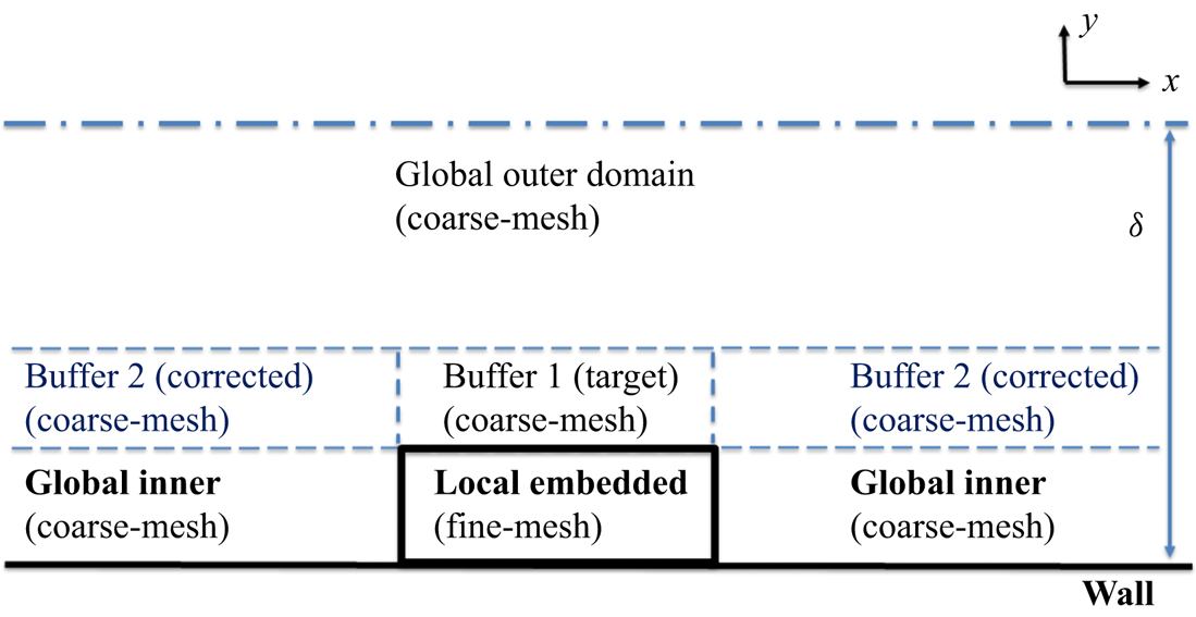
Figure 21. Domain with coarse-mesh buffer regions (an extended version of figure 1b).
For the buffer regions, the general upscaled coarse-mesh flow equations (3.12) can be written as
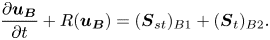 \begin{equation}\frac{{\partial {\boldsymbol{u}_{\boldsymbol{B}}}}}{{\partial t}} + R({\boldsymbol{u}_{\boldsymbol{B}}}) = {({\boldsymbol{S}_{st}})_{B1}} + {({\boldsymbol{S}_t})_{B2}}.\end{equation}
For the target region Buffer 1, the space–time averaging is now reduced to time averaging only. Thus, the driving source is simply generated taking the inverse mode of the time averaging:
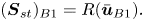 \begin{equation}{({\boldsymbol{S}_{st}})_{B1}} = R({\bar{\boldsymbol{u}}_{B1}}).\end{equation}
For Buffer 2, making use of (3.15), we have the upscaled equation:
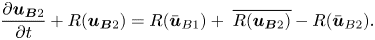 \begin{equation}\frac{{\partial {\boldsymbol{u}_{\boldsymbol{B}2}}}}{{\partial t}} + R({\boldsymbol{u}_{\boldsymbol{B}2}}) = R({\bar{\boldsymbol{u}}_{B1}}) + \; \overline {R({\boldsymbol{u}_{\boldsymbol{B}2}})} - R({\bar{\boldsymbol{u}}_{B2}}).\end{equation}
After time averaging equation (A3), we then get the resultant equation driving the converged time-averaged flow in Buffer 2 to the target in Buffer 1, as intended:
 \begin{equation}R({\bar{\boldsymbol{u}}_{B2}}) = \; R({\bar{\boldsymbol{u}}_{B1}}). \end{equation}
It is emphasized that the implementation of this option does not involve any extra mesh, as all the buffer regions are of the coarse mesh which is meant to be sufficiently fine to resolve all relevant scales locally. The only extra cost will be that for local time averaging, and that for evaluating and actuating the time-averaging source terms in the inverse or the direct mode for the two buffer regions, which tend to be minimally small.
The two-scale method with the added extra buffer regions is tested for the case with  $R{e_\tau } \approx 5200$ in which the buffer thickness is taken to be $0.05\delta $. The comparison between the results with and without the buffer shows negligible differences for the case tested. This further test would suggest that for the present cases at the given Reynolds numbers, the ‘modulation’ can still be regarded as predominantly only influential on small and intermediate scales in the near-wall region without noticeable feedback to the large scales themselves in the outer flow region.


 Open access