


1 Introduction
The role of surface roughness in boundary layer transition is significant due to its impact in aerodynamic and aero-thermodynamic problems. Typically, the effect of roughness elements in promoting boundary layer transition is estimated by the roughness-height-based Reynolds number, defined as $Re_{h}=u_{h}h/\unicode[STIX]{x1D708}$
, where
$Re_{h}=u_{h}h/\unicode[STIX]{x1D708}$
, where $h$
is the roughness height and
$h$
is the roughness height and $u_{h}$
is the streamwise velocity at that height (van Driest & McCauley Reference van Driest and Mccauley1960; Tani Reference Tani1969). For a two-dimensional roughness element without spanwise variation (e.g. step, gap or ribbon), the natural transition process is promoted by amplification of Tollmien–Schlichting (TS) waves at the downstream separation and recovery region of the roughness (Klebanoff & Tidstrom Reference Klebanoff and Tidstrom1972). Increasing
$u_{h}$
is the streamwise velocity at that height (van Driest & McCauley Reference van Driest and Mccauley1960; Tani Reference Tani1969). For a two-dimensional roughness element without spanwise variation (e.g. step, gap or ribbon), the natural transition process is promoted by amplification of Tollmien–Schlichting (TS) waves at the downstream separation and recovery region of the roughness (Klebanoff & Tidstrom Reference Klebanoff and Tidstrom1972). Increasing $Re_{h}$
leads to the growth of TS wave amplitude (Saric, Reed & Kerschen Reference Saric, Reed and Kerschen2002), thus moving the transition location gradually upstream, closer to the roughness element (Perraud et al.
Reference Perraud, Arnal, Seraudie and Tran2004). For three-dimensional distributed or isolated roughness, the transition process cannot be explained by the enhancement of TS waves, as three-dimensional roughness introduces a localized spanwise deflection of the streamlines without strong downstream flow separation. The wake flow of three-dimensional roughness features the generation of counter-rotating streamwise vortex pairs (Joslin & Grosch Reference Joslin and Grosch1995; Fransson et al.
Reference Fransson, Brandt, Talamelli and Cossu2004). The streamwise vortices induce an upwash motion on one side, transporting low momentum fluid away from the wall, and on the other side, they sweep high momentum fluid towards the wall, resulting in the formation of low- and high-speed streaks which modulate the surface shear along the spanwise direction. Similarly, in the bypass transition process, the formation of velocity streaks through the lift-up mechanism takes over the role of TS waves in the process of the growth of the perturbations (Landahl Reference Landahl1990). Once the streak amplitude exceeds a critical value, the streak will be subject to a secondary instability, with either sinuous or varicose modulation, and finally breaks down into turbulence (Andersson et al.
Reference Andersson, Brandt, Bottaro and Henningson2001).
$Re_{h}$
leads to the growth of TS wave amplitude (Saric, Reed & Kerschen Reference Saric, Reed and Kerschen2002), thus moving the transition location gradually upstream, closer to the roughness element (Perraud et al.
Reference Perraud, Arnal, Seraudie and Tran2004). For three-dimensional distributed or isolated roughness, the transition process cannot be explained by the enhancement of TS waves, as three-dimensional roughness introduces a localized spanwise deflection of the streamlines without strong downstream flow separation. The wake flow of three-dimensional roughness features the generation of counter-rotating streamwise vortex pairs (Joslin & Grosch Reference Joslin and Grosch1995; Fransson et al.
Reference Fransson, Brandt, Talamelli and Cossu2004). The streamwise vortices induce an upwash motion on one side, transporting low momentum fluid away from the wall, and on the other side, they sweep high momentum fluid towards the wall, resulting in the formation of low- and high-speed streaks which modulate the surface shear along the spanwise direction. Similarly, in the bypass transition process, the formation of velocity streaks through the lift-up mechanism takes over the role of TS waves in the process of the growth of the perturbations (Landahl Reference Landahl1990). Once the streak amplitude exceeds a critical value, the streak will be subject to a secondary instability, with either sinuous or varicose modulation, and finally breaks down into turbulence (Andersson et al.
Reference Andersson, Brandt, Bottaro and Henningson2001).
The conditions at which transition is induced by three-dimensional roughness are typically characterized by a critical $Re_{h}$
. The value of this is obtained by experiments (Tani et al.
Reference Tani, Komoda, Komatsu and Iuchi1962) and is defined as the value where transition begins to depend upon the presence of the roughness element, compared to the smooth wall condition (van Driest & McCauley Reference van Driest and Mccauley1960). Below the critical
$Re_{h}$
. The value of this is obtained by experiments (Tani et al.
Reference Tani, Komoda, Komatsu and Iuchi1962) and is defined as the value where transition begins to depend upon the presence of the roughness element, compared to the smooth wall condition (van Driest & McCauley Reference van Driest and Mccauley1960). Below the critical $Re_{h}$
, the transition location is not affected by the roughness element. The flow in the wake of the roughness element remains stable and returns to homogeneous laminar conditions after a certain distance. Instead, when exceeding the threshold, transition will rapidly move upstream (with increasing Reynolds number) until it coincides with the roughness location. Klebanoff, Schubauerand & Tidstrom (Reference Klebanoff, Schubauerand and Tidstrom1955) proposed an empirical estimate of the critical
$Re_{h}$
, the transition location is not affected by the roughness element. The flow in the wake of the roughness element remains stable and returns to homogeneous laminar conditions after a certain distance. Instead, when exceeding the threshold, transition will rapidly move upstream (with increasing Reynolds number) until it coincides with the roughness location. Klebanoff, Schubauerand & Tidstrom (Reference Klebanoff, Schubauerand and Tidstrom1955) proposed an empirical estimate of the critical $Re_{h}$
for three-dimensional isolated roughness with aspect ratio (
$Re_{h}$
for three-dimensional isolated roughness with aspect ratio ( $h/c$
) of unity, lying in the range between 600 and 900 for incompressible flows based on existing experimental results. Later, von Doenhoff & Braslow (Reference von Doenhoff, Braslow and Lachmann1961) obtained a correlation between the critical
$h/c$
) of unity, lying in the range between 600 and 900 for incompressible flows based on existing experimental results. Later, von Doenhoff & Braslow (Reference von Doenhoff, Braslow and Lachmann1961) obtained a correlation between the critical $Re_{h}$
and the aspect ratio of roughness element, scaling with
$Re_{h}$
and the aspect ratio of roughness element, scaling with $(h/c)^{2/5}$
. Although providing a basic guideline for the prediction of forced transition, the critical Reynolds number
$(h/c)^{2/5}$
. Although providing a basic guideline for the prediction of forced transition, the critical Reynolds number $Re_{h,crit}$
does not give insight into the physical mechanism and is still influenced by many factors, such as roughness shape and free stream disturbance level, questioning the generality of the proposed value (Reda Reference Reda2002).
$Re_{h,crit}$
does not give insight into the physical mechanism and is still influenced by many factors, such as roughness shape and free stream disturbance level, questioning the generality of the proposed value (Reda Reference Reda2002).
The value of $Re_{h}$
has an important effect on the streak amplitude, length scales and perturbation growth rate (Choudhari & Fischer Reference Choudhari and Fischer2005; Ergin & White Reference Ergin and White2006; Denissen & White Reference Denissen and White2008). The former factors can modulate the route towards transition. Ergin & White (Reference Ergin and White2006) studied the transitional flow over a spanwise array of cylinder-shaped roughness by using hot-wire anemometry at various values of
$Re_{h}$
has an important effect on the streak amplitude, length scales and perturbation growth rate (Choudhari & Fischer Reference Choudhari and Fischer2005; Ergin & White Reference Ergin and White2006; Denissen & White Reference Denissen and White2008). The former factors can modulate the route towards transition. Ergin & White (Reference Ergin and White2006) studied the transitional flow over a spanwise array of cylinder-shaped roughness by using hot-wire anemometry at various values of $Re_{h}$
, ranging from subcritical (
$Re_{h}$
, ranging from subcritical ( $Re_{h}=202$
and 264) to supercritical conditions (
$Re_{h}=202$
and 264) to supercritical conditions ( $Re_{h}=334$
). For all
$Re_{h}=334$
). For all $Re_{h}$
studied, the presence of high velocity fluctuations located at the inflection point of the velocity profile indicates a possible effect of Kelvin–Helmholtz (K–H) instability on transition. They also found the exponential growth rate of the unsteady disturbances increases rapidly with increasing
$Re_{h}$
studied, the presence of high velocity fluctuations located at the inflection point of the velocity profile indicates a possible effect of Kelvin–Helmholtz (K–H) instability on transition. They also found the exponential growth rate of the unsteady disturbances increases rapidly with increasing $Re_{h}$
. At supercritical
$Re_{h}$
. At supercritical $Re_{h}$
, the unsteady disturbances undergo transient growth and spread laterally across the wake, leading to transition to turbulence. At subcritical conditions, the unsteady disturbances are damped before transition can occur, returning a Blasius condition. Using direct numerical simulation (DNS), Rizzetta & Visbal (Reference Rizzetta and Visbal2007) analysed the flow past cylinder arrays for the same values of
$Re_{h}$
, the unsteady disturbances undergo transient growth and spread laterally across the wake, leading to transition to turbulence. At subcritical conditions, the unsteady disturbances are damped before transition can occur, returning a Blasius condition. Using direct numerical simulation (DNS), Rizzetta & Visbal (Reference Rizzetta and Visbal2007) analysed the flow past cylinder arrays for the same values of $Re_{h}$
as the experiment of Ergin & White (Reference Ergin and White2006). Bypass transition was found at supercritical
$Re_{h}$
as the experiment of Ergin & White (Reference Ergin and White2006). Bypass transition was found at supercritical $Re_{h}=334$
. The transition process is strongly influenced by hairpin vortex structure. At subcritical
$Re_{h}=334$
. The transition process is strongly influenced by hairpin vortex structure. At subcritical $Re_{h}$
, low amplitude disturbances are generated in the cylinder wake, undergoing exponential growth. Different from the experimental result, transition also appears at the downstream extent of the computation domain.
$Re_{h}$
, low amplitude disturbances are generated in the cylinder wake, undergoing exponential growth. Different from the experimental result, transition also appears at the downstream extent of the computation domain.
In order to understand the instability mechanism behind roughness elements, Cherubini et al. (Reference Cherubini, de Tullio, de Palma and Pascazio2013) searched for the perturbations inducing the largest disturbance energy growth in the wake of a three-dimensional smooth bump by performing linear optimization analysis. The mean flow field shows streamwise velocity streaks. Two optimal disturbance shapes were found for large roughness, being described as varicose perturbations related to K–H instability, and sinuous perturbations located at the lateral shear layer. The definition of the instability modes is based on the symmetric and asymmetric appearance of the streamwise velocity perturbations. The varicose mode can lead to faster energy growth compared with the sinuous mode at $Re_{h}$
close to the critical value. The unit Reynolds number based on free stream velocity has a stronger effect on the structure of optimal disturbances than
$Re_{h}$
close to the critical value. The unit Reynolds number based on free stream velocity has a stronger effect on the structure of optimal disturbances than $Re_{h}$
. Nevertheless, increasing both parameters leads to a fast growth of the perturbations, causing early transition. In the recent DNS study performed by Loiseau et al. (Reference Loiseau, Robinet, Cherubini and Leriche2014), velocity streaks were also observed in the wake of discrete cylinders. Increasing
$Re_{h}$
. Nevertheless, increasing both parameters leads to a fast growth of the perturbations, causing early transition. In the recent DNS study performed by Loiseau et al. (Reference Loiseau, Robinet, Cherubini and Leriche2014), velocity streaks were also observed in the wake of discrete cylinders. Increasing $Re_{h}$
from a subcritical to supercritical value results in a longer streamwise persistence of a low-speed region around the symmetry plane. The result of a three-dimensional global stability analysis indicates that both the varicose and sinuous modes can be produced in the roughness wake. The dominance of the instability mode type on transition strongly depends on the Reynolds number and aspect ratio of the roughness element.
$Re_{h}$
from a subcritical to supercritical value results in a longer streamwise persistence of a low-speed region around the symmetry plane. The result of a three-dimensional global stability analysis indicates that both the varicose and sinuous modes can be produced in the roughness wake. The dominance of the instability mode type on transition strongly depends on the Reynolds number and aspect ratio of the roughness element.
Despite the intensive research on the effect of Reynolds number on roughness-induced transition, most attention has been paid to the statistical analyses of perturbation growth and modal analysis in incompressible flows. Detailed analysis of the instantaneous flow organization dependence on the Reynolds number is necessary to consolidate the understanding of transition process. Ye, Schrijer & Scarano (Reference Ye, Schrijer and Scarano2016a
,Reference Ye, Schrijer and Scarano
b
) measured the three-dimensional vortical structures in the wake of isolated roughness elements having different geometries (cylinder, square, hemisphere and micro-ramp) at supercritical $Re_{h}$
using tomographic particle image velocimetry (PIV). The mean flow pattern was well captured, featuring a system of multiple counter-rotating vortex pairs in the near wake region. The instantaneous flow organization reveals the onset of hairpin vortices, following different evolution processes towards transition in the wake of various elements. As the former study only dealt with the supercritical condition, the unsteady flow behaviour closer to critical
$Re_{h}$
using tomographic particle image velocimetry (PIV). The mean flow pattern was well captured, featuring a system of multiple counter-rotating vortex pairs in the near wake region. The instantaneous flow organization reveals the onset of hairpin vortices, following different evolution processes towards transition in the wake of various elements. As the former study only dealt with the supercritical condition, the unsteady flow behaviour closer to critical $Re_{h}$
needs to be explored. Furthermore, it is particularly desired to identify the vortical structures that may contribute to the instability mechanism, leading to the interest in applying proper orthogonal decomposition (POD), which is an efficient tool for data reduction in the field of fluid mechanics (Lumley Reference Lumley, Yaglom and Tatarski1967). The obtained eigenmodes can shed light on the dominant flow features and their relation with the instability modes and can facilitate a reduced-order description of the flow field.
$Re_{h}$
needs to be explored. Furthermore, it is particularly desired to identify the vortical structures that may contribute to the instability mechanism, leading to the interest in applying proper orthogonal decomposition (POD), which is an efficient tool for data reduction in the field of fluid mechanics (Lumley Reference Lumley, Yaglom and Tatarski1967). The obtained eigenmodes can shed light on the dominant flow features and their relation with the instability modes and can facilitate a reduced-order description of the flow field.
Most previous studies have focused on the bluff-front roughness elements (cylinder, square and sphere), which produce horseshoe vortices by upstream flow separation (Baker Reference Baker1979). Less effort has been spent on slender-shaped roughness elements, such as the micro-ramp, which will introduce a mild modulation of the mean flow, thus requiring much longer distance for the onset of transition (Ye et al. Reference Ye, Schrijer and Scarano2016a ). The micro-ramp geometry has been widely used as a flow control device to enhance boundary layer mixing, promote transition and avoid unwanted separation (Berry et al. Reference Berry, Auslender, Dilley and Calleja2001; Lin Reference Lin2002). In the special case of shock wave boundary layer interactions (SWBLI) with an incoming supersonic turbulent boundary layer, the micro-ramp has also gained substantial research attention due to its effectiveness in reducing separation (Dolling Reference Dolling2001; Babinsky, Li & PittFord Reference Babinsky, Li and Pittford2009; Giepman, Schrijer & van Oudheusden Reference Giepman, Schrijer and van Oudheusden2014).
The present investigation employs tomographic PIV to capture the three-dimensional aspects of the evolution towards transition in the wake behind a micro-ramp. The experiments are conducted covering the range from supercritical to subcritical $Re_{h}$
(§ 2). The system of streamwise vortices and the induced velocity distribution is identified in the time-averaged flow topology (§ 3). The influence of
$Re_{h}$
(§ 2). The system of streamwise vortices and the induced velocity distribution is identified in the time-averaged flow topology (§ 3). The influence of $Re_{h}$
on the instantaneous flow organization is visualized by the iso-surface of
$Re_{h}$
on the instantaneous flow organization is visualized by the iso-surface of $\unicode[STIX]{x1D706}_{2}$
criterion and the non-dimensional streamwise vorticity (§ 4). The full article corroborates the analysis with a statistical characterization of the velocity fluctuations (§ 5). The POD analysis (§ 6) returns the most energetic spatial modes, which are later identified as symmetric and asymmetric components of the growing velocity fluctuations. The low-order model consisting of selected POD modes highlights the development of secondary vortex structures, giving rise to the spanwise spreading of perturbations.
$\unicode[STIX]{x1D706}_{2}$
criterion and the non-dimensional streamwise vorticity (§ 4). The full article corroborates the analysis with a statistical characterization of the velocity fluctuations (§ 5). The POD analysis (§ 6) returns the most energetic spatial modes, which are later identified as symmetric and asymmetric components of the growing velocity fluctuations. The low-order model consisting of selected POD modes highlights the development of secondary vortex structures, giving rise to the spanwise spreading of perturbations.
2 Experiment set-up and data reduction
2.1 Wind tunnel, flow conditions and micro-ramp geometry
The experiments were conducted in the open jet low-speed wind tunnel at the Aerodynamic Laboratories of Delft University of Technology. The wind tunnel has an exit of $0.4\times 0.4~\text{m}^{2}$
following a contraction ratio of
$0.4\times 0.4~\text{m}^{2}$
following a contraction ratio of $9:1$
. An aluminium flat plate with a length of 700 mm, width of 400 mm and a thickness of 10 mm is placed at the mid-plane of the test section. A micro-ramp with 2 mm height (
$9:1$
. An aluminium flat plate with a length of 700 mm, width of 400 mm and a thickness of 10 mm is placed at the mid-plane of the test section. A micro-ramp with 2 mm height ( $h$
) and 4 mm span (
$h$
) and 4 mm span ( $c$
) is placed on the centreline at 290 mm downstream of the plate leading edge. The length (
$c$
) is placed on the centreline at 290 mm downstream of the plate leading edge. The length ( $l$
) of the micro-ramp is 4.5 mm, resulting in an incidence angle and half-sweep angle of
$l$
) of the micro-ramp is 4.5 mm, resulting in an incidence angle and half-sweep angle of $24^{\circ }$
, as shown in figure 1. The
$24^{\circ }$
, as shown in figure 1. The $x,y,z$
axes of the coordinate system correspond to the streamwise, wall-normal and spanwise directions respectively. The origin of the coordinate axis (
$x,y,z$
axes of the coordinate system correspond to the streamwise, wall-normal and spanwise directions respectively. The origin of the coordinate axis ( $o$
) is located in the symmetry plane at the wall, at the half-way point of the micro-ramp chord.
$o$
) is located in the symmetry plane at the wall, at the half-way point of the micro-ramp chord.

Figure 1. Micro-ramp geometry and coordinate definition, top, side and perspective view.
The experiments are carried out at free stream velocities ( $u_{\infty }$
) of 10, 7, 5 and
$u_{\infty }$
) of 10, 7, 5 and $4~\text{m}~\text{s}^{-1}$
. The corresponding ramp-height-based Reynolds numbers
$4~\text{m}~\text{s}^{-1}$
. The corresponding ramp-height-based Reynolds numbers $Re_{h}$
are 1170, 730, 460 and 320, respectively. The
$Re_{h}$
are 1170, 730, 460 and 320, respectively. The $Re_{h}$
values tested in the experiment are compared with the transition diagram provided by von Doenhoff & Braslow (Reference von Doenhoff, Braslow and Lachmann1961), as shown in figure 2. The grey area indicates the conditions where the growth of disturbances or transition may occur downstream of the roughness element, close to the critical case. When
$Re_{h}$
values tested in the experiment are compared with the transition diagram provided by von Doenhoff & Braslow (Reference von Doenhoff, Braslow and Lachmann1961), as shown in figure 2. The grey area indicates the conditions where the growth of disturbances or transition may occur downstream of the roughness element, close to the critical case. When $Re_{h}$
for a given value of
$Re_{h}$
for a given value of $c/h$
is below the grey area, the flow remains laminar downstream of the roughness element. If it is located above, transition is expected just downstream of the roughness element. Based on the roughness aspect ratio
$c/h$
is below the grey area, the flow remains laminar downstream of the roughness element. If it is located above, transition is expected just downstream of the roughness element. Based on the roughness aspect ratio $c/h$
of 2, the critical
$c/h$
of 2, the critical $Re_{h}$
of the experiments reported herein falls in the range between 320 to 460.
$Re_{h}$
of the experiments reported herein falls in the range between 320 to 460.
Figure 2. Comparison between current experimental conditions and the transition diagram provided by von Doenhoff & Braslow (Reference von Doenhoff, Braslow and Lachmann1961).
The undisturbed laminar boundary layer thickness ( $\unicode[STIX]{x1D6FF}_{99}$
) (without the roughness element) at the micro-ramp location is measured to be 3.26, 3.88, 4.52 and 5.30 mm for the different values of the free stream velocity respectively. The resulting ratio between roughness height and boundary layer thickness is
$\unicode[STIX]{x1D6FF}_{99}$
) (without the roughness element) at the micro-ramp location is measured to be 3.26, 3.88, 4.52 and 5.30 mm for the different values of the free stream velocity respectively. The resulting ratio between roughness height and boundary layer thickness is $h/\unicode[STIX]{x1D6FF}_{99}=0.61,0.52,0.44$
and 0.38. The properties of the undisturbed boundary layer, including displacement thickness (
$h/\unicode[STIX]{x1D6FF}_{99}=0.61,0.52,0.44$
and 0.38. The properties of the undisturbed boundary layer, including displacement thickness ( $\unicode[STIX]{x1D6FF}^{\ast }$
), momentum thickness (
$\unicode[STIX]{x1D6FF}^{\ast }$
), momentum thickness ( $\unicode[STIX]{x1D703}$
),
$\unicode[STIX]{x1D703}$
), $Re_{x}=u_{\infty }x/\unicode[STIX]{x1D708}$
and
$Re_{x}=u_{\infty }x/\unicode[STIX]{x1D708}$
and $Re_{\unicode[STIX]{x1D703}}=u_{\infty }\unicode[STIX]{x1D703}/\unicode[STIX]{x1D708}$
, are summarized in table 1. The shape factor reveals a relative constant value of
$Re_{\unicode[STIX]{x1D703}}=u_{\infty }\unicode[STIX]{x1D703}/\unicode[STIX]{x1D708}$
, are summarized in table 1. The shape factor reveals a relative constant value of $2.59\pm 0.05$
, indicating that the boundary layer remains laminar. The development of the undisturbed boundary layer profile on the flat plate is measured and compared with the theoretical solution based on Blasius self-similarity, yielding a good agreement until the most downstream region of the measurement domain. The detailed comparison can be retrieved from Ye et al. (Reference Ye, Schrijer and Scarano2016b
).
$2.59\pm 0.05$
, indicating that the boundary layer remains laminar. The development of the undisturbed boundary layer profile on the flat plate is measured and compared with the theoretical solution based on Blasius self-similarity, yielding a good agreement until the most downstream region of the measurement domain. The detailed comparison can be retrieved from Ye et al. (Reference Ye, Schrijer and Scarano2016b
).
Figure 3. Sketch of the experimental set-up including illumination and imaging system.
Table 1. Incoming flow conditions.

2.2 Tomographic PIV
The tomographic PIV system features four LaVision Imager Pro LX interline CCD cameras ( $4872\times 3248$
pixels,
$4872\times 3248$
pixels, $7.4~\unicode[STIX]{x03BC}\text{m}~\text{pixel}^{-1}$
) arranged along an arc with a maximum aperture angle of
$7.4~\unicode[STIX]{x03BC}\text{m}~\text{pixel}^{-1}$
) arranged along an arc with a maximum aperture angle of $\unicode[STIX]{x1D6FD}_{aperture}=60^{\circ }$
to obtain a good reconstruction accuracy, as shown in figure 3. The cameras were equipped with objectives of 105 mm focal length, which were tilted to comply with the Scheimpflug condition. The aperture was set at
$\unicode[STIX]{x1D6FD}_{aperture}=60^{\circ }$
to obtain a good reconstruction accuracy, as shown in figure 3. The cameras were equipped with objectives of 105 mm focal length, which were tilted to comply with the Scheimpflug condition. The aperture was set at $f_{\#}=11$
, resulting in a focal depth of 8.4 mm. The flow was seeded with a SAFEX fog machine that generates water–glycol droplets of approximately
$f_{\#}=11$
, resulting in a focal depth of 8.4 mm. The flow was seeded with a SAFEX fog machine that generates water–glycol droplets of approximately $1~\unicode[STIX]{x03BC}\text{m}$
diameter. The seeding concentration was carefully adjusted to approximately 4 particles mm
$1~\unicode[STIX]{x03BC}\text{m}$
diameter. The seeding concentration was carefully adjusted to approximately 4 particles mm $^{-3}$
. The measurement region was illuminated with a Quantel CFR PIV-200 Nd:YAG laser (
$^{-3}$
. The measurement region was illuminated with a Quantel CFR PIV-200 Nd:YAG laser ( $200~\text{mJ}~\text{pulse}^{-1}$
, 532 nm wavelength, 9 ns pulse duration). The pulse separation time was set to 30, 43, 60 and
$200~\text{mJ}~\text{pulse}^{-1}$
, 532 nm wavelength, 9 ns pulse duration). The pulse separation time was set to 30, 43, 60 and $75~\unicode[STIX]{x03BC}\text{s}$
, yielding a particle displacement of 10 pixels in the free stream for all flow conditions. The region of interest of the camera was cropped in the vertical direction resulting in an active sensor size of
$75~\unicode[STIX]{x03BC}\text{s}$
, yielding a particle displacement of 10 pixels in the free stream for all flow conditions. The region of interest of the camera was cropped in the vertical direction resulting in an active sensor size of $4872\times 1500$
pixels. The corresponding measurement volume size is
$4872\times 1500$
pixels. The corresponding measurement volume size is $145(x)\times 6(y)\times 45(z)~\text{mm}^{3}$
(
$145(x)\times 6(y)\times 45(z)~\text{mm}^{3}$
( $72.5h\times 3h\times 22.5h$
), resulting in a digital image resolution of
$72.5h\times 3h\times 22.5h$
), resulting in a digital image resolution of $33.6~\text{pixel}~\text{mm}^{-1}$
. The measurement domain begins from 5 mm behind the roughness centre and extends till 150 mm downstream. The wall-normal depth of the domain covers three ramp heights. The datasets consist of 200 snapshots for
$33.6~\text{pixel}~\text{mm}^{-1}$
. The measurement domain begins from 5 mm behind the roughness centre and extends till 150 mm downstream. The wall-normal depth of the domain covers three ramp heights. The datasets consist of 200 snapshots for $Re_{h}=1170$
, 730 and 460 and 50 snapshots for
$Re_{h}=1170$
, 730 and 460 and 50 snapshots for $Re_{h}=320$
, acquired at a frequency of 1.5 Hz.
$Re_{h}=320$
, acquired at a frequency of 1.5 Hz.
LaVision Davis 8 was used for system synchronization, calibration, data acquisition and processing. The three-dimensional relation between object and image space was obtained by physical calibration procedure using a custom-made calibration target. Further corrections reducing misalignment errors to below 0.1 pixels were obtained using three-dimensional (3-D) self-calibration (Wieneke Reference Wieneke2008). The raw images were pre-processed by the subtraction of the pixel time minimum and of the spatial minimum from a kernel of $31\times 31$
pixels. Image intensity was homogenized by normalization against the local average over a kernel of
$31\times 31$
pixels. Image intensity was homogenized by normalization against the local average over a kernel of $51\times 51$
pixels. The measurement volume was reconstructed using the camera simultaneous multiplicative reconstruction technique (CSMART) algorithm, which reduces the reconstruction time compared to conventional MART (Atkinson & Soria Reference Atkinson and Soria2009). The position of the wall was determined by detecting an intensity peak in the three-dimensional reconstructed object, corresponding to a few reflection points at the surface. Spatial cross-correlation analysis was performed in a custom software (FLUERE, Lynch (Reference Lynch2015)) implementing iterative multi-grid volume deformation algorithm. A final interrogation volume of
$51\times 51$
pixels. The measurement volume was reconstructed using the camera simultaneous multiplicative reconstruction technique (CSMART) algorithm, which reduces the reconstruction time compared to conventional MART (Atkinson & Soria Reference Atkinson and Soria2009). The position of the wall was determined by detecting an intensity peak in the three-dimensional reconstructed object, corresponding to a few reflection points at the surface. Spatial cross-correlation analysis was performed in a custom software (FLUERE, Lynch (Reference Lynch2015)) implementing iterative multi-grid volume deformation algorithm. A final interrogation volume of $40\times 20\times 40$
voxels (
$40\times 20\times 40$
voxels ( $1.13\times 0.56\times 1.13~\text{mm}^{3}$
) was used, with an overlap of 75 % between neighbouring interrogation windows. The resulting spatial resolution enables the detection of vortical structures down to half a roughness height. Outliers were detected using the normalized median filter proposed by Westerweel & Scarano (Reference Westerweel and Scarano2005) and replaced with interpolated neighbouring values.
$1.13\times 0.56\times 1.13~\text{mm}^{3}$
) was used, with an overlap of 75 % between neighbouring interrogation windows. The resulting spatial resolution enables the detection of vortical structures down to half a roughness height. Outliers were detected using the normalized median filter proposed by Westerweel & Scarano (Reference Westerweel and Scarano2005) and replaced with interpolated neighbouring values.
The tomographic PIV results are subject to the uncertainty associated with the reconstruction and cross-correlation algorithm and ensemble data size. For the volume reconstruction and cross-correlation procedure, a typical value of uncertainty is 0.3 voxels in the instantaneous velocity field (Lynch & Scarano Reference Lynch and Scarano2015), corresponding to 3 % of 10 voxel free stream particle displacements. The statistical analysis is performed based on the ensemble size ( $M$
) of 200 snapshots for
$M$
) of 200 snapshots for $Re_{h}=1170$
, 730 and 460 and 50 snapshots for
$Re_{h}=1170$
, 730 and 460 and 50 snapshots for $Re_{h}=320$
. The uncertainty of the statistical quantities due to limited ensemble size are estimated following Ye et al. (Reference Ye, Schrijer and Scarano2016b
) and the results are summarized in table 2.
$Re_{h}=320$
. The uncertainty of the statistical quantities due to limited ensemble size are estimated following Ye et al. (Reference Ye, Schrijer and Scarano2016b
) and the results are summarized in table 2.
Table 2. Summary of measurement uncertainty parameters.
2.3 Proper orthogonal decomposition
The POD method decomposes the fluctuating component of the velocity field into a limited number ( $N$
) of time-independent orthogonal modes
$N$
) of time-independent orthogonal modes $\unicode[STIX]{x1D711}_{n}(x,y,z)$
and time-dependent orthonormal amplitude coefficients
$\unicode[STIX]{x1D711}_{n}(x,y,z)$
and time-dependent orthonormal amplitude coefficients $\unicode[STIX]{x1D6FC}_{n}(t)$
, as expressed in (2.1)
$\unicode[STIX]{x1D6FC}_{n}(t)$
, as expressed in (2.1)
 $$\begin{eqnarray}\displaystyle u^{\prime }(x,y,z,t_{i})=\mathop{\sum }_{n=1}^{N}\unicode[STIX]{x1D6FC}_{n}(t_{i})\unicode[STIX]{x1D711}_{n}(x,y,z), & & \displaystyle\end{eqnarray}$$
POD has been widely applied as a data reduction method for PIV experiments, yielding either a simplified representation of the structure containing high fluctuation energy, or supporting a reduced-order reconstructed model based on a limited number of modes (van Oudheusden et al. Reference van Oudheusden, Scarano, van Hinsberg and Watt2005; Legrand et al. Reference Legrand, Nogueira, Tachibana, Lecuona and Nauri2011). The snapshot POD method, which was proposed by Sirovich (Reference Sirovich1987), is applied to the current tomographic PIV experiment. The suitability of POD to the treatment of 3-D data from tomographic PIV has been already demonstrated by past works (Violato & Scarano Reference Violato and Scarano2013; Morton, Yarusevych & Scarano Reference Morton, Yarusevych and Scarano2016). Its first application to investigate the three-dimensional pattern resulting from the roughness-induced transition is given in the present study. The three velocity fluctuation components are arranged in the matrix below (2.2),
 $$\begin{eqnarray}\displaystyle \unicode[STIX]{x1D650}=\left[\begin{array}{@{}cccc@{}}(u^{\prime })_{1}^{1} & (u^{\prime })_{1}^{2} & \cdots \, & (u^{\prime })_{1}^{M}\\ (v^{\prime })_{1}^{1} & (v^{\prime })_{1}^{2} & \cdots \, & (v^{\prime })_{1}^{M}\\ (w^{\prime })_{1}^{1} & (w^{\prime })_{1}^{2} & \cdots \, & (w^{\prime })_{1}^{M}\\ \vdots & \vdots & \ddots & \vdots \\ (u^{\prime })_{p}^{1} & (u^{\prime })_{p}^{2} & \cdots \, & (u^{\prime })_{p}^{M}\\ (v^{\prime })_{p}^{1} & (v^{\prime })_{p}^{2} & \cdots \, & (v^{\prime })_{p}^{M}\\ (w^{\prime })_{p}^{1} & (w^{\prime })_{p}^{2} & \cdots \, & (w^{\prime })_{p}^{M}\end{array}\right], & & \displaystyle\end{eqnarray}$$
where $M$
is the number of snapshots, and
$M$
is the number of snapshots, and $p$
is the number of positions in each snapshot. Each POD mode is written as a linear combination of snapshots,
$p$
is the number of positions in each snapshot. Each POD mode is written as a linear combination of snapshots,
 $$\begin{eqnarray}\displaystyle \unicode[STIX]{x1D711}_{n}(x,y,z)=\frac{1}{M\unicode[STIX]{x1D706}_{n}}\mathop{\sum }_{i=1}^{M}\unicode[STIX]{x1D6FC}_{n}(t_{i})u^{\prime }(x,y,z,t_{i}). & & \displaystyle\end{eqnarray}$$
The corresponding eigenvalue of each mode ( $\unicode[STIX]{x1D706}_{n}$
) represents its contribution to the total disturbance energy.
$\unicode[STIX]{x1D706}_{n}$
) represents its contribution to the total disturbance energy.
3 Time-averaged wake topology
The time-averaged flow topology behind the micro-ramp is examined with the iso-surfaces of non-dimensional streamwise vorticity ( $\unicode[STIX]{x1D714}_{x}^{\ast }=\unicode[STIX]{x1D714}_{x}h/u_{\infty }$
) at
$\unicode[STIX]{x1D714}_{x}^{\ast }=\unicode[STIX]{x1D714}_{x}h/u_{\infty }$
) at $Re_{h}=1170$
, 730, 460 and 320, shown in figure 4. A pair of counter-rotating vortices, which induces a focussed upwash motion, emanates from the micro-ramp trailing edge. From the side view, one can observe that the primary vortex pair (VP1) is lifted up when moving downstream by the self-induced velocity (Crow Reference Crow1970).
$Re_{h}=1170$
, 730, 460 and 320, shown in figure 4. A pair of counter-rotating vortices, which induces a focussed upwash motion, emanates from the micro-ramp trailing edge. From the side view, one can observe that the primary vortex pair (VP1) is lifted up when moving downstream by the self-induced velocity (Crow Reference Crow1970).
Figure 4. Three-dimensional rendering of time-averaged streamwise vorticity (red and blue for clockwise and anticlockwise rotation vortices, $\unicode[STIX]{x1D714}_{x}^{\ast }=\pm 0.04$
). (a)
$\unicode[STIX]{x1D714}_{x}^{\ast }=\pm 0.04$
). (a) $Re_{h}=1170$
, (b)
$Re_{h}=1170$
, (b) $Re_{h}=730$
, (c)
$Re_{h}=730$
, (c) $Re_{h}=430$
, and (d)
$Re_{h}=430$
, and (d) $Re_{h}=320$
; top (top) and side (bottom) view. The vortex bifurcation and reconnection points (b,c) are highlighted with white dots in the side view. VP1, VP2 and VP3 represent the primary, secondary and tertiary vortex pairs.
$Re_{h}=320$
; top (top) and side (bottom) view. The vortex bifurcation and reconnection points (b,c) are highlighted with white dots in the side view. VP1, VP2 and VP3 represent the primary, secondary and tertiary vortex pairs.
At $Re_{h}=1170$
(figure 4
a), as discussed by Ye et al. (Reference Ye, Schrijer and Scarano2016b
), after the rapid lift-up, the intensity of the primary vortex pair decreases. As a result, the self-induced velocity decays and the pair remains at a constant wall-normal position of
$Re_{h}=1170$
(figure 4
a), as discussed by Ye et al. (Reference Ye, Schrijer and Scarano2016b
), after the rapid lift-up, the intensity of the primary vortex pair decreases. As a result, the self-induced velocity decays and the pair remains at a constant wall-normal position of $y/h=2$
from
$y/h=2$
from $x/h=18$
. Downstream from
$x/h=18$
. Downstream from $x/h=40$
on, this vortex system can no longer be distinguished (see figure 4
a, side view). A secondary vortex pair (VP2) is formed beneath the primary pair and appears to be active from the most upstream region of the measurement domain. This vortex pair has opposite rotation and remains in contact with the wall due to the induced downward velocity. Around
$x/h=40$
on, this vortex system can no longer be distinguished (see figure 4
a, side view). A secondary vortex pair (VP2) is formed beneath the primary pair and appears to be active from the most upstream region of the measurement domain. This vortex pair has opposite rotation and remains in contact with the wall due to the induced downward velocity. Around $x/h=25$
, a tertiary vortex pair (VP3) is detected. In combination with even more vortex pairs that appear at the spanwise side when moving further downstream, the wake globally resembles a wedge shape. The upwash and downwash motions produced by the adjacent vortices expand the streaky velocity distribution in the spanwise direction.
$x/h=25$
, a tertiary vortex pair (VP3) is detected. In combination with even more vortex pairs that appear at the spanwise side when moving further downstream, the wake globally resembles a wedge shape. The upwash and downwash motions produced by the adjacent vortices expand the streaky velocity distribution in the spanwise direction.
Decreasing $Re_{h}$
to 730 and 460 (figure 4
b,c), the primary vortex pair appears to be initially lifted up and then continues downstream with no significant intensity reduction. The rate of lift-up decreases with
$Re_{h}$
to 730 and 460 (figure 4
b,c), the primary vortex pair appears to be initially lifted up and then continues downstream with no significant intensity reduction. The rate of lift-up decreases with $Re_{h}$
, as expected, due to the lower initial vorticity magnitude and wall-normal velocity. When moving downstream, each vortex of the primary pair bifurcates into three branches distributed vertically. The first bifurcation appears at
$Re_{h}$
, as expected, due to the lower initial vorticity magnitude and wall-normal velocity. When moving downstream, each vortex of the primary pair bifurcates into three branches distributed vertically. The first bifurcation appears at $x/h=8$
and 10 for
$x/h=8$
and 10 for $Re_{h}=730$
and 460 respectively (shown as B1 in figure 4
b,c, side view). These two branches later re-connect into a single vortex again at
$Re_{h}=730$
and 460 respectively (shown as B1 in figure 4
b,c, side view). These two branches later re-connect into a single vortex again at $x/h=26$
and 38. Starting from
$x/h=26$
and 38. Starting from $x/h=18$
and 28, a second bifurcation (B2) emerges. A subsidiary branch with lower vorticity magnitude appears on top of the major one. The former branch moves away from the wall with decreasing intensity, fading out completely by
$x/h=18$
and 28, a second bifurcation (B2) emerges. A subsidiary branch with lower vorticity magnitude appears on top of the major one. The former branch moves away from the wall with decreasing intensity, fading out completely by $x/h=36$
and 48 without reuniting with the major branch.
$x/h=36$
and 48 without reuniting with the major branch.
A secondary pair of counter-rotating vortices appears from $x/h=8$
and 14 for
$x/h=8$
and 14 for $Re_{h}=730$
and 460 respectively at the spanwise side of the primary pair instead of beneath. The formation of the tertiary vortex pair outwards of the secondary one is significantly delayed compared to the
$Re_{h}=730$
and 460 respectively at the spanwise side of the primary pair instead of beneath. The formation of the tertiary vortex pair outwards of the secondary one is significantly delayed compared to the $Re_{h}=1170$
case, appearing from
$Re_{h}=1170$
case, appearing from $x/h=30$
and 45. The overall vortical structure, although similar to the
$x/h=30$
and 45. The overall vortical structure, although similar to the $Re_{h}=1170$
case, has an opposite rotating direction in the downstream region, which is due to the persistence of the primary vortex pair as opposed to them lifting away from the wall at
$Re_{h}=1170$
case, has an opposite rotating direction in the downstream region, which is due to the persistence of the primary vortex pair as opposed to them lifting away from the wall at $Re_{h}=1170$
. The formation of a wedge-shaped region is also delayed. Only a tertiary pair is observed within the present measurement domain.
$Re_{h}=1170$
. The formation of a wedge-shaped region is also delayed. Only a tertiary pair is observed within the present measurement domain.
At the lowest $Re_{h}$
of 320, only the primary vortex pair appears in the wake, which progressively vanishes until it is no longer detected at
$Re_{h}$
of 320, only the primary vortex pair appears in the wake, which progressively vanishes until it is no longer detected at $x/h=50$
. Downstream, no obvious vortical structure can be observed. The active wake area remains close to the symmetry plane without any spanwise propagation.
$x/h=50$
. Downstream, no obvious vortical structure can be observed. The active wake area remains close to the symmetry plane without any spanwise propagation.
The spanwise momentum modulation caused by the action of the streamwise vortices determines the spatial distribution of the low- and high-speed regions in the wake of the micro-ramp. The difference between the time-averaged streamwise velocity ( $u/u_{\infty }$
) and the undisturbed boundary layer (
$u/u_{\infty }$
) and the undisturbed boundary layer ( $u_{bl}/u_{\infty }$
) is considered here as
$u_{bl}/u_{\infty }$
) is considered here as $u_{d}/u_{\infty }=(u-u_{bl})/u_{\infty }$
. This approach allows for the visualization of regions with lowered momentum (deficit), and those where the momentum is increased (exceed) as is typically due to a downwash motion or turbulent mixing. The analysis is shown at four
$u_{d}/u_{\infty }=(u-u_{bl})/u_{\infty }$
. This approach allows for the visualization of regions with lowered momentum (deficit), and those where the momentum is increased (exceed) as is typically due to a downwash motion or turbulent mixing. The analysis is shown at four $y{-}z$
cross-planes located at
$y{-}z$
cross-planes located at $x/h=5$
, 25, 52 and 70 in figure 5. The contour lines of streamwise velocity and selected projected streamlines are superimposed on the colour contours of the streamwise velocity difference (
$x/h=5$
, 25, 52 and 70 in figure 5. The contour lines of streamwise velocity and selected projected streamlines are superimposed on the colour contours of the streamwise velocity difference ( $u_{d}/u_{\infty }$
).
$u_{d}/u_{\infty }$
).

Figure 5. Streamwise velocity difference $u_{d}/u_{\infty }$
at
$u_{d}/u_{\infty }$
at $y$
–
$y$
– $z$
cross-planes, with contour lines of
$z$
cross-planes, with contour lines of $u/u_{\infty }=[0,1]$
of 0.1 interval; vortex topology shown with selected streamlines; (a)
$u/u_{\infty }=[0,1]$
of 0.1 interval; vortex topology shown with selected streamlines; (a) $Re_{h}=1170$
, (b)
$Re_{h}=1170$
, (b) $Re_{h}=730$
, (c)
$Re_{h}=730$
, (c) $Re_{h}=460$
, (d)
$Re_{h}=460$
, (d) $Re_{h}=320$
; 1:
$Re_{h}=320$
; 1: $x/h=5$
, 2:
$x/h=5$
, 2: $x/h=25$
, 3:
$x/h=25$
, 3: $x/h=52$
, 4:
$x/h=52$
, 4: $x/h=70$
.
$x/h=70$
.
Close to the micro-ramp ( $x/h=5$
) for all values of
$x/h=5$
) for all values of $Re_{h}$
, a pronounced low-speed region is centred around the symmetry plane, bounded by two high-speed regions close to the wall. The magnitude of the velocity difference
$Re_{h}$
, a pronounced low-speed region is centred around the symmetry plane, bounded by two high-speed regions close to the wall. The magnitude of the velocity difference $u_{d}/u_{\infty }$
in the low- and high-speed regions shows small variation when
$u_{d}/u_{\infty }$
in the low- and high-speed regions shows small variation when $Re_{h}$
is larger than the critical value, which are
$Re_{h}$
is larger than the critical value, which are $u_{d,min}/u_{\infty }=\{-0.60,-0.61,-0.57\}$
, and
$u_{d,min}/u_{\infty }=\{-0.60,-0.61,-0.57\}$
, and $u_{d,max}/u_{\infty }=\{0.24,0.23,0.20\}$
corresponding to
$u_{d,max}/u_{\infty }=\{0.24,0.23,0.20\}$
corresponding to $Re_{h}=\{1170,730,460\}$
. At subcritical
$Re_{h}=\{1170,730,460\}$
. At subcritical $Re_{h}$
, a lower velocity difference magnitude of
$Re_{h}$
, a lower velocity difference magnitude of $u_{d,min}/u_{\infty }=-0.45$
, and
$u_{d,min}/u_{\infty }=-0.45$
, and $u_{d,max}/u_{\infty }=0.16$
was obtained. Similarly, Fransson & Talamelli (Reference Fransson and Talamelli2012) reported that the velocity streak amplitude
$u_{d,max}/u_{\infty }=0.16$
was obtained. Similarly, Fransson & Talamelli (Reference Fransson and Talamelli2012) reported that the velocity streak amplitude $(u_{d,max}-u_{d,min})/2$
behind the micro-ramp increases with
$(u_{d,max}-u_{d,min})/2$
behind the micro-ramp increases with $Re_{h}$
at subcritical condition and reaches a plateau when
$Re_{h}$
at subcritical condition and reaches a plateau when $Re_{h}$
is above the critical value. At
$Re_{h}$
is above the critical value. At $Re_{h}=1170$
, a rapid decease in the magnitude of the central low-speed region is observed downstream (figure 5
a), which lifts up and cannot be detected beyond
$Re_{h}=1170$
, a rapid decease in the magnitude of the central low-speed region is observed downstream (figure 5
a), which lifts up and cannot be detected beyond $x/h=52$
. Furthermore, a connection of the high-speed regions occurs at the most upstream region due to the fast lift-up process of the primary vortices and the early appearance of the secondary pair. The former regions merge at
$x/h=52$
. Furthermore, a connection of the high-speed regions occurs at the most upstream region due to the fast lift-up process of the primary vortices and the early appearance of the secondary pair. The former regions merge at $x/h=25$
, leading to an increased velocity excess magnitude of
$x/h=25$
, leading to an increased velocity excess magnitude of $0.51u_{\infty }$
. Two newly formed sideward low-speed regions (
$0.51u_{\infty }$
. Two newly formed sideward low-speed regions ( $z/h=\pm 1$
) can be observed at this streamwise location, due to the sideward upwash motion produced by the secondary vortices. Further downstream at
$z/h=\pm 1$
) can be observed at this streamwise location, due to the sideward upwash motion produced by the secondary vortices. Further downstream at $x/h=52$
and 70, as the flow becomes turbulent, the wake exhibits a relatively homogeneous distribution of the high-speed region close to the wall, due to turbulent transportation. Nevertheless, two low-speed regions can still be detected on top of the high-speed one with lower magnitude, subject to the growth of localized inflectional instabilities. At
$x/h=52$
and 70, as the flow becomes turbulent, the wake exhibits a relatively homogeneous distribution of the high-speed region close to the wall, due to turbulent transportation. Nevertheless, two low-speed regions can still be detected on top of the high-speed one with lower magnitude, subject to the growth of localized inflectional instabilities. At $Re_{h}=730$
and 460, the central low-speed region as well as the induced inflectional velocity profile persist until the most downstream measurement location due to the more continuous action of the primary vortex pair, favourable to the amplification of turbulent fluctuations at the surrounded shear layer. The increase in velocity excess (to
$Re_{h}=730$
and 460, the central low-speed region as well as the induced inflectional velocity profile persist until the most downstream measurement location due to the more continuous action of the primary vortex pair, favourable to the amplification of turbulent fluctuations at the surrounded shear layer. The increase in velocity excess (to $u_{d,max}=0.35u_{\infty }$
and
$u_{d,max}=0.35u_{\infty }$
and $0.33u_{\infty }$
for
$0.33u_{\infty }$
for $Re_{h}=730$
and 460 respectively, at
$Re_{h}=730$
and 460 respectively, at $x/h=25$
) is slower due to the late inception of secondary vortex pair and weaker downwash motion. The connection of high-speed regions is postponed downstream to
$x/h=25$
) is slower due to the late inception of secondary vortex pair and weaker downwash motion. The connection of high-speed regions is postponed downstream to $x/h=25$
and 52. However, the regions do not merge. Aside of the high-speed regions, two low-speed regions with rather weak intensity can also be observed due to the upwash motion induced by the joint action secondary and tertiary vortex pair. The global active area of velocity streaks is comparable smaller at lower
$x/h=25$
and 52. However, the regions do not merge. Aside of the high-speed regions, two low-speed regions with rather weak intensity can also be observed due to the upwash motion induced by the joint action secondary and tertiary vortex pair. The global active area of velocity streaks is comparable smaller at lower $Re_{h}$
. Decreasing
$Re_{h}$
. Decreasing $Re_{h}$
to a subcritical value of 320, both the central low-speed and sideward high-speed regions continuously decrease in magnitude when moving downstream. The latter regions are remarkably weaker than the supercritical and critical
$Re_{h}$
to a subcritical value of 320, both the central low-speed and sideward high-speed regions continuously decrease in magnitude when moving downstream. The latter regions are remarkably weaker than the supercritical and critical $Re_{h}$
cases. The wake flow tends to return to the undisturbed laminar condition.
$Re_{h}$
cases. The wake flow tends to return to the undisturbed laminar condition.
4 Instantaneous flow organization
The interaction between the micro-ramp and the laminar boundary layer produces a detached shear layer emanating from the trailing edge, where the velocity exhibits an inflectional profile susceptible to K–H instability. The latter can lead to the formation and growth of hairpin-like vortices in regular succession. The importance of K–H instability on the overall transition process highly depends on Reynolds number (Loiseau et al.
Reference Loiseau, Robinet, Cherubini and Leriche2014). At subcritical $Re_{h}$
, the detached shear layer appears to remain stable with no development of unsteady vortical structures. At supercritical
$Re_{h}$
, the detached shear layer appears to remain stable with no development of unsteady vortical structures. At supercritical $Re_{h}$
, Ye et al. (Reference Ye, Schrijer and Scarano2016b
) observed K–H vortices forming from
$Re_{h}$
, Ye et al. (Reference Ye, Schrijer and Scarano2016b
) observed K–H vortices forming from $x/h=5$
, with an initial wavelength (
$x/h=5$
, with an initial wavelength ( $\unicode[STIX]{x1D706}_{0}/h$
) of 1.45. The vortices evolve downstream where their shape evolves, accompanied by lift up, pairing and breakdown. There is no apparent spatial connection between the K–H vortical activity and the onset of the turbulent wedge in the wake of micro-ramp, indicating that K–H instability does not play a role in transition. In the current experiments, when
$\unicode[STIX]{x1D706}_{0}/h$
) of 1.45. The vortices evolve downstream where their shape evolves, accompanied by lift up, pairing and breakdown. There is no apparent spatial connection between the K–H vortical activity and the onset of the turbulent wedge in the wake of micro-ramp, indicating that K–H instability does not play a role in transition. In the current experiments, when $Re_{h}$
approaches the critical value, a different pattern and evolution of the K–H vortices is observed in the wake. The instantaneous organization of vortices is visualized by the iso-surface of a vortex detection criterion based on the second eigenvalue of the velocity gradient tensor
$Re_{h}$
approaches the critical value, a different pattern and evolution of the K–H vortices is observed in the wake. The instantaneous organization of vortices is visualized by the iso-surface of a vortex detection criterion based on the second eigenvalue of the velocity gradient tensor $(\unicode[STIX]{x1D740}_{2})$
(Jeong & Hussain Reference Jeong and Hussain1995) and the non-dimensional instantaneous streamwise vorticity (
$(\unicode[STIX]{x1D740}_{2})$
(Jeong & Hussain Reference Jeong and Hussain1995) and the non-dimensional instantaneous streamwise vorticity ( $\unicode[STIX]{x1D714}_{x}^{\ast }$
), as shown in figures 6 and 7. Furthermore, animated sequences of 20 uncorrelated snapshots are provided as supplementary material for
$\unicode[STIX]{x1D714}_{x}^{\ast }$
), as shown in figures 6 and 7. Furthermore, animated sequences of 20 uncorrelated snapshots are provided as supplementary material for $Re_{h}=730$
and 460 (see supplementary movies 1 and 2 available at https://doi.org/10.1017/jfm.2017.840).
$Re_{h}=730$
and 460 (see supplementary movies 1 and 2 available at https://doi.org/10.1017/jfm.2017.840).
Figure 6. The instantaneous flow pattern at $Re_{h}=730$
, perspective view detected by
$Re_{h}=730$
, perspective view detected by $\unicode[STIX]{x1D706}_{2}$
criterion colour coded by
$\unicode[STIX]{x1D706}_{2}$
criterion colour coded by $u/u_{\infty }$
; (a,b) and side view: streamwise vorticity, red and blue for clockwise and anticlockwise rotation vortices,
$u/u_{\infty }$
; (a,b) and side view: streamwise vorticity, red and blue for clockwise and anticlockwise rotation vortices, $\unicode[STIX]{x1D714}_{x}^{\ast }=\pm 0.3$
; (b) grey iso-surface: low-speed regions shown by
$\unicode[STIX]{x1D714}_{x}^{\ast }=\pm 0.3$
; (b) grey iso-surface: low-speed regions shown by $u^{\prime }/u_{\infty }=-0.15$
, leg-buffer and leg-shaped vortices highlighted with white dashed and green dash-dotted lines.
$u^{\prime }/u_{\infty }=-0.15$
, leg-buffer and leg-shaped vortices highlighted with white dashed and green dash-dotted lines.
Figure 7. The instantaneous flow pattern at $Re_{h}=460$
, perspective view detected by
$Re_{h}=460$
, perspective view detected by $\unicode[STIX]{x1D706}_{2}$
criterion colour coded by
$\unicode[STIX]{x1D706}_{2}$
criterion colour coded by $u/u_{\infty }$
; (a,b) and side view: streamwise vorticity, red and blue for clockwise and anticlockwise rotation vortices,
$u/u_{\infty }$
; (a,b) and side view: streamwise vorticity, red and blue for clockwise and anticlockwise rotation vortices, $\unicode[STIX]{x1D714}_{x}^{\ast }=\pm 0.3$
; (b) grey iso-surface: low-speed regions shown by
$\unicode[STIX]{x1D714}_{x}^{\ast }=\pm 0.3$
; (b) grey iso-surface: low-speed regions shown by $u^{\prime }/u_{\infty }=-0.15$
, leg-buffer and leg-shaped vortices highlighted with white dashed and green dash-dotted lines.
$u^{\prime }/u_{\infty }=-0.15$
, leg-buffer and leg-shaped vortices highlighted with white dashed and green dash-dotted lines.
The similarity in flow behaviour at $Re_{h}=730$
and 460 pertains not only to the time-averaged flow pattern but also to the instantaneous organization of vortex structures, as shown in figures 6 and 7. In comparison with
$Re_{h}=730$
and 460 pertains not only to the time-averaged flow pattern but also to the instantaneous organization of vortex structures, as shown in figures 6 and 7. In comparison with $Re_{h}=1170$
, the shear layer emanating from the micro-ramp trailing edge is relatively steady state within a finite streamwise range (
$Re_{h}=1170$
, the shear layer emanating from the micro-ramp trailing edge is relatively steady state within a finite streamwise range ( $x/h<6$
and 8 at
$x/h<6$
and 8 at $Re_{h}=730$
and 460 respectively). The primary streamwise vortex pair is formed immediately after the ramp as shown in figures 6 and 7 (side view). Downstream, the train of K–H vortices forming in the detached shear layer exhibits a strain dominated hairpin-like shape, with approximately
$Re_{h}=730$
and 460 respectively). The primary streamwise vortex pair is formed immediately after the ramp as shown in figures 6 and 7 (side view). Downstream, the train of K–H vortices forming in the detached shear layer exhibits a strain dominated hairpin-like shape, with approximately $40$
and
$40$
and $25^{\circ }$
initial inclination angle in the head region at
$25^{\circ }$
initial inclination angle in the head region at $Re_{h}=730$
and 460 respectively. These vortices are spaced at regular intervals with a wavelength at inception of approximately
$Re_{h}=730$
and 460 respectively. These vortices are spaced at regular intervals with a wavelength at inception of approximately $\unicode[STIX]{x1D706}_{0}/h=2.1$
at
$\unicode[STIX]{x1D706}_{0}/h=2.1$
at $Re_{h}=730$
and 3.5 at
$Re_{h}=730$
and 3.5 at $Re_{h}=460$
, which varies consistently with the increased vorticity thickness of the shear layer (Lesieur Reference Lesieur2008). Unlike the rapid distortion process occurring at
$Re_{h}=460$
, which varies consistently with the increased vorticity thickness of the shear layer (Lesieur Reference Lesieur2008). Unlike the rapid distortion process occurring at $Re_{h}=1170$
, the K–H vortices here appear to persist over a significantly longer streamwise distance. The first marked difference is that the K–H vortices are not fully lifted up under the effect of the self-induced upward motion of the primary vortex pair. This is particularly evident for
$Re_{h}=1170$
, the K–H vortices here appear to persist over a significantly longer streamwise distance. The first marked difference is that the K–H vortices are not fully lifted up under the effect of the self-induced upward motion of the primary vortex pair. This is particularly evident for $Re_{h}=460$
, where the K–H vortices are significantly stretched, becoming elongated in the streamwise direction. At
$Re_{h}=460$
, where the K–H vortices are significantly stretched, becoming elongated in the streamwise direction. At $Re_{h}=730$
, intermittent vortex pairing behaviour is observed starting from
$Re_{h}=730$
, intermittent vortex pairing behaviour is observed starting from $x/h=14$
(also see supplementary movie 1). Instead at critical
$x/h=14$
(also see supplementary movie 1). Instead at critical $Re_{h}$
, no evidence of the pairing phenomenon is found.
$Re_{h}$
, no evidence of the pairing phenomenon is found.
In the following, only the flow behaviour at $Re_{h}=460$
is examined in detail for conciseness. The K–H vortices are being intensively stretched while they convect downstream which leads to a significantly elongation of the leg portion and a gradually decreased inclination angle. The elongated leg portion of the K–H vortex tends to move towards the wall due to the induced velocity by the streamwise vortices. On the other hand, the head portion is lifted up and eventually detaches from the legs. In the present experiments, the hairpin heads cannot be followed in their full evolution as they leave the measurement domain from
$Re_{h}=460$
is examined in detail for conciseness. The K–H vortices are being intensively stretched while they convect downstream which leads to a significantly elongation of the leg portion and a gradually decreased inclination angle. The elongated leg portion of the K–H vortex tends to move towards the wall due to the induced velocity by the streamwise vortices. On the other hand, the head portion is lifted up and eventually detaches from the legs. In the present experiments, the hairpin heads cannot be followed in their full evolution as they leave the measurement domain from $x/h=30$
. A horizontal region is formed in the hairpin leg in the range of
$x/h=30$
. A horizontal region is formed in the hairpin leg in the range of $x/h=[20,35]$
, as shown in the side view in figure 7. Head & Bandyopadhyay (Reference Head and Bandyopadhyay1981) explained the presence of this plateau region as a condition of equilibrium between two opposing effects, namely the shear layer imposing a rotation towards the wall and the upward induced velocity by the two legs that concur with the primary vortex pair.
$x/h=[20,35]$
, as shown in the side view in figure 7. Head & Bandyopadhyay (Reference Head and Bandyopadhyay1981) explained the presence of this plateau region as a condition of equilibrium between two opposing effects, namely the shear layer imposing a rotation towards the wall and the upward induced velocity by the two legs that concur with the primary vortex pair.
In the gap between two neighbouring hairpins legs, an additional small vortical structure appears, denoted here as ‘leg buffer’, with opposite rotation direction due to the mutual induction effect of the legs, shown by the iso-surface of streamwise vorticity $\unicode[STIX]{x1D714}_{x}^{\ast }$
in figure 7(a). The leg-buffer vortices draw vorticity from the bifurcated shear layer, causing them to grow in length and width. They move away from the symmetry plane and are aligned at the spanwise side of the K–H vortices. The rotating direction of the leg-buffer structures is coherent with that of the time-averaged secondary vortex pair discussed in the mean flow organization (§ 3). It has been conjectured that the secondary vortex pair emerges as an artefact of temporal averaging of leg-buffer vortices and does not occur in the instantaneous flow organization (Elsinga & Westerweel Reference Elsinga and Westerweel2012). The further intensity increase of the leg-buffer vortices gives rise to a second unique large leg-shaped vortex structure outwards (figure 7
b, green dash-dot line). The strong sideward ejection event, induced by the combined motion of the former vortices, transports low momentum flow to the outer boundary layer. The resultant sideward low-speed regions (highlighted with grey iso-surface of negative streamwise velocity fluctuations,
$\unicode[STIX]{x1D714}_{x}^{\ast }$
in figure 7(a). The leg-buffer vortices draw vorticity from the bifurcated shear layer, causing them to grow in length and width. They move away from the symmetry plane and are aligned at the spanwise side of the K–H vortices. The rotating direction of the leg-buffer structures is coherent with that of the time-averaged secondary vortex pair discussed in the mean flow organization (§ 3). It has been conjectured that the secondary vortex pair emerges as an artefact of temporal averaging of leg-buffer vortices and does not occur in the instantaneous flow organization (Elsinga & Westerweel Reference Elsinga and Westerweel2012). The further intensity increase of the leg-buffer vortices gives rise to a second unique large leg-shaped vortex structure outwards (figure 7
b, green dash-dot line). The strong sideward ejection event, induced by the combined motion of the former vortices, transports low momentum flow to the outer boundary layer. The resultant sideward low-speed regions (highlighted with grey iso-surface of negative streamwise velocity fluctuations, $u^{\prime }/u_{\infty }=-0.15$
) and inflection points are susceptible to the further growth of perturbations. The local high-shear layers at the sideward low-speed regions produce the spanwise vorticity, which rolls up and connects with the leg-buffer or leg-shaped streamwise vortices (figure 7,
$u^{\prime }/u_{\infty }=-0.15$
) and inflection points are susceptible to the further growth of perturbations. The local high-shear layers at the sideward low-speed regions produce the spanwise vorticity, which rolls up and connects with the leg-buffer or leg-shaped streamwise vortices (figure 7, $x/h=60,z/h=[-4,-2]$
). As a result, new hairpin vortices are generated away from the symmetry plane. The leg-buffer and leg-shaped vortices produce a global wedge-shaped vortex pattern due to their spanwise propagation, resembling the structure of turbulent wedge as observed at
$x/h=60,z/h=[-4,-2]$
). As a result, new hairpin vortices are generated away from the symmetry plane. The leg-buffer and leg-shaped vortices produce a global wedge-shaped vortex pattern due to their spanwise propagation, resembling the structure of turbulent wedge as observed at $Re_{h}=1170$
(Ye et al.
Reference Ye, Schrijer and Scarano2016a
,Reference Ye, Schrijer and Scarano
b
). At
$Re_{h}=1170$
(Ye et al.
Reference Ye, Schrijer and Scarano2016a
,Reference Ye, Schrijer and Scarano
b
). At $Re_{h}=460$
, due to the late inception of the sideward hairpin vortices, only the very early stages of the turbulent wedge are intermittently captured (see supplementary movie 2). The U-shaped vortex packets consisting of the neighbouring leg-shaped, leg-buffer vortices and the K–H roller appear occasionally at the early stage of turbulent wedge, indicating the onset of transition (Singer & Joslin Reference Singer and Joslin1994).
$Re_{h}=460$
, due to the late inception of the sideward hairpin vortices, only the very early stages of the turbulent wedge are intermittently captured (see supplementary movie 2). The U-shaped vortex packets consisting of the neighbouring leg-shaped, leg-buffer vortices and the K–H roller appear occasionally at the early stage of turbulent wedge, indicating the onset of transition (Singer & Joslin Reference Singer and Joslin1994).
In summary, at $Re_{h}=730$
and 460, the primary vortex pair of the time-averaged flow, and the K–H rollers in the instantaneous flow, persist over a longer streamwise distance. However, the onset of time-averaged secondary and tertiary vortex pairs is postponed downstream. The transition process is significantly delayed, showing as the late inception of turbulent wedge. The onset location and relevant properties of the aforementioned vortical structures at all
$Re_{h}=730$
and 460, the primary vortex pair of the time-averaged flow, and the K–H rollers in the instantaneous flow, persist over a longer streamwise distance. However, the onset of time-averaged secondary and tertiary vortex pairs is postponed downstream. The transition process is significantly delayed, showing as the late inception of turbulent wedge. The onset location and relevant properties of the aforementioned vortical structures at all $Re_{h}$
are summarized in table 3.
$Re_{h}$
are summarized in table 3.
Table 3. Comparison between vortical structures at different $Re_{h}$
.
$Re_{h}$
.
5 Velocity fluctuations and growth
In order to elucidate the different patterns of micro-ramp-induced velocity fluctuations at varying $Re_{h}$
, the r.m.s. values of the streamwise velocity component (
$Re_{h}$
, the r.m.s. values of the streamwise velocity component ( $\langle u^{\prime }\rangle /u_{\infty }$
) are illustrated in figure 8 by the colour contours at five
$\langle u^{\prime }\rangle /u_{\infty }$
) are illustrated in figure 8 by the colour contours at five $y{-}z$
cross-planes (
$y{-}z$
cross-planes ( $x/h=5$
, 15, 25, 45 and 65). Contour lines of time-averaged streamwise velocity (
$x/h=5$
, 15, 25, 45 and 65). Contour lines of time-averaged streamwise velocity ( $u/u_{\infty }$
) are superimposed to aid the interpretation. In the upstream region (
$u/u_{\infty }$
) are superimposed to aid the interpretation. In the upstream region ( $x/h=5$
), a peak of streamwise velocity fluctuations features an arc-like shape for all
$x/h=5$
), a peak of streamwise velocity fluctuations features an arc-like shape for all $Re_{h}$
. This region bounds the shear layer separating the central low-speed region from the outer flow. For supercritical and critical cases, decreasing
$Re_{h}$
. This region bounds the shear layer separating the central low-speed region from the outer flow. For supercritical and critical cases, decreasing $Re_{h}$
leads to a longer range of activity for the velocity fluctuations in the above region followed by the spanwise propagation of velocity fluctuations close to the wall at
$Re_{h}$
leads to a longer range of activity for the velocity fluctuations in the above region followed by the spanwise propagation of velocity fluctuations close to the wall at $Re_{h}=730$
and 460 (figure 8
b,c). At subcritical
$Re_{h}=730$
and 460 (figure 8
b,c). At subcritical $Re_{h}$
of 320, weaker velocity fluctuations are observed, solely in the regions aside the shear layer possibly ascribed to a small sinuous wiggling of the primary vortex pair (figure 8
d-4,d-5,
$Re_{h}$
of 320, weaker velocity fluctuations are observed, solely in the regions aside the shear layer possibly ascribed to a small sinuous wiggling of the primary vortex pair (figure 8
d-4,d-5, $x/h=45$
and 65).
$x/h=45$
and 65).
Figure 8. The r.m.s. fluctuations of streamwise velocity ( $\langle u^{\prime }\rangle /u_{\infty }$
) at
$\langle u^{\prime }\rangle /u_{\infty }$
) at $y$
–
$y$
– $z$
cross-planes, superimposed with contour lines of
$z$
cross-planes, superimposed with contour lines of $u/u_{\infty }=[0,1]$
of 0.1 interval, the wake area shown by the dashed contour line of
$u/u_{\infty }=[0,1]$
of 0.1 interval, the wake area shown by the dashed contour line of $\langle u^{\prime }\rangle /u_{\infty }=0.06$
; (a)
$\langle u^{\prime }\rangle /u_{\infty }=0.06$
; (a) $Re_{h}=1170$
, (b)
$Re_{h}=1170$
, (b) $Re_{h}=730$
, (c)
$Re_{h}=730$
, (c) $Re_{h}=460$
, (d)
$Re_{h}=460$
, (d) $Re_{h}=320$
; 1:
$Re_{h}=320$
; 1: $x/h=5$
, 2:
$x/h=5$
, 2: $x/h=15$
, 3:
$x/h=15$
, 3: $x/h=25$
, 4:
$x/h=25$
, 4: $x/h=45$
, 5:
$x/h=45$
, 5: $x/h=65$
.
$x/h=65$
.

Figure 9. Streamwise evolution of integrated (a) and local (b) disturbance energy; the measurement noise level: (a) $4\times 10^{-3}$
, (b)
$4\times 10^{-3}$
, (b) $1.4\times 10^{-4}$
.
$1.4\times 10^{-4}$
.
The evolution of velocity fluctuations introduced by the micro-ramp is quantitatively characterized with the integrated disturbance energy, following the definition of Ergin & White (Reference Ergin and White2006) as
 $$\begin{eqnarray}\displaystyle \unicode[STIX]{x1D700}_{rms}(x)=\iint _{S_{wake}}(\langle u^{\prime }(x,y,z)\rangle /u_{\infty })^{2}\,\text{d}\left(\frac{y}{h}\right)\text{d}\left(\frac{z}{h}\right), & & \displaystyle\end{eqnarray}$$
where $\langle u^{\prime }\rangle /u_{\infty }$
is the non-dimensional r.m.s. fluctuations of the streamwise velocity component. Furthermore,
$\langle u^{\prime }\rangle /u_{\infty }$
is the non-dimensional r.m.s. fluctuations of the streamwise velocity component. Furthermore, $S_{wake}$
is defined as the area of the micro-ramp wake region in which
$S_{wake}$
is defined as the area of the micro-ramp wake region in which $\langle u^{\prime }\rangle /\langle u^{\prime }\rangle _{max}\geqslant 0.45$
. This approach is different from Ergin & White (Reference Ergin and White2006), where the spanwise extent of the velocity fluctuation region remains constant along the streamwise direction after the flow becomes turbulent due to the limited spanwise distance between neighbouring roughness elements. In the present case, the active region of fluctuations evolves downstream forming a wedge-like distribution. For a full comparison with the above work, the disturbance energy is also evaluated by the mean value over the active wake region (referred to as local disturbance energy,
$\langle u^{\prime }\rangle /\langle u^{\prime }\rangle _{max}\geqslant 0.45$
. This approach is different from Ergin & White (Reference Ergin and White2006), where the spanwise extent of the velocity fluctuation region remains constant along the streamwise direction after the flow becomes turbulent due to the limited spanwise distance between neighbouring roughness elements. In the present case, the active region of fluctuations evolves downstream forming a wedge-like distribution. For a full comparison with the above work, the disturbance energy is also evaluated by the mean value over the active wake region (referred to as local disturbance energy, $\unicode[STIX]{x1D700}_{local}=\unicode[STIX]{x1D700}_{rms}/S_{wake}$
). In the turbulent wedge region, a relatively uniform level of maximum velocity fluctuations
$\unicode[STIX]{x1D700}_{local}=\unicode[STIX]{x1D700}_{rms}/S_{wake}$
). In the turbulent wedge region, a relatively uniform level of maximum velocity fluctuations $\langle u^{\prime }\rangle _{max}$
is attained of
$\langle u^{\prime }\rangle _{max}$
is attained of $0.13u_{\infty }$
. The wake boundary in this range is defined by the contour line of
$0.13u_{\infty }$
. The wake boundary in this range is defined by the contour line of $\langle u^{\prime }\rangle /u_{\infty }=0.06$
, as shown in figure 8(a-4,a-5,b-4,b-5,c-4,c-5).
$\langle u^{\prime }\rangle /u_{\infty }=0.06$
, as shown in figure 8(a-4,a-5,b-4,b-5,c-4,c-5).
The streamwise evolution of $\unicode[STIX]{x1D700}_{rms}$
at all
$\unicode[STIX]{x1D700}_{rms}$
at all $Re_{h}$
is shown in figure 9(a). The range of reliable data begins from approximately
$Re_{h}$
is shown in figure 9(a). The range of reliable data begins from approximately $x/h=7$
. Upstream of this point, spurious fluctuations are ascribed to the decreased tomographic accuracy close to the edge of the reconstructed domain (Elsinga et al.
Reference Elsinga, Scarano, Wieneke and van Oudheusden2006). As a result, the initial energy growth produced by K–H instability is not captured at
$x/h=7$
. Upstream of this point, spurious fluctuations are ascribed to the decreased tomographic accuracy close to the edge of the reconstructed domain (Elsinga et al.
Reference Elsinga, Scarano, Wieneke and van Oudheusden2006). As a result, the initial energy growth produced by K–H instability is not captured at $Re_{h}=1170$
. The black dashed-dotted line indicates the expected trend of this stage (stage I) as inferred from the analysis of separate high-resolution planar PIV experiments (Ye, Schrijer & Scarano Reference Ye, Schrijer and Scarano2015). Downstream in the range of
$Re_{h}=1170$
. The black dashed-dotted line indicates the expected trend of this stage (stage I) as inferred from the analysis of separate high-resolution planar PIV experiments (Ye, Schrijer & Scarano Reference Ye, Schrijer and Scarano2015). Downstream in the range of $x/h=[7,25]$
(stage II-1), the integrated disturbance energy undergoes exponential growth, followed by a further intensification in
$x/h=[7,25]$
(stage II-1), the integrated disturbance energy undergoes exponential growth, followed by a further intensification in $x/h=[25,46]$
(stage II-2). The streamwise location where stage II-1 goes into II-2 coincides with the inception of tertiary vortex pair in the mean flow field. The former vortex pair is considered as the precursor to turbulent wedge (Ye et al.
Reference Ye, Schrijer and Scarano2016b
), leading to spanwise propagation of disturbances. Further downstream (
$x/h=[25,46]$
(stage II-2). The streamwise location where stage II-1 goes into II-2 coincides with the inception of tertiary vortex pair in the mean flow field. The former vortex pair is considered as the precursor to turbulent wedge (Ye et al.
Reference Ye, Schrijer and Scarano2016b
), leading to spanwise propagation of disturbances. Further downstream ( $x/h>46$
, stage III), the growth of
$x/h>46$
, stage III), the growth of $\unicode[STIX]{x1D700}_{rms}$
is reduced. The range of stage III agrees with that of the turbulent wedge (Ye et al.
Reference Ye, Schrijer and Scarano2016b
), indicating the establishment of turbulent flow. Different from the observation of Ergin & White (Reference Ergin and White2006), in which the growth of energy is saturated, the spanwise spreading of the turbulent wedge leads to linear growth of
$\unicode[STIX]{x1D700}_{rms}$
is reduced. The range of stage III agrees with that of the turbulent wedge (Ye et al.
Reference Ye, Schrijer and Scarano2016b
), indicating the establishment of turbulent flow. Different from the observation of Ergin & White (Reference Ergin and White2006), in which the growth of energy is saturated, the spanwise spreading of the turbulent wedge leads to linear growth of $\unicode[STIX]{x1D700}_{rms}$
. The local disturbance energy (
$\unicode[STIX]{x1D700}_{rms}$
. The local disturbance energy ( $\unicode[STIX]{x1D700}_{local}$
) is calculated in the range of
$\unicode[STIX]{x1D700}_{local}$
) is calculated in the range of $x/h>25$
(shown in figure 9
b), where the tertiary vortices are formed (see table 3). The
$x/h>25$
(shown in figure 9
b), where the tertiary vortices are formed (see table 3). The $\unicode[STIX]{x1D700}_{local}$
reaches a plateau in stage III, confirming the turbulent condition.
$\unicode[STIX]{x1D700}_{local}$
reaches a plateau in stage III, confirming the turbulent condition.
Decreasing $Re_{h}$
to 730 and 460, the magnitude of
$Re_{h}$
to 730 and 460, the magnitude of $\unicode[STIX]{x1D700}_{rms}$
reached is comparable or lower in the same streamwise range. The initial exponential growth of K–H instability is well measured (stage I). The second stage of lower growth rate persists in a longer streamwise range until
$\unicode[STIX]{x1D700}_{rms}$
reached is comparable or lower in the same streamwise range. The initial exponential growth of K–H instability is well measured (stage I). The second stage of lower growth rate persists in a longer streamwise range until $x/h=56$
and 68 for
$x/h=56$
and 68 for $Re_{h}=730$
and 460 respectively, consistent with the active area of the primary vortex pair. Downstream, as the flow becomes turbulent, the
$Re_{h}=730$
and 460 respectively, consistent with the active area of the primary vortex pair. Downstream, as the flow becomes turbulent, the $\unicode[STIX]{x1D700}_{rms}$
also follows the linear area growth of the turbulent wedge (stage III), corresponding to a saturation of the local disturbance energy
$\unicode[STIX]{x1D700}_{rms}$
also follows the linear area growth of the turbulent wedge (stage III), corresponding to a saturation of the local disturbance energy $\unicode[STIX]{x1D700}_{local}$
(figure 9
b). The integrated disturbance energy
$\unicode[STIX]{x1D700}_{local}$
(figure 9
b). The integrated disturbance energy $\unicode[STIX]{x1D700}_{rms}$
reaches the same level in stage III at supercritical and critical cases. Nevertheless, the local disturbance energy
$\unicode[STIX]{x1D700}_{rms}$
reaches the same level in stage III at supercritical and critical cases. Nevertheless, the local disturbance energy $\unicode[STIX]{x1D700}_{local}$
increases at lower
$\unicode[STIX]{x1D700}_{local}$
increases at lower $Re_{h}$
due to the smaller active area of velocity fluctuations. The late inception of the former stage indicates that the onset of transition is delayed gradually with the decrease of
$Re_{h}$
due to the smaller active area of velocity fluctuations. The late inception of the former stage indicates that the onset of transition is delayed gradually with the decrease of $Re_{h}$
, which agrees with the observations in the instantaneous flow (§ 4).
$Re_{h}$
, which agrees with the observations in the instantaneous flow (§ 4).
At subcritical $Re_{h}$
, the absence of K–H instability maintains the level of fluctuations one order of magnitude below the supercritical and critical cases. Moreover the disturbance energy increases with much lower growth rate, and declines further from
$Re_{h}$
, the absence of K–H instability maintains the level of fluctuations one order of magnitude below the supercritical and critical cases. Moreover the disturbance energy increases with much lower growth rate, and declines further from $x/h=50$
, corresponding with the downstream decay of the primary vortex pair. From the present observation range, the transition process is not observed.
$x/h=50$
, corresponding with the downstream decay of the primary vortex pair. From the present observation range, the transition process is not observed.
6 POD analysis
The snapshot POD method is applied to the three-dimensional velocity fluctuation field of supercritical and critical cases to reveal the statistical pattern of the most energetic fluctuations as well as its contribution to the growth of disturbances, which possibly leads to the laminar to turbulent transition. The analysis is performed in a limited streamwise range before the start of fully turbulent flow ( $x/h<45$
, 55 and 65 for
$x/h<45$
, 55 and 65 for $Re_{h}=1170$
, 730 and 460 respectively), as the latter contains mostly uncorrelated turbulent fluctuations (Wu & Moin Reference Wu and Moin2009; Sayadi et al.
Reference Sayadi, Schmid, Nichols and Moin2014), making the modal decomposition less insightful by masking the features in the laminar and transitional states. The spanwise range of the domain is also truncated to the wake region, removing the effect of the measurement noise at the edge of the domain. At all the flow conditions, an ensemble size of 200 snapshots is used to perform the snapshot POD analysis, following the procedure described in § 2.3.
$Re_{h}=1170$
, 730 and 460 respectively), as the latter contains mostly uncorrelated turbulent fluctuations (Wu & Moin Reference Wu and Moin2009; Sayadi et al.
Reference Sayadi, Schmid, Nichols and Moin2014), making the modal decomposition less insightful by masking the features in the laminar and transitional states. The spanwise range of the domain is also truncated to the wake region, removing the effect of the measurement noise at the edge of the domain. At all the flow conditions, an ensemble size of 200 snapshots is used to perform the snapshot POD analysis, following the procedure described in § 2.3.
Contribution of the first 45 modes to the total disturbance energy is demonstrated in figure 10. Different from the POD analysis in the wake flow of a blunt body (van Oudheusden et al.
Reference van Oudheusden, Scarano, van Hinsberg and Watt2005) or jet flows (Kirby, Boris & Sirovich Reference Kirby, Boris and Sirovich1990), in which the largest amount of energy is captured by a small number of eigenmodes (usually the first two modes), only a small energy variation between low- and high-order modes is observed in the current analysis. This is due to the presence of multiple flow-scale structures that play a role in the development of the transitional wake, which requires a large number of modes to be reconstructed. A similar ‘flat’ energy distribution has also been observed in the transitional boundary layer developing along a swept wing, in which cross-flow instability plays an important role (Serpieri & Kotsonis Reference Serpieri and Kotsonis2016) and the unsteady base flow at supersonic conditions (Humble, Scarano & van Oudheusden Reference Humble, Scarano and van Oudheusden2007). As the unsteadiness of the micro-ramp wake is stronger at higher $Re_{h}$
, the decrease of energy towards higher POD modes becomes moderate, resulting in 24 % of the total energy being captured by the first 20 eigenmodes, which is lower than 30 and 36 % at
$Re_{h}$
, the decrease of energy towards higher POD modes becomes moderate, resulting in 24 % of the total energy being captured by the first 20 eigenmodes, which is lower than 30 and 36 % at $Re_{h}=730$
and 460, respectively.
$Re_{h}=730$
and 460, respectively.

Figure 10. Relative energy distribution of the first 45 POD modes.
As a result, the relative disturbance energy of each single mode does not directly represent its importance to the coherent structures. On the other hand, the correspondence between the pattern of POD modes and the development of specific flow instability becomes critical in identifying the relevance of the modes to transition. In the current experiments, one dominant feature is the vortex shedding phenomenon at all flow conditions, featuring K–H vortices that convect downstream. The latter vortices introduce high amplitude velocity fluctuations. A pair of POD modes is expected with $\unicode[STIX]{x03C0}/2$
phase shift to describe the convection behaviour (van Oudheusden et al.
Reference van Oudheusden, Scarano, van Hinsberg and Watt2005; Lengani et al.
Reference Lengani, Simoni, Ubaldi and Zunino2014). Another general flow pattern is the formation of the turbulent wedge in the downstream region, featuring spanwise inclined hairpin vortices. Both flow features can be an important criterion in the selection of dominant POD modes. Due to the similarity of the flow topology, as well as the transition process at
$\unicode[STIX]{x03C0}/2$
phase shift to describe the convection behaviour (van Oudheusden et al.
Reference van Oudheusden, Scarano, van Hinsberg and Watt2005; Lengani et al.
Reference Lengani, Simoni, Ubaldi and Zunino2014). Another general flow pattern is the formation of the turbulent wedge in the downstream region, featuring spanwise inclined hairpin vortices. Both flow features can be an important criterion in the selection of dominant POD modes. Due to the similarity of the flow topology, as well as the transition process at $Re_{h}=730$
and 460, only the latter case will be discussed in detail.
$Re_{h}=730$
and 460, only the latter case will be discussed in detail.
6.1 Pattern of POD modes
6.1.1 Supercritical condition: $Re_{h}=1170$

At $Re_{h}=1170$
, the first three POD modes are selected to depict the dominant unsteady flow features. The iso-surface of normalized streamwise velocity fluctuation component (
$Re_{h}=1170$
, the first three POD modes are selected to depict the dominant unsteady flow features. The iso-surface of normalized streamwise velocity fluctuation component ( $\unicode[STIX]{x1D719}_{u,n}/u_{\infty }=\pm 1.2\times 10^{-4}$
) is shown in figure 11.
$\unicode[STIX]{x1D719}_{u,n}/u_{\infty }=\pm 1.2\times 10^{-4}$
) is shown in figure 11.

Figure 11. Streamwise velocity fluctuation component of POD modes at $Re_{h}=1170$
(
$Re_{h}=1170$
( $\unicode[STIX]{x1D719}_{u,n}/u_{\infty }=\pm 1.2\times 10^{-4}$
), (a–c) modes 1, 2 and 3.
$\unicode[STIX]{x1D719}_{u,n}/u_{\infty }=\pm 1.2\times 10^{-4}$
), (a–c) modes 1, 2 and 3.
Mode 1 and 2 are clearly coupled (figure 11
a,b), as demonstrated by the similar spatial distribution. They appear in phase quadrature, and therefore combining into a travelling wave. In the range of $x/h=[7,18]$
, the iso-surfaces of modes 1 and 2 form distinct patches of alternating sign. Each single patch consists of two portions: an arch-shaped structure close to the symmetry plane tilting upstream, and two downstream inclined leg-shaped structures. The initial wavelength (
$x/h=[7,18]$
, the iso-surfaces of modes 1 and 2 form distinct patches of alternating sign. Each single patch consists of two portions: an arch-shaped structure close to the symmetry plane tilting upstream, and two downstream inclined leg-shaped structures. The initial wavelength ( $\unicode[STIX]{x1D706}_{0,s}$
) of this wavy structure is 1.45, similar to the observed wavelength of K–H vortices from instantaneous flow field (Lengani et al.
Reference Lengani, Simoni, Ubaldi and Zunino2014). Visualization of these modes clearly defines the region dominated by the K–H rollers (
$\unicode[STIX]{x1D706}_{0,s}$
) of this wavy structure is 1.45, similar to the observed wavelength of K–H vortices from instantaneous flow field (Lengani et al.
Reference Lengani, Simoni, Ubaldi and Zunino2014). Visualization of these modes clearly defines the region dominated by the K–H rollers ( $x/h=[7,18]$
). The velocity patch exhibits good spanwise symmetry with respect to the mid-span plane (referred to as symmetric mode). The symmetrical distribution of the perturbation is consistent with the varicose-type mode in the wake of roughness element obtained by stability analysis (Choudhari et al.
Reference Choudhari, Li, Wu, Chang, Edwards, Kegerise and King2010; de Tullio et al.
Reference de Tullio, Paredes, Sandham and Theofilis2013; Loiseau et al.
Reference Loiseau, Robinet, Cherubini and Leriche2014), represented by the periodic shedding of hairpin vortices. As reported by Loiseau et al. (Reference Loiseau, Robinet, Cherubini and Leriche2014), although the varicose mode appears initially at the wake centre, it propagates spanwise and occupies the whole domain width. However, in the present POD analysis, modes 1 and 2 remain confined within a limited spanwise range (
$x/h=[7,18]$
). The velocity patch exhibits good spanwise symmetry with respect to the mid-span plane (referred to as symmetric mode). The symmetrical distribution of the perturbation is consistent with the varicose-type mode in the wake of roughness element obtained by stability analysis (Choudhari et al.
Reference Choudhari, Li, Wu, Chang, Edwards, Kegerise and King2010; de Tullio et al.
Reference de Tullio, Paredes, Sandham and Theofilis2013; Loiseau et al.
Reference Loiseau, Robinet, Cherubini and Leriche2014), represented by the periodic shedding of hairpin vortices. As reported by Loiseau et al. (Reference Loiseau, Robinet, Cherubini and Leriche2014), although the varicose mode appears initially at the wake centre, it propagates spanwise and occupies the whole domain width. However, in the present POD analysis, modes 1 and 2 remain confined within a limited spanwise range ( $z/h=[-0.5,0.5]$
). The magnitude of the mode attenuates rapidly in the range
$z/h=[-0.5,0.5]$
). The magnitude of the mode attenuates rapidly in the range $x/h=[16,20]$
and becomes negligible beyond
$x/h=[16,20]$
and becomes negligible beyond $x/h=22$
. To some surprise, the vortex pairing observed in the instantaneous snapshots that leads to stronger ring vortices and a longer distance between subsequent vortices (Ye et al.
Reference Ye, Schrijer and Scarano2016b
) is not captured by this modal decomposition. This may be due to the relatively low energy and limited coherence of this regime along with the intermittent behaviour of vortex pairing.
$x/h=22$
. To some surprise, the vortex pairing observed in the instantaneous snapshots that leads to stronger ring vortices and a longer distance between subsequent vortices (Ye et al.
Reference Ye, Schrijer and Scarano2016b
) is not captured by this modal decomposition. This may be due to the relatively low energy and limited coherence of this regime along with the intermittent behaviour of vortex pairing.
Moving downstream to $x/h=28$
and 22 in modes 1 and 2 respectively, elongated structures appear close to the wall, away from the symmetry plane, with alternate positive and negative sign. These structures are oblique to the streamwise direction and point inwards at an angle of approximately
$x/h=28$
and 22 in modes 1 and 2 respectively, elongated structures appear close to the wall, away from the symmetry plane, with alternate positive and negative sign. These structures are oblique to the streamwise direction and point inwards at an angle of approximately $30^{\circ }$
with respect to the centre plane, with a wavelength of approximately
$30^{\circ }$
with respect to the centre plane, with a wavelength of approximately $5h$
. They correspond to the inception of the second amplification of turbulent fluctuations. The oblique patches spread in the spanwise direction and resemble a wedge shape. The scenario is similar to that reported for the growth of the laminar–turbulent interface of a turbulent spot (Duguet & Schlatter Reference Duguet and Schlatter2013; Couliou & Monchaux Reference Couliou and Monchaux2016), featuring oblique velocity streaks. Consequently, the oblique patches are regarded as the preliminary feature of the turbulent wedge in the current condition, contributing to the spanwise growth of turbulent fluctuations.
$5h$
. They correspond to the inception of the second amplification of turbulent fluctuations. The oblique patches spread in the spanwise direction and resemble a wedge shape. The scenario is similar to that reported for the growth of the laminar–turbulent interface of a turbulent spot (Duguet & Schlatter Reference Duguet and Schlatter2013; Couliou & Monchaux Reference Couliou and Monchaux2016), featuring oblique velocity streaks. Consequently, the oblique patches are regarded as the preliminary feature of the turbulent wedge in the current condition, contributing to the spanwise growth of turbulent fluctuations.
In mode 3 (figure 11
c), a different pattern is exhibited in the near wake ( $x/h=[8,20]$
). The patches of alternating velocity fluctuation sign have weaker amplitude compared with the previous two modes and tend to distribute in a more staggered pattern, losing the spanwise symmetry (referred to as asymmetric mode). Only the upstream inclined arch-shaped structure appears in the patch. Compared to modes 1 and 2, its inception is postponed to
$x/h=[8,20]$
). The patches of alternating velocity fluctuation sign have weaker amplitude compared with the previous two modes and tend to distribute in a more staggered pattern, losing the spanwise symmetry (referred to as asymmetric mode). Only the upstream inclined arch-shaped structure appears in the patch. Compared to modes 1 and 2, its inception is postponed to $x/h=8$
. No pair of eigenmodes arises in this case. As observed in the sinuous instability mode (Asai, Minagawa & Nishioka Reference Asai, Minagawa and Nishioka2002; Loiseau et al.
Reference Loiseau, Robinet, Cherubini and Leriche2014), the asymmetric mode modulates the flow into a sinuously wiggling pattern. However, as the magnitude of the asymmetric patches in mode 3 is remarkably lower than the symmetric mode (1 and 2), the sinuous modulation of the K–H vortices is not found in the instantaneous flow. Starting from
$x/h=8$
. No pair of eigenmodes arises in this case. As observed in the sinuous instability mode (Asai, Minagawa & Nishioka Reference Asai, Minagawa and Nishioka2002; Loiseau et al.
Reference Loiseau, Robinet, Cherubini and Leriche2014), the asymmetric mode modulates the flow into a sinuously wiggling pattern. However, as the magnitude of the asymmetric patches in mode 3 is remarkably lower than the symmetric mode (1 and 2), the sinuous modulation of the K–H vortices is not found in the instantaneous flow. Starting from $x/h=21$
, larger oblique patches are observed close to the wall, resembling the spatial distribution in mode 1 and 2, with higher fluctuation intensity and a longer wavelength of approximately
$x/h=21$
, larger oblique patches are observed close to the wall, resembling the spatial distribution in mode 1 and 2, with higher fluctuation intensity and a longer wavelength of approximately $10h$
.
$10h$
.
Figure 12. Streamwise velocity fluctuation component of POD modes at $Re_{h}=460$
(
$Re_{h}=460$
( $\unicode[STIX]{x1D719}_{u,n}/u_{\infty }=\pm 1.0\times 10^{-4}$
), (a–d): modes 1, 2, 4 and 5.
$\unicode[STIX]{x1D719}_{u,n}/u_{\infty }=\pm 1.0\times 10^{-4}$
), (a–d): modes 1, 2, 4 and 5.
6.1.2 Critical condition:
$Re_{h}=460$

Both symmetric and asymmetric modes are found at critical $Re_{h}$
. The difference in pattern and evolution of the streamwise velocity fluctuations is characterized by the selected POD modes 1, 2, 4 and 5, as shown in figure 12. At this flow condition, mode 1 changes into an asymmetric spatial distribution (figure 12
a). A more pronounced asymmetric activity can be observed around the symmetry plane compared with the asymmetric mode (mode 3) at
$Re_{h}$
. The difference in pattern and evolution of the streamwise velocity fluctuations is characterized by the selected POD modes 1, 2, 4 and 5, as shown in figure 12. At this flow condition, mode 1 changes into an asymmetric spatial distribution (figure 12
a). A more pronounced asymmetric activity can be observed around the symmetry plane compared with the asymmetric mode (mode 3) at $Re_{h}=1170$
, indicating a stronger sinuous modulation of the central low-speed region and the hairpin vortices by this mode. Similarly, no coupled POD mode appears. The active range of the asymmetric patches extends from
$Re_{h}=1170$
, indicating a stronger sinuous modulation of the central low-speed region and the hairpin vortices by this mode. Similarly, no coupled POD mode appears. The active range of the asymmetric patches extends from $x/h=10$
until 40, continuing with the streamwise velocity fluctuation streaks downstream. Instead of remaining close to the symmetry plane, the asymmetric mode spreads in the spanwise direction by inducing positive and negative velocity fluctuation streaks sideward, corresponding to the growth of unsteadiness in the spanwise shear layer between neighbouring low- and high-speed regions of the mean flow (see figure 5). The velocity fluctuation streaks persist till the downstream end of the domain, maintaining high amplitude. The structures resemble a wedge shape globally. The oblique patches do not emerge in this mode.
$x/h=10$
until 40, continuing with the streamwise velocity fluctuation streaks downstream. Instead of remaining close to the symmetry plane, the asymmetric mode spreads in the spanwise direction by inducing positive and negative velocity fluctuation streaks sideward, corresponding to the growth of unsteadiness in the spanwise shear layer between neighbouring low- and high-speed regions of the mean flow (see figure 5). The velocity fluctuation streaks persist till the downstream end of the domain, maintaining high amplitude. The structures resemble a wedge shape globally. The oblique patches do not emerge in this mode.
The symmetric mode pair in quarter phase shift is detected as modes 4 and 5 (figure 12
c,d). The coupled range appears in $x/h=[8,45]$
, featuring downstream inclined hairpin-shaped velocity fluctuation patches. The initial wavelength
$x/h=[8,45]$
, featuring downstream inclined hairpin-shaped velocity fluctuation patches. The initial wavelength $\unicode[STIX]{x1D706}_{0,s}/h$
of the former modes is
$\unicode[STIX]{x1D706}_{0,s}/h$
of the former modes is $3.5h$
, which is also identical to that of K–H vortices. As a result, this mode pair corresponds to the shedding phenomenon of the K–H vortices. The inclination angle of the patches becomes smaller at lower
$3.5h$
, which is also identical to that of K–H vortices. As a result, this mode pair corresponds to the shedding phenomenon of the K–H vortices. The inclination angle of the patches becomes smaller at lower $Re_{h}$
, which agrees with the stability analysis in the wake of a bump (Cherubini et al.
Reference Cherubini, de Tullio, de Palma and Pascazio2013). The shape variation of the velocity fluctuation patches is similar to the hairpin vortices, which are stretched and elongated, with the lift up of the head portion and the extension of the leg portion towards the wall. From
$Re_{h}$
, which agrees with the stability analysis in the wake of a bump (Cherubini et al.
Reference Cherubini, de Tullio, de Palma and Pascazio2013). The shape variation of the velocity fluctuation patches is similar to the hairpin vortices, which are stretched and elongated, with the lift up of the head portion and the extension of the leg portion towards the wall. From $x/h=45$
, elongated patches away from the symmetry plane can be detected, with larger size and better spanwise symmetry compared to the oblique structures at
$x/h=45$
, elongated patches away from the symmetry plane can be detected, with larger size and better spanwise symmetry compared to the oblique structures at $Re_{h}=1170$
. The features of these elongated patches are particularly evident in mode 2 (figure 12
b,
$Re_{h}=1170$
. The features of these elongated patches are particularly evident in mode 2 (figure 12
b, $x/h>40$
), where the hairpin component is less dominant. The symmetric elongated patches are connected by a large-scale velocity fluctuation blob close to the symmetry plane, resembling a ‘
$x/h>40$
), where the hairpin component is less dominant. The symmetric elongated patches are connected by a large-scale velocity fluctuation blob close to the symmetry plane, resembling a ‘ $\unicode[STIX]{x1D6EC}$
’ shape as a whole. Unlike the spatial separation observed in
$\unicode[STIX]{x1D6EC}$
’ shape as a whole. Unlike the spatial separation observed in $Re_{h}=1170$
, the elongated patches downstream and the upstream symmetric patches appear to be entangled. Moreover, no interruption of the mode magnitude is observed, indicating a strong correlation between the K–H vortices regime and the onset of the turbulent wedge.
$Re_{h}=1170$
, the elongated patches downstream and the upstream symmetric patches appear to be entangled. Moreover, no interruption of the mode magnitude is observed, indicating a strong correlation between the K–H vortices regime and the onset of the turbulent wedge.
Figure 13. Streamwise evolution of $\unicode[STIX]{x1D700}_{rms}$
produced by symmetric and asymmetric modes.
$\unicode[STIX]{x1D700}_{rms}$
produced by symmetric and asymmetric modes.
Table 4. Number of symmetric and asymmetric POD modes.
6.2 Symmetry of disturbance energy
A quantitative assessment of the integrated disturbance energy ( $\unicode[STIX]{x1D700}_{rms}$
) produced by the symmetric and asymmetric POD mode types is provided in this section. The streamwise velocity fluctuations of each mode type are reconstructed using (2.1). Only modes identified as symmetric or asymmetric are selected from the first 41, 32 and 24 modes for
$\unicode[STIX]{x1D700}_{rms}$
) produced by the symmetric and asymmetric POD mode types is provided in this section. The streamwise velocity fluctuations of each mode type are reconstructed using (2.1). Only modes identified as symmetric or asymmetric are selected from the first 41, 32 and 24 modes for $Re_{h}=1170$
, 730 and 460 respectively, taking 40 % of the total energy into account. Higher-order modes are neglected, as their energy becomes negligible and high frequency components are increasingly corrupted by measurement noise. The detection of the mode type is performed by means of spatial auto-correlation function of the streamwise velocity fluctuation component (
$Re_{h}=1170$
, 730 and 460 respectively, taking 40 % of the total energy into account. Higher-order modes are neglected, as their energy becomes negligible and high frequency components are increasingly corrupted by measurement noise. The detection of the mode type is performed by means of spatial auto-correlation function of the streamwise velocity fluctuation component ( $\unicode[STIX]{x1D719}_{u,n}/u_{\infty }$
) at selected
$\unicode[STIX]{x1D719}_{u,n}/u_{\infty }$
) at selected $y{-}z$
cross-planes. Only modes with a normalized secondary autocorrelation coefficient higher than 0.1 are considered in the analysis. The correlation map showing either varicose or sinuous distribution reveals symmetry or asymmetry of the mode. The number of symmetric and asymmetric modes at each
$y{-}z$
cross-planes. Only modes with a normalized secondary autocorrelation coefficient higher than 0.1 are considered in the analysis. The correlation map showing either varicose or sinuous distribution reveals symmetry or asymmetry of the mode. The number of symmetric and asymmetric modes at each $Re_{h}$
are given in table 4. The streamwise evolution of the integrated disturbance energy is shown in figure 13. Close to the micro-ramp at all flow conditions, the disturbance energy of the symmetric modes grows rapidly after the appearance of K–H vortices, exhibiting remarkably higher contribution to the total integrated disturbance energy when compared with the asymmetric modes.
$Re_{h}$
are given in table 4. The streamwise evolution of the integrated disturbance energy is shown in figure 13. Close to the micro-ramp at all flow conditions, the disturbance energy of the symmetric modes grows rapidly after the appearance of K–H vortices, exhibiting remarkably higher contribution to the total integrated disturbance energy when compared with the asymmetric modes.
At $Re_{h}=1170$
, the
$Re_{h}=1170$
, the $\unicode[STIX]{x1D700}_{rms}$
of the symmetric modes reaches the maximum amplitude at
$\unicode[STIX]{x1D700}_{rms}$
of the symmetric modes reaches the maximum amplitude at $x/h=11$
, followed by a rapid decrease until
$x/h=11$
, followed by a rapid decrease until $x/h=21$
. Downstream from
$x/h=21$
. Downstream from $x/h=24$
, a second increase of
$x/h=24$
, a second increase of $\unicode[STIX]{x1D700}_{rms}$
occurs, sustaining to the downstream extent of the measurement domain. Differently, the
$\unicode[STIX]{x1D700}_{rms}$
occurs, sustaining to the downstream extent of the measurement domain. Differently, the $\unicode[STIX]{x1D700}_{rms}$
of the asymmetric modes undergoes exponential growth in the range of
$\unicode[STIX]{x1D700}_{rms}$
of the asymmetric modes undergoes exponential growth in the range of $x/h=[7,42]$
, intensifying beyond the level of symmetric modes from
$x/h=[7,42]$
, intensifying beyond the level of symmetric modes from $x/h=21$
. The magnitude of maximum energy reached by both modes is comparable.
$x/h=21$
. The magnitude of maximum energy reached by both modes is comparable.
At $Re_{h}=730$
and 460, although the first mode is asymmetric, the relative energy contained is rather low (
$Re_{h}=730$
and 460, although the first mode is asymmetric, the relative energy contained is rather low ( $\unicode[STIX]{x1D706}_{n}/\sum \unicode[STIX]{x1D706}_{n}=4.6\,\%$
). As more POD modes exhibit a symmetric pattern (see table 4), the integrated disturbance energy of the symmetric modes undergoes a faster growth. Only slight or even no decrease can be observed in the whole calculated domain. The maximum
$\unicode[STIX]{x1D706}_{n}/\sum \unicode[STIX]{x1D706}_{n}=4.6\,\%$
). As more POD modes exhibit a symmetric pattern (see table 4), the integrated disturbance energy of the symmetric modes undergoes a faster growth. Only slight or even no decrease can be observed in the whole calculated domain. The maximum $\unicode[STIX]{x1D700}_{rms}$
of the symmetric modes is 5 times higher than that of asymmetric modes.
$\unicode[STIX]{x1D700}_{rms}$
of the symmetric modes is 5 times higher than that of asymmetric modes.
In summary, at $Re_{h}=1170$
, although initially dominant, the disturbances produced by K–H instability rapidly decay before the inception of second growth of unstable fluctuations, which transition is associated with. It is confirmed that the K–H instability does not play the role in triggering transition at
$Re_{h}=1170$
, although initially dominant, the disturbances produced by K–H instability rapidly decay before the inception of second growth of unstable fluctuations, which transition is associated with. It is confirmed that the K–H instability does not play the role in triggering transition at $Re_{h}=1170$
. On the other hand, at lower
$Re_{h}=1170$
. On the other hand, at lower $Re_{h}~({<}1000)$
, the disturbance energy of symmetric modes exhibit much faster growth with higher magnitude than asymmetric modes until the establishment of turbulence, indicating the K–H instability is involved in the transition process.
$Re_{h}~({<}1000)$
, the disturbance energy of symmetric modes exhibit much faster growth with higher magnitude than asymmetric modes until the establishment of turbulence, indicating the K–H instability is involved in the transition process.
6.3 Spatial development of secondary vortex structure: low-order model
In order to further understand the development of secondary vortex structure and the inception of transition, the symmetric and asymmetric eigenmodes selected in the previous section are combined and projected on the mean velocity field:
 $$\begin{eqnarray}\displaystyle u_{LOM}(x,y,z,t_{i})=\overline{u}(x,y,z,t_{i})+\sum \unicode[STIX]{x1D6FC}_{n}(t_{i})\unicode[STIX]{x1D711}_{n}(x,y,z). & & \displaystyle\end{eqnarray}$$
Small-scale structures and random turbulent features are filtered out by applying the low-order model, further clarifying the dominant vortical structures in the instantaneous flow field, as shown by the iso-surface of instantaneous streamwise vorticity $\unicode[STIX]{x1D714}_{x}^{\ast }$
in figures 14 and 15 for
$\unicode[STIX]{x1D714}_{x}^{\ast }$
in figures 14 and 15 for $Re_{h}=1170$
and 460 respectively.
$Re_{h}=1170$
and 460 respectively.

Figure 14. Instantaneous streamwise vorticity at $Re_{h}=1170$
after low-order reconstruction; red and blue colours correspond to clockwise and anticlockwise rotation vortices,
$Re_{h}=1170$
after low-order reconstruction; red and blue colours correspond to clockwise and anticlockwise rotation vortices, $\unicode[STIX]{x1D714}_{x}^{\ast }=\pm 0.16$
, low-speed region highlighted by black iso-surface of
$\unicode[STIX]{x1D714}_{x}^{\ast }=\pm 0.16$
, low-speed region highlighted by black iso-surface of $u^{\prime }/u_{\infty }=-0.04$
.
$u^{\prime }/u_{\infty }=-0.04$
.

Figure 15. The instantaneous streamwise vorticity at $Re_{h}=460$
after low-order reconstruction. Side (a) and top view (b); red and blue colours correspond to clockwise and anticlockwise rotation vortices,
$Re_{h}=460$
after low-order reconstruction. Side (a) and top view (b); red and blue colours correspond to clockwise and anticlockwise rotation vortices, $\unicode[STIX]{x1D714}_{x}^{\ast }=\pm 0.16$
.
$\unicode[STIX]{x1D714}_{x}^{\ast }=\pm 0.16$
.
At $Re_{h}=1170$
, the secondary vortex pair is produced by increased near-wall shear below the primary pair at the most upstream region, continuing downstream with high vorticity magnitude. The sideward upwash motion produced by the secondary vortices gives rise to the formation of low-speed regions (black iso-surface,
$Re_{h}=1170$
, the secondary vortex pair is produced by increased near-wall shear below the primary pair at the most upstream region, continuing downstream with high vorticity magnitude. The sideward upwash motion produced by the secondary vortices gives rise to the formation of low-speed regions (black iso-surface, $u^{\prime }/u_{\infty }=-0.04$
, figure 14). The inflectional instability at the sides of the low-speed region leads to the formation of new hairpin vortices at
$u^{\prime }/u_{\infty }=-0.04$
, figure 14). The inflectional instability at the sides of the low-speed region leads to the formation of new hairpin vortices at $x/h=38$
, and is associated with the onset of a turbulent wedge (Ye et al.
Reference Ye, Schrijer and Scarano2016a
). The correlation between hairpin vortices and low-speed regions has also been observed in transitional (Brinkerhoff & Yaras Reference Brinkerhoff and Yaras2014) and fully turbulent boundary layers (Adrian Reference Adrian2007; Schlatter et al.
Reference Schlatter, Li, rl, Hussain and Henningson2014). The observation highlights the important role of the low-speed streaks produced by the secondary vortex pair. The scenario is similar to the bypass transition process, in which secondary instability is situated on the low-speed streaks (Schlatter et al.
Reference Schlatter, Brandt, de Lange and Henningson2008; Hack & Zaki Reference Hack and Zaki2014). The persistence and growth of the former structure is connected to the amplification of perturbations and transition to turbulence.
$x/h=38$
, and is associated with the onset of a turbulent wedge (Ye et al.
Reference Ye, Schrijer and Scarano2016a
). The correlation between hairpin vortices and low-speed regions has also been observed in transitional (Brinkerhoff & Yaras Reference Brinkerhoff and Yaras2014) and fully turbulent boundary layers (Adrian Reference Adrian2007; Schlatter et al.
Reference Schlatter, Li, rl, Hussain and Henningson2014). The observation highlights the important role of the low-speed streaks produced by the secondary vortex pair. The scenario is similar to the bypass transition process, in which secondary instability is situated on the low-speed streaks (Schlatter et al.
Reference Schlatter, Brandt, de Lange and Henningson2008; Hack & Zaki Reference Hack and Zaki2014). The persistence and growth of the former structure is connected to the amplification of perturbations and transition to turbulence.
The secondary vortex structure observed at $Re_{h}=460$
is closely related to the leg-buffer vortices that are formed in between two neighbouring hairpin legs, shown as LB1–LB5 in figure 15. As can be seen in the side view, the leg-buffer structure remains at a constant wall-normal location in the early evolution stage (
$Re_{h}=460$
is closely related to the leg-buffer vortices that are formed in between two neighbouring hairpin legs, shown as LB1–LB5 in figure 15. As can be seen in the side view, the leg-buffer structure remains at a constant wall-normal location in the early evolution stage ( $x/h<30$
). In order to understand the source and spanwise propagation of the leg-buffer vortices, the change rate of vorticity is calculated from (6.2) (Kundu & Cohen Reference Kundu and Cohen2002),
$x/h<30$
). In order to understand the source and spanwise propagation of the leg-buffer vortices, the change rate of vorticity is calculated from (6.2) (Kundu & Cohen Reference Kundu and Cohen2002),
 $$\begin{eqnarray}\displaystyle \frac{\text{D}\unicode[STIX]{x1D714}}{\text{D}t}=(\unicode[STIX]{x1D714}\boldsymbol{\cdot }\unicode[STIX]{x1D735})V+\unicode[STIX]{x1D708}\unicode[STIX]{x1D6FB}^{2}\unicode[STIX]{x1D714}, & & \displaystyle\end{eqnarray}$$
where $\unicode[STIX]{x1D714}$
and
$\unicode[STIX]{x1D714}$
and $V$
are the three-dimensional vorticity and velocity. The first term on the right-hand side is the change of vorticity due to tilting and stretching. Further decomposition of this term, considering only the streamwise vorticity
$V$
are the three-dimensional vorticity and velocity. The first term on the right-hand side is the change of vorticity due to tilting and stretching. Further decomposition of this term, considering only the streamwise vorticity $\unicode[STIX]{x1D714}_{x}$
gives
$\unicode[STIX]{x1D714}_{x}$
gives
 $$\begin{eqnarray}\displaystyle (\unicode[STIX]{x1D714}\cdot \unicode[STIX]{x1D6FB})u= & \underset{\displaystyle S_{x}}{\displaystyle \text{}\underline{\unicode[STIX]{x1D714}_{x}\frac{\unicode[STIX]{x2202}u}{\unicode[STIX]{x2202}x}}}+\underset{\displaystyle T_{y}}{\displaystyle \text{}\underline{\left(-\frac{\unicode[STIX]{x2202}w}{\unicode[STIX]{x2202}x}\frac{\unicode[STIX]{x2202}u}{\unicode[STIX]{x2202}y}\right)}}+\underset{\displaystyle T_{z}}{\displaystyle \text{}\underline{\frac{\unicode[STIX]{x2202}v}{\unicode[STIX]{x2202}x}\frac{\unicode[STIX]{x2202}u}{\unicode[STIX]{x2202}z}}}, & \displaystyle\end{eqnarray}$$
separating the effect of vortex tilting ( $T_{y}$
and
$T_{y}$
and $T_{z}$
) and stretching (
$T_{z}$
) and stretching ( $S_{x}$
) terms. Due to the strong wall-normal and spanwise shear layer around the central low-speed region (
$S_{x}$
) terms. Due to the strong wall-normal and spanwise shear layer around the central low-speed region ( $\unicode[STIX]{x2202}u/\unicode[STIX]{x2202}y,\unicode[STIX]{x2202}u/\unicode[STIX]{x2202}z$
), the related tilting terms (
$\unicode[STIX]{x2202}u/\unicode[STIX]{x2202}y,\unicode[STIX]{x2202}u/\unicode[STIX]{x2202}z$
), the related tilting terms ( $T_{y}$
and
$T_{y}$
and $T_{z}$
) dominate the change of vorticity, as illustrated along the core of LB1 and LB2 in figure 16. The leg-buffer vortices incline towards the spanwise side of the wake via vortex tilting, until reaching the outer side of the K–H vortices at
$T_{z}$
) dominate the change of vorticity, as illustrated along the core of LB1 and LB2 in figure 16. The leg-buffer vortices incline towards the spanwise side of the wake via vortex tilting, until reaching the outer side of the K–H vortices at $z/h=\pm 1.5,x/h>24$
(see figure 15). The formation of the leg-buffer vortices is ascribed to the spanwise shear layer (
$z/h=\pm 1.5,x/h>24$
(see figure 15). The formation of the leg-buffer vortices is ascribed to the spanwise shear layer ( $\unicode[STIX]{x2202}u/\unicode[STIX]{x2202}z$
) of the central low-speed region, together with streamwise gradient of wall-normal velocity (
$\unicode[STIX]{x2202}u/\unicode[STIX]{x2202}z$
) of the central low-speed region, together with streamwise gradient of wall-normal velocity ( $\unicode[STIX]{x2202}v/\unicode[STIX]{x2202}x$
). The latter component is produced by the alternating ejection and sweep events produced by K–H vortices (
$\unicode[STIX]{x2202}v/\unicode[STIX]{x2202}x$
). The latter component is produced by the alternating ejection and sweep events produced by K–H vortices ( $T_{z},x/h=[13.5,14.2]$
, LB1;
$T_{z},x/h=[13.5,14.2]$
, LB1; $x/h=[16,17]$
, LB2). Moving outside of the K–H vortices, the spanwise velocity (
$x/h=[16,17]$
, LB2). Moving outside of the K–H vortices, the spanwise velocity ( $w$
) becomes an important component which influences the lateral growth of the leg-buffer vortices. The
$w$
) becomes an important component which influences the lateral growth of the leg-buffer vortices. The $x{-}y$
cross-plane distribution of the spanwise velocity around LB1 and LB2 is shown in figure 17. A lateral jet can be observed with outward and inward velocity below and above the leg-buffer vortices, respectively. The jet spreads the leg-buffer vortices into the laminar mean shear layer (
$x{-}y$
cross-plane distribution of the spanwise velocity around LB1 and LB2 is shown in figure 17. A lateral jet can be observed with outward and inward velocity below and above the leg-buffer vortices, respectively. The jet spreads the leg-buffer vortices into the laminar mean shear layer ( $\unicode[STIX]{x2202}u/\unicode[STIX]{x2202}y>0$
), through the tilting term
$\unicode[STIX]{x2202}u/\unicode[STIX]{x2202}y>0$
), through the tilting term $T_{y}$
. The long streamwise range and spanwise propagation of the leg-buffer vortices leads to the growth of sideward low-speed regions (see the black iso-surface of
$T_{y}$
. The long streamwise range and spanwise propagation of the leg-buffer vortices leads to the growth of sideward low-speed regions (see the black iso-surface of $u^{\prime }/u_{\infty }=-0.07$
, figure 18). The former regions facilitate the propagation of perturbations, exhibiting as the formation of the new vortex structures sideward at
$u^{\prime }/u_{\infty }=-0.07$
, figure 18). The former regions facilitate the propagation of perturbations, exhibiting as the formation of the new vortex structures sideward at $x/h=60$
. This is considered as the precursor of turbulent wedge.
$x/h=60$
. This is considered as the precursor of turbulent wedge.
Figure 16. Vorticity, tilting and stretching term along the core of selected leg-buffer vortices, LB1 (a) and LB2 (b).
Figure 17. Spanwise velocity distribution $w/u_{\infty }$
on
$w/u_{\infty }$
on $x{-}y$
cross-plane,
$x{-}y$
cross-plane, $z/h=0.7$
; superimposed by the iso-surface of
$z/h=0.7$
; superimposed by the iso-surface of $\unicode[STIX]{x1D714}_{x}^{\ast }$
representing LB1 and LB2.
$\unicode[STIX]{x1D714}_{x}^{\ast }$
representing LB1 and LB2.
Figure 18. Instantaneous streamwise vorticity at $Re_{h}=460$
after low-order reconstruction, perspective view; red and blue colours correspond to clockwise and anticlockwise rotation vortices,
$Re_{h}=460$
after low-order reconstruction, perspective view; red and blue colours correspond to clockwise and anticlockwise rotation vortices, $\unicode[STIX]{x1D714}_{x}^{\ast }=\pm 0.16$
, low-speed region highlighted by black iso-surface of
$\unicode[STIX]{x1D714}_{x}^{\ast }=\pm 0.16$
, low-speed region highlighted by black iso-surface of $u^{\prime }/u_{\infty }=-0.04$
.
$u^{\prime }/u_{\infty }=-0.04$
.
7 Conclusion
The laminar to turbulent transition induced by a micro-ramp in incompressible flow regime is investigated at supercritical and subcritical $Re_{h}$
(1170, 730, 460 and 320). The study mainly focuses on the influence of
$Re_{h}$
(1170, 730, 460 and 320). The study mainly focuses on the influence of $Re_{h}$
on the unsteady wake flow behaviour and the associated transition mechanism. Tomographic PIV was implemented to measure the three-dimensional flow feature behind the micro-ramp from the near wake until the establishment of the turbulent flow. At subcritical
$Re_{h}$
on the unsteady wake flow behaviour and the associated transition mechanism. Tomographic PIV was implemented to measure the three-dimensional flow feature behind the micro-ramp from the near wake until the establishment of the turbulent flow. At subcritical $Re_{h}=320$
, the flow remains laminar downstream of the micro-ramp. For the supercritical and critical
$Re_{h}=320$
, the flow remains laminar downstream of the micro-ramp. For the supercritical and critical $Re_{h}$
considered, the micro-ramp induces unsteady disturbances in the wake, which undergo exponential growth and lead to boundary layer transition. The process is clearly dependent upon the value of
$Re_{h}$
considered, the micro-ramp induces unsteady disturbances in the wake, which undergo exponential growth and lead to boundary layer transition. The process is clearly dependent upon the value of $Re_{h}$
with its onset being accelerated at higher
$Re_{h}$
with its onset being accelerated at higher $Re_{h}$
.
$Re_{h}$
.
The time-averaged flow topology features with multiple pairs of counter-rotating streamwise vortices. The major difference when changing $Re_{h}$
is the active range of primary vortices, which transport low momentum upward around the symmetry plane. Unlike the rapid lift up and intensity decrease process at
$Re_{h}$
is the active range of primary vortices, which transport low momentum upward around the symmetry plane. Unlike the rapid lift up and intensity decrease process at $Re_{h}=1170$
, the former vortex pair persist till the most downstream region of the measurement domain at lower
$Re_{h}=1170$
, the former vortex pair persist till the most downstream region of the measurement domain at lower $Re_{h}$
, sustaining the high intensity of central low-speed region. The detached shear layer around the central low-speed region is prone to continuous growth of Kelvin–Helmholtz instability.
$Re_{h}$
, sustaining the high intensity of central low-speed region. The detached shear layer around the central low-speed region is prone to continuous growth of Kelvin–Helmholtz instability.
In the instantaneous flow organization, when $Re_{h}<1000$
, the hairpin vortices induced by Kelvin–Helmholtz instability evolve gradually from close to the micro-ramp until the destabilization of the overall shear layer, revealing the importance of K–H instability on the transition. Differently, the K–H vortices break down rapidly at
$Re_{h}<1000$
, the hairpin vortices induced by Kelvin–Helmholtz instability evolve gradually from close to the micro-ramp until the destabilization of the overall shear layer, revealing the importance of K–H instability on the transition. Differently, the K–H vortices break down rapidly at $Re_{h}=1170$
, losing connection with the near-wall transition process. The spanwise propagation of the wake at all flow conditions is initialized by the secondary vortex structures, which induce the growth and spread of disturbance by sideward ejection events. The local instability leads to the formation of large-scale hairpin vortices downstream, confirmed to be the turbulent wedge.
$Re_{h}=1170$
, losing connection with the near-wall transition process. The spanwise propagation of the wake at all flow conditions is initialized by the secondary vortex structures, which induce the growth and spread of disturbance by sideward ejection events. The local instability leads to the formation of large-scale hairpin vortices downstream, confirmed to be the turbulent wedge.
Two major types of unsteady modes are obtained from the POD analysis. The symmetric POD mode pair corresponds to the shedding phenomenon of K–H vortices, and the asymmetric mode corresponds to a sinuous wiggling motion of the wake. The dominance of symmetric mode and related K–H instability on transition process strongly depends on $Re_{h}$
. When
$Re_{h}$
. When $Re_{h}<1000$
, the disturbance energy of symmetric mode increase steeply till the onset of turbulence, exhibiting considerably larger magnitude than that of asymmetric mode, revealing the dominant role of K–H instability on transition. On the other hand, at
$Re_{h}<1000$
, the disturbance energy of symmetric mode increase steeply till the onset of turbulence, exhibiting considerably larger magnitude than that of asymmetric mode, revealing the dominant role of K–H instability on transition. On the other hand, at $Re_{h}=1170$
, active range of symmetric disturbances is limited in the near wake, separating from the downstream inception of transition, indicating the insignificance of the former mode in the transition process.
$Re_{h}=1170$
, active range of symmetric disturbances is limited in the near wake, separating from the downstream inception of transition, indicating the insignificance of the former mode in the transition process.
Acknowledgement
The work is partly funded by the China Scholarship Council (CSC).
Supplementary movies
Supplementary movies are available at https://doi.org/10.1017/jfm.2017.840.


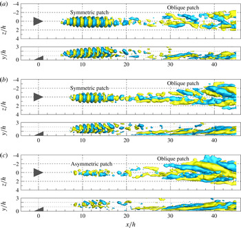


 Open access