


1. Introduction
Thermal convection is of crucial importance for understanding many thermally driven fluid flows in nature, for instance, ocean circulation, mantle convection and convections in celestial bodies. In certain circumstances involving convective flows, either the imposed temperature gradient has a non-parallel component with respect to gravity or the gravitational field itself is altered, resulting in an effective ‘horizontal buoyancy’ with respect to the temperature gradient, which makes the problem even more complicated; for example, mantle convection near the subduction zone (Taylor & Mclennan Reference Taylor and Mclennan1995; Wortel & Spakman Reference Wortel and Spakman2000; Ritter & Christensen Reference Ritter and Christensen2007), convection in binary star systems (Kenyon & Webbink Reference Kenyon and Webbink1984; Podsiadlowski, Joss & Hsu Reference Podsiadlowski, Joss and Hsu1992; Heintz Reference Heintz2012) and atmospheric circulation with wide latitude scales (Emanuel, Neelin & Bretherton Reference Emanuel, Neelin and Bretherton1994). In all these systems, a (significant) misalignment exists between the global temperature gradient and gravity.
A paradigm for studying thermal convection is the Rayleigh–Bénard convection (RBC) system (Ahlers, Grossmann & Lohse Reference Ahlers, Grossmann and Lohse2009; Lohse & Xia Reference Lohse and Xia2010; Chillà & Schumacher Reference Chillà and Schumacher2012; Xia Reference Xia2013), in which a fluid layer is heated at the bottom and cooled from above, therefore the global temperature gradient is strictly parallel to gravity. During the past few decades, a vast number of studies on turbulent RBC have been reported, focusing on various aspects of the system, such as heat transport, dynamics of the large-scale circulation, small-scale turbulence and the effect of complex boundary conditions.
A simple implementation of the horizontal buoyancy is to tilt the RB convection set-up by an angle  $\beta$ (figure 1). For small tilting angles, Ahlers, Brown & Nikolaenko (Reference Ahlers, Brown and Nikolaenko2006) found an increase of the speed in the large-scale circulation (LSC), but that increase does not significantly influence the heat transport efficiency. However, measurements in an aspect ratio $\varGamma = 0.5$ cell (Weiss & Ahlers Reference Weiss and Ahlers2013) reveal a very small increase of heat transport efficiency for tilt angle $\beta \approx 6^\circ$. This is in contradiction with the result of Chillà et al. (Reference Chillà, Rastello, Chaumat and Castaing2004), who reported a slight reduction of Nusselt number with the same aspect ratio but at higher Rayleigh numbers. Wei & Xia (Reference Wei and Xia2013) studied the properties of viscous boundary layers in RBC with tilt angles up to $\beta = 3.4^\circ$ in a cylindrical cell of $\varGamma = 1$. They found that for small tilt angles ( $\beta \le 1^\circ$), the scaling of viscous boundary layer thickness with the Reynolds number ( $Re$) is close to the Prandtl–Blasius laminar boundary layer scaling, while higher tilt angles result in a reduction in the scaling exponent.

Figure 1. (a) Comparison between the parameter space trajectory explored in the present study (red dashed line) and that by simply tilting the cell (black dashed curve, which is the case in most of the previous studies); panel (b) is a schematic drawing of the tilted cell. Here  $Ra_V$ is the vertical Rayleigh number and $Ra_H$ is the horizontal Rayleigh number (see (2.4) and (2.5) for definitions). Here RBC stands for ‘levelled’ RBC and VC stands for vertical convection (Ng, Chung & Ooi Reference Ng, Chung and Ooi2013; Ng et al. Reference Ng, Ooi, Lohse and Chung2015).
For convection with large tilt angles, sometimes also called the inclined layer convection, a number of studies (Daniels & Bodenschatz Reference Daniels and Bodenschatz2002; Daniels, Wiener & Bodenschatz Reference Daniels, Wiener and Bodenschatz2003; Daniels et al. Reference Daniels, Brausch, Pesch and Bodenschatz2008; Subramanian et al. Reference Subramanian, Brausch, Daniels, Bodenschatz, Schneider and Pesch2016) have been carried out to try to understand the spatio-temporally chaotic phenomenon and to identify different flow regimes near onset. Riedinger et al. (Reference Riedinger, Tisserand, Seychelles, Castaing and Chillà2013) studied the convection in a tilted channel connected by two chambers and identified four different flow regimes. Guo et al. (Reference Guo, Zhou, Cen, Qu, Lu, Sun and Shang2014) reported a monotonic decrease in Nusselt number for increasing  $\beta$ in a rectangular cell (aspect ratios $\varGamma _x = 1$ and $\varGamma _y = 0.25$). Jiang, Sun & Calzavarini (Reference Jiang, Sun and Calzavarini2019) conducted both experimental and numerical studies in a similar convection cell but with much higher Prandtl number ( $Pr$) and they reported a peculiar bimodal $Nu\text {--}\beta$ curve. For low Prandtl number, on the other hand, Frick et al. (Reference Frick, Khalilov, Kolesnichenko, Mamykin, Pakholkov, Pavlinov and Rogozhkin2015), Teimurazov & Frick (Reference Teimurazov and Frick2017) and Khalilov et al. (Reference Khalilov, Kolesnichenko, Pavlinov, Mamykin, Shestakov and Frick2018), using liquid sodium as working fluid, found that there exists an optimal tilting angle for heat transport. Shishkina & Horn (Reference Shishkina and Horn2016) and Zwirner & Shishkina (Reference Zwirner and Shishkina2018) conducted direct numerical simulations (DNS) for wide ranges of Rayleigh number, Prandtl number and different aspect ratios. They found that the normalized Nusselt number $Nu(\beta )/Nu(0)$ has a complicated, non-monotonic dependence on $\beta$ as well as $Ra$ and $Pr$. Recently, Wang et al. (Reference Wang, Wan, Yan and Sun2018b,Reference Wang, Xia, Wang, Sun, Zhou and Wanc) conducted two-dimensional DNS for tilted RBC with different aspect ratios. They identified multiple roll states for cells with large aspect ratios and studied the relationship between the different flow states and the global heat transport.
While these studies have clearly demonstrated the richness and complexities of the tilted RBC system, the complicated and sometimes seemingly contradictory results suggest the need for a different treatment of the effective horizontal buoyancy, which may offer a unifying understanding of the problem.
In the present study, unlike in most previous studies of tilted RBC, we fix the vertical thermal driving strength (in the cell frame) while varying the effective horizontal buoyancy over the vertical buoyancy (see figure 1). With this operation, we are able to systematically explore the effect of horizontal buoyancy while maintaining a non-zero vertical buoyancy. Experimentally, this is achieved by tilting the convection cell with respect to gravity by an angle  $\beta$ and simultaneously raise the temperature difference $\varDelta$ across the conducting plates by a corresponding amount.
The rest of the paper is organized as follows. In § 2, we first extend the classical Rayleigh–Bénard problem to the case in which an effective horizontal buoyancy is present. This section is further divided into three subsections: in § 2.1, we put forward the governing equations of the system; we then generalize the Nusselt number to a vector form in § 2.2 and thereby derive the expression for the global horizontal heat transfer. The exact balance relationships between the viscous dissipation rate, the thermal dissipation rate and the global heat transport are then derived in § 2.3. In § 3, details of the experimental set-up, and procedures of measurements and data analysis are provided. In particular, we propose in § 3.2 a new method to extract information about the LSC using the multiprobe temperature measurement data. As we use DNS to verify the experimental findings, a brief introduction of the DNS code used is presented in § 4. In § 5 we present and discuss both the experimental and numerical results. In § 6, we extend the Grossmann & Lohse (Reference Grossmann and Lohse2000, Reference Grossmann and Lohse2001, Reference Grossmann and Lohse2002) theory to the case in which an effective horizontal buoyancy is present. Finally, we summarize the present work in § 7.
2. Problem set-up
2.1. Governing equations
When the global temperature gradient and gravity are misaligned in a convective system (as with the case in tilted RBC), it can be described by the following governing equations:
 \begin{gather} \frac{\partial \boldsymbol{u}}{\partial t} + \boldsymbol{u}\boldsymbol{\cdot}\boldsymbol{\nabla}\boldsymbol{u} = -\frac{1}{\rho}\boldsymbol{\nabla} p + \nu\nabla^2\boldsymbol{u} + \alpha g\cos\beta(T-T_0)\hat{\boldsymbol{z}} + \alpha g\sin\beta(T-T_0)\hat{\boldsymbol{x}}, \end{gather}
 \begin{gather}\frac{\partial T}{\partial t} + \boldsymbol{u}\boldsymbol{\cdot}\boldsymbol{\nabla} T = \kappa\nabla^2T, \end{gather}
 \begin{gather}\boldsymbol{\nabla}\boldsymbol{\cdot} \boldsymbol{u} = 0, \end{gather}
where  $\beta$ is the angle between gravity and global temperature gradient, $\nu$ is the kinematic viscosity, $\kappa$ is the thermal diffusivity, $\alpha$ is the thermal expansion coefficient, $g$ is the acceleration due to gravity and $T_0$ is a reference temperature. Here, we have adopted the Oberbeck–Boussinesq approximation, in which all fluid properties are treated as independent of the temperature, except for the density in the buoyancy term. The Cartesian coordinate system is set in the frame of the convection cell (see figure 2a), such that $\hat {\boldsymbol {z}}$ is the ‘vertical’ unit vector pointing from the bottom plate to the top plate, $\hat {\boldsymbol {x}}$ is the ‘horizontal’ unit vector, and gravitational acceleration $\boldsymbol {g}$ lies in the $x$–
$x$– $z$ plane. Hereafter, all ‘vertical’ and ‘horizontal’ quantities mentioned are in the frame of the tilted cell.
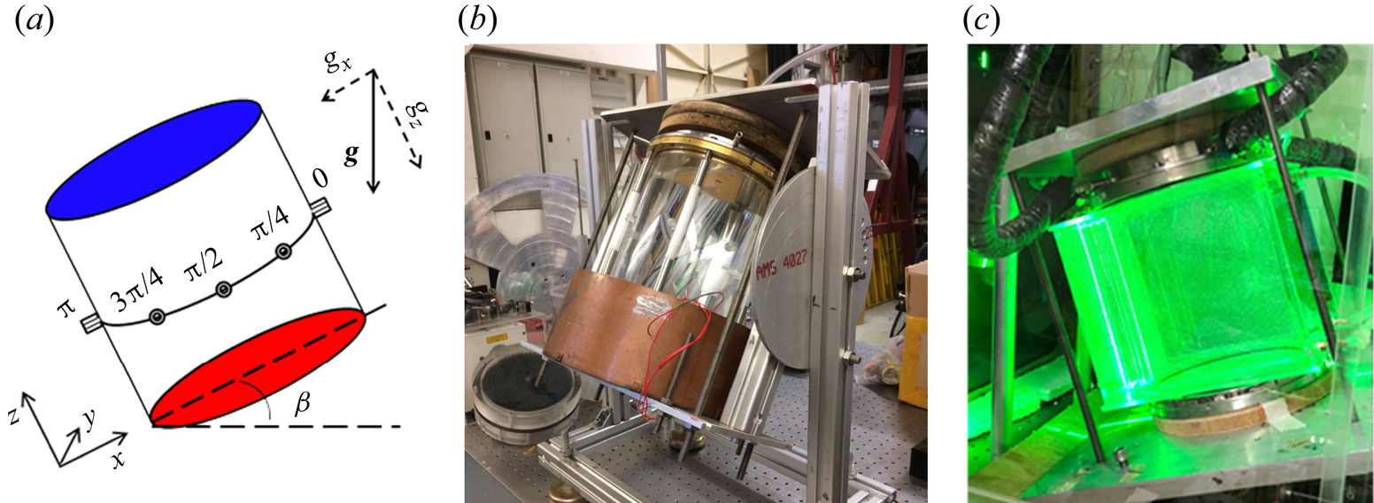
Figure 2. (a) Schematic drawing of the tilted RBC cell. The Cartesian coordinate system is set in the frame of the convection cell; (b) the large RBC cell with a home-made rotation frame; (c) the convection cell used for particle image velocimetry (PIV) measurement, a jacket filled with water is added to compensate the optical path to reduce image distortions.
In most previous tilted RBC studies, the tilting angle is increased while the temperature drop across the conducting plates is kept as a constant. This results in an increase in the effective horizontal buoyancy but a decrease in the vertical buoyancy. In the parameter space, this corresponds to an arc trajectory (the black dashed curve in figure 1). To explore the effect of horizontal buoyancy separately, we use  $\tau =\sqrt {H/(\alpha {\rm \Delta} g\cos \beta )}$ as the typical time scale (the free fall time for a fluid parcel to travel from the top plate to the bottom plate when the cell is tilted by an angle $\beta$), instead of $\tau =\sqrt {H/(\alpha {\rm \Delta} g)}$ (the conventional free fall time), together with the cell height $H$, the temperature difference $\varDelta$ across the two plates, to normalize the governing equations, which yields
 \begin{gather} \frac{\partial \tilde{\boldsymbol{u}}}{\partial \tilde{t}} + \tilde{\boldsymbol{u}}\boldsymbol{\cdot}\boldsymbol{\nabla}\tilde{\boldsymbol{u}} = -\boldsymbol{\nabla} \tilde{p} + \sqrt{\frac{Pr}{Ra_V}}\nabla^2\tilde{\boldsymbol{u}} + \tilde{T}\hat{\boldsymbol{z}} + \frac{Ra_H}{Ra_V}\tilde{T}\hat{\boldsymbol{x}}, \end{gather}
 \begin{gather}\frac{\partial \tilde{T}}{\partial \tilde{t}} + \tilde{\boldsymbol{u}}\boldsymbol{\cdot}\boldsymbol{\nabla} \tilde{T} = \sqrt{\frac{1}{Ra_V Pr}}\nabla^2\tilde{T}, \end{gather}
 \begin{gather}\boldsymbol{\nabla}\boldsymbol{\cdot} \tilde{\boldsymbol{u}} = 0, \end{gather}
where  $Ra_V \,{=}\,\alpha g\cos \beta {\rm \Delta} H^3\!/(\nu \kappa\!)$ is the vertical Rayleigh number, $Ra_H\,{=}\,\alpha g\sin \beta {\rm \Delta} H^3\!/(\nu \kappa\!)$ is the horizontal Rayleigh number and $Pr = \nu /\kappa$ is the Prandtl number. Note that by this definition, $Ra_V$ differs from the traditionally used $Ra = \alpha g {\rm \Delta} H^3 / (\nu \kappa )$ by a factor of $\cos \beta$, and it now represents the ‘vertical’ (with respect to the plates) thermal driving strength, as its name suggests. We stress that (2.4)–(2.6) are exactly the same as those of the traditional ‘levelled’ RBC except for an additional horizontal body force term in the momentum equation. For simplicity, we define $\varLambda = Ra_H/Ra_V = \tan \beta$ as the buoyancy ratio, which describes the relative strength of the effective horizontal buoyancy over the vertical one.
With this normalization, it is clear that when we tilt the convection cell by an angle  $\beta$, and accordingly raise the temperature difference across the conducting plates by a factor of $1/\cos \beta$, the vertical thermal forcing with respect to the cell is fixed (see the red dashed line in figure 1). This procedure enables us to use tilted RBC as a platform to explore the effect of horizontal buoyancy.
2.2. Generalization of the Nusselt number
Classical RBC is characterized by two response parameters, namely, the Nusselt number and the Reynolds number,
 \begin{gather} Nu = \frac{Q}{k\varDelta/H} = \frac{\langle u_zT\rangle_A - \kappa\partial_z\langle T\rangle_A}{\kappa\varDelta/H}, \end{gather}
 \begin{gather}Re = \frac{UH}{\nu}. \end{gather}
 In the above,  $Q$ is total vertical heat flux, $k$ is the thermal conductivity of the working fluid, $u_z$ is the vertical velocity and $\langle \cdot \rangle _A$ denotes averaging over any horizontal cross-section. The Nusselt number is a non-dimensional measurement of the total heat flux and the Reynolds number describes the relative flow strength (Sun & Xia Reference Sun and Xia2005).
In the presence of horizontal buoyancy, there exists a global horizontal heat transport. In such a case, the overall heat flux of the system must be represented by a vector. Following (2.7), we can readily write the vector form of the Nusselt number as
 \begin{equation} \boldsymbol{Nu} = \frac{\boldsymbol{Q}}{k\varDelta/H},\end{equation}
where the global heat flux  $\boldsymbol {Q}$ can be expressed in the integral form as
 \begin{equation} \boldsymbol{Q} = \frac{1}{V} \int\langle\boldsymbol{q}\rangle \, \textrm{d} V = \frac{c\rho}{V} \int \langle\boldsymbol{u} T - \kappa\boldsymbol{\nabla} T \rangle \, \textrm{d} V = - \frac{k}{V}\oint\langle\boldsymbol{r}\boldsymbol{\nabla} T\rangle\boldsymbol{\cdot} \textrm{d} \boldsymbol{S}. \end{equation}
 Here  $c$ is heat capacity and $\rho$ is the density of the working fluid. Physically, $\boldsymbol {Q}$ is just the volume-averaged local heat flux $\boldsymbol {q}$ over the whole convective domain. In the last step of (2.10), we have used the no-slip boundary conditions and applied Gauss's law. With $\hat {\boldsymbol {z}}$ being the unit vector pointing from the hot plate to the cold plate (see figure 1a), the vector form of Nusselt number $\boldsymbol {Nu}$ can be decomposed as
 \begin{equation} \boldsymbol{Nu} = \frac{(\hat{\boldsymbol{z}}\boldsymbol{\cdot}\boldsymbol{Q})\hat{\boldsymbol{z}} +(\hat{\boldsymbol{x}}\boldsymbol{\cdot}\boldsymbol{Q})\hat{\boldsymbol{x}}}{k\varDelta/H} = Nu_V\hat{\boldsymbol{z}} + Nu_H\hat{\boldsymbol{x}}. \end{equation}
 Here,  $Nu_V$ is the vertical component of $\boldsymbol {Nu}$ and $Nu_H$ is the horizontal component that represents the strength of the global horizontal heat transfer. In the last step of (2.11), we have used the fact that the acceleration due to gravity $\boldsymbol {g}$ lies in the $x$–
$x$– $z$ plane therefore the total heat flux $\boldsymbol {Q}$ should have no $y$ component, considering the reflection symmetry on the $y$ axis after taking ensemble average.
In the present study, the sidewall is adiabatic ( $\boldsymbol {\nabla } T\boldsymbol {\cdot } \textrm {d}\boldsymbol {S} = 0$), therefore the last integral in 2.10 survives only on the top and bottom surfaces. Substituting (2.10) into (2.11) we obtain
 \begin{gather} Nu_V = \frac{1}{V} \left.\left(\int_{z = 0}z \frac{\partial T}{\partial z} \, \textrm{d} S - \int_{z = H}z\frac{\partial T}{\partial z} \, \textrm{d} S \right)\right/(\varDelta/H) = - \frac{ \langle\partial T/\partial z\rangle_{z = H}}{\varDelta/H}, \end{gather}
 \begin{gather}Nu_H = \frac{1}{V} \left.\left(\int_{z = 0}x \frac{\partial T}{\partial z} \, \textrm{d} S - \int_{z = H}x\frac{\partial T}{\partial z} \, \textrm{d} S \right)\right/(\varDelta/H). \end{gather}
 Taking the adiabatic sidewall and no-slip boundary conditions into consideration, we can see that (2.12) is exactly the same as (2.7). While the definition of the horizontal Nusselt number  $Nu_H$ (2.13), on the other hand, can be interpreted as an integral of local heat flux at the plates weighted by its horizontal position.
The horizontal heat transfer is usually ignored in previous studies of tilted RBC. When horizontal buoyancy is non-zero, as we will see below, the global horizontal heat transfer is no longer negligible, and  $Nu_H$ becomes the third response parameter of the system. The non-zero horizontal heat flux may also be understood in term of a symmetry breaking, which will be discussed in detail in § 5.4.
We stress that the definitions in (2.12) and (2.13) are also applicable in other thermal convection systems. For example, thermal convection with mixed boundary conditions (Wang, Huang & Xia Reference Wang, Huang and Xia2017) (see figure 3b) and horizontal convection (Hughes & Griffiths Reference Hughes and Griffiths2008; Wang et al. Reference Wang, Huang, Zhou and Xia2016; Wang, Huang & Xia Reference Wang, Huang and Xia2018a) (figure 3c). For horizontal convection, since heating and cooling happen on the same height at the two ends of the cell, the vertical heat flux is always zero (see (2.12)), and only the horizontal component  $Nu_H$ survives.
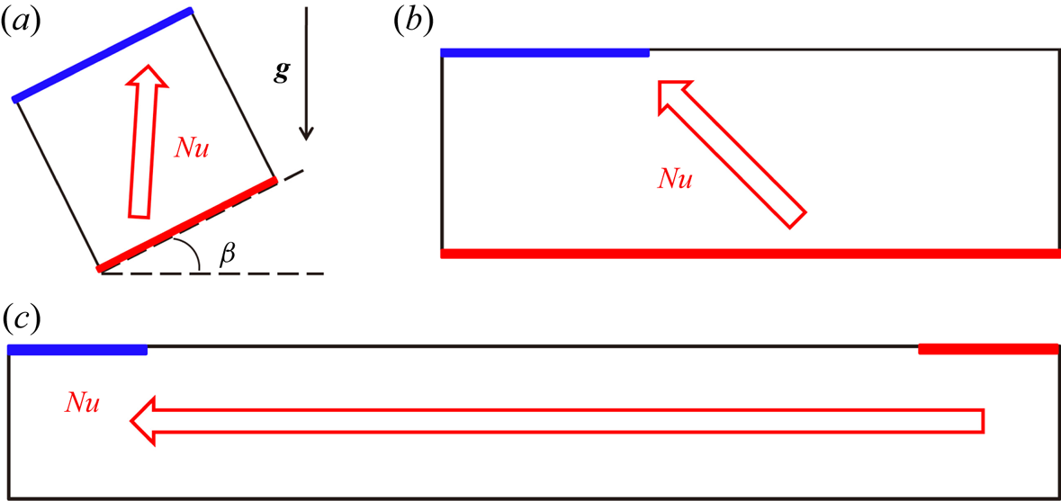
Figure 3. Schematic drawings of various thermal convection systems as well as their corresponding overall heat transfer direction (indicated by open arrows). (a) Tilted RBC; (b) thermal convection with mixed boundary conditions at the top plate; (c) horizontal convection.
2.3. Exact relations
The horizontal Nusselt number  $Nu_H$ makes the description of global heat transport more complete, it also alters the balance between global transfer properties and the dissipation rates. In the presence of horizontal buoyancy, the exact relations of volume-averaged viscous and thermal dissipation rates can be written as
 \begin{gather} \epsilon_u = \frac{\nu^3}{H^4}Ra_V Pr^{-2}(Nu_V - 1) + \frac{\nu^3}{H^4} Ra_H Pr^{-2} \left( Nu_H + \left\langle\frac{\partial \tilde{T}}{\partial \tilde{x}}\right\rangle_V\right), \end{gather}
 \begin{gather}\epsilon_\theta = \kappa\frac{\varDelta^2}{H^2}Nu_V, \end{gather}
where  $\langle \cdot \rangle _V$ denotes averaging over the whole convection domain. Comparing with RBC with just vertical buoyancy (Ahlers et al. Reference Ahlers, Grossmann and Lohse2009), there is now an additional term accounting for the contribution from the horizontal buoyancy in the exact relation for the energy dissipation rate (2.14). The thermal dissipation rate (2.15), on the other hand, depends only on the vertical Nusselt number and has the same form as in the classical case (because no additional term is involved in the energy equation, (2.5)), except that now the total Nusselt number is replaced by the vertical one.
3. Experiment set-up and procedures
3.1. The convection cell
A cylindrical convection cell with diameter  $D = 19.2$ cm and height $H = 20.0$ cm is used in the experiment, thus the aspect ratio $\varGamma = D / H$ is approximately unity (see figure 2b). The top and bottom plates are made of copper and the sidewall is made of Plexiglass with 4 mm thickness. Distilled and deionized water is used as working fluid. The top plate is cooled by a refrigerator and the bottom plate is heated by a resistive heater. The bulk temperature is set to be $T_{bulk} = 40\,^{\circ }$C, corresponding to a Prandtl number of $Pr = 4.3$. The whole convection cell is sat on a frame that is able to rotate along a horizontal axis.
Four thermistors (OMEGA Engineering, Model 44031/44032) are embedded in each plate to monitor the temperatures at the top and bottom boundaries. In addition, we embed eight thermistors equidistant around the midheight of the sidewall, to monitor the temperature signals therein and the LSC (Cioni, Ciliberto & Sommeria Reference Cioni, Ciliberto and Sommeria1997; Brown & Ahlers Reference Brown and Ahlers2006; Xi & Xia Reference Xi and Xia2007; Zhou et al. Reference Zhou, Xi, Zhou, Sun and Xia2009). The head of thermistor is only 0.2 mm away from the working fluid to minimize the possible filtering effect. A multichannel digital multimeter (Keysight, Model 36972A) is used to measure the resistances of these thermistors at a sampling rate approximately 0.75 Hz, the recorded resistances are then converted to temperature thereafter using the calibration data. An additional copper basin is applied to compensate for heat leakage from the bottom plate. Foam plastic, over 5 cm in thickness, is wrapped around the cell to prevent heat leakage from the sidewall. Finally, the whole rotating frame is placed into a home-made thermostat, whose temperature is set to be the same as the bulk temperature of the cell. The temperature stability of the thermostat is approximately  ${\pm }0.02$ K.
For the  $D = 19.2$ cm cell, measurements are conducted at three vertical Rayleigh numbers ( $Ra_V = 1.0\times 10^9$, $2.2\times 10^9$ and $4.6\times 10^9$) at six tilting angles $\beta = 0$, $20^{\circ }$, $30^{\circ }$, $40^{\circ }$, $50^{\circ }$ and $60^{\circ }$. The corresponding buoyancy ratios are $\varLambda = 0$, 0.36, 0.58, 0.84, 1.19 and 1.73, respectively. In order to expand the parameter range, we use another small cylindrical cell with $H = 9.9$ cm, whose aspect ratio is also around unity, to cover a lower vertical Rayleigh number range ( $Ra_V = 1.0\times 10^8$, $2.2\times 10^8$ and $4.6\times 10^8$). The corresponding tilt angles are the same as those of the larger cell. The sidewall of the small cell is made of glass, which suffers a severe heat leakage problem. A correction for the sidewall effect has been made to the data of the small convection cell, the details of the correction are described in § 3.3.
3.2. Sidewall temperature profile
In classical RBC, a commonly used method for extracting the information about the LSC is the so-called sinusoidal function method (SF) (Cioni et al. Reference Cioni, Ciliberto and Sommeria1997; Brown & Ahlers Reference Brown and Ahlers2006; Xi & Xia Reference Xi and Xia2007; Zhou et al. Reference Zhou, Xi, Zhou, Sun and Xia2009). This method fits the temperature signals at different azimuthal locations by  $T(\theta ) = T_0 + T_A\sin (\theta - \phi )$. Here, $T_0$ is the azimuthally averaged temperature, $T_A$ reflects the strength of the LSC and $\phi$ is the phase angle. The SF method has shown great success in studying the dynamics of the LSC, for example the meandering, cessation and reversal in RBC. Later, Zhou et al. (Reference Zhou, Xi, Zhou, Sun and Xia2009) developed a temperature-extrema-extraction (known as TEE) method, based on which they identified a novel sloshing mode of the LSC (Xi et al. Reference Xi, Zhou, Zhou, Chan and Xia2009).
With the presence of effective horizontal buoyancy ( $\varLambda > 0$), the azimuthal temperature profile may change and an SF description might not be accurate. For this reason, we introduce in this section a closed-form expression for the azimuthal temperature profile, which not only gives a better description of the measured temperature profile, but also quantifies the degree of coherency of the LSC.
As the first step, we modify the sinusoidal function by using the trigonometric identity  $\sin \theta = 2\tan (\theta /2)/[1+\tan ^2(\theta /2)]$ and substitute $\tan (\theta /2)$ with $b\tan (\theta /2)$, giving
 \begin{equation} T(\theta) = T_0 + T_A\times\frac{2b\tan\left(\dfrac{\theta-\phi}{2}\right)}{1 + b^2\tan^2\left(\dfrac{\theta-\phi}{2}\right)},\end{equation}
where  $b > 0$ is a parameter which is related to the off-centre distance of the LSC (Zhou et al. Reference Zhou, Xi, Zhou, Sun and Xia2009). One can easily verify that the maximum temperature in (3.1) occurs at $\theta _{T,max} = 2\arctan (1/b) + \phi$ and the minimum temperature at ${\theta _{T,min} = 2\arctan (-1/b) + \phi}$. The off-centre distance of the line connecting these two points is
 \begin{equation} d = R\sin[2\arctan(1/b)-{\rm \pi}/2], \end{equation}
where  $R$ is the radius of the convection cell, and the sloshing mode can be exclusively captured when $b$ is determined.
For the second step, considering that the horizontal buoyancy may separate the hot and cold plumes and form highly concentrated hot/cold angular regions, we incorporate a power law function and finally obtain the expression of the temperature profile as
 \begin{equation} T(\theta) = T_0 + T_A\times\frac{2b\tan\left(\dfrac{\theta-\phi}{2}\right)}{1 + b^2\tan^2\left(\dfrac{\theta-\phi}{2}\right)}\left| \frac{2b\tan\left(\dfrac{\theta-\phi}{2}\right)}{1 + b^2\tan^2\left(\dfrac{\theta-\phi}{2}\right)}\right|^\zeta,\end{equation}
where  $\zeta > -1$ is the second parameter that describes the shape of the profile. Other parameters, $T_0$, $T_A$ and $\phi$, as in the SF method, denote the mean temperature, the amplitude and the phase angle of the LSC. One can check that when $b = 1$ and $\zeta = 0$, (3.3) reduces to a sinusoidal function.
Figure 4(a) shows an example of the measured instantaneous azimuthal temperature profile at the midheight of the large convection cell. The open circles are the temperature signals of the eight thermistors and the red solid line shows the power law half-angle formula fitting (PHAF) curve. For comparison, we plot in the same figure the SF fitting by a black dashed line. It is clearly seen that the PHAF method gives a better description of the instantaneous profile.
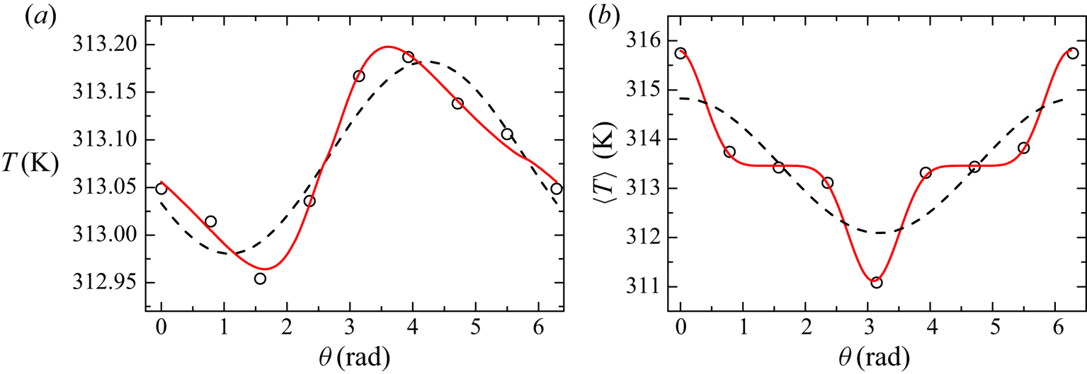
Figure 4. (a) Instantaneous azimuthal temperature profile at midheight of the sidewall measured by the eight thermistors at  $Ra_V = 4.6 \times 10^9$, $Pr = 4.3$, $\varLambda = 0$, (open circles); fitting by the proposed function (3.3), (solid line); a sinusoidal fitting, (dashed line). (b) Mean temperature profile at $Ra_V = 4.6\times 10^9$, $Pr = 4.3$ and buoyancy ratio $\varLambda = 0.84$, (open circles); fitting by a power law sinusoidal function (3.4), (solid line); a sinusoidal fitting, (dashed line).
The other parameter  $\zeta$, describes the azimuthal range spanned by the hot ascending flow and the cold descending flow. A large value of $\zeta$ corresponds to a narrow hot/cold range and vice versa. Figure 4(b) shows an example of the time averaged azimuthal temperature profile at $Ra_V = 4.6\times 10^9$, $Pr = 4.3$ and $\varLambda = 1.73$. In the presence of the horizontal buoyancy, we can see that the hot/cold plumes indeed move towards the sidewall region and the hot/cold plumes are confined in a narrower angular range compared with the $\varLambda = 0$ case. As a result, the LSC is locked in the $x$–
$x$– $z$ plane. Since the reflection symmetry about the $y$ axis is not affected by the horizontal buoyancy, after taking the long-time average, the points with maximum and minimum temperatures of the profile should lie in the $x$–
$x$– $z$ plane. For simplicity, hereafter we fix $b = 1$ (corresponding to the off-centre distance $d = 0$) for all time-averaged (over one and a half hours for all runs) temperature profiles. Substituting $b = 1$ into (3.3), it reduces to
 \begin{equation} T(\theta) = T_0 + T_A\sin(\theta - \phi)\times|\sin(\theta - \phi)|^\zeta. \end{equation}
 The red solid line in figure 4(b) shows the fitting result of (3.4) for the time averaged case. For comparison, the sinusoidal fitting is also plotted by the dashed line. Clearly, (3.4) gives a more accurate description of the profile than the SF methods, i.e. all eight experimental data points fall on the solid curve. It is also evident that the horizontal buoyancy traps both the hot ascending and cold descending flows in a smaller angular region, which implies that the ‘coherency’ of the plumes is increased. This feature can also be reflected by the full width at half-maximum (FWHM) of the profile, which is related to  $\zeta$ as
 \begin{equation} \textrm{FWHM} = 2\arccos[2^{-1/(1+\zeta)}]. \end{equation}
 Note that the FWHM as given above is a monotonic decreasing function of  $\zeta$. For temperature profiles with higher $\zeta$ value, the hot and cold plumes are highly concentrated at the opposite sides of the sidewall. For this reason, we refer to $\zeta$ as the ‘coherency index’.
3.3. Sidewall correction
Since the sidewall of the small convection cell is made of glass, whose thermal conductivity ( $1.1\ \textrm {W}\ (\textrm {m}\ \textrm {K})^{-1}$) being much higher than that of Plexiglass ( $0.19\ \textrm {W} (\textrm {m}\ \textrm {K})^{-1}$), the sidewall heat leakage makes a considerable contribution to the measured overall heat transfer. To subtract this additional heat transfer, we adopt the correction proposed by Roche et al. (Reference Roche, Castaing, Chabaud, Hébral and Sommeria2001). The central idea is to consider that the vertical temperature profile decreases exponentially in the sidewall and the characteristic length scale of profile, which also accounts for the sidewall heat leakage, can be expressed as
 \begin{equation} \lambda = \frac{AR\sqrt{2}}{2}\left(\frac{W}{\varGamma Nu_V}\right)^{1/2}, \end{equation}
where  $R$ is the radius of the conducing plate; $\varGamma$ is the aspect ratio of the cell; $A$ is a constant of order unity, we use the value $A = 0.8$ proposed by Roche et al. (Reference Roche, Castaing, Chabaud, Hébral and Sommeria2001) throughout this work; $W$ is the wall number, defined as the ratio between empty cell heat conductivity and the quiescent fluid heat conductivity,
 \begin{equation} W = 2k_We/k_fR,\end{equation}
where  $k_W$ and $k_f$ are the thermal conductivity of the wall material and the working fluid, respectively; $e$ is the thickness of the sidewall. Putting everything together, one can obtain the relation between the corrected Nusselt number and the measured one as
 \begin{equation} Nu_{V,cor} = Nu_{V,mea}\left/\left[1 + A\sqrt{2}\left(\frac{W}{\varGamma Nu_{V,cor}}\right)^{1/2}\right]\right. . \end{equation}
3.4. Flow field measurements
In addition to the heat transport measurements, we also use the PIV technique to quantify the flow fields. Figure 2(c) shows a photo of the convection cell used for PIV measurement. To minimize the effect of optical distortion, we add a rectangular jacket to the sidewall, which is filled with distilled and deionized water. A Litron Nd:YAG 532 nm laser is used for illumination. The light sheet is approximately 2 mm in thickness and illuminates the vertical cross-section of the cell through the centreline. Dantec PSP polyamid particles (with diameter  $d = 50\ \mathrm {\mu }$m) are used as seeding particles. The centre temperature of the convection cell is also set to be 40 $^\circ$C. The vertical Rayleigh number is set to be $Ra_V = 4.8\times 10^9$, which is close to the highest value in our heat transport measurement. The whole set-up is placed into another transparent home-made thermostat with its temperature set to be the same as the bulk temperature. Each image sequence is recorded at a frame rate of $f = 15$ Hz and lasts for 30 minutes, consisting of $27\,000$ raw images. The velocity field is calculated afterwards for each tilting angle using the single frame mode. Six sets of measurements with buoyancy ratio $\varLambda = 0$, 0.36, 0.58, 0.84, 1.19 and 1.73 are made, corresponding to tilting angles $\beta = 1^\circ$, 20 $^\circ$, 30 $^\circ$, 40 $^\circ$, 50 $^\circ$ and 60 $^\circ$, respectively. For the case of $\varLambda = 0$, we deliberately tilt the cell by $\beta = 1^\circ$. Such small tilt angle ( $\beta = 1^\circ$) can lock the LSC in the $x$–
$x$– $z$ plane without inducing a noticeable change in the flow strength compared with the strictly levelled case (Ahlers et al. Reference Ahlers, Brown and Nikolaenko2006; Wei & Xia Reference Wei and Xia2013).
4. Direct numerical simulations
To verify the experimental results, we conduct DNS with the same parameter settings. In addition, the Prandtl number effect is also explored at fixed vertical Rayleigh number  $Ra_V = 10^8$. We adopt the CUPS code (Chinese University of Hong Kong pencil code simulation for turbulent convection (Kaczorowski & Xia Reference Kaczorowski and Xia2013; Kaczorowski, Chong & Xia Reference Kaczorowski, Chong and Xia2014; Chong, Ding & Xia Reference Chong, Ding and Xia2018)) to solve (2.4)–(2.6) using a fourth-order finite-volume method on staggered grids. All simulations are conducted in a cylindrical domain with aspect ratio equal to unity. All boundaries are set to be impermeable and non-slip. The sidewall is adiabatic while constant temperature conditions are applied at both the top and bottom plates. A non-uniform mesh with denser grids at all boundaries is adopted for both the temperature and velocity fields. A multiresolution scheme in which the temperature mesh is denser than the velocity mesh (see appendix A) is also used to save the computational cost of the simulations at high Prandtl numbers. For a detailed description of the code, we refer to Chong et al. (Reference Chong, Ding and Xia2018).
5. Results and discussions
5.1. The global heat transfer
In figure 5, we plot the vertical Nusselt numbers as a function of the buoyancy ratio (and the horizontal Rayleigh number). Open and solid circles represent experimental data with and without sidewall corrections, respectively. The DNS data are shown as open triangles. It is seen that our experimental results show good agreement with the DNS data. For the six vertical Rayleigh numbers measured,  $Nu_V$ increases monotonically with the buoyancy ratio $\varLambda$. In other words, the horizontal buoyancy facilitates the vertical heat transport, at least in a closed cylindrical convection domain with aspect around unity. This finding is different from most previous studies on tilted RBC (Guo et al. Reference Guo, Zhou, Cen, Qu, Lu, Sun and Shang2014; Shishkina & Horn Reference Shishkina and Horn2016; Teimurazov & Frick Reference Teimurazov and Frick2017; Jiang et al. Reference Jiang, Sun and Calzavarini2019). The main reason is that we have adopted a different normalization scheme and our experiment follows a straight line in the parameter space shown in figure 1.

Figure 5. The vertical Nusselt number ( $Nu_V$) as a function of the buoyancy ratio ( $\varLambda$) for different vertical Rayleigh numbers ( $Ra_V$). The top axes show the corresponding horizontal Rayleigh numbers. Circles are the experimental data and triangles represent the DNS data. Open and solid symbols represent data with and without sidewall corrections, respectively. The experimental data in panels (a–c) are measured using the small cell and correspond to $Ra_V = 1.0, 2.2$ and $4.6 \times 10^8$, respectively; the data in panels (d–f) are taken from the large cell, the corresponding vertical Rayleigh numbers are $Ra_V = 1.0, 2.2$ and $4.6 \times 10^9$.
To obtain the horizontal Nusselt number (2.13), we need to have the distribution of temperature gradient on both plates, which is very difficult for the experiment but readily available in DNS. We plot the calculated horizontal Nusselt numbers from DNS in figure 6. Points at  $\varLambda = 0$ are omitted since in such a case, the dynamics of the LSC (e.g. reversal, cessation and meandering) will result in a zero mean horizontal transport. The absolute value of $Nu_H$ is an order of magnitude smaller than $Nu_V$ for the parameter range explored, which means that the overall heat transport, defined by (2.11), is always dominated by the vertical component. For all data sets, the horizontal Nusselt also shows a general increasing trend with the buoyancy ratio. A small bump is seen for some vertical Rayleigh number ( $Ra_V = 1.0\times 10^8, 1.0\times 10^9$ and $4.6\times 10^9$) at the lower end of the curve. We do not know the exact reason for such a bump, it may be related to the change in the overall flow structure (see § 5.4).

Figure 6. The DNS result of horizontal Nusselt number ( $Nu_H$) as a function of the buoyancy ratio ( $\varLambda$) for different vertical Rayleigh numbers ( $Ra_V$). The top axes show the corresponding horizontal Rayleigh numbers. The corresponding vertical Rayleigh number in each subplot is the same as figure 5.
To see the relative enhancement more clearly, we plot the vertical Nusselt number as a function of the buoyancy ratio  $\varLambda$ for six different Rayleigh numbers $Ra_V$ in figure 7(a). Furthermore, to quantify the relative increase in vertical heat transport, we normalize the vertical Nusselt number with the value of the levelled case $Nu_V(0)$. The results are plotted in figure 7(b) with the same symbols. For all six vertical Rayleigh numbers, the relative enhancements of vertical heat transfer, $Nu_V(\varLambda )/Nu_V(0)$, almost follow the same trend. A linear fitting of all the data points gives $Nu_V(\varLambda )/Nu_V(0) = 1 + 0.14\varLambda$, which is also plotted as the solid line in figure 7(b). The maximum deviation from this line is approximately 2.5 $\%$.
$\%$.

Figure 7. (a) Experimentally measured vertical Nusselt number as function of the buoyancy ratio  $\varLambda$. From top to bottom, the corresponding vertical Rayleigh numbers are $Ra_V = 4.6\times 10^9$, $2.2\times 10^9$, $1.0\times 10^9$, $4.6\times 10^8$, $2.2\times 10^8$, $1.0\times 10^8$, respectively. Note for the last three sets of data, sidewall correction has been made. (b) Normalized Nusselt number as a function of the buoyancy ratio. The symbols are the same as those in panel (a). The solid line shows a linear fitting with $Nu_V(\varLambda )/Nu_V(0) = 1 + 0.14\varLambda$.
In previous studies on turbulent RBC, the two response parameters,  $Nu$ and $Re$, are often described by an effective scaling law on both Rayleigh number and Prandtl number (Siggia Reference Siggia1994; Grossmann & Lohse Reference Grossmann and Lohse2000, Reference Grossmann and Lohse2001, Reference Grossmann and Lohse2002). To check whether the power law scaling of vertical Nusselt number is still valid when horizontal buoyancy is presented, we plot $Nu_V$ as a function of the vertical Rayleigh number
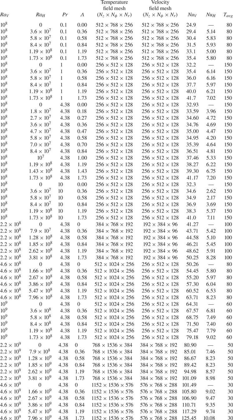
  $Ra_V$ in figure 8(a). A compensated plot is also shown in figure 8(b). Different symbols correspond to different horizontal buoyancy strength. In the same figure, we also plot the results of power law fittings with solid lines. The scaling exponents and the magnitudes are summarized in table 1. One sees that for a fixed buoyancy ratio $\varLambda$, the vertical heat transports ranges from 0.283 to 0.293, the small fluctuation in scaling exponent may result from the use of two different convection cells and the intrinsic uncertainty of the measurement. We conclude that the buoyancy ratio does not have an evident effect on the scaling exponents.

Figure 8. (a) Measured vertical Nusselt number as a function of vertical Rayleigh number. Solid lines are power law fittings to the data. (b) Compensate plot of vertical Nusselt number by  $Ra_V^{0.29}$, the legends are the same as those in panel (a).
Table 1. Power law fitting parameters of  $Nu_V = A\times Ra_V^\gamma$ from the experimental data for different buoyancy ratios.

Generally speaking, our experimental results show that the effect of horizontal buoyancy on vertical heat transfer is two-sided. Firstly, increasing the horizontal buoyancy results in a monotonic increase of  $Nu_V$, which can be approximated as a linear function as
 \begin{equation} Nu_V(\varLambda)/Nu_V(0) = 1 + 0.14\varLambda. \end{equation}
 Secondly, for a fixed buoyancy ratio up to  $\varLambda = 1.73$, the $Nu_V$– $Ra_V$ scaling is not affected by the horizontal buoyancy. We then propose two qualitative explanations for this monotonic enhancement. The first one is from the view of energy balance of the exact relations, as we have already discussed in § 2.3. The second one is from the point of view of plume coherency. When horizontal buoyancy sets in, it will push the ascending hot plumes near the bottom plate to the right and the descending cold plumes near the top plate to the left. The hot/cold plumes will then aggregate, merge and condense on the opposite sides, forming a large bundle of plumes that are more coherent, contain more heat, and finally increase the overall vertical heat transport (Huang et al. Reference Huang, Kaczorowski, Ni and Xia2013). To verify this assumption, information about the temperature field as well as the velocity field is required.
5.2. Temperature profile at midheight of the cell
The experimentally measured azimuthal mean temperature profiles for six buoyancy ratios are plotted in figure 9. The vertical Rayleigh number is  $Ra_V = 4.6\times 10^9$. The local temperatures are measured by the eight thermistors placed equidistant at the midheight of the sidewall and averaged over more than 90 minutes. The solid lines in figure 9 show the fitting results of (3.4). It is seen that for large $\varLambda$ value, the normalized temperature contrast, $\tilde {T}_A$, also increases. Meanwhile, the angular range covered by the hot/cold plumes, seems to decrease first (for $\varLambda$ up to 0.58), and then saturates at higher values of $\varLambda$. The flat shoulder suggests that the plumes become increasingly confined spatially with increasing effective horizontal buoyancy (this is related to the flow dynamics, i.e. the azimuthal range of the LSC is reduced). The error bar represents the standard deviation of temperature fluctuation at each measurement point. The overall temperature fluctuations decrease for increasing buoyancy ratio, which suggests that the overall flow is more stable. A close inspection reveals that the fluctuations are highest at $\theta = 0$ and ${\rm \pi}$, corresponding to where most of the hot plumes are moving upward and cold ones moving downward, respectively. For comparison, we plot in the same figure the mean temperature profiles obtained from DNS shown as shaded curves, with the width representing the corresponding standard deviation. It is seen that the DNS results in general agree well with our experimentally measured profiles, except for the levelled case ( $\varLambda = 0$), for which the LSC does not necessarily stay in the $x$–
$x$– $z$ plain. For the highest buoyancy ratio, the fitting curves and the DNS profiles start to show some deviation. Nevertheless, the experimental points remain on both curves. This indicates that in such a case, eight thermistors might not be sufficient to describe the temperature profile.

Figure 9. The solid circles are the experimentally measured mean temperature profile at midheight of the sidewall (normalized by the temperature difference across the plates) for different horizontal buoyancy strength ( $Ra_V = 4.6\times 10^9$, $Pr = 4.3$). The temperature standard deviations are denoted by error bars. The solid lines are fits of (3.4) to the experimentally measured data. The shaded curves are the corresponding mean temperature profiles from DNS, with the width of the curve representing the corresponding standard deviation.
The fitting parameters for the solid curves in figure 9 are plotted in figure 10. It is seen that the relative amplitude  $\tilde {T}_A$ of the temperature profile increases as we increase the horizontal buoyancy $\varLambda$ (figure 10a). The behaviour of $\zeta$ (figure 10b) is a bit more complicated, it is around zero for the first two buoyancy ratios, and increases rapidly for $\varLambda > 0.36$, while for the largest $\varLambda$ explored in our experiment it drops again. For a clear view, we convert $\zeta$ to the FWHM of the profile using (3.5), the results are then plotted in figure 10(c). For the first three points, the FWHM decreases rapidly, while for higher $\varLambda$, the change in FWHM is small. This is consistent with our qualitative description in figure 9. As a matter of fact, after obtaining these fitting parameters, we are able to estimate the strength of horizontal heat transfer, for details see appendix 3.

Figure 10. (a) Normalized amplitude of the temperature contrast  $\tilde {T}_A = T_A/\varDelta$ as a function of the buoyancy ratio $\varLambda$, (b) the coherency index $\zeta$ and (c) FWHM of each profile. The corresponding vertical Rayleigh number is $Ra_V = 4.6\times 10^9$.
5.3. The mean flow field measured by PIV
In order to quantify the change in the flow field, we conducted PIV measurements. We first plot the coarse grained mean velocity fields in figure 11, with the colourbar denoting the magnitude of the velocity vector. Each field is averaged over  $27\,000$ velocity maps to ensure statistical convergence.

Figure 11. Experimentally measured mean velocity fields for different buoyancy ratios at vertical Rayleigh number  $Ra_V = 4.8\times 10^9$. The colourbar denotes velocity magnitude.
For the strictly levelled case ( $\varLambda = 0$), the LSC undergoes azimuthal, torsional and sloshing motion (Funfschilling & Ahlers Reference Funfschilling and Ahlers2004; Sun, Xi & Xia Reference Sun, Xi and Xia2005; Brown & Ahlers Reference Brown and Ahlers2006; Xi, Zhou & Xia Reference Xi, Zhou and Xia2006; Xi & Xia Reference Xi and Xia2008; Xi et al. Reference Xi, Zhou, Zhou, Chan and Xia2009; Zhou et al. Reference Zhou, Xi, Zhou, Sun and Xia2009). In order to lock the LSC in the PIV measurement plane, we tilted the cell slightly by $\beta = 1^\circ$ (corresponding to $\varLambda = 0.02$), which will serve as a baseline for the ‘levelled’ case. It is seen from figure 11 that in this case the flow near the sidewalls (where the plumes are abundant) is intense and the centre of the cell remains quiescent. Also, the LSC is elliptical, with its long axis along the diagonal of the cross-section, which is similar to previous observations for nominally levelled cases ( $\varLambda \approx 0$) (Xia, Sun & Zhou Reference Xia, Sun and Zhou2003; Guo et al. Reference Guo, Zhou, Cen, Qu, Lu, Sun and Shang2014). As the horizontal buoyancy $\varLambda$ increases, one sees a remarkable change in the flow field. The LSC becomes more robust with increasing $\varLambda$, and expands towards the sidewall region, resulting in a square-like structure. The cold plumes detach from the top left-hand corner, accelerate towards the bottom plate, and reach their maximum velocity at the left-hand bottom corner. The hot plumes, on the other hand, reach their maximum velocity around the top right-hand corner. The bulk region remains almost stagnant for all the buoyancy ratios explored, and the area of this quiescent region is seen to increase with $\varLambda$.
Unfortunately, in our PIV measurement, the jacket fitted to the outside of the sidewall blocks the light scattered from the seeding particles near both the top and bottom plates, so we are not able to measure the velocity boundary layer. But a general feature of the mean wind can still be identified. With increasing buoyancy ratio, the mean ‘wind’ below (above) the top (bottom) plate becomes more confined. In figure 12, we show the magnitude of the mean vertical velocity at different buoyancy ratios. The hot ascending flow on the right-hand side and cold descending flow on the left-hand side are indeed separated by the horizontal buoyancy, aggregating on both sides of the sidewall. This finding is in line with our temperature profile measurements, suggesting that the plumes are more coherent.

Figure 12. Experimentally measured mean vertical velocity fields for different buoyancy ratios at vertical Rayleigh number  $Ra_V = 4.8\times 10^9$.
Our PIV measurement reveals that the horizontal buoyancy can effectively increase the flow strength, especially the vertical velocity in the plume dominated sidewall region in the  $x$–
$x$– $z$ plane.
5.4. Temperature and velocity fields
In figure 13, we plot the instantaneous temperature isosurfaces from DNS for different buoyancy ratios at vertical Rayleigh numbers  $Ra_V = 10^8$ and $Ra_V = 10^9$, respectively. The general feature of the flow structures in these two $Ra_V$ sets are similar: the large-scale circulation expands towards the perimeter of the cell as the buoyancy ratio is increased; the areas of cold-plume impacting and hot-plume ejecting regions at the bottom (and vice versa for the top plate) also seem to decrease, resulting in a larger shear dominated region in the centre of the bottom (top) plate.

Figure 13. Snapshots of temperature isosurfaces (from DNS) for vertical Rayleigh numbers  $Ra_V = 10^8$ (upper) and $10^9$ (lower) at different buoyancy ratios. The Prandtl number is $Pr = 4.38$.
We plot the temperature snapshots in the  $x$–
$x$– $z$ plane together with the velocity fields for different horizontal buoyancy strength in figure 14(a) and their corresponding mean fields in figure 14(b). The vertical Rayleigh number is fixed at $Ra_V = 10^8$. The flow fields show similar features as our PIV results (figures 11 and 12), although the vertical Rayleigh numbers differ by over one order of magnitude. Moreover, near the top/bottom plate, where PIV measurement is not accessible, we can see a region with high horizontal velocity. The height of the high-velocity region decreases with increasing buoyancy ratio. The temperature contrast of the cold and hot plumes increases with $\varLambda$. This again is in agreement with our temperature profile measurements (figure 10).
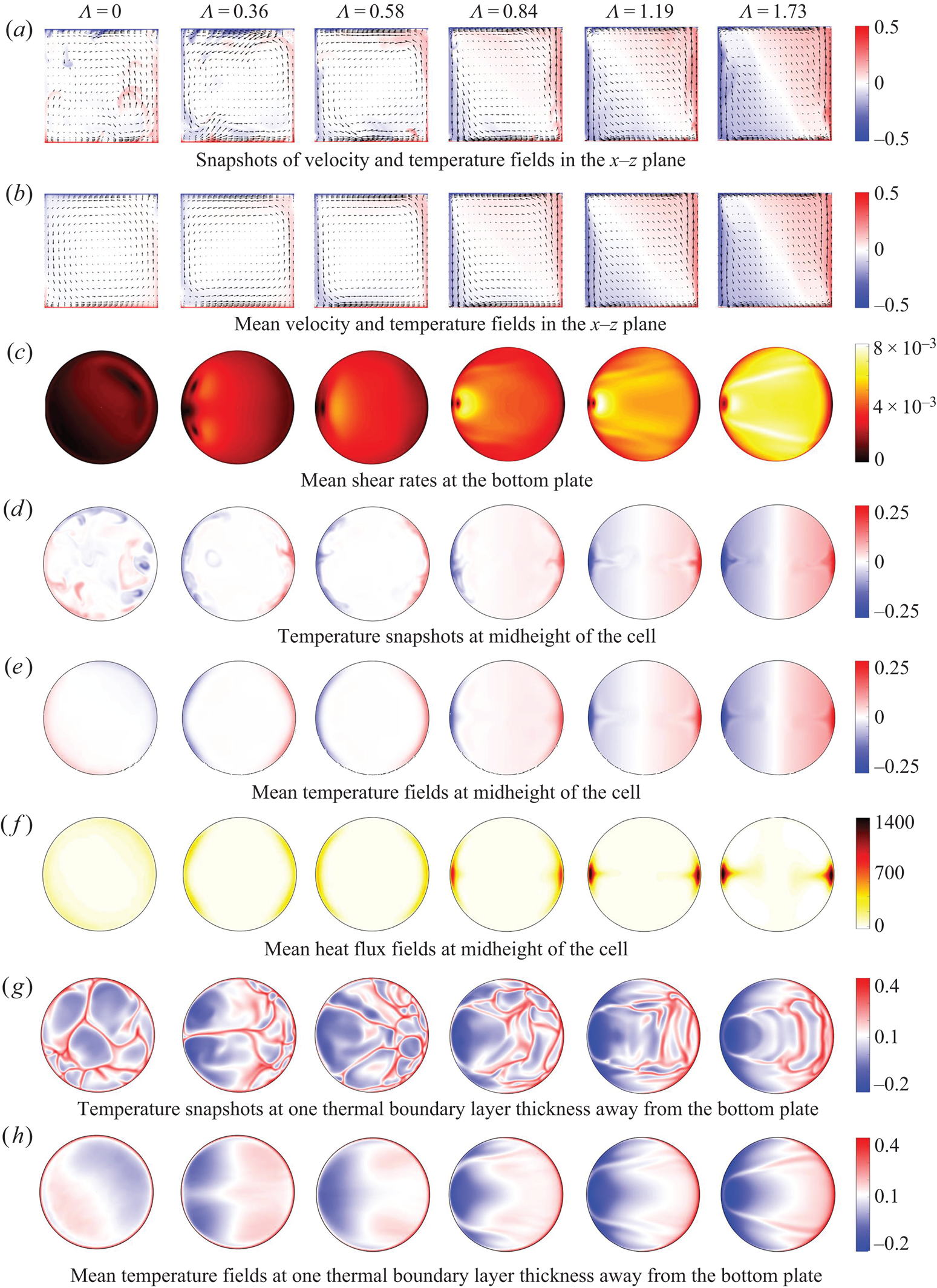
Figure 14. Cross-sections of various quantities (from DNS) for buoyancy ratios  $\varLambda = 0$, 0.36, 0.58, 0.84, 1.19 and 1.73 at vertical Rayleigh number $Ra_V = 10^8$ and Prandtl number $Pr = 4.38$. (a) Snapshots of temperature and velocity fields in the $x$–
$x$– $z$ plane; (b) mean temperature and velocity fields in the $x$–
$x$– $z$ plane; (c) mean shear rates at the bottom plate; (d–f) temperature snapshots, mean temperature and mean heat flux field at midheight of the cell; (g,h) snapshots and mean temperature fields at one thermal boundary layer thickness away ( $z = \delta _T$) from the bottom plate.
Figure 14(c) shows the mean shear rate at the bottom plate. We can see that the shear rate increases dramatically with increasing buoyancy ratio. For large  $\varLambda$ values, a strong horizontal wind sweeps over the bottom plate, which directly thins the thermal boundary layer.
In addition, we plot both the instantaneous and mean temperature fields of horizontal cross-section at midheight of the convection cell in figures 14(d) and 14(e), respectively. For the case with  $\varLambda = 0$, the cold and hot plumes are randomly distributed and are able to meander azimuthally. At small $\varLambda$ values, the cold and hot plumes start to move towards opposite sides, forming a cold and a hot spot at the two sides, respectively. Within these spots, the temperature and vertical velocity are highly correlated, resulting in an extremely enhanced local heat flux (Xia, Xin & Tong Reference Xia, Xin and Tong1995; Shang, Tong & Xia Reference Shang, Tong and Xia2008). These heat transport ‘channels’ can be clearly seen in figure 14(f), in which we plot the mean heat flux field at the midheight. Mean local flux as high as 1400 is observed for the highest $\varLambda$, which is approximately $30$ times the global averaged vertical Nusselt number.
Figures 14(g) and 14(h), respectively, show the horizontal cross-section of the instantaneous and mean temperature fields at the vertical position corresponding to one thermal boundary layer thickness ( $z = \delta _T$) near the bottom plate for different buoyancy ratios. For the case with $\varLambda = 0$, sheet-like plumes are randomly distributed at the bottom plate (Zhou, Sun & Xia Reference Zhou, Sun and Xia2007; Zhou & Xia Reference Zhou and Xia2010). Whereas, with increasing $\varLambda$, bundles of cold plumes impinge on the left-hand side of the bottom plate, forming a large cold area. The hot sheet-like plumes, on the other hand, are pushed to the right-hand side, and emit incessantly therein. For the two highest values of $\varLambda$ (the two right-most panels of figure 14g), the sheet-like plumes propagate towards the right-hand side in a wavy-like manner. The mean temperature fields are therefore highly inhomogeneous, with the left-hand side being much colder than the right-hand side (figure 14h). Note that for levelled RBC, the governing equations satisfy the reflection symmetry about the $y$–
$y$– $z$ plane ( $u_x \rightarrow -u_x, x \rightarrow -x$). In other words, if $(T, u_x, u_y, u_z)$ is the solution of (2.1)–(2.3), so is $(T^\prime , u_x^\prime , u_y^\prime , u_z^\prime )(x,y,z) = K_x(T, u_x, u_y, u_z)(x,y,z) = (T, -u_x, u_y, u_z)(-x,y,z)$. Therefore the ensemble average of the temperature fields, and the temperature gradient on both plates, should also satisfy the $K_x$ symmetry and the horizontal Nusselt is always zero (2.13). However, a non-zero $\varLambda$ (i.e. the last term on the right-hand side of (2.1)) breaks this symmetry. It is indeed the breaking of the $K_x$ symmetry that gives rise to the observed global horizontal heat transfer (2.13). It is also worth mentioning that, it appears that the difference between the integral on the top and bottom plates determines the magnitude of $Nu_H$. In fact, the system conserves the $K_{xz}$ symmetry ( $u_x \rightarrow -u_x, u_z \rightarrow -u_z, T \rightarrow -T, x \rightarrow -x, z \rightarrow -z$) even in the case of non-zero buoyancy ratio. This means that if one takes the ensemble average, the two surface integrals on the right-hand side of (2.13) are equal in magnitude and only differ by a sign, and the integral at both plates contribute equally to the overall $Nu_H$. (In appendix 2, we will show rigorously that the properties of vanishing $Nu_H$ in the case of levelled RBC, and non-zero $Nu_H$ in the case of tilted RBC, are guaranteed by the symmetries of their respective governing equations.)
We also note that, for large buoyancy ratios in figures 14(d) and 14(e), the instantaneous temperature fields are almost the same as mean fields, implying a reduction in the global velocity fluctuation as well as the global flow strength. To verify this, we plot in figure 15(a) the Reynolds number, defined based on the volume-averaged root mean square velocity  $Re = \langle u^2\rangle _V^{1/2}H/\nu$ using the DNS data, as a function of the buoyancy ratio. For all vertical Rayleigh numbers, the Reynolds number increases slightly first and then decreases monotonically when $\varLambda$ is further increased. In this sense, at moderate strength, the horizontal buoyancy acts like a ‘stabilizing force’ (Huang et al. Reference Huang, Kaczorowski, Ni and Xia2013; Chong et al. Reference Chong, Huang, Kaczorowski and Xia2015; Huang & Xia Reference Huang and Xia2016; Chong et al. Reference Chong, Yang, Huang, Zhong, Stevens, Verzicco, Lohse and Xia2017; Lim et al. Reference Lim, Chong, Ding and Xia2019). Unlike the viscous drag from the sidewalls, the Coriolis force and the Lorentz force, both of which cannot accelerate the fluid, the horizontal buoyancy can directly accelerate the fluid and contribute to the overall viscous dissipation rate (2.14). Therefore such reduction in the overall flow strength is not expected. In figure 15(b) we plot the volume-averaged turbulent intensity, defined as $\sqrt {\langle u^{\prime 2}\rangle _V}/\sqrt {\langle U^2\rangle _V}$, as a function of buoyancy ratio. Data points at $\varLambda = 0$ are not shown since the LSC in such cases are not necessarily locked in the $x$–
$x$– $z$ plane. At low vertical Rayleigh numbers, the turbulent intensity also decreases monotonically with buoyancy ratio. But with increasing $Ra_V$, the decline in turbulent intensity gradually levels off, and for the highest vertical Rayleigh number $Ra_V = 4.6\times 10^9$, the turbulent intensity even rises again. A possible explanation is that, although the horizontal buoyancy has a direct impact on the large-scale flow structures, it cannot suppress small-scale fluctuations when the vertical thermal driven strength is sufficiently large (see figure 13).

Figure 15. (a) Reynolds number as a function of the buoyancy ratio for different  $Ra_V$. From top to bottom, $Ra_V = 4.6\times 10^9$, $2.2\times 10^9$, $1.0\times 10^9$, $4.6\times 10^8$, $2.2\times 10^8$, $1.0\times 10^8$, respectively. (b) Turbulent intensity as function of the buoyancy ratio.
In order to see the process of horizontal heat transfer more clearly, we plot the time-averaged heat flux field  $\langle \sqrt {RaPr}\tilde {\boldsymbol {u}}\tilde {T} - \boldsymbol {\nabla }\tilde {T}\rangle _t$ near the bottom plate in figure 16. The situation near the top plate is similar due to the $K_{xz}$ symmetry of the system. The colourbar represents the magnitude of the horizontal heat flux $\langle \sqrt {RaPr}\tilde {u}_x \tilde {T}-\partial _xT\rangle _t$. It is seen that the heat flux field manifests an intense rightward flux (red) above the bottom plate, the intensity of which increases with $\varLambda$. Directly above the intense rightward flux region, a region with leftward heat flux (blue) is also observed. This is due to the fact that the descending cold plumes with negative temperature ( $\tilde {T} < 0$) are also carried by the rightward mean flow (see figure 14b). This compensatory leftward flux is also a requirement for the reflection symmetry of the heat flux field at midheight (see figure 14f). Since the rightward flux overwhelms the leftward one, a net horizontal flux results, and this figure shows as a direct illustration of the existence of the horizontal heat flux.

Figure 16. Mean heat flux field near the bottom plate in the  $x$–
$x$– $z$ plane ( $Ra_V = 10^8$). From top to bottom, $\varLambda = 0$, 0.36, 0.58, 0.84, 1.19 and 1.73, respectively. The height and width of the cell are both unity. The origin of the coordinates is set in the centre of the cell. Each panel shows the full width in $x$ and a range of 0.05 in $z$. The colourbar represents the magnitude of the horizontal heat flux.
5.5. The effect of Prandtl number
Previous studies on tilted RBC suggest that the Prandtl number also has a significant effect, especially at the low Prandtl regime (Shishkina & Horn Reference Shishkina and Horn2016). In order to gain a comprehensive understanding of the Prandtl number effect, we conduct DNS at three additional Prandtl numbers,  $Pr = 0.1$, 1 and 10. The vertical Rayleigh number is fixed to be $Ra_V = 10^8$.
We plot in figure 17 the instantaneous temperature isosurfaces at different buoyancy ratios for three Prandtl numbers. The flow fields are quite different, vigorous small-scale fluctuations exist for the lowest Prandtl number  $Pr = 0.1$. These small-scale fluctuations are highly suppressed with increasing Prandtl number, resulting in a nearly laminar LSC. Despite the small-scale structures, the LSC for three sets of Prandtl numbers shows some common features: with increasing buoyancy ratio, it expands towards the periphery of the cell and becomes more steady. We also note that such morphology change is less obvious for low Prandtl numbers.

Figure 17. Snapshots of temperature isosurfaces for Prandtl number  $Pr = 0.1$, 1 and 10 at different buoyancy ratios. The vertical Rayleigh number is $Ra_V = 10^8$.
In figure 18(a), we plot the vertical Nusselt number  $Nu_V$ from DNS as a function of $\varLambda$ with open symbols. Experimental data with the same $Ra_V$ are also plotted using solid symbols for comparison. When horizontal buoyancy is not presented ( $\varLambda = 0$), the maximum vertical Nusselt number is located at $Pr = 4.3$, whereas for the lowest Prandtl ( $Pr = 0.1$), the Nusselt number is also lowest. The observed local maximum of heat transport around $Pr \sim$ 4 is consistent with the prediction of Grossmann–Lohse (GL) theory (Grossmann & Lohse Reference Grossmann and Lohse2000, Reference Grossmann and Lohse2001, Reference Grossmann and Lohse2002) and subsequent experimental results (Ahlers & Xu Reference Ahlers and Xu2001; Xia, Lam & Zhou Reference Xia, Lam and Zhou2002). When the buoyancy ratio is increased, the vertical heat transfer increases for all four Prandtl number data sets. For a clear view of the relative enhancement, we plot in figure 18(b) the normalized vertical Nusselt number. We can see that the relative enhancement is highest for the smallest Prandtl number $Pr = 0.1$, reaching over $40\,\%$ at $\varLambda = 1.73$; whereas for the data set corresponding to $Pr = 4.3$, the enhancement is minimal. Meanwhile the overall Prandtl number dependence of the vertical heat transfer seems complicated even if we have fixed the vertical buoyancy strength. To understand this, we have to consider the fact that for high Prandtl number, the thermal boundary layer is nested in the viscous one and vice versa for low Prandtl number. As we will show in the next section, the interplay between the thermal and viscous boundary layers is key to interpreting the intricate Prandtl dependence.

Figure 18. (a) Vertical Nusselt number  $Nu_V$ as a function of buoyancy ratio for different Prandtl numbers at fixed vertical Rayleigh number $Ra_V = 10^8$. Open symbols are DNS data, solid symbols represent our experimental (EXP) data. (b) Relative enhancement of vertical Nusselt number; the legends are the same as those in panel (a).
6. An extension of the GL theory
In this section, we extend the GL theory to situations where horizontal buoyancy is present. Grossmann–Lohse theory is proposed to obtain the Nusselt number and Reynolds number scaling behaviour in turbulent RBC, it has achieved great success (Grossmann & Lohse Reference Grossmann and Lohse2000, Reference Grossmann and Lohse2001, Reference Grossmann and Lohse2002; Stevens et al. Reference Stevens, van der Poel, Grossmann and Lohse2013; Shishkina, Grossmann & Lohse Reference Shishkina, Grossmann and Lohse2016) in predicting the global transport properties over a wide range of control parameters. The central idea of the theory is to divide both the volume-averaged energy dissipation rate and thermal dissipation rate into contributions from the boundary layer (subscript  $BL$) region and the bulk region, as follows:
 \begin{gather} \epsilon_u = \epsilon_{u, BL} + \epsilon_{u,bulk}, \end{gather}
 \begin{gather}\epsilon_\theta = \epsilon_{\theta, BL} + \epsilon_{\theta,bulk}. \end{gather}
Combining these two equations with the exact relations ((2.14) and (2.15)), we obtain
 \begin{gather} Ra_V Pr^{-2}(Nu_V - 1) + \varLambda Ra_VPr^{-2}\left(Nu_H+\left\langle\frac{\partial\tilde{T}}{\partial\tilde{x}} \right\rangle_V\right)= c_1\frac{Re^2}{g(\sqrt{Re_c/Re})} + c_2Re^3, \end{gather}
 \begin{gather}Nu_V - \!1\! = c_3Re^{1/2}Pr^{1/2}\left\{ f\left[\frac{2aNu_V}{\sqrt{Re_c}}g\left(\sqrt{\frac{Re_c}{Re}}\right)\right]\right\} ^{1/2} + c_4Pr\,Re\,f\left[\frac{2aNu_V}{\sqrt{Re_c}}g\left(\sqrt{\frac{Re_c}{Re}}\right)\right]\!, \end{gather}
where  $f(x) = (1+x^4)^{-1/4}$ and $g(x) = x(1+x^4)^{-1/4}$. Here $c_1$, $c_2$, $c_3$, $c_4$ and $a$ are constants determined by existing experimental data. However, when horizontal buoyancy sets in, the second term on the left-hand side of (6.3) is not zero. In order to close these equations, an additional equation for $Nu_H + \langle \partial \tilde {T}/\partial \tilde {x}\rangle _V$ is needed. To do this, we first rewrite the horizontal Nusselt number as
 \begin{equation} Nu_H + \left\langle\frac{\partial \tilde{T}}{\partial \tilde{x}}\right\rangle_V = \langle \tilde{u}_x \tilde{T}\rangle_VRa_V^{1/2}Pr^{1/2}, \end{equation}
which can be obtained by substituting the volume integral in (2.10) into (2.11). Considering that the contribution to the volume averaged term  $\langle \tilde {u}_x \tilde {T}\rangle _V$ is mainly from the boundary layer region, and for high Prandtl number ( $Pr > 1$), the thermal boundary layer nests in the viscous one, $\delta _T < \delta _u$, in such a case we have
 \begin{equation} \langle \tilde{u}_x \tilde{T}\rangle_V \sim (Pr/Ra_V)^{1/2}Re\int_{0}^{\delta_T}(z/\delta_u)(1-z/\delta_T)\textrm{d} z \sim \frac{Re^{3/2}Pr^{1/2}Ra_V^{-1/2}}{24aNu_V^2}.\end{equation}
 On the other hand, for small Prandtl number ( $Pr < 1$), the viscous boundary layer, instead, nests in the thermal one, which results in
 \begin{equation} \langle \tilde{u}_x \tilde{T}\rangle_V \sim (Pr/Ra_V)^{1/2}Re\int_{0}^{\delta_T}(1-z/\delta_T)\,\textrm{d} z \sim \frac{RePr^{1/2}Ra_V^{-1/2}}{4Nu_V}.\end{equation}
 Note that (6.7) differs from (6.6) by a factor of  $6aNu_VRe^{-1/2} = 3\delta _u/\delta _T$, which is just proportional to the ratio between viscous and thermal boundary layers. Therefore, for the intermediate value of Prandtl number, we can again ‘smooth by hand’ using $f(x)$, and obtain the final expression for the generalized GL theory as
 \begin{gather} Ra_VPr^{-2}(Nu_V - 1) + c_5\frac{\varLambda Ra_VPr^{-1}Re}{4Nu_V}f(6aNu_VRe^{-1/2})= c_1\frac{Re^2}{g(\sqrt{Re_c/Re})} + c_2Re^3, \end{gather}
 \begin{gather}Nu - 1 = c_3Re^{1/2}Pr^{1/2}\left\{ f\left[\frac{2aNu}{\sqrt{Re_c}}g\left(\sqrt{\frac{Re_c}{Re}}\right)\right]\right\} ^{1/2} + c_4Pr\,Re\,f\left[\frac{2aNu}{\sqrt{Re_c}}g\left(\sqrt{\frac{Re_c}{Re}}\right)\right]. \end{gather}
 Here,  $c_5$ is a new constant. As other parameters, we use the values from Stevens et al. (Reference Stevens, van der Poel, Grossmann and Lohse2013), namely, $c_1 = 8.05$, $c_2 = 1.38$, $c_3 = 0.487$, $c_4 = 0.0252$, $a = 0.922$ and $Re_c = (2a)^2$. To determine $c_5$, an experimental data point with non-zero buoyancy ratio is required. For this, we use all the experimental data points in figure 7(a) to fit (6.8) and (6.9), which yields $c_5 = 13.5$. (Choosing single experimental datum at $Ra_V = 10^8$, $\varLambda = 1.73$, $Pr = 4.34$ and $Nu_V = 41.3$ as the fitting point yields $c_5 = 14.0$, which suggests that the extension we made is valid.)
After  $c_5$ is determined, we can now predict the vertical Nusselt number $Nu_V$ for any combination of control parameters $\{Ra_V, \varLambda , Pr\}$ by solving (6.8) and (6.9). We first show the three-dimensional plot of $Nu_V$ as a function of vertical Rayleigh number and buoyancy ratio in figure 19(a), at fixed Prandtl number $Pr = 4.38$. It is seen that all experimental data basically fall on the surface, which represents the prediction of the extended theory. For a clear view, we also plot in figure 19(c) the projections of the data on the $Nu_V\text {--}\varLambda$ plane. The solid lines are the predictions of the generalized theory, which agree quite well with the experimental data, especially for the small buoyancy ratio regime. In figure 19(b), we plot the predicted $Nu_V$ as a function of Prandtl number and the buoyancy ratio $\varLambda$ at fixed vertical Rayleigh number $Ra_V = 10^8$. The DNS and experimental data are also plotted as solid and open symbols, respectively. We can see that our extended theory not only captures the general feature of the buoyancy ratio dependence, but also the intricate Prandtl number dependence. The corresponding two-dimensional projection on the $Nu_V\text {--}\varLambda$ plane is shown in figure 19(d). Although the solid lines deviate slightly from the DNS data at high $Pr$ and $\varLambda$ values, the generalized theory is able to capture the overall trend of the Prandtl dependence.

Figure 19. Predictions of the extended GL theory for the vertical Nusselt number. (a) Here  $Nu_V$ as a function of vertical Rayleigh number and buoyancy ratio at fixed Prandtl number $Pr = 4.38$ (open circles, experimental data). (b) Here $Nu_V$ as a function of Prandtl number and buoyancy ratio at fixed vertical Rayleigh number $Ra_V = 10^8$ (solid circles, DNS data; open circles, experimental data). (c) Projections of the data in panel (a) on the $Nu_V\text {--}\varLambda$ plane (solid lines, predictions of the generalized theory). The legends are the same as figure 7. (d) Projections of the data in panel (b) on the $Nu_V\text {--}\varLambda$ plane (open symbols, from DNS; solid symbols, experimental (EXP) data).
It is quite remarkable that despite the fact we have assumed a spatially uniform thermal boundary layer thickness (therefore a zero horizontal Nusselt according to (2.13)), our generalized theory is successful in predicting the vertical Nusselt number behaviour as a function of various control parameters. Future work for a more accurate description of the system should take the inhomogeneity of both thermal and viscous boundary layers (Lui & Xia Reference Lui and Xia1998; Qiu & Xia Reference Qiu and Xia1998a,Reference Qiu and Xiab) into consideration.
7. Summary and conclusion
In this work, we have conducted a systematic experimental and numerical study on the effective horizontal buoyancy in tilted turbulent thermal convection. Both heat transfer and flow field properties are measured, the main results are as follows.
(1) We propose a different treatment of the effective horizontal buoyancy in a thermal convection system by fixing the vertical Rayleigh number ( $Ra_V$) and changing horizontal Rayleigh number ($Ra_H$), or equivalently, the buoyancy ratio ($\varLambda = Ra_H/Ra_V$). This is realized experimentally by simultaneously tilting the convection cell by an angle $\beta$ and increasing the temperature difference $\varDelta$ across the top and bottom conducting plates by a factor $1/\cos \beta$.
(2) We generalize the Nusselt number to a vector form, whose horizontal component (
$Nu_H$) is not negligible in the present system. To the best of our knowledge, such global horizontal heat transfer is neglected in most previous studies on similar systems. For the parameter range explored in this study, the horizontal Nusselt number is approximately one tenth of the vertical Nusselt number. The horizontal heat transfer can be understood as a result of the inhomogeneity of the temperature gradient distribution on both conducting plates. We also show that a non-vanishing horizontal heat flux is guaranteed by the broken azimuthal symmetry of the system. We note that the definition of the vector formed Nusselt number can be readily applied to other thermal convection systems.(3) We propose a PHAF to describe the experimentally measured azimuthal temperature profile at midheight of the cell. We find this formula to be well suited for the characterization of both the coherency and the off-centre motion of the LSC, and the method is applicable to situations with and without the presence of horizontal buoyancy.
(4) For fixed
$Ra_V$, the measured global vertical heat transport $Nu_V$ increases monotonically with the buoyancy ratio. A simple linear fit gives $Nu_V(\varLambda )/Nu_V(0) = 1 + 0.14 \varLambda$. This linear growth holds approximately over one and a half decades of $Ra_V$ explored in our experiment. On the other hand, for fixed $\varLambda$, $Nu_V$ shows an effective power law dependence on $Ra_V$. The scaling exponent is approximately $0.29$ and is not sensitive to changes in buoyancy ratio. We also find that both the temperature contrast and the coherency index of the LSC increase with $\varLambda$, resulting in a non-negligible $Nu_H$. Although the magnitude of $Nu_H$ is one order of magnitude smaller than $Nu_V$ for the parameter range explored in this work, it has a profound impact on the energy balance equation by contributing to the total viscous dissipation rates, especially at high buoyancy ratio values. Heat transport results from DNS show good agreement with our experimental data.(5) Particle image velocimetry measurement in the central vertical plane reveals that the LSC expands towards the periphery of the cell as horizontal buoyancy increases. The vertical velocity is also increased. These findings are confirmed by DNS results. Moreover, using DNS data, we identify two ‘heat channels’ with extremely high local heat flux at the opposite sides of the sidewall. These channels become more localized with increasing horizontal buoyancy. Meanwhile, the mean shear rates at the top and bottom plates increase dramatically with horizontal buoyancy, which may be responsible for the observed enhancement in vertical heat transfer. For fixed
$Ra_V$, the Reynolds number, defined by the global averaged root mean square velocity, increases first and then decreases with increasing $\varLambda$. We also find that the turbulent intensity decreases with $\varLambda$ for small $Ra_V$. This suggests that the horizontal buoyancy tends to stabilize the overall flow field. However, the interplay between the horizontal and vertical buoyancies does not belong to the ‘stabilizing–destabilizing’ universality class (Chong et al. Reference Chong, Yang, Huang, Zhong, Stevens, Verzicco, Lohse and Xia2017; Lim et al. Reference Lim, Chong, Ding and Xia2019), because the horizontal buoyancy can perform work on fluid parcel and contributes directly to the energy dissipation rate (2.14). At low $Ra_V$, horizontal buoyancy inhibits small-scale fluctuations and leads to a monotonic decrease in the turbulent intensity. To our surprise, an increase in turbulent intensity is observed for the highest $Ra_V$ at large buoyancy ratio values. This finding highlights the complex interaction between shear and thermal instability.(6) The effect of Prandlt number is also studied using DNS. It is found that the relative enhancement in
$Nu_V$ is higher for lower $Pr$. For fixed $\varLambda$, small-scale structures in the flow are more intense at low $Pr$ while the overall flow is almost steady at high Prandtl number.(7) We have extended the GL theory to the case in which horizontal buoyancy is present. The generalized theory is successful in predicting the vertical heat transfer as a function of various control parameters (vertical Rayleigh number, buoyancy ratio and Prandtl number).


In summary, our treatment of the effective horizontal buoyancy provides a new perspective on convective phenomena wherein the global temperature gradient and gravity are not necessarily aligned, which exists widely in atmospheric, geophysical and astrophysical systems. In such a case, the classical RB paradigm is not exactly applicable owing to the complex thermal conditions, geometric boundary constrain and the azimuthal symmetry breaking of the system. Our experimental and DNS studies conducted in a cylindrical container with aspect ratio one serve as a first systematic exploration of the effective horizontal buoyancy under the condition of fixed  $Ra_V$. The aspect ratio and the geometry of the convection cell may also have an influence on the global heat transfer since the ‘heat channels’ of extremely high local heat flux are found adjacent to the vertical boundary. It will also be of interest to explore the effect of extremely high $Pr$, which is relevant to mantle convection, or the extreme low $Pr$ using liquid metal, which is the case in planetary interiors. Finally, the PHAF method proposed in this study has the potential to serve as a more general tool in the study of the large-scale flow structures and its dynamics in various convection systems.
Acknowledgements
We gratefully acknowledge helpful suggestions by Dr Y.-C. Xie on sidewall correction and support of this work by an SUSTech Startup Fund and the Center for Computational Science and Engineering of Southern University of Science and Technology, and by the Research Grants Council of Hong Kong SAR (no. CUHK14302317).
Appendix A
A.1. The experimental and numerical data sets
The experimental and the numerical data sets in this study are listed in tables 2 and 3, respectively.
Table 2. Experimental parameters, the measured vertical Nusselt number and the estimated horizontal Nusselt number from measured temperature profile and vertical Nusselt.
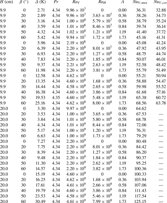
A.2. Symmetry in tilted RBC
We first consider the levelled case. The governing equations for levelled RBC satisfy the reflection symmetry about the  $y$–
$y$– $z$ plane ( $K_x$), the $x$–
$x$– $y$ plane ( $K_z$) and the rotational symmetry ( $K_{xz}=K_xK_z$) are
 \begin{gather} (T^\prime,u^\prime,v^\prime,w^\prime)(x, y, z) = K_x(T,u,v,w)(x,y,z) = (T,-u,v,w)(-x,y,z), \end{gather}
 \begin{gather}(T^\prime,u^\prime,v^\prime,w^\prime)(x, y, z) = K_z(T,u,v,w)(x,y,z) = (-T,u,v,-w)(x,y,-z), \end{gather}
 \begin{gather}(T^\prime,u^\prime,v^\prime,w^\prime)(x, y, z) = K_{xz}(T,u,v,w)(x,y,z) = (-T,-u,v,-w)(-x,y,-z). \end{gather}
 The ensemble average of the solution should also satisfy the above symmetries. In such a case, if we consider the ensemble average of horizontal Nusselt number (2.13), we have (for simplicity of discussion, the origin of the coordinates is set in the centre of the cell, therefore the boundary condition is invariant with respect to  $K_x$ transformation)
 \begin{align} 2Nu_H&\sim\left(\int_{z=-H/2}x\frac{\partial\langle T(x)\rangle}{\partial z}\, \textrm{d} S - \int_{z=H/2}x\frac{\partial\langle T(x)\rangle}{\partial z}\, \textrm{d} S\right)\nonumber\\ &\quad +\left(\int_{z=-H/2}x\frac{\partial\langle T^\prime(x)\rangle}{\partial z}\, \textrm{d} S - \int_{z=H/2}x\frac{\partial\langle T^\prime(x)\rangle}{\partial z}\, \textrm{d} S\right)\nonumber\\ &= \left(\int_{z=-H/2}x\frac{\partial\langle T(x)\rangle}{\partial z}\, \textrm{d} S - \int_{z=H/2}x\frac{\partial\langle T(x)\rangle}{\partial z}\, \textrm{d} S\right)\nonumber\\ &\quad +\left(-\int_{z=-H/2}x\frac{\partial\langle T(x)\rangle}{\partial z}\, \textrm{d} S + \int_{z=H/2}x\frac{\partial\langle T(x)\rangle}{\partial z}\, \textrm{d} S\right) = 0, \end{align}
in the above we have used the fact that  $\langle T(x)\rangle = \langle T^\prime (x)\rangle = \langle T(-x)\rangle$, and made a change of integration variable $x \rightarrow -x$ in the last step.
In the tilted case ( $\varLambda > 0$), the left–right reflection symmetry ( $K_x$) is broken, resulting in a non-zero horizontal Nusselt. Note that the $K_{xz}$ symmetry is preserved in the governing equations even in the presence of horizontal buoyancy. This means that both $T$ and $T^\prime =K_{xz}T$ are solutions of the governing equations, and so the ensemble average of temperature gradient satisfies
 \begin{equation} \left\langle\frac{\partial T(x,y,z)}{\partial z}\right\rangle = \left\langle\frac{\partial T^\prime(x,y,z)}{\partial z}\right\rangle = \left\langle\frac{\partial T(-x,y,-z)}{\partial z}\right\rangle. \end{equation}
Therefore, we can write the first term on the right-hand side of (2.13) as
 \begin{equation} \int_{z=-H/2}x\frac{\partial\langle T(x)\rangle}{\partial z}\, \textrm{d} S = \int_{z=H/2}x\frac{\partial\langle T(-x)\rangle}{\partial z}\, \textrm{d} S = \int_{z=H/2}-x\frac{\partial\langle T(x)\rangle}{\partial z}\, \textrm{d} S. \end{equation}
Again, in the last step above a change of integration variable is used. This means that the ensemble average of the two terms on the right-hand side of (2.13) are equal but with opposite sign, which leads to a non-zero  $Nu_{H}$ and which is a requirement of the $K_{xz}$ symmetry.
A.3. Experimental evaluation of the horizontal heat transfer
In the experiment, the vertical Nusselt number can be determined directly by measuring the heating power at the bottom plate and the temperature at both conducting plates (2.7). However, to determine the horizontal Nusselt number  $Nu_H$, one needs to know the exact horizontal distribution of the vertical temperature gradient, i.e. $\partial T(x,y)/\partial z$, on both plates (see (2.13)), which is difficult to obtain experimentally. In this subsection, we propose an indirect method, utilizing the measured azimuthal temperature profile at midheight, to estimate the horizontal Nusselt number $Nu_H$.
To do this, we first consider the fact that when the cold descending plumes impinge on the left-hand side of the bottom plate, the thermal boundary layer  $\delta _{T,c}$ therein becomes thinner. Whereas hot plumes aggregate on the right-hand side of the same plate, thicken the thermal boundary layer $\delta _{T,h}$ there. We approximate the ratio between the thermal boundary thicknesses at $\theta = 0$ and ${\rm \pi}$ to be
 \begin{equation} \delta_{T,h}/\delta_{T,c} = (0.5 + \tilde{T}_A)/(0.5 - \tilde{T}_A),\end{equation}
here  $\tilde {T}_A = T_A/\varDelta$ is the normalized amplitude of the LSC. In the next step, we further assume the ratio between the temperature gradients at these two points to be
 \begin{equation} \frac{(\partial \tilde{T}/\partial \tilde{z})_{\tilde{x} = 0}}{(\partial \tilde{T}/\partial \tilde{z})_{\tilde{x} = 1}} = \frac{(0.5 - \tilde{T}_A)^2}{(0.5 + \tilde{T}_A)^2}\approx\frac{1-4\tilde{T}_A}{1+4\tilde{T}_A}.\end{equation}
 Since the local heat flux is proportional to the local temperature gradient, the normalization condition requires that the integral of  $\partial \tilde {T}/\partial \tilde {z}$ over the bottom/top plate equals to $Nu_V$. Putting all these together, the local temperature gradient can be estimated as
 \begin{equation} \partial \tilde{T}/\partial \tilde{z} = [1-4\tilde{T}_{\tilde{z} = 0.5}(\tilde{x})]Nu_V.\end{equation}
 Here we have applied our second assumption that the temperature gradient depends only on the horizontal position  $\partial _{\tilde {z}}\tilde {T}/\partial \tilde {y} = 0$.
Substitute (A9) into (2.13), and integrating over both the top and bottom plates, we obtain
 \begin{align} \int_{\tilde{z} = 0}\tilde{x}\frac{\partial \tilde{T}}{\partial \tilde{z}}\, \textrm{d} \tilde{S} - \int_{\tilde{z} = 1}\tilde{x}\frac{\partial \tilde{T}}{\partial \tilde{z}}\, \textrm{d} \tilde{S} & = 4Nu_V \tilde{T}_A\int_{0}^{\rm \pi}\cos^2\theta|\cos\theta|^\zeta \sin\theta \, \textrm{d} (\cos\theta)\nonumber\\ &= \frac{{\rm \pi} Nu_V}{2}\tilde{T}_Ag(\zeta), \end{align}
where  $g(\zeta )$ is a geometrical factor that depends only on the coherency index $\zeta$, which can be determined by a definite integration as follows:
 \begin{equation} g(\zeta) = \frac{16}{(3+\zeta){\rm \pi}}\int_{0}^{1}\sqrt{1-\xi^{{2}/({3+\zeta})}}\, \textrm{d} \xi.\end{equation}
 Combining all the above together, the horizontal Nusselt number  $Nu_H$ can be expressed as
 \begin{equation} Nu_H = 2Nu_V \tilde{T}_Ag(\zeta).\end{equation}
 In (A12), the horizontal Nusselt is proportional to the vertical Nusselt  $Nu_V$. This is indeed as expected for if more heat is supplied at the bottom plate, the large-scale circulation brings more heat from the left-bottom corner to the top-right corner.
After obtaining  $\zeta$ and $\tilde {T}_A$ from the measured mean temperature profiles, we are able to estimate the horizontal Nusselt number using (A12). We plot the experimentally estimated $Nu_H$ along with our DNS data in figure 20. Quantitative agreement is only observed for intermediate buoyancy ratios. Large deviations are observed at the rightmost point. The reason for this discrepancy may be that the azimuthal profile (3.4) is not accurate for large $\varLambda$ (see figure 9) and the assumption we used in deriving the $Nu_H$ is not applicable any more at such high $\varLambda$ value. Although this indirect method seems to be applicable for a limited parameter range, we stress that to the best of our knowledge, this is not only the first attempt to experimentally quantify $Nu_H$, but it also gives the right order of magnitude.

Figure 20. Horizontal Nusselt number as a function of buoyancy ratio. The solid circles correspond to an estimation of (A12) using experimentally measured data; open triangles are from DNS.
Table 3. Simulation parameters and corresponding vertical Nusselt Nu V and horizontal Nusselt number Nu H.