







1. Introduction
Particle-laden suspensions are abundant in biological, industrial and geophysical flows such as blood flow in the human body, the food industry and pyroclastic flows from volcanoes, with most of these applications concerning turbulent flows. The presence of solid particles introduces additional momentum interactions between the particles and the fluid, which results in modulation of the flow structures and of the overall drag; see e.g. Brandt & Coletti (Reference Brandt and Coletti2022) for a recent review of the topic. Considering the typical Reynolds numbers encountered in the mentioned applications, inertia plays a significant role at the particle scale. Here, we therefore examine in detail how flow and the particle dynamics change when increasing the Reynolds number to values higher than those typically adopted in previous fully resolved simulations. The flow of particle suspensions has been the object of several previous studies, and here we present a brief review of the main findings, starting from viscous flows and increasing the significance of inertial effects.
The rheological properties of suspensions, i.e. the relation between the applied rate of strain and the resulting stress, have been often studied in the viscous Stokesian regime, where the inertial effects are negligible. The presence of particles affects the deformation of the surrounding fluid and the effective viscosity  $\mu _e$ of the particle–fluid mixture depends on the dynamics of the dispersed phase as well as the imposed shear rate. The first attempts can be traced back to Einstein (Reference Einstein1905, Reference Einstein1911), who derived an analytical linear relation for the effective viscosity of a dilute suspension (assuming negligible inter-particle interactions): $\mu _e = \mu (1+2.5\phi )$, with $\mu$ the viscosity of the fluid phase and $\phi$ the volume fraction of the dispersed phase. A quadratic correction, accounting for mutual particle interactions, was later proposed for slightly higher volume fractions (Batchelor Reference Batchelor1970; Batchelor & Green Reference Batchelor and Green1972). Only semi-empirical formulas, like those from von Eilers (Reference von Eilers1941) and Krieger & Dougherty (Reference Krieger and Dougherty1959), are, however, available for characterizing the rheology at higher concentrations.
Inertial effects, yet in the laminar regime, induce significant modifications to the suspension microstructure and create a local anisotropy responsible for shear thickening, and thus a change of the macroscopic suspension dynamics; see e.g. Kulkarni & Morris (Reference Kulkarni and Morris2008), Brown & Jaeger (Reference Brown and Jaeger2009) and Yeo & Maxey (Reference Yeo and Maxey2011). This shear-thickening behaviour can be quantitatively estimated by calculating the increase in effective volume fraction due to a region downstream of a reference particle which is devoid of any particle flux (Picano et al. Reference Picano, Breugem, Mitra and Brandt2013). The highly inertial regime was considered in the pioneering work of Bagnold (Reference Bagnold1954), who experimented with neutrally buoyant particles in a Taylor–Couette set-up at varying shear rates. At small shear rates, he observed a viscous Newtonian-like regime – shear stress varied linearly with the applied shear rate – with a viscosity corrected for the bulk particle concentration. Even at these small shear rates, a non-Newtonian behaviour was observed in the form of normal or dispersive stresses. On the other hand, at higher shear rates, Bagnold observed a particle-inertia dominated regime, where the shear stress varies quadratically with the applied shear rate (see also Hunt et al. Reference Hunt, Zenit, Campbell and Brennen2002).
Increasing the Reynolds number, the macroscopic flow behaviour changes rapidly from the laminar regime to the chaotic dynamics of transitional and turbulent flows. Matas, Morris & Guazzelli (Reference Matas, Morris and Guazzelli2003) explored the influence of neutrally buoyant spherical particles on the transition to turbulence in pipe flows. For the range of particle size tested by the authors, they observed that relatively smaller particles lead to a monotonic concentration-dependent and size-independent increase in the critical Reynolds number when transition happens; the delay in transition was explained by the increase of the effective viscosity of the suspension. However, a non-monotonic behaviour was observed for relatively larger particles: an initial decrease of the critical Reynolds number with the solid volume fraction, with a minimum which is lower for larger particles, followed by an increase when further increasing the particle concentration; see also Yu et al. (Reference Yu, Wu, Shao and Lin2013). These results were confirmed by the simulations of Loisel et al. (Reference Loisel, Abbas, Masbernat and Climent2013), who showed that modulation of the velocity fluctuations plays a major role for larger particles.
Lashgari et al. (Reference Lashgari, Picano, Breugem and Brandt2014, Reference Lashgari, Picano, Breugem and Brandt2016) confirmed the existence of three different regimes for suspension of finite-sized particulate flows when changing the volume fraction and the Reynolds number: a laminar-like regime where the viscous stress is dominant, a turbulent-like regime where the turbulent Reynolds stress plays the main role in the momentum transfer across the channel and a third regime, denoted as inertial shear thickening, characterized by a significant enhancement of the wall shear stress due to the noticeable contribution of the particle stress. The authors showed that different momentum transfer mechanisms were at play at the microscopic scale: a uniform particle distribution was observed in flows dominated by the turbulent stress and accumulation of particles in the core region for the flows dominated by the particle-induced stress. Picano, Breugem & Brandt (Reference Picano, Breugem and Brandt2015) studied dense suspensions in turbulent channel flow up to volume fraction  $\phi =0.2$. They showed that the velocity fluctuation intensities and the Reynolds shear stress gently increase with volume fraction and then sharply decrease after a local maximum, even though the overall drag still increases. They attributed the drag increase to the enhancement of turbulence activity up to a certain volume fraction and then to the particle-induced stresses, which govern the dynamics at dense conditions. Costa et al. (Reference Costa, Picano, Brandt and Breugem2016) explained that the turbulent drag of suspensions is always higher than what is predicted by only accounting for the effective viscosity of the suspension. They attributed this increase to the formation of a particle wall layer, a layer of particles forming near the wall in turbulent suspensions. Based on the thickness of the particle wall layer, they proposed a relation able to predict the friction Reynolds number as a function of the bulk Reynolds number. Note, however, that this particle wall layer almost completely disappears in the case of oblate particles, leading to a drag lower than that of the single-phase turbulent flow (Ardekani et al. Reference Ardekani, Costa, Breugem, Picano and Brandt2017).
Building on the previous studies of Lashgari et al. (Reference Lashgari, Picano, Breugem and Brandt2016) and Picano et al. (Reference Picano, Breugem and Brandt2015), the main aim of the present work is to investigate the interactions between the phases of a suspension with the emphasis on the highly inertial and dense conditions – aiming to approach the so-called Bagnoldian regime with fully resolved simulations by extending the range of volume fractions and Reynolds numbers investigated in previous studies. In particular, we will show that in dense conditions, the Reynolds shear stresses become more important than the particle-induced stresses when increasing the inertial effects, that the particles’ dynamics is highly inhomogeneous and that different mechanisms dictate the particle interactions at different distances from the walls. In other words, the simulations presented here, corroborated by recent experiments, seem to disprove the conjecture left by Bagnold (Reference Bagnold1954); i.e. ‘it seems that the residual fluid shear stress due to turbulence progressively gives place to grain shear stress’ when increasing volume fraction and Reynolds number. Our results indicate that Reynolds stresses and the associated correlated motions, characteristics of near-wall turbulence, would eventually prevail over the resistance to deformation presented by the rigid finite-size particles for volume fractions lower than 30 %.
2. Methods and computational set-up
2.1. Governing equations
We study the motion of suspended rigid neutrally buoyant particles in a Newtonian carrier fluid. The evolution of the fluid phase is described by the incompressible Navier–Stokes equations
 \begin{gather} {\boldsymbol{\nabla} \boldsymbol{\cdot} \boldsymbol{u}} = 0, \end{gather}
 \begin{gather}\frac{\partial \boldsymbol{u}}{\partial t} + {\left(\boldsymbol{u}\boldsymbol{\cdot} \boldsymbol{\nabla}\right) \boldsymbol{u}} ={-} \frac{\boldsymbol{\nabla} (p+p_e) }{\rho} + \nu \nabla^2 \boldsymbol{u} + \boldsymbol{f}, \end{gather}
where  $\rho$ is the fluid density, $\nu$ the fluid kinematic viscosity, $p$ the fluid pressure with respect to an arbitrary constant reference value and $\boldsymbol {\nabla } p_e$ the external pressure gradient that serves as the driving force for the flow. Also, $\boldsymbol {u} = (u,v,w)$ is the flow velocity, with $u$,
$u$,  $v$ and $w$ being its $x$ (streamwise), $y$ (wall-normal) and $z$ (spanwise) components. The source term on the right-hand side of (2.2), $\boldsymbol {f}$, accounts for the coupling between finite-size particles and the carrier fluid.
The Newton–Euler equations govern the motion of each spherical particle with mass  $m_p$, and moment of inertia $I_p$
$I_p$
 \begin{gather} m_p \frac{\mathrm{d} \boldsymbol{u}_p}{\mathrm{d} t} = \oint_{\partial \varOmega_p} \boldsymbol{\tau} \boldsymbol{\cdot} \boldsymbol {n} \,\mathrm{d}A + \boldsymbol{F}_{col}, \end{gather}
 \begin{gather}I_p\frac{\mathrm{d} \boldsymbol{\omega}_p}{\mathrm{d}t} = \oint_{\partial \varOmega_p} \boldsymbol{r} \times (\boldsymbol{\tau} \boldsymbol{\cdot} \boldsymbol {n}) \,\mathrm{d}A + \boldsymbol{T}_{col}, \end{gather}
where here,  $\boldsymbol {u}_p$ and $\boldsymbol {\omega }_p$ denote the particle linear and angular velocity vectors, $\boldsymbol {r}$ the position vector with respect to the particle centre and $\boldsymbol {n}$ the outward-pointing unit normal to the particle surface $\partial \varOmega _p$. The fluid stress tensor is given by $\boldsymbol {\tau } = -(p+p_e) \boldsymbol {I} + \rho \nu (\boldsymbol {\nabla } \boldsymbol {u} + \boldsymbol {\nabla } \boldsymbol {u}^T)$, and $\boldsymbol {F}_{col}$ and $\boldsymbol {T}_{col}$ denote the force and torque resulting from short-range particle–particle or particle–wall interactions, such as lubrication and solid contact.
Equations ((2.1)–(2.4)) are coupled through the no-slip and no-penetration conditions at the particle surface
 \begin{equation} \boldsymbol{u}|_{\partial \varOmega_p} = \boldsymbol{u}_p + \boldsymbol{\omega}_p \times \boldsymbol{r}.\end{equation}
2.2. Numerical method
The governing equations are solved by a Navier–Stokes solver coupled with an immersed boundary method (IBM) for interphase coupling. The direct forcing IBM used here is the one initially proposed by Uhlmann (Reference Uhlmann2005) and extended by Breugem (Reference Breugem2012) to fully resolve fluid–solid interactions with second-order convergence for several integral observables. The method has been used extensively with several validations; see e.g. Picano et al. (Reference Picano, Breugem and Brandt2015), Lashgari et al. (Reference Lashgari, Picano, Breugem and Brandt2016), de Motta et al. (Reference de Motta2019), Yousefi, Ardekani & Brandt (Reference Yousefi, Ardekani and Brandt2020) and Yousefi et al. (Reference Yousefi, Ardekani, Picano and Brandt2021). The method and implementation details have been carefully presented in these references. Below, we only present a brief description of the method, for the sake of completeness.
The Navier–Stokes equations are solved on a fixed Eulerian mesh, while the spherical particles are discretized by a set of moving Lagrangian points, uniformly distributed on their surface. The coupling between these two phases is achieved by the IBM forcing in three steps: (i) the fluid prediction velocity is interpolated from the Eulerian to the Lagrangian grid, (ii) the IBM force is calculated from the difference between the interpolated local fluid velocity and the local particle velocity on each Lagrangian grid point and (iii) the resulting IBM force is spread from the Lagrangian to the Eulerian grid points. The method uses the regularized Dirac delta function of Roma, Peskin & Berger (Reference Roma, Peskin and Berger1999) to perform interpolation and spreading operations, with the support of three grid cells along each direction.
When the distance between particles or with a wall becomes smaller than the grid spacing, an additional lubrication correction, which also accounts for surface roughness effects at very close proximity, is added to capture the correct particle dynamics. Finally, when the particles are in contact, the lubrication force is switched off and a soft-sphere collision model is activated to model collisions/contacts from the relative velocity and (slight) overlap of colliding particles. Here, the particles have been considered to be frictionless, with a normal dry coefficient of restitution of  $0.97$, which is typical value for hard materials such as glass or steel spheres; see Foerster et al. (Reference Foerster, Louge, Chang and Allia1994). These collision parameters may become dynamically significant for denser cases, where sustained solid–solid contacts are frequent and the mediation of the collisional dynamics by short-range hydrodynamic interactions becomes less important. Nevertheless, we decided to use frictionless, nearly perfectly elastic spheres to keep the number of governing parameters small. More details on the short-range models and corresponding validations can be found in Costa et al. (Reference Costa, Boersma, Westerweel and Breugem2015).
The numerical method was implemented in a parallel framework for simulations on many CPUs, using a pencil domain decomposition for the flow, and a leader-workers strategy for the particles, as described in Costa (Reference Costa2017).
2.3. Computational set-up
In the present work, we investigate the channel flow between two parallel walls, laden with rigid spherical particles. The size of the computational domain is  $L_x=6h$, $L_y=2h$ and $L_z=3h$ in the streamwise, wall-normal and spanwise directions, where $h$ is half the distance between the channel walls. The flow is periodic in the streamwise and spanwise directions, with no-slip and no-penetration boundary conditions imposed at the bottom and top walls. The flow is forced by a uniform pressure gradient which ensures a constant bulk velocity, $U_b$. The flow dynamics is governed by three parameters: the Reynolds number $Re \equiv U_b (2h)/ \nu$, the particle size ratio $D_p/h$ and the bulk volume fraction of solid neutrally buoyant particles $\phi = N_pV_p/V_t$, where $U_b$ is the flow bulk velocity, $D_p$ the particle diameter, $N_p$ the total number of particles and $V_p$ and $V_t$ the volumes of a particle and of the computational domain. The particle size ratio is $D_p/h=1/7.5$ for all cases, while the Reynolds number varies in the range $3000 \leq Re \leq 15\ 000$ (by changing the viscosity), and the particle volume fraction $0 \leq \phi \leq 0.3$. The number of particles for the highest volume fraction, $\phi =0.3$, is $8702$.
Since the Reynolds number spans over a large range, we use three different grid resolutions to secure the resolution for all cases. The parameters pertaining to the grid resolution are summarized in table 1.
Table 1. Computational parameters for different values of the Reynolds number. Here,  ${\rm \Delta} x$ denotes the Eulerian grid spacing, $N_x$, $N_y$ and $N_z$ the number of Eulerian grid points in the $x$,
$x$,  $y$ and $z$ coordinate directions, $N_L$ number of Lagrangian grid points on the surface of each particle and ${\rm \Delta} x^+ \equiv u_{\tau } {\rm \Delta} x / \nu$ the Eulerian grid spacing in inner-scale units.

3. Results
We start by reporting the mean wall shear stress,  $\tau _w$, expressed in terms of a friction factor, $f = 2\tau _w / (\rho U_b^2)$, for the different cases. Figure 1(a) shows $f$ as a function of the Reynolds number for different particle volume fractions. For most cases, consistently with previous observations, the friction factor increases with increasing volume fraction. Interestingly, this trend is not observed at lower Reynolds numbers, with the case with $\phi =0.2$ showing a lower value of $f$ than for $\phi =0.1$. Adding the suspended phase alters the rheological properties of the suspension, which can be quantified using the relative viscosity $\nu _r$, i.e. the ratio between the effective viscosity of the suspension and the viscosity of the fluid phase $\nu _r=\nu _e/\nu$. Figure 1(b) shows therefore the same data vs the Reynolds number based on effective viscosity, $Re_e = Re / \nu _r$. The increased effective viscosity $\nu _e$ is obtained by the semi-empirical fit from von Eilers (Reference von Eilers1941)
 \begin{equation} \nu_r = \frac{\nu_e}{\nu} = \left( 1+ \frac{5\phi}{4(1-\phi/\phi_{max})} \right)^2,\end{equation}
with  $\phi _{max} = 0.65$, corresponding to the volume fraction at random close packing. Comparing the laden cases with the single-phase ones, we observe that for the range of parameters considered here, the friction factor collapses relatively well to values larger than the single-phase ones when displayed vs the normalized Reynolds number, $Re_e = Re / \nu _r$. In the figure, we also report the experimental data of Zade (Reference Zade2019), indicated by stars, for pipe flow with similar relative particle size (the pipe to particle diameter ratio is equal to $16$) and even larger values of the Reynolds number. The data show that, at higher $Re$, the friction factor of the multiphase cases approaches the single-phase one and goes even below it for the largest Reynolds numbers considered. This behaviour, consistent with the trend from the present simulations, suggests that, although an effective-viscosity description is not sufficient to estimate the drag in the suspension at intermediate values of the Reynolds number, it becomes relevant again at higher inertia. Similar results are obtained from the experiments in Agrawal (Reference Agrawal2021), where the pressure drops in particle suspensions are also investigated in high Reynolds number pipe flow.

Figure 1. Friction factor,  $f=\tau _w / (0.5\rho U_b^2)$, vs (a) the Reynolds number and (b) the Reynolds number based on effective viscosity, $Re_e = Re / \nu _r$; the star symbols represent experimental data of Zade (Reference Zade2019) in pipe flow with the size ratio between the pipe to particle diameter equal to $16$. (c) Friction Reynolds number $Re_{\tau }= u_{\tau } h /\nu$ and turbulent friction Reynolds number $Re_{\tau }^T = u_{\tau }^T h /\nu$ vs the bulk volume fraction $\phi$. (d) Effective viscosity, $\nu _e$, vs Bagnold number for different values of $\phi$; the inset reports the Bagnold number as a function of the Reynolds number.
Figure 1(c) reports the friction Reynolds number  $Re_{\tau } \equiv u_{\tau }h/\nu$ as an indication of the total drag, together with the turbulent friction Reynolds number $Re_{\tau }^T \equiv u_{\tau }^T h/\nu$ to quantify the level of turbulence activity, where $u_{\tau } \equiv \sqrt {\tau _w /\rho }$ is the friction velocity and $u_{\tau }^T \equiv \sqrt {{\rm d}\langle u^{\prime } v^{\prime } \rangle /{{\rm d} y}}|_{y=h}$ (i.e. the square root of the wall-normal derivative of the Reynolds stress profile at the channel centreline; see e.g. Pope Reference Pope2000). The values of the two Reynolds numbers are close in the unladen cases, $\phi =0$, as expected. Increasing the volume fraction, $Re_{\tau }$ increases monotonically, while $Re_{\tau }^T$ has a non-monotonic behaviour: increasing with $\phi$ (at a slower rate compared with $Re_{\tau }$) up to a certain point and then decreasing, further increasing the volume fraction. All the investigated cases show a significant decrease of $Re_{\tau }^T$ at $\phi =0.3$; in § 3.1, we will assess the predictions of the turbulent activity from $Re_{\tau }^T$ by considering the contribution of the Reynolds shear stresses to the streamwise momentum budget and showing how this measure may mask the complete dynamics in multiphase flows where addition of a dispersed phase differently modulates the near-wall and centreline dynamics.
To study inertial suspensions, Bagnold (Reference Bagnold1954) introduced the parameter known as the Bagnold number,  $Ba = 4 Re_p \sqrt {\lambda }$, where $\lambda = 1 / ((0.74 / \phi )^{1/3} - 1)$ denotes the ratio between the particle diameter and the average radial separation distance, and $Re_p = \dot {\gamma } D_p^2 / 4 \nu$, the particle Reynolds number with $\dot {\gamma } = U_b /h$ the average shear rate across the channel. This non-dimensional number can be interpreted as the ratio between collisional and viscous stresses. Values $Ba < 40$ define a macro-viscous regime, where the relation between the stress and shear rate is linear while $Ba > 450$ the Bagnoldian regime, which is characterized by a quadratic dependence of the stress on the shear rate. Figure 1(d) shows the effective viscosity as a function of the Bagnold number for different volume fractions, while the inset reports the Bagnold number as a function of the Reynolds number. The effective viscosity is calculated as the viscosity of a single-phase laminar flow that would give the same shear stress as in our simulations
 \begin{equation} \nu_e = \tau_{xy} \left/ \left(\rho \left.\frac{{\rm d}U}{{\rm d} y} \right|_{lam. \, \phi=0\,\%}\right) \right., \end{equation}
with  $\tau _{xy}$ the shear stress in the streamwise direction. The data follow a power law, $\nu _e \propto Ba^a$, with exponent $0 < a <1$, indicating a departure from the macro-viscous regime, but not yet the fully Bagnoldian regime, where $\nu _e$ is proportional to $Ba$, hence the quadratic relation of stress with the shear rate. The exponent $a$ is closer to unity for the cases with higher Bagnold number.
Next, we examine the single-point statistics from the simulation data. The profiles of averaged Eulerian statistics reported here correspond to mean intrinsic averages. The intrinsic average of a quantity  $\xi$ is computed as
 \begin{equation} \langle \xi\rangle(y_j) = \frac{\displaystyle \sum_{ik,t}\xi_{ijk,t}\varPsi_{ijk,t}}{\displaystyle \sum_{ik,t}\varPsi_{ijk,t}}, \quad \langle \xi_p\rangle(y_j) = \frac{\displaystyle \sum_{ik,t}\xi_{ijk,t}(1 - \varPsi_{ijk,t})}{\displaystyle \sum_{ik,t}(1 - \varPsi_{ijk,t})} , \end{equation}
where  $\varPsi _{ijk,t}$ is the fluid volume fraction at the grid cell $ijk$ and instant $t$, and $y_j$ the wall-normal location of the averaging bin, which extends over the entire domain in the two homogeneous directions. Figure 2 shows the mean streamwise fluid velocity profiles for different values of the particle volume fraction. We observe two distinct trends in regions close to the channel wall ( $y/h < 0.3$) and close to the channel centreline ( $y/h > 0.7$): close to the wall, the mean flow decreases (increases) with increasing $\phi$ ( $Re$), while at the core of the channel we observe the opposite behaviour, i.e. blunter and turbulent-like profiles with decreasing (increasing) $\phi$ ( $Re$) (we recall that the flow rate is constant in these simulations). The profiles show a progressive decrease in slope near the wall with increasing $\phi$ and an increase in the centreline velocity, which are symptoms of turbulence attenuation (Zade et al. Reference Zade, Costa, Fornari, Lundell and Brandt2018).
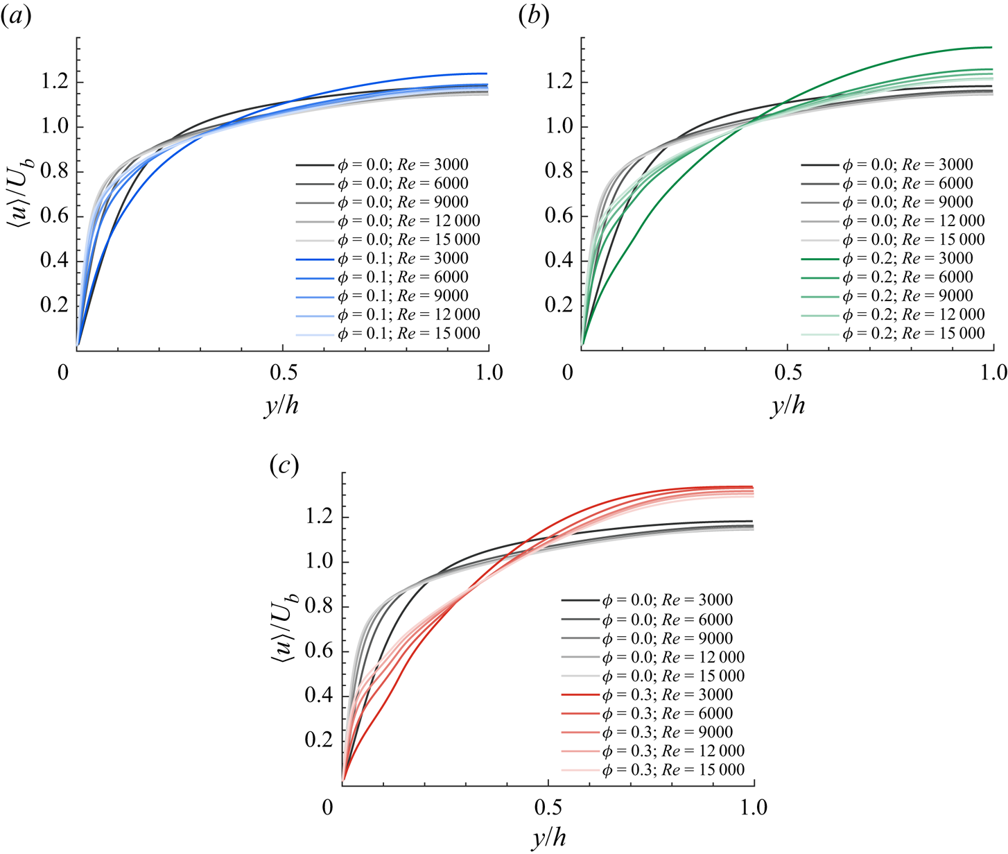
Figure 2. Outer-scaled mean fluid velocity profiles, compared with the single-phase data, for (a)  $\phi =0.1$, (b) $\phi =0.2$ and (c) $\phi =0.3$.
The root-mean-square (r.m.s.) of the fluid velocity fluctuations and the Reynolds shear stress are reported in figure 3 in outer units. We note that, in line with previous studies (see e.g. Picano et al. (Reference Picano, Breugem and Brandt2015) and Shao, Wu & Yu (Reference Shao, Wu and Yu2012)), the peak of the streamwise velocity r.m.s.,  $u^{rms}$, decreases monotonically for increasing $\phi$. For the cross-stream components, instead, we observe a non-monotonic behaviour when increasing $\phi$ (see figure 3b,c): at $\phi =0.1$ the peak of $v^{rms}$ and $w^{rms}$ profiles are higher compared with the single-phase ones, while for $\phi \geq 0.2$, the peaks drop to values slightly lower than the single-phase flow. The profiles of the Reynolds stresses, which represent the main mechanism for production of turbulent fluctuations, are depicted in figure 3(d). While these stresses increase for $\phi =0.1$, they decrease substantially for $\phi \geq 0.2$ compared with the single-phase flow, indicating that although the presence of particle at $\phi =0.1$ is able to amplify the fluid fluctuations, the turbulence level decreases significantly at higher volume fractions, to a point that we have a re-laminarized flow for low values of $Re$ at the bulk of the channel. It is also worth noting that, on increasing the Reynolds number, the difference between the profiles of the laden cases and the single-phase flow with the same $Re$ decreases significantly, which is in line with the numerical results of Yu et al. (Reference Yu, Zhu, Wang and Shao2019) in turbulent channel flow, laden with finite-size particles at $Re_{\tau }=395$.

Figure 3. Wall-normal profiles of (a) streamwise, (b) wall-normal and (c) spanwise fluid velocity r.m.s. (d) Wall-normal profiles of the Reynolds stress. All panels are in outer scale.
The wall-normal profiles of the local particle volume fraction,  $\varPhi (y)$, are depicted in figure 4(a) for different Reynolds numbers and bulk particle volume fractions. At $\phi =0.1$, we observe an almost uniform distribution of the particles across the channel walls, except for the region $y/h < D_p$, close to the wall, where the kinematic constrain on the particle motion results in the formation of a layer (Picano et al. Reference Picano, Breugem and Brandt2015). In this case, turbulent mixing induces a homogeneous solid concentration in the bulk, whereas particles experience asymmetric interaction of the lubrication force with the wall, which hinders particles in that region. The presence of a particle wall layer is associated with an increase in drag (see Costa et al. (Reference Costa, Picano, Brandt and Breugem2016) and Costa et al. (Reference Costa, Picano, Brandt and Breugem2018)), while the role of the rotation for the layer formation is discussed in Peng, Ayala & Wang (Reference Peng, Ayala and Wang2019). Increasing the volume fraction to $\phi =0.2$, the peak in the profiles close to the wall becomes more distinct.

Figure 4. (a) Profiles of the local solid volume fraction as a function of the wall-normal distance. (b) Outer-scaled mean streamwise particle velocity profiles; the inset shows the apparent particle-to-fluid slip velocity,  $\langle u_p \rangle - \langle u \rangle$, in semi-logarithmic scale, while the vertical dashed line indicates the wall-normal distance corresponding to one particle diameter.
The concentration profiles also change with the Reynolds number: at  $Re=3000$, we observe a weak migration of particles toward the channel centreline even at $\phi =0.2$. This is reminiscent of the Segre–Silberberg effect (Segre & Silberberg Reference Segre and Silberberg1961), an inertial effect resulting from the balance between the Saffman lift (Saffman Reference Saffman1965), inhomogeneous shear rate and wall effects; see also Yeo & Maxey (Reference Yeo and Maxey2010). Increasing $Re$, the peak close to the wall increases, the profiles become blunter and migration to the channel core attenuates; this is in contrast with previous results for a lower range of Reynolds numbers; see e.g. Yousefi et al. (Reference Yousefi, Ardekani, Picano and Brandt2021), where results are presented for $500 \leq Re \leq 5600$. At $\phi =0.3$, both the accumulation of particles in the particle wall layer and the migration towards the centreline are more significant when compared with the lower volume fraction data. In these cases also, the increase of $Re$ results in a larger peak close to the wall and less migration to the centreline, as observed for $\phi =0.2$.
Figure 4(b) shows the wall-normal profiles of the mean particle velocity for all the multiphase cases. The particle phase velocity presents a similar behaviour to the fluid phase, i.e. close to the wall the mean velocity decreases when increasing the volume fraction and increases when increasing the Reynolds number, whereas close to the channel centreline the scenario is the opposite. In line with previous observations, it is also noticeable that, close to the wall,  $y/h \leq D_p$, the particles have a mean velocity larger than that of the surrounding fluid, resulting in a significant apparent slip velocity (see inset of figure 4b). It should be considered here that, while the velocity at the wall is zero for the fluid, this is not the case for the solid phase as particles can have a relative tangential motion.
3.1. Total stress balance
The understanding of the momentum exchange between the two phases in dense particle-laden turbulent channel flow is addressed by examining the mean streamwise momentum budget. Following the rationale on the mean momentum balance given in Marchioro, Tanksley & Prosperetti (Reference Marchioro, Tanksley and Prosperetti1999) and Picano et al. (Reference Picano, Breugem and Brandt2015), the three contributions to the total stress,  $\tau$, in a plane channel are the viscous stress $\tau _V$, the Reynolds stress $\tau _T$ (due to the correlated motions of fluid and particles) and the particle stress $\tau _P$ (due to the particle resistance to deformation, the stresslet and particle–particle interactions/collisions)
 \begin{equation} \tau (y) = \tau_V + \tau_T + \tau_P = \rho u_{\tau}^2(1-y),\end{equation}
where
 \begin{gather} \tau_V = \rho\nu (1-\varPhi) \frac{{\rm d} U}{{\rm d} y} , \end{gather}
 \begin{gather}\tau_T ={-}\rho(1-\varPhi) \langle u^{\prime} v^{\prime} \rangle - \varPhi \langle u_p^{\prime} v_p^{\prime} \rangle , \end{gather}
 \begin{gather}\tau_P = \varPhi \langle \sigma^p_{xy} \rangle , \end{gather}
and  $\sigma ^p_{xy}$ is the general stress in the particle phase, projected in the streamwise direction.
Figure 5 reports the stress balance given in (3.4) for each bulk volume fraction in panels (a–d); the results are normalized by the corresponding mean wall shear,  $\rho u_{\tau }^2$. Examining the single-phase cases (figure 5a), we observe the classical results where the total stress $\tau$, is mainly due to the turbulent Reynolds stress term for $y/h \geq 0.2$, while viscous transport dominates near the wall where fluctuations decay to zero. Increasing the Reynolds number, the place where the leading contribution to the total stress changes from $\tau _T$ to $\tau _V$ moves closer to the wall, i.e. the viscous sublayer becomes thinner.
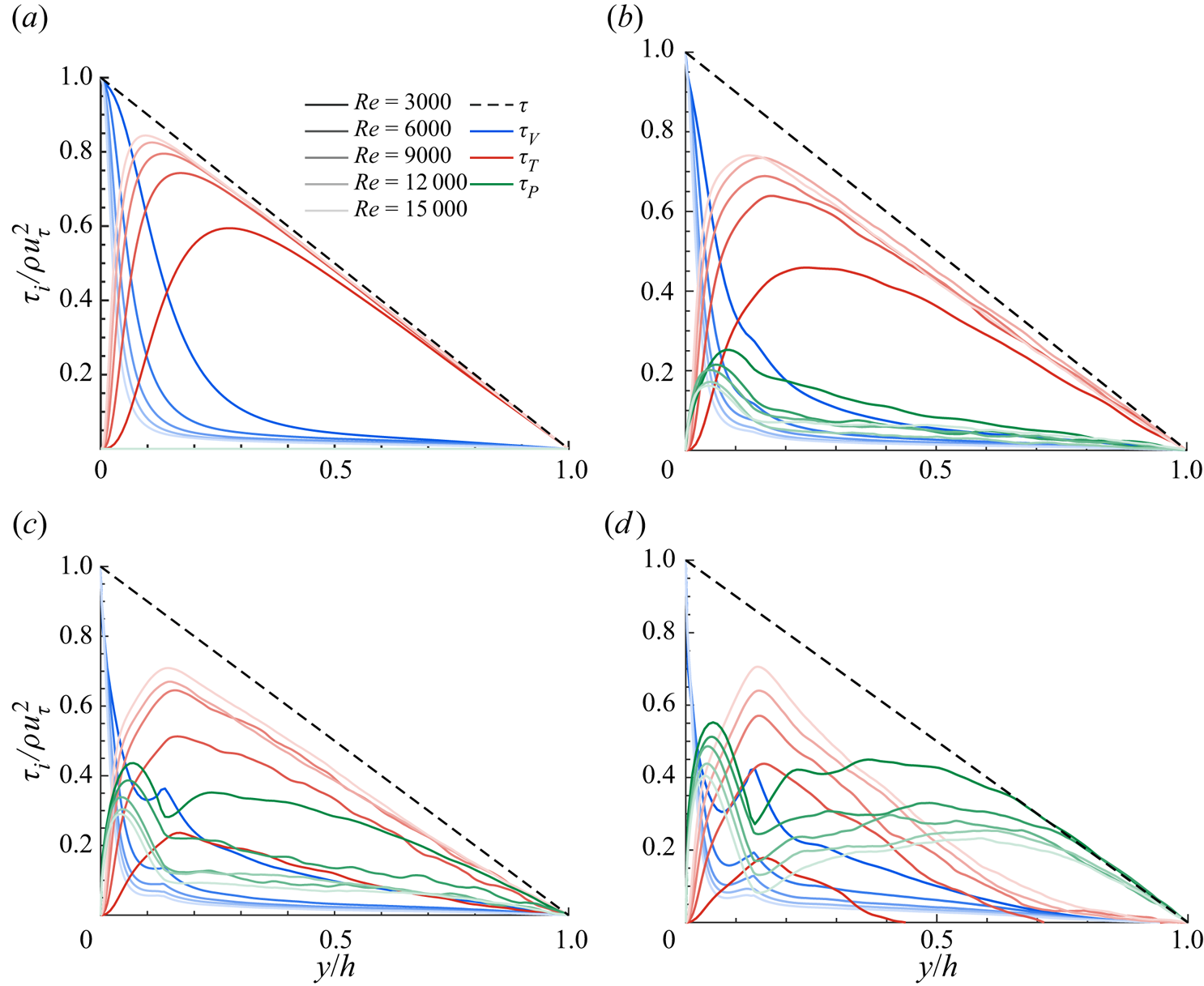
Figure 5. Momentum budget for the different bulk volume fractions: (a) single phase, (b)  $\phi =0.1$, (c) $\phi =0.2$ and (d) $\phi =0.3$. Here, $\tau$ is the total stress, $\tau _V$ denotes viscous stress, $\tau _T$ the turbulent Reynolds shear stress of the combined phase and $\tau _P$ the particle-induced stress.
At  $\phi =0.1$ (see figure 5b), the basic picture remains unaltered with the particle-induced stress $\tau _P$ showing a non-negligible contribution only near the wall, reaching a maximum at $y \approx D_p/2$. Increasing the volume fraction to $\phi =0.2$ (see figure 5c), the contribution from the particle stress becomes significant throughout the channel, although still weaker than that from the Reynolds stress, especially at higher Reynolds numbers. The near-wall peaks of the particle stress profiles are more evident at $\phi =0.2$ than $\phi =0.1$, followed by a local minimum at $y \approx 2D_p$. The local minimum of the particle stress is compensated by a local maximum of the viscous stress which is caused by the strong shear that the first layer of particles (local maximum in figure 4), flowing with significant slip velocity, imposes on the fluid above it (Costa et al. Reference Costa, Picano, Brandt and Breugem2018).
To conclude with the highest volume fraction considered,  $\phi =0.3$ (see figure 5d), we note that the dynamics is now dominated by the particle-induced stresses, as these are the major contributors to the total stress throughout the whole channel, except for the region at $0.1 \leq y/h \leq 0.3$. Close to the wall, the maximum of the profiles is larger compared with lower volume fractions and at the core ( $y/h>0.8$) almost all the stress originates from the particle-induced one. At this bulk volume fraction, the effect of the Reynolds number is more noticeable in the region $0.2 \leq y/h \leq 0.8$, where increasing $Re$ results in the increase of $\tau _T$ and the decrease of $\tau _P$, which is contrary to the observations in Lashgari et al. (Reference Lashgari, Picano, Breugem and Brandt2014) for the case of bigger particles than in the present study.
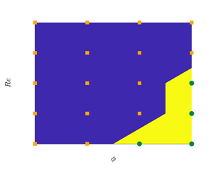
To better understand the role of the different transport mechanisms on the bulk flow behaviour in the range of Reynolds numbers and particle volume fractions investigated, we show in figure 6(a–c) contour maps of the relative contribution of viscous, Reynolds and particle stress to the total momentum transfer integrated across the channel. The contribution of the viscous stress  $\varSigma \tau _V$ is, expectedly, maximum for the lowest value of the Reynolds number, although it never becomes the dominant term (the maximum contribution in our data set is $0.34$ for the single-phase case with $Re=3000$). The numerical results of Yousefi et al. (Reference Yousefi, Ardekani, Picano and Brandt2021) with the same particle size showed that the region in the $Re-\phi$ plane for which $\varSigma \tau _V$ is the leading contributor (more than $50\,\%$ of the total stress) is limited to $Re \leq 2500$ and $\phi \leq 0.15$. The contour lines in figure 6(b) show a monotonic decrease of the contribution $\varSigma \tau _T$ when increasing $\phi$, in the fully turbulent regime. The contribution of the Reynolds stress is more than $50\,\%$ of the total for $Re > 4000$ and $\phi \leq 0.15$: the fluid and particle phases induce strong fluctuations that cannot be damped by viscous dissipation. The region with $\phi > 0.25$ and $Re < 10\ 000$ is characterized by values of the particle stress larger than $50\,\%$ of the total stress. In this region, we expect a high level of hydrodynamic and particle–particle interactions that induce strong particle stresses (see figure 6c). Increasing the Reynolds number at the highest volume fraction considered, $\phi =0.3$, the Reynolds stress term becomes the dominant contributor once again, which is in contrast with the predictions from $Re_{\tau }^T$ presented earlier in the text. This can be explained by the fact that the slope at the centreline is no longer indicative of the turbulence activity as the flow and particle dynamics are substantially different in the near-wall and core region for a suspension flow, see discussion in § 3.2. To conclude this part, we present in figure 6(d) the map of the flow regimes pertaining the present simulation data. In this map, the regions on the $Re-\phi$ plane where more than $50\,\%$ of the total momentum transfer is due to $\varSigma \tau _T$ are coloured with blue, whereas yellow indicates when more than half of the total is due to $\varSigma \tau _P$. The simulation data points are represented with orange and green symbols on the map.
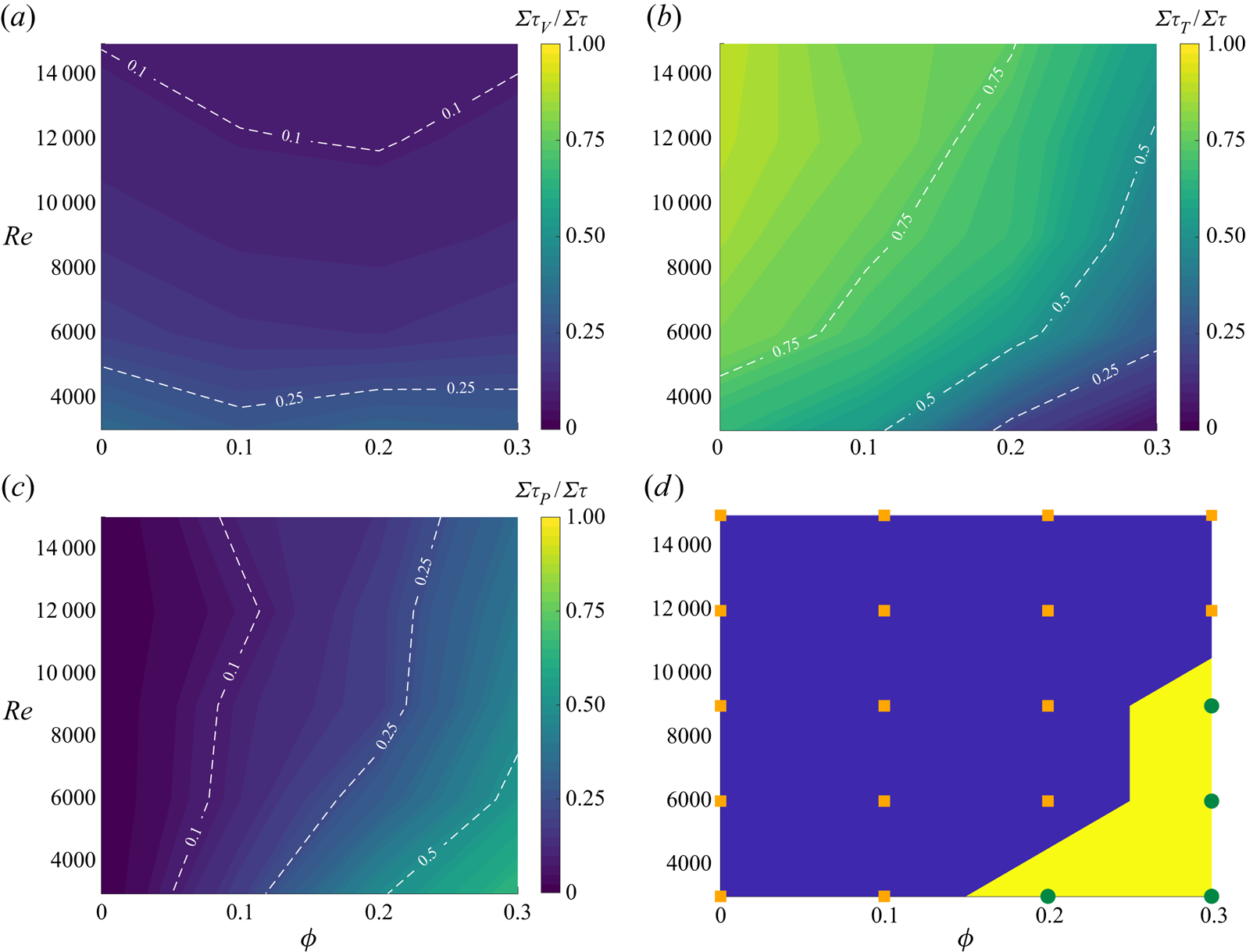
Figure 6. Contour map of the contribution of (a) viscous stress  $\varSigma \tau _V$, (b) Reynolds stress $\varSigma \tau _T$ and (c) particle-induced stress $\varSigma \tau _P$ to the total momentum transport integrated across the channel; the white dashed lines denote iso-levels as guide for the eye. Panel (d) displays a map of the flow regimes in the Reynolds number–volume fraction plane, identified by the dominant contribution to the momentum budget. Blue colour: turbulent Reynolds stress dominated regime; yellow: particle stress dominated regime. The different symbols display the available simulation data.
To provide further insight into the flow dynamics, figure 7 depicts the effect of the changes in the contribution of each term in (3.4) to the drag modulation of the multi-phase flows, compared with the single-phase references. Panel (a) shows the results at the lowest investigated Reynolds number ( $Re=3000$) and panel (b) the maximum ( $Re=15\ 000$), while panel (c) depicts an intermediate Reynolds number of $9000$; each contribution is integrated across the channel walls and normalized by the total stress of the single-phase flow with the same Reynolds number; note that all the multi-phase cases show drag increase when compared with the single-phase case. For the flows with $Re=3000$ (figure 7a), the maximum increase is $54\,\%$ at $\phi =0.3$ whereas it is $64\,\%$ for the cases at $Re=15\ 000$, also found at the highest volume fraction under consideration ( $\phi =0.3$). One should also note that, when the results for all the cases are normalized by the same value e.g. the drag of the laminar flow at $Re=3000$, the flow with $Re=15\ 000$ and $\phi =0.3$ shows a much higher drag increase compared with the one with $Re=3000$ and $\phi =0.3$ ( $\varSigma \tau |_{Re=15\ 000; \phi =0.3} / \varSigma \tau |_{Re=3000; \phi =0.3} \approx 18.3$). At the intermediate Reynolds number of $9000$, the behaviour is similar to the high $Re$ case at low volume fraction $\phi =0.1$ and to low $Re$ at high volume fraction of $\phi =0.3$.

Figure 7. The contribution of the viscous,  $\varSigma \tau _V$, Reynolds, $\varSigma \tau _T$, and particle-induced stress, $\varSigma \tau _P$, for different solid volume fractions at (a) $Re=3000$, (b) $Re=15\ 000$ and (c) $Re=9000$. Each contribution is integrated across the channel and normalized by the total stress of the single-phase flow with the same bulk Reynolds number.
Comparing the single contributions in the figure, the total absolute contribution of the viscous stress is almost unaltered, while the share of the particle-induced stress increases monotonically when increasing the volume fraction. The Reynolds stress contribution, however, shows a non-monotonic behaviour, when increasing  $\phi$ at $Re=3000$ (panel a): at $\phi =0.1$ it increases compared with the single-phase case (turbulence is enhanced), while it decreases further on increasing the volume fraction until it becomes the smallest term at $\phi =0.3$, which can be explained by the formation of a densely packed core region due to inertial particle migration (see figure 4 and Fornari et al. Reference Fornari, Formenti, Picano and Brandt2016). Indeed, in the local volume fraction profiles of figure 4, the mass fraction in the bulk is not far from the maximum value for random loose packing for all cases with $\phi =0.3$. This exacerbates the decrease in Reynolds shear stresses in the bulk. On the other hand, at $Re=15\ 000$ (figure 7b), the contribution of $\tau _T$ is enhanced with respect to the single-phase case for all the laden cases, with a peak contribution at $\phi =0.2$. The decrease for $\phi =0.3$ compared with $0.2$ is, however, not as significant as at $Re=3000$. Similarly, the monotonic increase of the importance of the particle stresses with the volume fraction is less important at the highest Reynolds number considered. These observations suggest that turbulence remains important at high Reynolds number for all volume fractions; the turbulence-induced mixing reduces the particle migration and hence the total contribution of the particle stresses. Combining the two effects, the total drag is found to approach the single-phase values when increasing the Reynolds number, which is in agreement with the experimental data discussed above.
To conclude the analysis, we show in figure 8 the terms in (3.4), normalized by the total stress in the laminar single-phase flow, as a function of  $Re$. To better follow how the picture changes when increasing the Reynolds number, we have also included data pertaining $Re \in [500\unicode{x2013}2000]$ from the numerical study of Yousefi et al. (Reference Yousefi, Ardekani, Picano and Brandt2021) with the same flow set-up and particle size. Figure 8(a) shows that the viscous stress $\tau _V$ scales almost linearly with $Re$, even though increasing $Re$ translates to decreasing viscosity in our simulations. The turbulent stress (figure 8b), starts from negligible values in the laminar regime and becomes $\propto Re^2$ after the transition, which is consistent with the mixing-length hypothesis, stating $\langle u^{\prime }v^{\prime } \rangle = l_m^2 ({\rm d}U/{{\rm d} y})^2$, with $l_m$ the mixing length. One can also note that the transition is sharper and happens at lower Reynolds number for lower volume fractions, see also Matas et al. (Reference Matas, Morris and Guazzelli2003). The particle-induced stress, on the other hand (see figure 8c), is initially proportional to $Re$ in the laminar regime, with magnitude proportional to the bulk volume fraction. Further increasing the Reynolds number, the scaling changes to $\tau _P \propto Re^{1.4}$ for the cases with the highest $Ba$ (this line is not shown in the figure). To further clarify, we present in figure 8(d) the total stress, $\tau = (\tau _V + \tau _T + \tau _P)$, as a function of $Re$. At low $Re$, where the viscous stress is dominant in the laminar-like suspension regime, with the particle-induced stress in the inertial shear-thickening regime, the total stress scales as $\propto Re$; note that the inertial shear thickening is still viscous dominated for particle Reynolds numbers lower than 10 (Alghalibi et al. Reference Alghalibi, Lashgari, Brandt and Hormozi2018). Further increasing the Reynolds number, the total stress scaling lies between two limits: for single-phase and low volume fraction cases $\tau \propto Re^{1.76}$, as suggested by the empirical fit from single-phase turbulence $Re_{\tau } \approx 0.09 Re^{0.88}$ (Pope Reference Pope2000); at higher volume fractions, the total stress should approach a quadratic dependence, $\tau \propto Re^2$, i.e. for the simulations with higher $Ba$, the stresses are closer to the quadratic scaling.
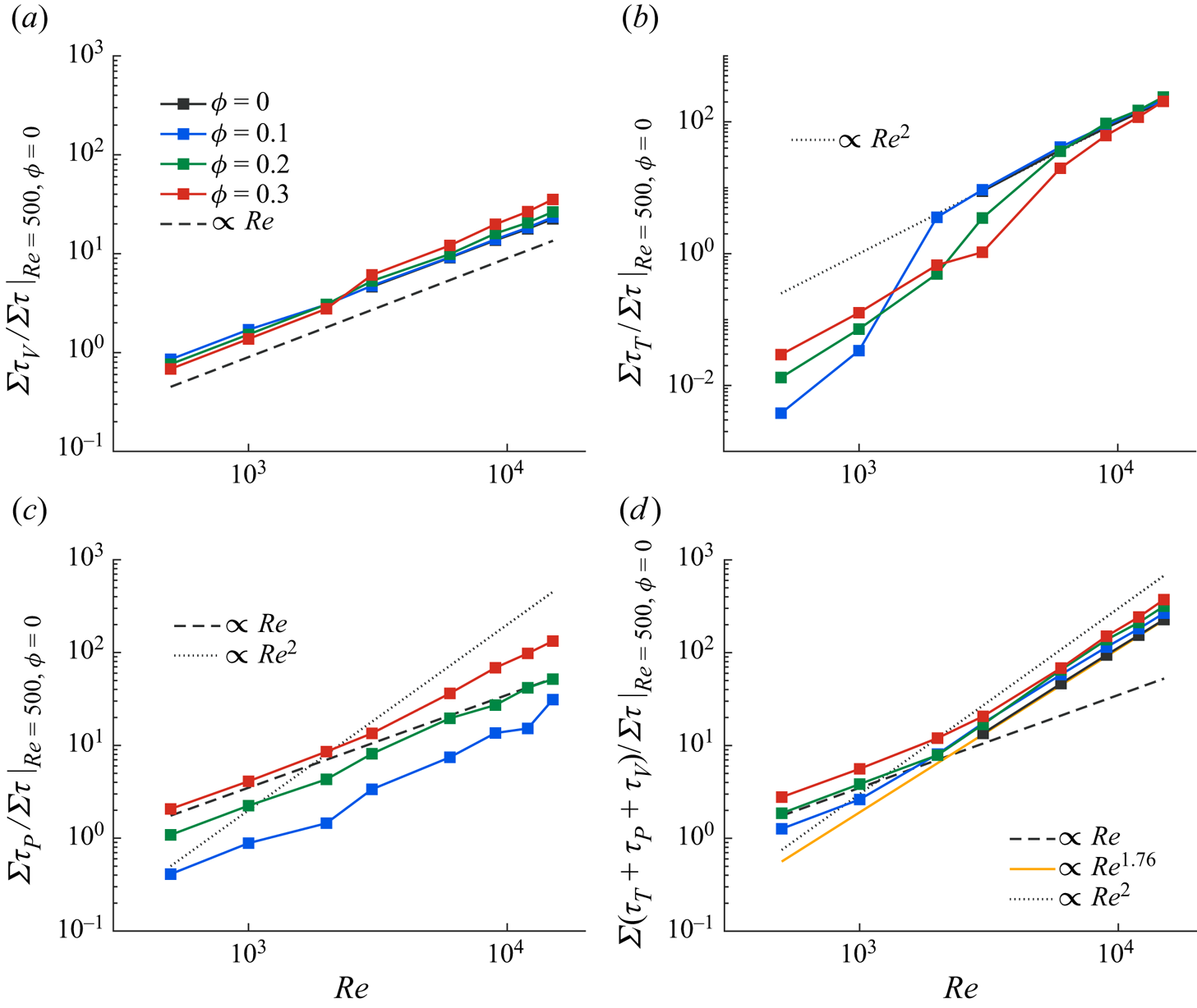
Figure 8. (a) The viscous stress,  $\varSigma \tau _V$, (b) the turbulent stress, $\varSigma \tau _T$, (c) the particle-induced stress, $\varSigma \tau _P$, and (d) the total stress, $\varSigma (\tau _V + \tau _T + \tau _P)$, normalized by the total stress in the laminar single-phase flow, as a function of the Reynolds number; the data pertaining to $Re \in [500\unicode{x2013}2000]$ are adapted from Yousefi et al. (Reference Yousefi, Ardekani, Picano and Brandt2021).
To interpret this observation, we first note that the empirical exponent  $1.76$ is found from single-phase simulations and experiments at moderately large Reynolds number, yet far from the asymptotic limit of Prandtl theory, and is within the viscous linear and the turbulent quadratic behaviours. In particle-laden flows, we have the additional contribution from the particle stress, which tends to scale as $\propto Re^{1.4}$ at the highest Reynolds number considered here, and should approach a quadratic dependence in the Bagnoldian regime. It is therefore not surprising that at these high Reynolds numbers one sees something closer to the quadratic dependence not for the pure turbulence and typical of the Bagnoldian regimes. This is not because Reynolds stresses becomes less important than the particle stresses, rather the viscous contribution is relatively less important once particle and turbulent stresses dominate and determine the scaling with the shear rate.
3.2. Particle dynamics
In this section, we present the Lagrangian statistics pertaining the dispersed phase. To take into account the statistics dependence on the distance from the wall and yet examine a significant statistical sample, we have divided the half-channel width,  $h$, into three equal bins and present the results conditionally averaged over these bins. We first discuss the spanwise particle dispersion, which is defined as the evolution of the single-point mean-square displacement of particles in the spanwise direction
 \begin{equation} \langle {\rm \Delta} z_p^2 \rangle ({\rm \Delta} t) = \langle (z_p(t+{\rm \Delta} t) - z_p(t))^2\rangle, \end{equation}
where  $\langle \ \rangle$ denotes time average over all particles at time $t$ with the centre initially ( ${\rm \Delta} t=0$) located inside one of the bins considered. Figure 9 shows the spanwise mean-square particle displacement, averaged over the whole domain in panel (a), and inside each bin in panels (b–d). The two well-known regimes are distinguishable in the figure: at small time separation, the particle trajectories have high temporal correlation (ballistic regime), which results in a quadratic dependence of the mean-square displacement with time, $\langle {\rm \Delta} z_p^2 \rangle \propto {\rm \Delta} t^2$; the trend changes for larger time separation, when particle–particle and hydrodynamic interactions decorrelate the trajectories from the initial sampling instant (diffusive regime), and $\langle {\rm \Delta} z_p^2 \rangle \propto {\rm \Delta} t$ (see e.g. Sierou & Brady Reference Sierou and Brady2004).

Figure 9. Single-particle mean-square spanwise displacement,  $\langle {\rm \Delta} z_p^2 \rangle ({\rm \Delta} t , y)$, normalized with the half-channel height, $h^2$, averaged over (a) the whole domain and for particles initially ( ${\rm \Delta} t=0$) located at (b) $0 < y_{p} < h/3$, (c) $h/3 < y_{p} < 2h/3$ and (d) $2h/3 < y_{p} < h$.
The results averaged over the whole domain (figure 9a), show that the dispersion value decreases when increasing  $\phi$ at constant $Re$; though, the difference is less significant at higher values of $Re$. Increasing $Re$ while keeping $\phi$ constant, on the other hand, leads to a sudden increase of the dispersion from $Re=3000$ to $6000$, followed by almost constant values on further increasing $Re$. Comparing the results displaying the particle behaviour at different wall-normal distances reveals that, close to the wall, the mean-square displacement assumes similar values for all the cases, while on further increasing the wall-normal distance, the differences between cases with different volume fractions increase. This is caused by the differences in turbulence intensity for different volume fractions in different regions of the channel – the differences between cases are relatively small near the wall, but quite significant in the bulk, where the turbulence is highly dampened at higher $\varPhi$. Note that the rate at which $\langle {\rm \Delta} z_p^2 \rangle$ grows in the ballistic regime is directly proportional to the particle velocity variance (Nieuwstadt, Westerweel & Boersma Reference Nieuwstadt, Westerweel and Boersma2016).
Finally, we explore the particle collision dynamics. To this end, we examine the two main factors determining the likelihood of collisions: (i) the distance between particle pairs and (ii) their relative velocity. The first is investigated by means of the radial distribution function (RDF),  $g(r)$, which quantifies the probability of finding a second particle at distance $r$ (between the centres), normalized by the probability of a random distribution of particles
 \begin{equation} g(r) = \frac{1}{4{\rm \pi} r^2}\frac{{\rm d}N_r}{{\rm d}r}\frac{1}{n_0},\end{equation}
where  $N_r$ denotes the number of particle pairs in a spherical volume of radius $r$ and $n_0 = 0.5 N_p(N_p - 1) / V_t$. Figure 10 shows $g(r)$ averaged over the whole domain in panel (a) and in bins at different wall-normal distances in panels (b–d). For all the cases, the maximum of $g(r)$ occurs at $r/D_p=1$ where the particles are in contact and collisions are active. Increasing $r$, the RDF value drops to $1$ rapidly, i.e. to the random distribution, with a local maximum in $r/D_p=2$, which corresponds to formation of particle triplets, mainly due to the damping effect from the lubrication force (Xia et al. Reference Xia, Xiong, Yu and Zhu2020). This second peak is more significant for the cases with $\phi =0.3$, in the core region of the channel, panel (d), which is followed by a less noticeable local maximum at $r/D_p \sim 3$, indicating the formation of trains of particles which move as a plug.

Figure 10. The RDF,  $g(r)$, averaged over (a) the whole domain and for particles located at (b) $0 < y_{p} < h/3$, (c) $h/3 < y_{p} < 2h/3$ and (d) $2h/3 < y_{p} < h$.
To provide a full picture of the particle pair dynamics, we follow the study of Sundaram & Collins (Reference Sundaram and Collins1997) and compute the normal approaching velocity of the particle pairs as a function of the separation distance  $r$. Considering particles $p$ and $q$, the normal relative velocity of the particle pair is obtained as the inner product of their relative velocity and the direction of their relative position
 \begin{equation} {\rm \Delta} v_n(r_{p,q}) = (\boldsymbol{u}_p - \boldsymbol{u}_q) \boldsymbol{\cdot} \frac{(\boldsymbol{r}_p - \boldsymbol{r}_q)}{|(\boldsymbol{r}_p - \boldsymbol{r}_q)|} . \end{equation}
 The normal relative velocity can be either negative,  ${\rm \Delta} v_n^-$, indicating approaching particles, or positive, ${\rm \Delta} v_n^+$, when the two particles depart from each other. Figure 11 displays the magnitude of the negative relative velocity $| {\rm \Delta} v_n^- |$ as a function of the separation distance $r$, averaged over all particles in panel (a) and for particles inside bins with different distance from the walls in panels (b–d) . The relative velocity increases almost monotonically with $r$ as the pairs are more likely to approach with higher velocity when farther away. Close to contact, $r/D_p \rightarrow 1$, the relative velocity reduces significantly because of the attenuating effect of the lubrication force; cases with $\phi =0.3$ experience a milder reduction also at $r/D_p \sim 2$, due to formation of triplets and particle chains. All cases and all regions of the channel show reduction in $| {\rm \Delta} v_n^- |$, increasing the Reynolds number, as the increased turbulent mixing makes the dispersed phase velocity more homogeneous. However, the variation of $| {\rm \Delta} v_n^- |$ with the volume fraction is clearly inhomogeneous across the channel. Interestingly, although the magnitude of the relative velocity increases in the region $0< y<2h/3$ when increasing the volume fraction (figure 11b,c), the core region (figure 11d) and the whole domain average (figure 11a) show the opposite behaviour. This observation is more evident for the cases with $\phi =0.3$, as the intense migration toward the channel core region results in oversampling of this region, and hence a bias of the global Lagrangian statistics towards the behaviour close to the centreline where the relative particle velocity decreases in more dense conditions. The decrease in the magnitude of $| {\rm \Delta} v_n^- |$ with increasing $\phi$ is expected, since turbulence intensity should decrease with $\phi$ in this region – particles flowing with a small apparent slip velocity in a turbulent flow have a thickening effect, which dampens turbulence (Marchioro et al. Reference Marchioro, Tanksley and Prosperetti1999; Picano et al. Reference Picano, Breugem and Brandt2015; Costa et al. Reference Costa, Picano, Brandt and Breugem2016). Since the mean shear in this region is low, only velocity fluctuations can drive particles towards each other. Conversely, the near-wall value of $| {\rm \Delta} v_n^- |$ can be driven by both the high local shear – bringing particles with small wall-normal offsets closer to each other – and the turbulent fluctuations. Indeed, the much larger value of $| {\rm \Delta} v_n^- |$ near the wall, much larger than the local turbulence intensity, suggests that these interactions are predominantly triggered by the mean local shear. We will discuss this in more detail at the end of this section.

Figure 11. Magnitude of relative approaching normal velocity,  $|{\rm \Delta} v_n^-|$, averaged over (a) the whole domain and particles located in (b) $0 < y_{p} < h/3$, (c) $h/3 < y_{p} < 2h/3$ and (d) $2h/3 < y_{p} < h$.
Finally the collision kernel,  $\kappa _c$, is calculated as the product of the RDF and the relative approaching velocity (Sundaram & Collins Reference Sundaram and Collins1997)
 \begin{equation} \kappa_c(r) = g(r) \ {\cdot}\ | {\rm \Delta} v_n^- |(r).\end{equation}
 Figure 12 reports the product  $\kappa _c(r)$ again averaged over the whole domain in panel (a), and conditionally averaged over particles located inside bins with different wall-normal location in panels (b–d). Similar to the relative velocities, the kernel increases monotonically with the distance $r$. When particles are not in contact, i.e. $r/D_p > 1$, the variation of $\kappa _c(r)$ with the Reynolds number and the solid volume fraction is similar to that of the relative velocity: increasing inertia results in a monotonic decrease of the kernel all over the channel cross section; moreover, although the kernel increases with $\phi$ for the particles located closer to the walls, $0< y_p<2h/3$, the global average follows the behaviour in the core of the channel, that is a reduction of $\kappa _c(r)$ when increasing $\phi$.

Figure 12. Collision kernel,  $\kappa _c(r) = g(r) \ {\cdot }\ {\rm \Delta} V_p^{n,-} (r)$, averaged over (a) the whole domain and over particles located in (b) $0 < y_{p} < h/3$, (c) $h/3 < y_{p} < 2h/3$ and (d) $2h/3 < y_{p} < h$.
The collision kernel,  $\kappa _c(r)$, measures the rate at which particles approach each other, hence its value at $r=D_p$ is of most interest to us, showing the probability of a collision. We therefore focus on the values at contact, $r/D_p=1$, and display in figure 13 the value of the different terms contributing to the kernel, i.e. RDF at contact in panel (a) and the magnitude of the relative (approaching) velocity in panel (b), while the resulting $\kappa _c(D_p)$ is depicted in panel (c). We also report the particle collision rate, $N_c \equiv {\rm \pi}\langle \varPhi \rangle ^2 D_p^2 \kappa _c(D_p)$, with $\langle \varPhi \rangle$ the averaged local solid concentration inside each bin, in panel (d) of the same figure. For clarity, we only show the results for particles inside bins adjacent to the walls, $0< y_p< h/3$, with solid lines, and data for those at the channel core, $2h/3< y_p< h$, with dashed lines.

Figure 13. (a) The RDF, (b) magnitude of the relative approaching velocity and (c) collision kernel at contact ( $r=D_p$), together with (d) collision frequency, $N_c = {\rm \pi}\langle \varPhi \rangle ^2 D_p^2 \kappa _c(D_p)$, vs the Reynolds number for different volume fractions. Solid lines denote averaging over particles located at $0 < y_{p} < h/3$ and dashed lines $2h/3 < y_{p} < h$.
As deduced from the figure, the values of  $g(D_p)$ and $|{\rm \Delta} v_n^-|(D_p)$ are almost independent of the Reynolds number; they do, however, increase and decrease with the particle volume fraction: the RDF (figure 13a) does not vary significantly close to the wall (solid lines) when changing the volume fraction, while at the core (dashed lines), we observe a noticeable increase with $\phi$. This is due to the strong shear-induced migration we have observed for denser cases, while the local volume fraction at the particle wall layer does not show the same degree of correlation with $\phi$; see figure 4(a). For the relative velocity (figure 13b), we observe opposite trends close to the wall and at the core region: $|{\rm \Delta} v_n^-|(D_p)$ increases with the volume fraction $\phi$ close to the wall (solid lines in the figure) and decreases when increasing $\phi$ at the core region (dashed lines). Once again the intense migration towards the centreline observed for denser cases creates a compact aggregate of particles with weak relative motion between the particles (almost a factor of five smaller than for the particle wall layer).
The combined effect of these two parameters results in the collision kernel at contact (figure 13c), which increases slightly close to the walls when increasing the volume fraction  $\phi$, while it has an almost constant value for all the cases at the channel core. As one can notice, the expression for the collision frequency (shown in figure 13d) emphasizes the importance of the local solid volume fraction, unlike the collision kernel where the solid volume fraction only appears implicitly, i.e. in the definition of the RDF. As a consequence, we observe that, although the value of $\kappa _c(D_p)$ is smaller at core region than in the wall region by a factor of five, the collision rate $N_c$ assumes similar values in the two regions for cases with the same bulk volume fraction; this is due to the particle migration towards the channel centreline which locally increases the volume fraction and compensates for the lower value of $\kappa _c(D_p)$ in the core region. In other words, the many particles in the channel core have a lower probability to collide than the few particles near the wall, making the estimated collision frequency of the same order. Finally, note that $N_c$ has similar values for the different Reynolds numbers, and, expectedly, increases when increasing $\phi$.
So far, we have established that, despite the different values of the collision kernel,  $\kappa _c(D_p)$, close to the walls and at the channel core, these two regions display similar values of the collision frequency, $N_c$. This behaviour suggests that different key mechanisms are determining the collision frequency in each region. To investigate this aspect, we present the averaged approaching velocity components for particle pairs at contact inside bins with different wall-normal distances; see figure 14. The results are normalized with the particle translational kinetic energy, $K_p \equiv 0.5(u_p^2+v_p^2+w_p^2)$, inside each bin.

Figure 14. Conditionally averaged contributions of the velocity vector components to the collision kernel of approaching particle pairs in contact, normalized by the translational kinetic energy of particles,  $K_p \equiv 0.5(u_p^2+v_p^2+w_p^2)$, for the range of wall-normal locations indicated on the left of each row. The bottom row pertains to particles located at $0 < y_p < h/3$, middle row: $0 < y_p < h/3$ and top row: $0 < y_p < h/3$. The left column shows the results for flows with volume fraction $\phi =0.1$, middle column $\phi =0.2$ and the right column $\phi =0.3$.
The data show that close to the walls (bottom panels in the figures) the main contribution to the approaching velocity of particle pairs comes from the streamwise component. Interestingly, the other two components have negative values for the lowest Reynolds number, i.e. although the particle centres are getting closer to each other in the streamwise direction, they are getting further away in the other two directions; the data therefore show the dominant role of the mean shear on particle pair interactions – as particles are brought towards each other in the streamwise direction by the mean shear, they move past each other, which causes negative relative velocities in other directions. Increasing the Reynolds number, we observe that the difference between the streamwise and the two cross-stream velocity components reduces due to the homogenizing mixing induced by the fluid turbulent fluctuations. Comparison between the channel core region (top row) and the region close to the walls (bottom row) reveals that the difference between the velocity components is less in the former than in the latter region, which can be seen as a result of relatively weak but frequent collisions between particles, as the local volume fraction increases due to the migration towards the centreline. Hence, the particle motion is more isotropic in the channel core where their behaviour can be modelled as a diffusive process.
4. Final remarks
We have studied by means of particle-resolved direct numerical simulation the flow of suspensions of finite-size neutrally buoyant particles in a pressure-driven channel flow, aiming to quantify the different mechanisms of momentum transfer in highly inertial regimes and connect the local particle behaviour to the bulk flow properties. The analysis is based on simulation data covering a wide range of Reynolds number,  $3000 \leq Re \leq 15\ 000$, and particle volume fraction, $0 \leq \phi \leq 0.3$, where the particles are rigid spheres with a diameter equal to $1/15$ of the channel height. The Bagnold number pertaining the simulated cases is in the range $27 \leq Ba \leq 225$, i.e. for most cases departing from the macro-viscous regime and approaching the Bagnoldian one.
In line with previous studies, all the laden cases show drag increase compared with the single-phase one, even when the Reynolds number based on the effective viscosity of the suspension is used, indicating that for the investigated parameters, the underlying dynamics is highly dependent on the distance from the walls and the flow cannot be considered as a homogeneous suspension. However, the present data and recent experiments at even higher Reynolds numbers show that the friction factor of the laden cases approaches at high Reynolds numbers that of the single-phase flow, suggesting that a homogenized model, based on an increased effective viscosity of the suspension may be capable of describing the basic macroscopic bulk properties at these high Reynolds numbers.
The evaluation of the streamwise stress balance confirms that, for the investigated parameter space, the contribution of the viscous stress is negligible and the turbulent and particle-induced stresses are the major competing mechanisms: for  $0 \leq \phi \leq 0.15$ and $3000 \leq Re \leq 15\ 000$ the suspension is turbulent like, while at $0.15 \leq \phi \leq 0.3$ and $3000 \leq Re \leq 10\ 000$ the particle-induced stress is the major contributor to the total stress and the suspension lays in the so-called inertial shear-thickening regime. Interestingly, when increasing the Reynolds number in dense conditions ( $\phi =0.3$), the relative share of the turbulent stress compared with the particle-induced one increases significantly and for $Re > 10\ 000$ the suspension becomes turbulent like again. In this case, the local particle concentration profiles show that increasing the Reynolds number reduces the migration of particles toward the centreline, which in turn, reduces the particle-induced stress at the core and allows the turbulent transport to take over again.
Recalling the seminal work of Bagnold (Reference Bagnold1954), we have examined the variation of the stress budget terms with the shear rate. Our simulations show that, while the viscous stress keeps the linear scaling for all the Bagnold numbers, as expected, the turbulent stress scales quadratically with the shear rate, i.e. with the Reynolds number. Also, the cases with lower volume fraction show sharper transition of the flow to the turbulent regime, which happens at lower Reynolds numbers compared with the denser cases. The particle-induced stress, on the other hand, shows a linear scaling with the shear rate for the low values of the Bagnold number, while increasing the shear rate results in a scaling in the form of  $\propto Re^a ;1< a<2$, with a maximum value of $a=1.4$ for the highest investigated Bagnold numbers. The combination of these effects gives a total stress which scales linearly with the Reynolds number (shear rate) at low Bagnold numbers, in line with predictions of Bagnold (Reference Bagnold1954), while at higher shear rates we show that the total stress goes as $\propto Re^a ; 1.76 < a<2$, with the exponent $a$, increasing with the Bagnold number.
To quantify the dependence of the particle dynamics on the distance from the walls, we have considered the single- and pair-particle statistics separately in regions adjacent to the walls and centreline of the channel. The spanwise particle dispersion shows that, close to the walls, all the cases assume similar values, while at the core of the channel, the densest cases have much lower dispersion and the particle trajectories are more de-correlated from their initial condition, evolving faster from the ballistic to the diffusive regime than at lower volume fractions. Looking at the different components of the relative velocity vector between approaching particle pairs reveals that there is a significant degree of anisotropy close to the walls compared with the core, which highlights the importance of the background shear in this region.
We have therefore demonstrated that, in dense conditions,  $\phi =0.3$, the total contribution of the turbulent mixing takes over the particle-induced stresses at high enough Reynolds numbers. This suggests that on increasing the particle inertia, the flow resembles a classic turbulent flow (see also the experiments in Zade (Reference Zade2019)) and questions the conjecture by Bagnold (Reference Bagnold1954) that turbulence would give place to particulate stresses when increasing the Reynolds number in dense conditions. Our results indicate that Reynolds stresses and the associated characteristic dynamics of near-wall turbulence would eventually prevail again over the particle stresses when inertial effects are strong enough, at least for volume fractions $\phi \lesssim 0.3$. Additional experiments, and partly simulations, at higher Reynolds numbers and volume fractions would be important to prove this conjecture and reveal the result of the competition between turbulent and particle-induced stresses.
We also show that, due to the inhomogeneity which originates from the non-uniform distribution of particles, the dominant dynamics in regions close to the walls and at the channel core are significantly different. Close to the walls, the strong mean shear dominates the particle–particle interactions, whereas the flow in the core region is characterized by higher collision rates, which have an isotropic and diffusive nature. In the same spirit as the observation above on the role of turbulent motions, we speculate that further increasing the inertial effects, i.e. the Reynolds number, the turbulent mixing may affect the dynamics in both regions and make it closer to what is observed in classic turbulence, thus reducing the particle resistance to the correlated near-wall flow structures. This issue might be solved by new, and more costly, simulations, which might, however, be possible relatively soon.
Acknowledgements
The authors acknowledge S. Zade for providing the experimental data.
Funding
This work was supported by European Research Council grant no. ERC-2013-CoG-616186, TRITOS and by Swedish Research Council grant no. VR 2014-5001. The authors acknowledge computer time provided by SNIC (Swedish National Infrastructure for Computing). F.P. was supported by the SID2019 project from the University of Padova and acknowledges computer time provided by the PRACE project 2019215192 DEBRIS.
Declaration of interests
The authors report no conflict of interest.


 Open access

